Nonequilibrium Entropy in an Extended State SpacePreprint: UATP/2106

What distinguishes a thermodynamic system $\Sigma$, the focus of our study here, from a mechanical system is the concepts of the entropy $S$ and the temperature $T$, both of which are new concepts in thermodynamics without any mechanical analogs. To be useful, $S$ and $T$ must uniquely refer to the thermodynamic state, simply called the state and denoted by $\mathcal{M}$ here, of $\Sigma$. Being functions of the state of $\Sigma$, they must be interrelated in some fashion so only one of them can be treated as a primitive concept, which we take to be the entropy to describe it. Although $S$ plays important roles in diverse fields ranging from classical thermodynamics of Clausius Clausius; Gibbs; Rice; Tolman; Landau; DeDonder; Prigogine71; Prigogine; deGroot; Eu0; Kuiken; Ottinger; Bedeaux; Evans; Fermi; Reif; Woods; Kestin; Boltzmann; Waldram; Balian; Callen, quantum mechanics and uncertainty von Neumann; Landau-QM; Partovi, black holes Beckenstein, coding and computation Schumacher; Bennet, to information technology Wiener; Shannon, it does not seem to have a standard definition in all cases, even though it is well defined under equilibrium (EQ) conditions as extensively discussed in the literature; see, for example Gujrati-Entropy1; Gujrati-Entropy2. Therefore, in this chapter, we are interested in understanding this concept in nonequilibrium (NEQ) statistical thermodynamics of irreversible processes (we will use NEQT to denote NEQ thermodynamics in this chapter). This will require an extension of the classical concept of entropy from EQ states to NEQ states where irreversible entropy will be generated.

There are two distinct approaches to understand the physics of $S$. One is the original approach of Clausius Clausius in classical thermodynamics, where it appears as a primitive concept, and determines the Gibbs fundamental relation from which follows the entire thermodynamics. The other approach is the statistical one introduced by Boltzmann Boltzmann and Gibbs Gibbs. The statistical extension requires dealing with the set of microstates $\left\{\mathfrak{m}_{k}\right\},k=1,2,\cdots$, which we take to be countable. What we mean by a microstate is simply this: a microstate $\mathfrak{m}$ is nothing but an instantaneous state of $\Sigma$. If we consider an instantaneous ensemble Gibbs of $\Sigma$ by making a large number of its replicas at any instant $t$, all prepared under identical conditions, then $\left\{\mathfrak{m}_{k}\right\}$ is the set formed from distinct microstates at that time. Each microstate is specified by the instantaneous values of the state variables in the corresponding replica. How often a particular microstate $\mathfrak{m}_{k}$ appears among the replicas determines its probability $p_{k}$. The connection with classical thermodynamics is through the ensemble average $\left\langle Z\right\rangle$ of some quantity $Z$, which is also written simply as $Z$:

where $Z_{k}$ is value $Z$ takes on $\mathfrak{m}_{k}$. Thus, the statistical thermodynamics requires a probabilistic approach and deals directly with the set $\left\{\mathfrak{m}_{k},p_{k}\right\}$. In contrast, the classical thermodynamics has no association with microstates and/or their probabilities.

The system $\Sigma$ is usually embedded in a medium $\widetilde{\Sigma}$ as shown in Fig. 1. Sometime, it can also be driven by inserting it between two non-interacting media such as a rod between two heat sources. Even though $\Sigma$ is macroscopic in size, it is extremely small compared to the medium $\widetilde{\Sigma}$ so it does not affect the state of $\widetilde{\Sigma}$. We will always assume that $\widetilde{\Sigma}$ is in EQ so there cannot be any irreversibility in it. Any irreversibility will be associated with $\Sigma$. The collection $\Sigma_{0}=\Sigma\cup\widetilde{\Sigma}$ forms an isolated system, which we assume to be stationary. We use a suffix $0$ to denote all quantities pertaining to $\Sigma_{0}$, a tilde $(\widetilde{})$ for all quantities pertaining to $\widetilde{\Sigma}$, and no suffix for all quantities pertaining to $\Sigma$ even if it is isolated.

We will use the term ”body” to refer to any of $\Sigma,\widetilde{\Sigma}$, and $\Sigma_{0}$ and use $\Sigma_{\text{b}}$ to denote it. However, to avoid notational complication, we will use the notation suitable for $\Sigma$ for $\Sigma_{\text{b}}$ if no confusion would arise in the context. The states for $\Sigma_{\text{b}}$ are determined by the set $\mathbf{X}$ of extensive observables (the energy $E$, the volume $V$, the number of particles $N$, etc.) specifying it. Thus, we need $\mathbf{X}_{0},\widetilde{\mathbf{X}}$ and $\mathbf{X}$, respectively, for $\Sigma,\widetilde{\Sigma}$, and $\Sigma_{0}$ for their description.

Let $\Gamma(\mathbf{X})$ be the microstate space containing $W(\mathbf{X})$ distinct microstates for $\Sigma_{\text{b}}$. While a temporal evolution for $\Sigma_{\text{b}}$ is not our primary interest in this chapter, we still need to remember the importance of temporal evolution in any thermodynamic study. We will say that two microstates belonging to the microstate subspace $\Gamma(\mathbf{X})$ are ”connected” if one evolves from the other after some time $\tau_{\text{c}}<\infty$. Before this time, they will be treated as ”disconnected.” Let $\tau_{\text{c,max}}$ denote the maximum $\tau_{\text{c}}$ over all pairs of microstates. The space $\Gamma(\mathbf{X})$ is simply connected for all times longer than $\tau_{\text{c,max}}$ in that each microstate can evolve into another microstate $\in\Gamma(\mathbf{X})$ in due time. For $t<\tau_{\text{c,max}}$, the space $\Gamma(\mathbf{X})$ will consist of disjoint components, an issue that neither Boltzmann nor Gibbs has considered to the best of our knowledge. But the issue, which we consider later in Sect. IV.2, becomes important in considering nonequilibrium states, especially in glasses.

We first discuss the EQ statistical entropy in the literature. Boltzmann assumes equal probability of various microstates in the simply connected set $\Gamma(\mathbf{X})$, in which $\tau_{\text{eq}}=\tau_{\text{eq}}(\mathbf{X})$ represents the equilibration time for $\Sigma_{\text{b}}$. Under the equiprobable assumption, Boltzmann identifies the entropy in terms of $W\left(\mathbf{X}\right)$ Planck; Landau:

we will set the Boltzmann constant to be unity so that the entropy will always be a pure number. The idea behind the above formula, which we will call the Boltzmann’s postulate, implicitly appears for the first time in a paper Boltzmann by Boltzmann, and then appears more or less in the above form later in his lectures Boltzmann0 where he introduces the combinatorial approach for the first time to statistical mechanics. The formula itself does not appear but is implied when he takes the logarithm of the number of combinations Boltzmann0; Note-Boltzmann, an approach that we will adopt later in Sect. IV. (There is another formulation for entropy given by Boltzmann Boltzmann0; Boltzmann, which is also known as the Boltzmann entropy Jaynes that we will discuss later and that has a restricted validity; see Eq. (81).) Gibbs, also using the probabilistic approach, gives the following formula for the entropy in a canonical ensemble Gibbs; Landau

where $p_{k}^{(\text{c})}$ is the canonical ensemble probability of $\mathfrak{m}_{k}$ of energy $E_{k}$, and the sum is over all microstates (with other elements in $\mathbf{X}$ besides $E$ held fixed). The Gibbsian approach assumes an ensemble at a given instant, while the Boltzmann approach considers the evolution of a particular system in time; see for example a recent review Gujrati-Symmetry. In equilibrium, both entropy expressions yield the same result. In quantum mechanics, this entropy is given by the von Neumann entropy formulation von Neumann; Landau-QM in terms of the density matrix $\rho$:

The entropy formulation in the information theory Wiener; Shannon has a form that appears to be similar in form to the above Gibbs entropy even though the temperature has no significance in the information theory. There is also another statistical formulation of entropy, heavily used in the literature, in terms of the phase space distribution function $f(x,t)$, which follows from Boltzmann’s celebrated H-theorem:

here, $x$ denotes a point in the phase space. This quantity is not only not dimensionless but also not the correct formulation in general Gujrati-Entropy1; Gujrati-Entropy2.

We now turn to Clausius’ thermodynamic entropy $S$. It is oblivious to the set $\left\{\mathfrak{m}_{k},p_{k}\right\}$ and deals only with the observables of the body $\mathbf{X}=(E,V,N,\cdots)$. In equilibrium, $S=S(\mathbf{X})~$is a state function of $\mathbf{X}$. This functional dependence results in the Gibbs fundamental relation

For a lattice model, $S$ is non-negative in accordance with the Boltzmann definition of $S\left(\mathbf{X}\right)$, but is known to become negative for a continuum model such as for an ideal gas. The latter observation implies that such continuum models are not realistic as they violate Nernst’s postulate (the third law) and require quantum mechanics to ensure non-negativity of the entropy Landau. Even the change $\Delta S$, the heat capacity, etc. do not satisfy thermodynamic consequences of Nernst’s postulate.

By invoking Nernst’s postulate, which according to Planck states that the equilibrium entropy vanishes at absolute zero, one can determine the equilibrium entropy everywhere uniquely. The consensus is that in EQ, the thermodynamic entropy is not different from the above statistical entropies due to Boltzmann and Gibbs, the exceptions being the negative classical entropies. However, there is at present no consensus when the system is out of equilibrium. There is also some doubt whether the nonequilibrium thermodynamic entropy has any meaning in classical thermodynamics. We will follow Clausius and take the view here that the thermodynamic entropy is a well-defined notion even for an irreversible process going on in a body (see Gujrati-Entropy1; Gujrati-Entropy2 for supporting arguments) for which Clausius (Clausius, p. 214) writes

in terms of the exchange heat $d_{\text{e}}Q=T_{0}d_{\text{e}}S$ with the medium at temperature $T_{0}$; see Fig. 1. The question that arises is whether the statistical definitions above can be applied to a body out of equilibrium. We find the answer to be affirmative. The next question that arises is the following: Do they always give the same results? We will show that under certain conditions, they give the same results. This is important as the literature is not very clear on this issue Lavis; Bishop; Lebowitz; Ruelle.

For an isolated system, we are not concerned with any thermostat or external working source. As a consequence, $E_{0}$,$V_{0}$,$N_{0}$, etc. in $\mathbf{X}_{0}$ must remain constant even if the system is out of equilibrium. While this will simplify our discussion to some extent for $\Sigma_{\text{b}}=\Sigma_{0}$, it will also create a problem discussed in the following

Thus, we need additional independent variables to ensure the law of increase of entropy for a NEQ isolated system. There must be internal irreversible processes as discussed in the next section, where we discuss the concept of a nonequilibrium state, state variables and state functions. We show that the situation requires a NEQ state $\mathcal{M}$ to be discussed in an extended state space $\mathfrak{S}_{\mathbf{Z}}$ formed by the union $\mathbf{Z}=\mathbf{X\cup}\boldsymbol{\xi}$, where $\boldsymbol{\xi}$ is a set of internal variables. In an appropriately chosen $\mathfrak{S}_{\mathbf{Z}}$, the entropy of $\mathcal{M}$ becomes a unique state function of $\mathbf{Z}$. Such a state $\mathcal{M}_{\text{ieq}}$ is identified as in internal EQ (IEQ) in $\mathfrak{S}_{\mathbf{Z}}$, and shares many property of an EQ state, except that it has irreversible entropy generation. In Sect. III, we consider various situations to identify the required number of internal variables to guide us to identify $\mathfrak{S}_{\mathbf{Z}}$. In Sect. IV, we introduce the statistical entropy formulation denoted by $\mathcal{S}$, and show its equivalence with thermodynamic nonequilibrium entropy $S$ when the latter is a state function. In Sect. V, we discuss the extended state space needed for a state not in IEQ and show how it can be converted to $\mathcal{M}_{\text{ieq}}$ by adding more internal variables to enlarge the state space to $\mathfrak{S}_{\mathbf{Z}^{\prime}}\supset\mathfrak{S}_{\mathbf{Z}}$. In Sect. VI, we give a simple calculation and a brief introduction to chemical reaction model to change $p_{k}$’s. In Sect. VII, we give many applications of using $\mathfrak{S}_{\mathbf{Z}}$ and calculate the irreversible entropy generation in $\mathcal{M}_{\text{ieq}}$. In Sect. V, we consider a $1$-d lattice model appropriate for Tonks gas in continuum so that the statistical lattice entropy can be calculated rigorously. We take the continuum limit and compare the resulting entropy with the continuum entropy of the Tonks gas and obtain an interesting result. In Sect. IX, we revisit Jaynes and obtain his bound. A brief summary and discussion is presented in the final section.

Following deGroot and Prigogine, we write

during any infinitesimal physical process in $\Sigma_{\text{b}}$, where $d_{\text{e}}S$ is the entropy exchange with the medium and $d_{\text{i}}S$ is the irreversible entropy generated within $\Sigma_{\text{b}}$; see Fig. 1. The second law states that $d_{\text{i}}S$ satisfies the inequality

the equality occurs for a reversible process. For an isolated system, $d_{\text{e}}S\equiv 0$. Hence, $dS_{0}=d_{\text{i}}S$ in any arbitrary process and satisfies

We thus see that the second law statement in EQ. (8) is the most general one and applies to any body during any physical process. The law refers to the thermodynamic entropy.

As the thermodynamic entropy is not measurable except when the process is reversible, the second law remains useless as a computational tool. In particular, it says nothing about the rate at which the irreversible entropy increases. Therefore, it is useful to obtain a computational formulation of the NEQ entropy. Several examples in Sect. VII show how irreversible entropy generation can be measured by going to the enlarged state space; see, for example, the discussion after Eq. (66b). In addition, the statistical entropy also proves useful to obtain a computational scheme to determine the entropy by using the microstate probabilities derived in Eq. (46).

For a body in equilibrium, the entropy can be expressed as a function of its observables (variables that can be controlled by an observer), as is easily seen form the Gibbs fundamental relation in Eq. (5). The thermodynamic state $\mathcal{M}_{\text{eq}}$ in EQ remains the same unless it is disturbed. Therefore, we can uniquely identify $\mathcal{M}_{\text{eq}}$ by its observable $\mathbf{X}$. Accordingly, its equilibrium entropy $S(\mathbf{X})$ is also expressed as a function of $\mathbf{X}$, i.e., $S(\mathbf{X})$ is a state function, and $\mathbf{X}$ is the set of state variables. We denote the state space associated with $\mathbf{X}$ by $\mathfrak{S}_{\mathbf{X}}$.

The above conclusion is most certainly not valid for a body out of equilibrium. Let us consider an isolated body $\Sigma_{\text{b}}=\Sigma_{0}$, and use the suffix $0$ for the moment for clarity. If it is not in equilibrium, its state $\mathcal{M}_{0}(t)$ will continuously change, which is reflected in its entropy increase in time; this requires expressing $S$ as $S(\mathbf{X}_{0},t)$ with an explicit time-dependence, since $\mathbf{X}_{0}=constant$ for $\Sigma_{0}$. The change in the entropy and the state must come from the variations of additional variables, distinct from the observables, that keep changing with time until $\Sigma_{0}$ comes to EQ as explained elsewhere Gujrati-I; Gujrati-II; Gujrati-III. These are known as the internal variables (sometimes also called hidden variables); see Sect. III for how to identify them in some simple situations. We should emphasize that the concept of internal variables and their usefulness in NEQT has a long history. We refer the reader to an excellent exposition of this topic in the monograph by Maugin (Maugin, see Ch. 4). These variables cannot be controlled by the observer. Once the body has come to equilibrium, the entropy has no explicit time-dependence and becomes a state function. In this state, the entropy has its maximum possible value for given $\mathbf{X}_{0}$.

We turn to a body again. We assume that there is a set $\boldsymbol{\xi}$ of additional variables, known as the internal variables (sometimes also called hidden variables); see Sect. III for how to identify them in some simple situations. We will refer to the variables in $\mathbf{X}$ and $\boldsymbol{\xi}$ as (nonequilibrium) state variables (see below for justification) and denote them collectively as $\mathbf{Z}$ in the following, with $\mathfrak{S}_{\mathbf{Z}}$ for the enlarged state space. From Theorem 4 presented elsewhere Gujrati-II, it follows that with a proper choice of the number of internal variables, the entropy can be written as $S(\mathbf{Z}(t))$ as a state function with no explicit $t$-dependence so it becomes unique. The situation is now almost identical to that of a body in equilibrium: The entropy is a function of

with no explicit time-dependence; here, we have introduced $\mathbf{W}(t)$ and $\mathbf{w}(t)$ obtained by taking out $E(t)$ from $\mathbf{Z}(t)$ and $\mathbf{X}(t)$, respectively, so that $\mathbf{W}(t)=(\mathbf{w}(t),\boldsymbol{\xi}(t))$. (We will see below that $\mathbf{W}$ determines the work done by the body.) As $S$ is a state function, we can identify $\mathbf{Z}(t)$ as the set of NEQ state variables. Thus, $\mathcal{M}(t)$ can also be uniquely specified by $\mathbf{Z}(t)$. This allows us to extend Eq. (5) to

in which the partial derivatives are related to the fields of the body:

We can invert Eq. (10) to express $E$ in terms of $S$ and $\mathbf{W}$:

where $\mathbf{F}_{\text{w}}=-\partial E/\partial\mathbf{W}$ is identified as a force $\mathbf{F}_{\text{w}}$, and $\mathbf{W}$ as a ”work variable.” We will call $\mathbf{F}_{\text{w}}$ the generalized force as not all components of $d\mathbf{W}$ represent displacement in space. This allows us to identify the generalized work

as the work done by the body; here $\mathbf{f}_{\text{w}}=-\partial E/\partial\mathbf{w}$. As $\mathbf{f}_{\text{w}}\cdot d\mathbf{w}=PdV+\cdots$ in terms of $P$, $\cdots$ of the body, it must not be confused with the work $d\widetilde{W}=P_{0}d\widetilde{V}+\cdots$ done on $\Sigma_{\text{b}}=\Sigma$ by the medium $\widetilde{\Sigma}$. Note that the EQ value $\mathbf{A}_{0}=0$ of the affinity represents the affinity of $\widetilde{\Sigma}$ so $\mathbf{A}_{0}\cdot d\boldsymbol{\xi}\equiv 0$ contributes nothing to the work done on $\Sigma$ . We use $d_{\text{e}}W=-d\widetilde{W}$ to denote this external or exchange work done by $\Sigma$ against $\widetilde{\Sigma}$. Their difference is the irreversible work $d_{\text{i}}W$ Woods; Gujrati-II; Kestin in $\Sigma$ so that

This partition is similar to the one in Eq. (7) for the entropy, and has a similar explanation: $d_{\text{e}}W$ is the exchange work done by $\Sigma$ on $\widetilde{\Sigma}$, and $d_{\text{i}}W$ is the irreversible or internal work generated within $\Sigma$. In contrast, $dW$ is the net work done by $\Sigma$. We wish to remind the reader that the concepts of two different kinds of NEQ work in classical thermodynamics have been well known but not with the present interpretation; see for example, (Woods, Sec. 3.3). Thus, care must be exercised in distinguishing the two works in a NEQ process, which is not always the case Gujrati-MistakenIdentity. The above partition first proposed in Gujrati-II formalizes this distinction as a natural extension of Eq. (7). Indeed, the above partitioning can be done for any extensive quantity $Z$ pertaining to the body as shown in Fig. 1:

having the conventional interpretation: $d_{\text{e}}Z$ is the part exchanged with the medium and $d_{\text{i}}Z$ is the irreversible part generated within the system. Their sum makes up the net change $dZ$ in the quantity. It is well known that $d_{\text{i}}E=0$ and $d_{\text{i}}V=0$ for the simple reason that no internal process can change $E$ and $V$. However, $d_{\text{i}}N\neq 0$ when there is chemical reaction within the system.

The expression for $d_{\text{e}}W$ in the general case is obtained by replacing $\mathbf{f}_{\text{w}}$ by its EQ value $\mathbf{f}_{\text{w}0}$ and $\mathbf{A}$ by its EQ value $\mathbf{A}_{0}=0$ associated with $\widetilde{\Sigma}$, and replacing $d\mathbf{w=}d_{\text{e}}\mathbf{w+}d_{\text{i}}\mathbf{w}$ by its exchange contribution $d_{\text{e}}\mathbf{w}$. Thus,

as noted above. This finally determines the irreversible work

which also establishes the fact that internal variables only contribute to internal processes; they are never involved in any exchange processes. The inequality is a consequence of the second law as is easily proven Gujrati-Hierarchy; we refer the reader to this for further details.

The exchange heat $d_{\text{e}}Q=T_{0}d_{\text{e}}S$ is used in the traditional way of writing the first law

which is partitioned similar to $dW$ above as

Again, the interpretation of $d_{\text{i}}Q$ is similar: it is the irreversible or internal heat generated within $\Sigma$. Thus, $dQ$ is the net heat. Comparing the two formulations of $dE$ above, we conclude that

It should be clear from the above that the use of quantities pertaining to the body alone, which we call system-intrinsic (SI-) quantities, captures the entire irreversibility in the NEQ body. As an example, Eq. (18b), which originated from the Gibbs fundamental relation, is in terms of SI-quantities $dQ$ and $dW$. Thus, it also represents a new version of the first law but in terms of the SI-quantities and fully captures the irreversibility in the body. In contrast, the exchange quantities are determined by the medium, which we call medium-intrinsic (MI-) quantities, that are oblivious to what is going on within the system. Thus, the first law in Eq. (18a), although applicable to any process, cannot provide any information of the irreversibility in the body. This shows the usefulness of Eq. (18b), and the use of SI-quantities.

We now have a complete NEQ thermodynamics in terms of SI-quantities, which contain all the irreversible components as seen above. We have identified this thermodynamics by MNEQT, with M standing for the use of MI-quantities Gujrati-LangevinEq. To verify that we have captured entire irreversibility, we determine $d_{\text{i}}Q=dQ-d_{\text{e}}Q$, which turns out to be

for this simple case. The first two contributions are due to exchanges with $\widetilde{\Sigma}$, and the last term is from the internal variable; it should be replaced by $\mathbf{A}\cdot d\boldsymbol{\xi}$ in the general case. As we see from Eq. (17), there is an additional contribution, not seen above, from $\mathbf{f}_{\text{w}}\cdot d_{\text{i}}\mathbf{w}$. Each contribution in $d_{\text{i}}S$ must be nonnegative in accordance with the second law.

As $\mathbf{Z}(t)$ changes in time, $\mathcal{M}(t)$ changes, but at each instant the NEQ entropy as a state function, has a maximum possible value for given $\mathbf{Z}(t)$ even though $\mathcal{M}(t)\neq\mathcal{M}_{\text{eq}}$. We have identified this particular state as an internal equilibrium state (IEQ) Gujrati-I; Gujrati-II; Gujrati-III and express it as $\mathcal{M}_{\text{ieq}}$. In $\mathfrak{S}_{\mathbf{Z}}$, $\mathcal{M}_{\text{ieq}}$ is uniquely described. There are many states that are not in IEQ in that they are not unique in $\mathfrak{S}_{\mathbf{Z}}$. We will denote such states by $\mathcal{M}_{\text{nieq}}$ (nonIEQ state), and use an arbitrary state $\mathcal{M}_{\text{arb}}$ to denote any state by not specifying the state space $\mathfrak{S}$.

We clarify this point. If we do not use $\boldsymbol{\xi}$ for a NEQ $\mathcal{M}$, it is not unique in $\mathfrak{S}_{\mathbf{X}}$. Then its entropy cannot be a state function in $\mathfrak{S}_{\mathbf{X}}$, and must be expressed as $S(\mathbf{X},t)$. This explains the importance of $\boldsymbol{\xi}$; it allows us to deal with a state function entropy $S(\mathbf{Z})$ by choosing an appropriate number of internal variables. Throughout this chapter, we will mostly deal with IEQ states. But our discussion will cover all states ($\mathcal{M}_{\text{arb}}$) in any $\mathfrak{S}$.

As a state function, $S(\mathbf{Z})$ shares many of the properties of EQ entropy $S(\mathbf{X})$ Gujrati-II:

1. 1.

   Maximum: $S(\mathbf{Z})$ is the maximum possible value of the NEQ entropy in $\mathfrak{S}_{\mathbf{Z}}$ for a given $\mathbf{Z}$.

2. 2.

   No memory -Its value also does not depend on how the system arrives in $\mathcal{M}_{\text{ieq}}\equiv\mathcal{M}(\mathbf{Z})$, i.e., whether it arrives there from another IEQ state $\mathcal{M}_{\text{ieq}}$ or a non-IEQ state $\mathcal{M}_{\text{nieq}}$. Thus, it has no memory of the earlier state.

There are states ($\mathcal{M}_{\text{nieq}}$) in $\mathfrak{S}_{\mathbf{Z}}$ for which the entropy is not a state function. They possess memory of the initial states in $\mathfrak{S}_{\mathbf{Z}}$ with the entropy $S(\mathbf{Z},t)$ retaining an explicit time-dependence. In this case, we need to enlarge the state space to $\mathfrak{S}_{\mathbf{Z}^{\prime}}$ by including additional internal variables as shown elsewhere Gujrati-II and latter in Sect. V.3. Then $\mathcal{M}_{\text{nieq}}(\mathbf{Z})$ in $\mathfrak{S}_{\mathbf{Z}}$ turns into $\mathcal{M}_{\text{ieq}}(\mathbf{Z}^{\prime})$ in $\mathfrak{S}_{\mathbf{Z}^{\prime}}$. In $\mathfrak{S}_{\mathbf{Z}^{\prime}}$, the derivatives in Eq. (11b) with $\mathbf{Z}$ replaced by $\mathbf{Z}^{\prime}$ can again be identified as field variables like, temperature, pressure, etc. We will explain in Sect. V.1 how to determine the correct NEQ state space based on the way experiments are performed.

It may appear to a reader that the concept of entropy being a state function is very restrictive. This is not the case as this concept, although not recognized by several workers, is implicit in the literature where the relationship of the thermodynamic entropy with state variables is investigated. To appreciate this, we observe that the entropy of a body in internal equilibriumGujrati-I; Gujrati-II is given by the Boltzmann formula

in terms of the number of microstates corresponding to $\mathbf{Z}(t)$. In classical nonequilibrium thermodynamics deGroot, the entropy is always taken to be a state function. In the Edwards approach Edwards for granular materials, all microstates are equally probable as is required for the above Boltzmann formula. Bouchbinder and Langer Langer assume that the nonequilibrium entropy is given by Eq. (24). Lebowitz Lebowitz also takes the above formulation for his definition of the nonequilibrium entropy. As a matter of fact, we are not aware of any work dealing with entropy computation that does not assume the nonequilibrium entropy to be a state function. This does not, of course, mean that all states of a system are internal equilibrium states. For states that are not in internal equilibrium, the entropy is not a state function so that it will have an explicit time dependence. But this can be avoided by further enlarging the space of internal variables that results in $\mathbf{Z}^{\prime}$ discussed above. The choice of how many internal variables are needed will depend on experimental time scales and has been answered in generality earlier in Gujrati-Hierarchy, and is briefly summarized in Sect. V.

Consider a NEQ body $\Sigma_{\text{b}}=\Sigma_{0}$ of $N$ particles such as Ising spins, each of which can be in two levels, forming an isolated system $\Sigma_{0}$ of volume $V$. Let $\rho_{l}$ and $e_{l}(V),l=1,2$ denote the probabilities and energies of the two levels of a particle in a NEQ state so that $\rho_{1},\rho_{2}$ keep changing. We have assumed that $e_{l}(V)$ depends on the observable $V$ only, which happens to be constant for $\Sigma_{\text{b}}=\Sigma_{0}$. We have $e=\rho_{1}e_{1}(V)+\rho_{2}e_{2}(V)$ for the average energy per particle, which is also a constant. We have

as a consequence of $\rho_{1}+\rho_{2}=1$. Using $de=0$, we also get

which, for $e_{1}\neq e_{2}$, is inconsistent with the first equation (unless $d\rho_{1}=0=d\rho_{2}$, which corresponds to EQ). Thus, $e_{l}(V)$ cannot be treated as constant in evaluating $de$. In other words, there must be an extra dependence in $e_{l}$ so that

and the inconsistency is removed. This extra dependence must be due to independent internal variables that are not controlled from the outside so they continue to relax in $\Sigma_{\text{b}}$ as it approaches EQ. Let us imagine that there is a single internal variable $\xi$ so that we can express $e_{l}$ as $e_{l}(V,\xi)$ in which $\xi$ continues to change as the system comes to equilibrium. The above equation then relates $d\rho_{1}$ and $d\xi$; they both vanish simultaneously as EQ is reached. We also see that without any $\xi$, the isolated system cannot equilibrate in accordance with Remark 1.

The above discussion is easily extended to a $\Sigma$ with many energy levels of a particle with the same conclusion that at least a single internal variable is required to express $e_{l}=e_{l}(V,\xi)$ for each level $l$. We can also visualize the above system in terms of microstates. A microstate $\mathfrak{m}_{k}$ refers to a particular distribution of the $N$ particles in any of the levels with energy $E_{k}={\textstyle\sum\nolimits_{l}}N_{l}e_{l}$, where $N_{l}$ is the number of particles in the $l$th level, and is obviously a function of $N,V,\xi$ so we will express it as $E_{k}(N,V,\xi)$. This makes the average energy of the system also a function of $N,V,\xi$, which we express as $E(N,V,\xi)$.

In classical statistical mechanics, the kinetic and potential energies $K$ and $U$, respectively, are functions of independent variables. Only their sum $K+U=E$ can be controlled from the outside, but not individually. Thus, one of them can be treated as an internal variable. In a NEQ states, each term can have its own temperature. Only in EQ, do they have the same temperature.

This has an important consequence for glasses Gutzow; Nemilov, where the translational degrees of freedom come to EQ with the heat bath at $T_{0}$ faster than the configurational degrees of freedom, which have a different temperature than $T_{0}$. The disparity cannot be controlled by the observer so it plays the role of an internal variable.

Consider a collection of semiflexible polymers in a solution on a lattice. The interaction energy $E$ consists of several additive terms as discussed in (Gujrati-II, Eq. (40)): the interaction energy $E_{\text{ps}}$ between the polymer and the solvent, the interaction energy $E_{\text{ss}}$ between the solvent, the interaction energy $E_{\text{pp}}$ between polymers. Only the total $E$ can be controlled from the outside so the remaining terms determine several internal variables.

In the examples above, the internal variables are not due to any spatial inhomogeneity. An EQ system is uniform. Thus, the presence of $\xi$ suggests some sort of nonuniformity in the system. To appreciate its physics, we consider a slightly different situation below as possible examples of nonuniformity. We will consider a system $\Sigma$ for simplicity.

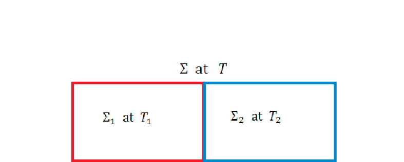
(a) We consider as a simple NEQ example a composite isolated system $\Sigma$, see Fig. 2, consisting of two subsystems $\Sigma_{1}$ and $\Sigma_{2}$ of identical volumes and numbers of particles but at different temperatures $T_{1}$ and $T_{2}$ at any time $t<\tau_{\text{eq}}$ before EQ is reached at $t=\tau_{\text{eq}}$ so the subsystems have different time-dependent energies $E_{1}$ and $E_{2}$, respectively. We assume a diathermal wall separating $\Sigma_{1}$ and $\Sigma_{2}$. Treating each subsystem in EQ at each $t$, we write their entropies as $S_{1}(E_{1},V/2,N/2)$ and $S_{2}(E_{2},V/2,N/2)$, which we simply show as $S_{1}(E_{1})$ and $S_{2}(E_{2})$ as we will not let their volumes and particles numbers change. The entropy $S$ of $\Sigma$ is a function of $E_{1}$ and $E_{2}$. Obviously, $\Sigma$ is in a NEQ state at each $t<\tau_{\text{eq}}$. From $E_{1}$ and $E_{2}$, we form two independent combinations

so that we can express the entropy as $S(E,\xi)$ for $\Sigma$ treated as a black box $\Sigma_{\text{B}}$; we do not need to know about its interior (its inhomogeneity) anymore. Here, $\xi$ plays the role of an internal variable, which continues to relax towards zero as $\Sigma$ approaches EQ. For given $E$ and $\xi$, $S(E,\xi)$ has the maximum possible values since both $S_{1}$ and $S_{2}$ have their maximum value. As we will see below, this is the idea behind the concept of internal equilibrium in which $S(E,\xi)$ is a state function of state variables and continues to increase as $\xi$ decreases and vanishes in EQ. In this state, $S(E,\xi=0)$ has the maximum possible value for fixed $E$ so it becomes a state function. This case and its various extensions are investigated in MNEQT in Sect. VII.1.

(b) We can easily extend the model to include four identical subsystems of fixed and identical volumes and numbers of particles, but of different energies $E_{1},E_{2},E_{3}$, and $E_{4}$. Instead of using these $4$ independent variables, we can use the following four independent combinations

to express the entropy of $\Sigma$ as $S(E,\xi,\xi^{\prime},\xi^{\prime\prime})$. The pattern of extension for this simple case of energy inhomogeneity. is evident.

(c) We make the model a bit more interesting by allowing the volumes $V_{1}$ and $V_{2}$ to also vary as $\Sigma$ equilibrates. Apart from the internal variable $\xi$, we require another internal variable $\xi^{\prime}$ to form two independent combinations

so that we can use $S(E,V,\xi,\xi^{\prime})\doteq S_{1\text{eq}}(E_{1},V_{1})+S_{2\text{eq}}(E_{2},V_{2})$ for the entropy of $\Sigma$ in terms of the entropies of $\Sigma_{1}$ and $\Sigma_{2}$.

(d) In the above examples, we have assumed the subsystems to be in EQ. We now consider when the subsystems are in IEQ. We consider the simple case of two subsystems $\Sigma_{1}$ and $\Sigma_{2}$ of identical volumes and numbers of particles. Each subsystem is in different IEQ states described by $E_{1},\xi_{1}$ and $E_{2},\xi_{2}$. We now construct four independent combinations

which can be used to express the entropy of $\Sigma$ as $S(E,\xi,\xi^{\prime},\xi^{\prime\prime})$.

(e) The example in (a) can be easily extended to the case of expansion and contraction by replacing $E,E_{1}$, and $E_{2}$ by $N,N_{\text{L}}$, and $N_{\text{R}}$ to describe the diffusion of particles from the left (L) region to the right (R) region containing $N_{\text{L}}$ and $N_{\text{R}}$ particles, respectively. The role of $\beta$ and $E$, etc. are played by $\beta\mu$ and $N$, etc.

It should be clear from the above examples that the choice of the number $n^{\ast}$ of internal variables is determined uniquely by a particular modeling of $\Sigma_{\text{b}}$. The number is fixed by matching the number of independent variables needed for the subsystems to be exactly the number of variables needed for $\Sigma_{\text{b}}$. This uniqueness ensures that the entropy of $\Sigma_{\text{b}}$ is uniquely determined by the sum of the entropies of the subsystems. Ensuring subsystems to be in EQ so that their entropies are known, the uniqueness implies that the entropy of $\Sigma_{\text{b}}$ is also known as a function of all the variables of subsystems.

The consideration of dynamics resulting in the simple connectivity of the sample (or phase) space has played a pivotal role in developing the kinetic theory of gases Boltzmann0; Lebowitz, where the interest is at high temperatures Landau; Gujrati-Residual; Gujrati-Symmetry; Gujrati-Poincare. As dynamics is very fast here, it is well known that the ensemble entropy agrees with its temporal formulation. However, at low temperatures, where dynamics becomes sluggish as in a glass Gujrati-book; Palmer; Gutzow; Nemilov, the body can be confined into disjoint components.

Sample (or phase) space confinement at a phase transition such as a liquid-gas transition is well known in equilibrium statistical mechanics Landau; Gujrati-Residual; Gujrati-Symmetry. It also occurs when the body undergoes symmetry breaking such as during magnetic transitions, crystallizations, etc. But confinement can also occur under nonequilibrium conditions, when the observational time scale $\tau_{\text{obs}}$ becomes shorter than the equilibration time $\tau_{\text{eq}}$ Gujrati-book; Palmer; Gutzow; Nemilov, such as for glasses, whose behavior and properties have been extensively studied. In the following, we will focus on $\Sigma_{\text{b}}$.

The issue has been recently considered by us Gujrati-Symmetry, where only energy as an observable was considered. The discussion is easily extended to the present case when confinement occurs for whatever reasons into one of the thermodynamically significant number of disjoint components $\Gamma_{\lambda},\lambda=1,2,3\cdots,\mathcal{C}$, each component corresponding to the same set $\overline{\mathbf{Z}}$. Such a situation arises, for example, in Ising magnets at the ferromagnetic transition., where the system is either confined to $\Gamma_{+}$ with positive magnetization or $\Gamma_{-}$ with negative magnetization. Even a weak external magnetic field $\left|H\right|\rightarrow 0$, that we can control as an observer, will allow the system to make a choice between the two parts of $\Gamma$. It just happens that in this case $\mathcal{C}=2$ and is thermodynamically insignificant.

The situation with glasses or other amorphous materials is very different Palmer, In the first place, $\Gamma$ is a union of thermodynamically significant number $\mathcal{C}\sim e^{cN},c>0,$ disjoint components. In the second place, there is no analog of a symmetry breaking field. Therefore, there is no way to prepare a sample in a given component $\Gamma_{\lambda}$. Thus, the samples will be found in all different components. Taking into consideration disjointness of the components generalizes the number of configurations in Eq. (31) to

where $\mathcal{N}_{k_{\lambda}}$ denotes the number of sample in the microstate $\mathfrak{m}_{k_{\lambda}}$ in the $\lambda$-th component. In terms of $p_{k_{\lambda}}=\mathcal{N}_{k_{\lambda}}(t)/\mathcal{N}$, this combination immediately leads to

References

- (1) R. Clausius, The Mechanical Theory of Heat, Macmillan & Co., London (1879).
- (2) L. Boltzman, Wien Ber. 76, 373 (1877).
- (3) J.W. Gibbs, Elementary Principles in Statistical Mechanics, Yale University Press, CT (1902).
- (4) Th. De Donder and P.V. Rysselberghe, Thermodynamic Theory of Affinity: A Book of Principles. Oxford, England: Oxford University Press (1936).
- (5) E. Fermi, Thermodynamics, Dover, New York (1956).
- (6) R.C. Tolman, The Principles of Statistical Mechanics,Oxford University, London (1959).
- (7) S.A. Rice and P. Gray, The Statistical Mechanics of Simple Liquids, Interscience Publishers, New York (1965).
- (8) F. Reif, Fundamentals of Statistical and Thermal Physics, McGraw-Hill, Inc. New York (1965).
- (9) I. Prigogine, Thermodynamics of Irreversible Processes, Wiley-Interscience, New York (1971).
- (10) L.C. Woods, The Thermodynamics of Fluids Systems, Oxford University Press, Oxford (1975).
- (11) J. Kestin, A course in Thermodynamics, vols. 1 & 2, McGraw-Hill Book Company, New York (1979).
- (12) S.R. de Groot and P. Mazur, Nonequilibrium Thermodynamics, First Edition, Dover, New York (1984).
- (13) H.B. Callen, Thermodynamics and an Introduction to Thermostatistics (2nd ed.), John Wiley & Sons, New York (1985).
- (14) J.R. Waldram, The Theory of Thermodynamics, Cambridge University, Cambridge (1985).
- (15) L.D. Landau, E.M. Lifshitz, Statistical Physics, Vol. 1, Third Edition, Pergamon Press, Oxford (1986).
- (16) R. Balian, From Microphysics to Macrophysics, Vol. 1, Springer-Verlag, Berlin (1991).
- (17) B.G. Eu, Kinetic Theory and Irreversible Thermodynamics, John Wiley, New York (1992).
- (18) D. Kondepudi and I. Prigogine, Modern Thermodynamics, John Wiley and Sons, West Sussex (1998).
- (19) G.D.C. Kuiken, Thermodynamics of Irreversible Processes, John Wiley, Chichester, (1994).
- (20) H.C. Ottinger, Beyond Equilibrium Thermodynamics, Wiley, Hoboken (2005).
- (21) S. Kjelstrum and D. Bedeaux, Nonequilibrium Thermodynamics of Heterogeneous Systems, World-Scientific, Singapore (2008).
- (22) D.J. Evans and G. Morriss, Statistical Mechanics of Nonequilibrium Liquids, Second edition, Cambridge University Press, Cambridge (2008).
- (23) L.D. Landau, E.M. Lifshitz, Quantum Mechanics, Third Edition, Pergamon Press, Oxford (1977).
- (24) J. von Neumann, Mathematical Foundations of Quantum Mechanics, Princeton University Press, N.J. (1996).
- (25) M.H. Partovi, Phys. Rev. Lett. 50,1883 (1983).
- (26) J.D. Beckenstein, Phys. Rev. D 7, 2333 (1973); ibid, 12, 3077 (1975).
- (27) B. Schumacker, Phys. Rev. A 51, 2738 (1995).
- (28) C.H. Bennet, Int. J. Theor. Phys. 21, 905 (1982).
- (29) N. Wiener, Cybernetics, MIT Press, Cambridge (1948).
- (30) C.E. Shannon, Bell Syst. Tech. 27, 379 (1948).
- (31) P.D. Gujrati, arXiv:1304.3768.
- (32) P.D. Gujrati, Entropy, 17, 710 (2015).
- (33) M. Planck, Annale der Physik, 4, 553 (1901).
- (34) L. Boltzmann, Lectures on Gas Theory, University of California Press: Berkeley, CA, USA (1964).
- (35) The number of combinations in Eq. (35) on p. 56 in Boltzmann Boltzmann0 is denoted by , but it is not the number of microstates. The two become the same only when is maximized as discussed on p. 58.
- (36) E.T. Jaynes, Am. J. Phys. 33, 391 (1965).
- (37) P.D. Gujrati, Symmetry 2, 1201 (2010).
- (38) R.C. Bishop, Studies in History and Philosophy of Modern Physics. 35, 1 (2004).
- (39) D.A. Lavis, Philosophy of Science, 75, 682 (2008).
- (40) D. Ruelle, J. Stat. Phys. 85, 1 (1996).
- (41) J. Lebowitz, Rev. Mod. Phys. 71, S346 (1999); S. Goldstein and J.L. Lebowitz, arXiv:cond-mat/0304252v2.
- (42) P.D. Gujrati, Phys. Rev. E 81, 051130 (2010); P.D. Gujrati, arXiv:0910.0026.
- (43) P.D. Gujrati, Phys. Rev. E 85, 041128 (2012); P.D. Gujrati, arXiv:1101.0438.
- (44) P.D. Gujrati, Phys. Rev. E 85, 041129 (2012); P.D. Gujrati, arXiv:1101.0431.
- (45) G.A. Maugin, The Thermodynamics of Nonlinear Irreversible Behaviors,World Scientific, Singapore (1999).
- (46) PD Gujrati, arXiv:1702.00455v1.
- (47) P.D. Gujrati, Entropy 20, 149 (2018).
- (48) P.D. Gujrati, Phys. Rev. E 102, 012140 (2020).
- (49) S.F. Edwards and R.S.B. Oakeshott, Physica 157A, 1080 (1989).
- (50) E. Bouchbinder and J.S. Langer, Phys. Rev. E 80, 031131 (2009); ibid. 031132 (2009); ibid. 031133 (2009).
- (51) I.S. Gutzow and J.W.P. Schmelzer, The Vitreous State: Thermodynamics, Structure, Rheology, and Crystallization, Second Edition, Springer, Berlin (2013).
- (52) S.V. Nemilov, Thermodynamic and Kinetic Aspects of the Vitreous State, CRC Press, Boca Raton (2018).
- (53) P.D. Gujrati, arXiv 0908.1075.
- (54) P.D. Gujrati, arXiv:0803.0983.
- (55) R.J. Palmer, Adv. Phys. 31, 669 (1982).
- (56) P.D. Gujrati in Modeling and Sinulation in Polymers, ed. P.D. Gujrati and A.I. Leonov, Wiley-VCH,Weinheim (2010).
- (57) I. Boyko and P.D. Gujrati, to be published.
- (58) P.D. Gujrati and Tyler Johnson, to be published.
- (59) P.D. Gujrati, arXiv:1512.08744.
- (60) P.D. Gujrati, Phys. Lett. A 384, 126460 (2020).
- (61) F. Wu, L. Chen, S. Wu, F. Sun, and C. Wu, J. Chem. Phys. 124, 214702 (2006).
- (62) C.M. Bender, D.C. Brody and B.K. Meister, J. Phys. A 33, 4427 (2000), and Proc. Roy. Soc. A 461, 733 (2005).
- (63) S.W. Doescher and M.H. Rice, Am. J. Phys. 37, 1246 (1969).
- (64) D.W. Schlitt and C. Stutz, Am. J. Phys. 38, 70 (1970); C. Stutz and D.W. Schlitt, Phys. Rev. A 2, 897 (1970).
- (65) F. Semerianov and P.D. Gujrati, Phys. Rev. E 72, 011102 (2005).
- (66) L. Tonks, Phys. Rev. 50, 955 (1936).
- (67) C. Thompson, Mathematical Statistical Mechanics, Princeton University Press, Princeton, N.J. (1972).
- (68) P.D. Gujrati, J. Chem. Phys. 108, 5104 (1998).
- (69) E.G.D. Cohen, arXiv:1302.2084.
- (70) D. Bawden and L.Robinson, J. Assoc. Inf. Sci. Technol. 66, 1965 (2015).
- (71) E.T. Jaynes, Phys. Rev. 100, 620 (1957).
- (72) P.D. Gujrati, arXiv:1206.0702.