In this paper, we consider only the static and spherically symmetric black holes, whose most general metric takes the form,

$$ds^{2}=-h(r)dt^{2}+{\frac{dr^{2}}{f(r)}}+r^{2}d\Omega^{2}_{2}\,.$$

(1)

We assume that the outer horizon of the black hole is located at $r_{+}$, with $h(r_{+})=f(r_{+})=0$. To study the black hole echoes due to the metric only, we consider the free massless scalar perturbation, whose equation is

$$\Box\psi\equiv{\textstyle{\frac{\scriptstyle 1}{\scriptstyle\sqrt{-g}}}}\partial_{\mu}(\sqrt{-g}g^{\mu\nu}\partial_{\nu}\psi(t,r,\theta,\phi))=0.$$

(2)

For the background metric (1), the equation can be solved straightforwardly using the separation of variables:

$$\psi(t,t,\theta,\phi)=\Sigma_{l.m}{\textstyle{\frac{\scriptstyle\Phi(t,r)}{\scriptstyle r}}}Y_{l,m}(\theta,\phi),$$

(3)

where $Y_{l,m}$ is the spherical harmonics. Under this, the scalar equation (2) reduces to

$$-\frac{\partial^{2}\Phi(t,r)}{\partial t^{2}}+{hf}\frac{\partial^{2}\Phi(t,r)}{\partial r^{2}}+{\textstyle{\frac{\scriptstyle 1}{\scriptstyle 2}}}(fh^{\prime}+hf^{\prime})\frac{\partial\Phi(t,r)}{\partial r}-\bigg({\textstyle{\frac{\scriptstyle l(l+1)}{\scriptstyle r^{2}}}}h+{\textstyle{\frac{\scriptstyle 1}{\scriptstyle 2r}}}(hf)^{\prime}\bigg)\Phi(t,r)=0,$$

(4)

where a prime denotes a derivative with respect to $r$. The radial coordinate $r$ lies in the region $(r_{+},+\infty)$. For QNMs, ingoing and outgoing boundary conditions should be respectively imposed on the horizon $r_{+}$ and at the asymptotically infinity. Therefore QNMs do not probe the spacetime geometry inside the event horizon. It is instructive to use the tortoise coordinate to map the the radial region to $(-\infty,\infty)$. Specifically, we define the tortoise radial coordinate $r_{*}$ by

$$dr_{*}={\frac{dr}{\sqrt{hf}}}\,.$$

(5)

The equation (4) can be cast as

$$-{\frac{\partial^{2}\Phi}{\partial t^{2}}}+{\frac{\partial^{2}\Phi}{\partial r^{2}_{*}}}-V(r)\Phi=0,$$

(6)

where the effective potential $V$ is given by

$$V(r)={\frac{l(l+1)}{r^{2}}}h+{\frac{1}{2r}}(hf)^{\prime}.$$

(7)

It is clear that after imposing the boundary condition, the property of the function $\Phi$ is solely determined by the effective potential $V$. It is worth noting that the tortoise coordinate transformation can stretch the potential but it does not change its shape, characterized by the number of extrema.

It can be easily seen that we have $V(r_{+})=0$ and $V^{\prime}(r_{+})>0$. Furthermore at asymptotically infinity, we have $V(\infty)\rightarrow 0^{+}$ and $V^{\prime}(\infty)\rightarrow 0^{-}$, assuming that $h\sim f\sim 1-2M/r+\cdots$, where $M$ is the mass of the black hole. It follows that the potential $V(r)$ must have at least one maximum. In principle there can exist multiple peaks, with an odd number of total extrema. Typical black holes, including the Schwarzschild and the Reissner-Nordstrøm (RN) black holes, $V(r)$ has one extremum, which is the maximum, in which case, we do not expect to have any echoes, since there is no mechanism for resonance. In order to have echoes, we must have at least three extrema, with a minimum sandwiched between the two maxima. Such configurations of the effective potential arise naturally for wormholes, but are hard to come by in the case of black holes. It is thus natural to explore the conditions for which the potential (7) has at least double peaks.

One clue is provided by the observation that for large $l$, the leading term of the effective potential is dominant, i.e. $V\sim h/r^{2}$, which is precisely the effective potential for determining the photon spheres. The extrema of $h/r^{2}$ with positive $h$ gives the radii of the photon spheres, in the static and spherically symmetric spacetimes. The existence of multiple peaks of our effective potential is then closely related to the existence of multiple photon spheres. Classical black holes with multiple photon spheres are rare, but they do exist and we shall discuss this in section 3.

In this paper, we would like to solve wave equation (6) with the effective potential (7) and obtain the time domain profile of $\Phi(r,t)$. We adopt the the finite difference method, which is effective dealing with the QNMs of both black holes[34] and wormholes [19].

To obtain the finite difference equation, we discretize the coordinates $t=i\Delta t$ and $r_{*}=j\Delta r_{*}$, where the $i$ and $j$ are integers. The scalar field $\Phi$ and the effective potential $V$ are also discretized:

$$\Phi(t,r)=\Phi_{i,j}\equiv(i\Delta t,j\Delta r_{*})\,,\qquad V(r_{*})=V_{j}\equiv V(j\Delta r_{*})\,.$$

(8)

With this, the differential equation (6) becomes a set of iterative algebraic equations:

	$\displaystyle-\frac{\Phi(i+1,j)-2\Phi(i,j)+\Phi(i-1,j)}{\Delta t^{2}}+\frac{\Phi(i,j+1)-2\Phi(i,j)+\Phi(i,j-1)}{\Delta r_{*}^{2}}$		(9)
	$\displaystyle\qquad\qquad-V(j)\Phi(i,j)=0\,.$

Our goal is to solve the above equations, starting from a certain initial wave packet. For convenience, we set it in Gaussian distribution, i.e.

$$\psi(t=0,r_{*})=e^{-\frac{(r_{*}-\bar{a})^{2}}{2}}\,,\qquad\hbox{and}\qquad\psi(t<0,r_{*})=0\,.$$

(10)

The parameter $\bar{a}$ is the location of the center of the initial wave packet. Two inequivalent situations can be considered. One is that the wave packet is outside the double peaks. In this case we find the echoing QNMs have the same characteristics whether it is put close to the horizon or out away from the peaks. We therefore present the results only for the latter case. Another intriguing situation is when we put the initial wave packet in the potential well between the two peaks. We find when the releasing location $\bar{a}$ is closer to the bottom of the potential well, the echo signals will become more distinguishable. Furthermore, the echo frequency, or the number of echoes, roughly doubles the one associated with the wave packet put outside the peaks.

The boundary conditions and (9) are now given by

	$\displaystyle\Phi(t,r_{*})|_{r_{*}\to-\infty}=e^{-{\rm i}{\omega r_{*}}},\qquad\Phi(t,r_{*})|_{r_{*}\to+\infty}=e^{{\rm i}{\omega r_{*}}},$
	$\displaystyle\Phi(i+1,j)=-\Phi(i-1,j)$
	$\displaystyle+\bigg(2-2\frac{\Delta t^{2}}{\Delta r_{*}^{2}}-\Delta t^{2}V(j)\bigg)\Phi(i,j)+\frac{\Delta t^{2}}{\Delta r_{*}^{2}}\bigg(\Phi(i,j+1)+\Phi(i,j-1)\bigg),$		(11)

where $\omega$ is the frequency of the QNMs. (We should distinguish the frequency of the QNMs from the echo frequency.) In fact, it is a free parameter in our numerical calculations. The reason is that the signal has not reached the bound of the grids. According to the von Neumann stability condition, we set $\Delta t/\Delta r_{*}=0.5$ in our numerical calculations. More details are referred to ref. [34].

In this section, we review Einstein-Maxwell gravity extended with a quartic-order quasi-topological term constructed from the Maxwell field strength $F=dA$. The Lagrangian is [31]

$${\cal L}=\sqrt{-g}\Big(R-F^{\mu\nu}F_{\mu\nu}-\alpha\,\big((F^{\mu\nu}F_{\mu\nu})^{2}-2F^{\mu}_{\nu}F^{\nu}_{\rho}F^{\rho}_{\sigma}F^{\sigma}_{\mu}\big)\Big)\,,$$

(12)

where $\alpha$ is the coupling constant of the quasi-topological term. The theory admits an exact solution of asymptotically-flat dyonic black holes that are both static and spherically symmetric:

$$ds^{2}=-hdt^{2}+{\frac{dr^{2}}{h}}+r^{2}\big(d\theta^{2}+\sin^{2}\theta\,d\varphi^{2}\big)\,,\quad F=-{\frac{qr^{2}}{r^{4}+4\alpha p^{2}}}dt\wedge dr+p\sin\theta d\theta\wedge d\varphi\,,$$

(13)

with

$$h=1-\frac{2M}{r}+\frac{p^{2}}{r^{2}}+\frac{q^{2}}{r^{2}}\,_{2}F_{1}\Big(\frac{1}{4},1;\frac{5}{4};-\frac{4\alpha\,p^{2}}{r^{4}}\Big)\,.$$

(14)

The general solution contains three integration constants, the mass $M$, electric and magnetic charges $(q,p)$. When $\alpha qp=0$, the solution reduces to the usual RN black hole. The property of these black holes were analysed in [31]. They all satisfy DEC, but can violate SEC. For suitable parameters, black holes with four horizon can emerge. In this paper, we are interested in black holes with two horizons, but with an unusual feature that the profile function $h$ is not monotonous outside the horizon. It has an extra wiggle such that the gravity force can vanish and even be repulsive in certain finite region outside the horizon. This feature is a direct consequence of the SEC violation.

For a concrete example, we choose the parameters, e.g. $(\alpha,p,q)=(149.90,0.945,6.863)$. For $M<6.370$, solution is over charged and the curvature singularity at $r=0$ is naked. When $6.355<M<6.729$, the black hole has two horizons and $h$ is not monotonous outside the outer horizon, but has a wiggle with a local maximum and a minimum. Further increasing the mass such that $6.723<M<6.760$, the local minimum dips down to be negative so that the black hole has four horizons. When $M>6.760$, the two inner horizons disappear and the black hole reverts back to have two horizons. In the last two cases, the function $h$ is monotonous outside the outer horizon. In Fig. 1, we present the plots for the function $h$ for $M=6.80$ and $M=6.65$.

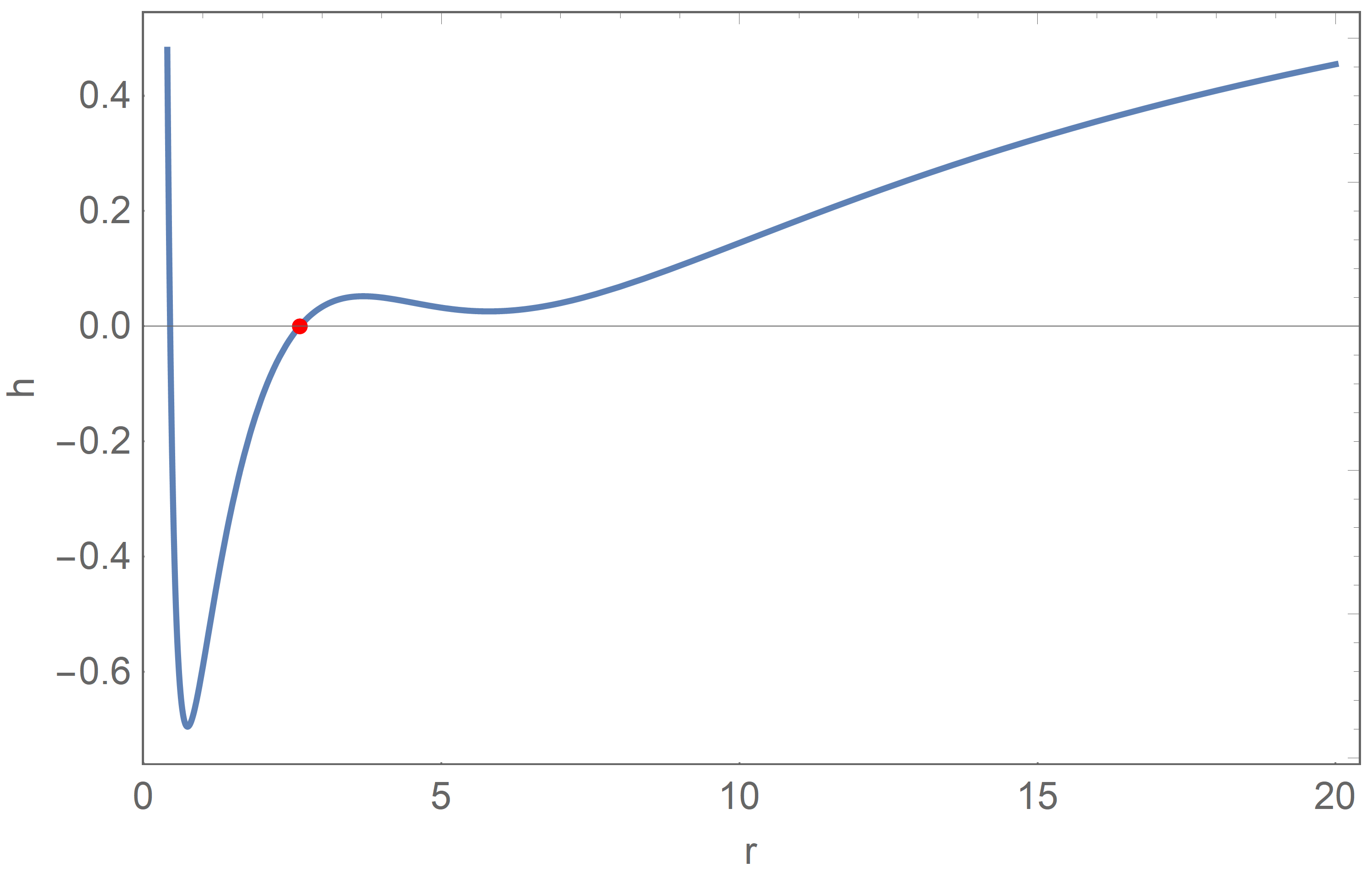
We see from Fig. 1 that both black holes with $M=6.80$ and $M=6.65$ have two horizons. However, when $M=6.80$, the function $h$ is monotonous outside the horizon, but it has a wiggle when $M=6.65$. This extra wiggle implies that the black hole has three photo spheres, with a stable photon sphere sandwiched between two unstable ones [31]. As we have discussed earlier, we expect that such spacetime geometry will give rise the effective potential with double peaks, which we discuss in the next subsection.

The effective potential of the massless scalar wave is given (7). For our case, we have $f=h$, with h given by (14). We find that there are two types of the effective potentials, depending on the values of the black hole parameters. One involves a single peak, and the other has double peaks. Taking the same values associated with Fig. 1, we present the corresponding effective potentials using the tortoise coordinates in Fig. 2.

As we see from Fig. 2 that when $M=6.80$, the effective potential has a single peak, which is typical for many black holes including the Schwarzschild and RN black holes. It has been pointed out in ref.[30] that such black holes can not produce echoes, without introducing a reflective boundary condition by hand.

To produce echoes in classical black holes, it calls for effective potentials with at least two peaks. It is easy to be realized in wormhole metrics [17, 18, 19, 20]. However, there are few such black holes. For the $M=6.65$ black hole, the double-peak potential is achieved by violating SEC such that gravity can be repulsive in certain regions of spacetime. However, since our solutions satisfy DEC, they can nevertheless be models for realistic black holes.

Having established that the double-peak potential can arise, we explore the parameter space around the above example to see how the potential depends on various parameters including the mass, charge and also the $l$ parameter associated with the spherical harmonics. In order not to interrupt the flow of the main text, we present all the plots of the double-peak potentials in appendix A. The effective potential depends on $(M,q,p,l,\alpha)$. In Fig. 5, Fig. 7 and Fig. 9, we give the effective potentials with varying $M$, $q$ and $\ell$ respectively. It should be mentioned that when $l\neq 0$, the effective potential is always nonnegative. However, when $\ell=0$, there may exist regions where the potential becomes negative. We find that in this case the echoes are not discernible. In the next subsection, we study the time-domain profiles of the corresponding QNMs and see that they generally produce echoes.

While the existence of multiple-photon spheres provides the inspiration for double-peak potentials when the first term in (7) is dominant, the second term in (7) suggests that echoes may happen even when the function $h$ is monotonous, provided that $h^{\prime}$ is not. We shall present such an example in the next section, together with its echoing QNM.

Here we present the results for the first case. For the purpose of comparison, we first give the QNM when the potential has only one peak. We consider the $M=6.80$ case of Figs. 1, 2. As expected, the original wave packet evolves as a damping oscillator, and it produces no echoes, as can be seen by the left column of Fig. 3.

For the double-peak potentials, we can observe the echo signals after the initial damping of the wave packet. A concrete example of the time-domain profile of the echoes is presented in right column of Fig. 3. It is clear that the echoes arise because of resonant reflection by the two peaks. Therefore the frequency, or the number of echoes does not depend on the releasing position, as long as they are outside the two peaks. (We shall study presently the case when the initial wave packet is released inside the two peaks.)

As we discussed in the previous section, we have obtained many examples of double-peak potentials, by varying parameters such as $M$, $q$ and $l$. We construct the corresponding QNMs and obtain the time-domain profiles. We present the results in the appendix A in Fig. 6, Fig. 8 and Fig. 10 respectively. As we can see, the signature of echo signals depends on many factors and to distinguish them requires precision measurements. One special case is worth mentioning, namely $l=0$. The effective potential can be negative in some regions and the echo signals are hardly discernible. This phenomenon was first noted in the wormhole cases [36].

From these examples, one might draw a conclusion that the double-peaks potential arises only in the case when $h(r)$ is not monotonically increasing. However, this is not true. We find an example where $h(r)$ is in fact monotonically increasing outside the horizon, but the corresponding effective potential continue to have double peaks. This case arise when we choose the following parameters:

$$\alpha=123.90\,,\quad p=1.181\,,\quad q=6.863\,,\quad l=3\,,\quad M=6.58\,.$$

(15)

It is clear that the second term in (7) can also give nontrivial contribution since $h^{\prime}$ is not monotonous is this case. Our numerical study shows that this black hole can also produce echoes, although the signals are less clear in later time. We show the results of this example in Fig. 11 in the appendix.

In the previous subsection, we focus on echoes of the initial wave packet released outside the two peaks of the effective potential. We now release it in the potential well between the two peaks. As a concrete example, we consider the potential given in Fig. 5, with $\alpha=149.90,p=0.945,q=6.863,l=1,M=6.7$. We find that the echo signals become more sensitive to the exact release location. In particular the echoes become more distinguished when the releasing location is at the bottom of the potential well, in which case, we find that the echo frequency nearly doubles. This phenomenon is explicitly depicted in Fig. 4, and we see that echoes of the wave packet outside the peak is much more pronounced.

References

- [1] V. Cardoso, E. Franzin and P. Pani, “Is the gravitational-wave ringdown a probe of the event horizon?,” Phys. Rev. Lett. 116, no.17, 171101 (2016) [erratum: Phys. Rev. Lett. 117, no.8, 089902 (2016)] doi:10.1103/PhysRevLett.116.171101 [arXiv:1602.07309 [gr-qc]].
- [2] E. Berti, V. Cardoso and A.O. Starinets, “Quasinormal modes of black holes and black branes,” Class. Quant. Grav. 26, 163001 (2009) doi:10.1088/0264-9381/26/16/163001 [arXiv:0905.2975 [gr-qc]].
- [3] Z. Mark, A. Zimmerman, S.M. Du and Y. Chen, “A recipe for echoes from exotic compact objects,” Phys. Rev. D 96, no.8, 084002 (2017) doi:10.1103/PhysRevD.96.084002 [arXiv:1706.06155 [gr-qc]].
- [4] H. Huang and J. Yang, “Charged Ellis wormhole and black bounce,” Phys. Rev. D 100, no.12, 124063 (2019) doi:10.1103/PhysRevD.100.124063 [arXiv:1909.04603 [gr-qc]].
- [5] H. Huang, H. Lü and J. Yang, “Bronnikov-like wormholes in Einstein-scalar gravity,” [arXiv:2010.00197 [gr-qc]].
- [6] P. Kanti, B. Kleihaus and J. Kunz, “Wormholes in dilatonic Einstein-Gauss-Bonnet theory,” Phys. Rev. Lett. 107, 271101 (2011) doi:10.1103/PhysRevLett.107.271101 [arXiv:1108.3003 [gr-qc]].
- [7] B. Kleihaus and J. Kunz, “Rotating Ellis wormholes in four dimensions,” Phys. Rev. D 90, 121503 (2014) doi:10.1103/PhysRevD.90.121503 [arXiv:1409.1503 [gr-qc]].
- [8] F.E. Schunck and E.W. Mielke, “General relativistic boson stars,” Class. Quant. Grav. 20, R301-R356 (2003) doi:10.1088/0264-9381/20/20/201 [arXiv:0801.0307 [astro-ph]].
- [9] B. Kleihaus, J. Kunz and M. List, “Rotating boson stars and Q-balls,” Phys. Rev. D 72, 064002 (2005) doi:10.1103/PhysRevD.72.064002 [arXiv:gr-qc/0505143 [gr-qc]].
- [10] B. Hartmann, B. Kleihaus, J. Kunz and M. List, “Rotating boson stars in 5 dimensions,” Phys. Rev. D 82, 084022 (2010) doi:10.1103/PhysRevD.82.084022 [arXiv:1008.3137 [gr-qc]].
- [11] A. Almheiri, D. Marolf, J. Polchinski and J. Sully, “Black Holes: Complementarity or Firewalls?,” JHEP 02, 062 (2013) doi:10.1007/JHEP02(2013)062 [arXiv:1207.3123 [hep-th]].
- [12] D.E. Kaplan and S. Rajendran, “Firewalls in general relativity,” Phys. Rev. D 99, no.4, 044033 (2019) doi:10.1103/PhysRevD.99.044033 [arXiv:1812.00536 [hep-th]].
- [13] J. Abedi, H. Dykaar and N. Afshordi, “Echoes from the abyss: tentative evidence for Planck-scale structure at black hole horizons,” Phys. Rev. D 96, no.8, 082004 (2017) doi:10.1103/PhysRevD.96.082004 [arXiv:1612.00266 [gr-qc]].
- [14] J. Abedi, H. Dykaar and N. Afshordi, “Echoes from the abyss: the holiday edition!,” [arXiv:1701.03485 [gr-qc]].
- [15] V. Cardoso and P. Pani, “Tests for the existence of black holes through gravitational wave echoes,” Nature Astron. 1, no.9, 586-591 (2017) doi:10.1038/s41550-017-0225-y [arXiv:1709.01525 [gr-qc]].
- [16] V. Cardoso, S. Hopper, C.F.B. Macedo, C. Palenzuela and P. Pani, “Gravitational-wave signatures of exotic compact objects and of quantum corrections at the horizon scale,” Phys. Rev. D 94, no.8, 084031 (2016) doi:10.1103/PhysRevD.94.084031 [arXiv:1608.08637 [gr-qc]].
- [17] P. Bueno, P.A. Cano, F. Goelen, T. Hertog and B. Vercnocke, “Echoes of Kerr-like wormholes,” Phys. Rev. D 97, no.2, 024040 (2018) doi:10.1103/PhysRevD.97.024040 [arXiv:1711.00391 [gr-qc]].
- [18] K.A. Bronnikov and R.A. Konoplya, “Echoes in brane worlds: ringing at a black hole–wormhole transition,” Phys. Rev. D 101, no.6, 064004 (2020) doi:10.1103/Phys RevD.101.064004 [arXiv:1912.05315 [gr-qc]].
- [19] H. Liu, P. Liu, Y. Liu, B. Wang and J.P. Wu, “Echoes from phantom wormholes,” Phys. Rev. D 103, no.2, 024006 (2021) doi:10.1103/PhysRevD.103.024006 [arXiv:2007.09078 [gr-qc]].
- [20] M.Y. Ou, M.Y. Lai and H. Huang, “Echoes from asymmetric wormholes and black bounce,” [arXiv:2111.13890 [gr-qc]].
- [21] R.A. Konoplya, Z. Stuchlík and A. Zhidenko, “Echoes of compact objects: new physics near the surface and matter at a distance,” Phys. Rev. D 99, no.2, 024007 (2019) doi:10.1103/PhysRevD.99.024007 [arXiv:1810.01295 [gr-qc]].
- [22] D. Kartini and A. Sulaksono, “Gravitational wave echoes from quark stars,” J. Phys. Conf. Ser. 1572, 012034 (2020) doi:10.1088/1742-6596/1572/1/012034
- [23] R. Dey, S. Chakraborty and N. Afshordi, “Echoes from braneworld black holes,” Phys. Rev. D 101, no.10, 104014 (2020) doi:10.1103/PhysRevD.101.104014 [arXiv: 2001.01301 [gr-qc]].
- [24] A. Chowdhury and N. Banerjee, “Echoes from a singularity,” Phys. Rev. D 102, no.12, 124051 (2020) doi:10.1103/PhysRevD.102.124051 [arXiv:2006.16522 [gr-qc]].
- [25] Q. Wang, N. Oshita and N. Afshordi, “Echoes from quantum black holes,” Phys. Rev. D 101, no.2, 024031 (2020) doi:10.1103/PhysRevD.101.024031 [arXiv:1905.00446 [gr-qc]].
- [26] K. Saraswat and N. Afshordi, “Quantum nature of black holes: fast scrambling versus echoes,” JHEP 04, 136 (2020) doi:10.1007/JHEP04(2020)136 [arXiv:1906.02653 [hep-th]].
- [27] N. Oshita, D. Tsuna and N. Afshordi, “Quantum black hole seismology I: echoes, ergospheres, and spectra,” Phys. Rev. D 102, no.2, 024045 (2020) doi:10.1103/Phys RevD.102.024045 [arXiv:2001.11642 [gr-qc]].
- [28] S.K. Manikandan and K. Rajeev, “On a new kind of echo from quantum black holes,” [arXiv:2112.08773 [gr-qc]].
- [29] H. Liu, W.L. Qian, Y. Liu, J.P. Wu, B. Wang and R.H. Yue, “Alternative mechanism for black hole echoes,” Phys. Rev. D 104, no.4, 044012 (2021) doi:10.1103/PhysRev D.104.044012 [arXiv:2104.11912 [gr-qc]].
- [30] G. D’Amico and N. Kaloper, “Black hole echoes,” Phys. Rev. D 102, no.4, 044001 (2020) doi:10.1103/PhysRevD.102.044001 [arXiv:1912.05584 [gr-qc]].
- [31] H.S. Liu, Z.F. Mai, Y.Z. Li and H. Lü, “Quasi-topological electromagnetism: dark energy, dyonic Black Holes, stable photon spheres and hidden electromagnetic duality,” Sci. China Phys. Mech. Astron. 63, 240411 (2020) doi:10.1007/s11433-019-1446-1 [arXiv:1907.10876 [hep-th]].
- [32] A. Cisterna, G. Giribet, J. Oliva and K. Pallikaris, “Quasitopological electromagnetism and black holes,” Phys. Rev. D 101, no.12, 124041 (2020) doi:10.1103/Phys RevD.101.124041 [arXiv:2004.05474 [hep-th]].
- [33] R. Dey, S. Biswas and S. Chakraborty, “Ergoregion instability and echoes for brane world black holes: scalar, electromagnetic, and gravitational perturbations,” Phys. Rev. D 103, no.8, 084019 (2021) doi:10.1103/PhysRevD.103.084019 [arXiv:2010.07966 [gr-qc]].
- [34] Z. Zhu, S.J. Zhang, C.E. Pellicer, B. Wang and E. Abdalla, “Stability of Reissner-Nordström black hole in de Sitter background under charged scalar perturbation,” Phys. Rev. D 90, no.4, 044042 (2014) doi:10.1103/PhysRevD.90.044042 [arXiv: 1405.4931 [hep-th]].
- [35] R.A. Konoplya and A. Zhidenko, “Quasinormal modes of black holes: from astrophysics to string theory,” Rev. Mod. Phys. 83, 793-836 (2011) doi:10.1103/RevModPhys.83.793 [arXiv:1102.4014 [gr-qc]].
- [36] M.S. Churilova and Z. Stuchlik, “Ringing of the regular black-hole/wormhole transition,” Class. Quant. Grav. 37, no.7, 075014 (2020) doi:10.1088/1361-6382/ab7717 [arXiv:1911.11823 [gr-qc]].