跳到论文正文
W Papers独立论文阅读器 arXiv:2112.14726 论文正文 计算阅读时间 · 0%
引用这篇论文根据当前论文元数据生成,正式投稿前建议核对。


License: arXiv.org perpetual non-exclusive license
arXiv:2112.14726v2 [cs.IT] 29 May 2022

Uniqueness Theorems for Tomographic Phase Retrieval with Few Coded Diffraction Patterns

Albert Fannjiang Address: Department of Mathematics, University of California, Davis, California 95616, USA. Email: fannjiang@math.ucdavis.edu
Abstract.

3D tomographic phase retrieval under the Born approximation for discrete objects supported on a n×n×nn\times n\times n grid is analyzed. It is proved that nn projections are sufficient and necessary for unique determination by computed tomography (CT) with full projected field measurements and that n+1n+1 coded projected diffraction patterns are sufficient for unique determination, up to a global phase factor, in tomographic phase retrieval. Hence n+1n+1 is nearly, if not exactly, the minimum number of diffractions patterns needed for 3D tomographic phase retrieval under the Born approximation.

1. Introduction

Tomography is a commonly used method in a wide range of applications such as computed tomography [21], 3D diffractive imaging [7] and quantum state measurement [17].

Mathematically speaking, the forward model of tomography is based on various approximations of the nonlinear inverse scattering formulation (for example, the Lippmann-Schwinger integral equation). A simplification common to all current tomographic methods (except for geophysical applications) is based on either the Born or the Rytov approximation. The latter reduces to computed tomography (CT) in the limit of geometrical optics. The inversion methods of CT, which ignores the diffraction and scattering effects, have been well studied and documented [21]. On the other hand, the phase-unwrapping problem inherent to the Rytov approximation (see Section 2) is a largely unsolved problem and a major road block to its implementation [7].

An additional complication occurs in X-ray, optical scattering [2], electron diffraction [12, 11] as well as quantum state tomography [17], where only intensity measurements can be performed. This gives rise to the phase problem which requires phase retrieval techniques for solutions [10].

This brief note considers the imaging set-up based on the Born approximation where diffraction patterns (hence intensity-only measurements) in various directions are measured and used to determine the 3D object.

In particular, we address the uniqueness question: Under what measurement schemes and with how many diffraction patterns, can one determine the 3D object uniquely (up to a global phase factor)?

To answer this question in a quantitative way, it is instructive (even imperative) to work with a discrete setting. After introducing the Born-projection approximation in Section 2 and laying out the discrete framework in Section 3, we recall some basic results about diffraction patterns in Section 4, in particular how the use of a random mask can improve the quality of the measurement data (see also Remark 5.3). In Section 5 we first prove that with a random mask in the measurement of diffraction patterns, the tomographic phase retrieval problem reduces to that of CT modulo a simple ambiguity (Theorem 5.1). We then eliminate this ambiguity by deploying a sufficiently diverse set of n+1n+1 projections under the prior constraint that the object does not become part of a line segment in any projection in the measurement scheme. As the uniqueness condition of nn projections required for the standard CT (Theorem 5.5) sets a lower bound on the number of diffraction patterns for tomographic phase retrieval, the uniqueness condition of n+1n+1 diffraction patterns (Theorem 5.8) is nearly optimal. We conclude with several remarks in Section 6.

2. Born and projection approximations
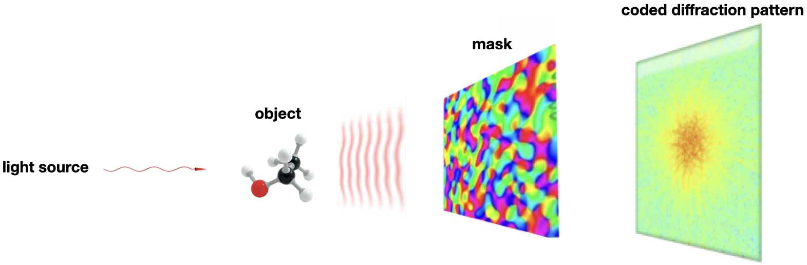
Refer to caption
Figure 1. Diffraction pattern coded by a random mask placed behind the object. Different projections can be implemented by orientating the object in the corresponding direction, with the measurement set-up fixed. See, e.g. [19] for an similar experimental set-up

In scattering theory, the full field u=ui+usu=u_{i}+u_{s} is written as the sum of the incident field uiu_{i} and the scattered field usu_{s}. In the continuum setting, the full field u⁡(𝐫)u(\mathbf{r}) is governed by the Lippmann-Schwinger equation

(1) u⁡(𝐫)=ui​(𝐫)+∫d​𝐫′​G​(𝐫−𝐫′)​f​(𝐫′)​u​(𝐫′)\displaystyle u(\mathbf{r})=u_{i}(\mathbf{r})+\int d\mathbf{r}^{\prime}G(\mathbf{r}-\mathbf{r}^{\prime})f(\mathbf{r}^{\prime})u(\mathbf{r}^{\prime})

where ff is the inhomogeneity, also called scattering potential, and GG is the Green’s function of the free-space Helmholtz equation [7].

Under the weak scatter assumption |us|≪|ui|,|u_{s}|\ll|u_{i}|, uu in the (first-order) Born approximation is given by

(2) u⁡(𝐫)=ui​(𝐫)+∫d​𝐫′​G​(𝐫−𝐫′)​f​(𝐫′)​ui​(𝐫′).\displaystyle u(\mathbf{r})=u_{i}(\mathbf{r})+\int d\mathbf{r}^{\prime}G(\mathbf{r}-\mathbf{r}^{\prime})f(\mathbf{r}^{\prime})u_{i}(\mathbf{r}^{\prime}).

Under the Fresnel approximation (with the zz-axis as the optical axis, say),

(3) G⁡(𝐫)=−14​π​ei​κ​|𝐫||𝐫|≈−14​π​|z|​ei​κ​|z|​ei​κ2​x2+y2|z|\displaystyle G(\mathbf{r})={-1\over 4\pi}{e^{{\rm i}\kappa|\mathbf{r}|}\over|\mathbf{r}|}\approx{-1\over 4\pi|z|}e^{{\rm i}\kappa|z|}e^{{\rm i}{\kappa\over 2}{x^{2}+y^{2}\over|z|}}

and hence (2) becomes

(4) ui​(𝐫)−ei​κ​z4​π​∫d​x′​d​y′​∫d​z′​f⁡(x′,y′,z′)|z−z′|​ei​κ2​(x−x′)2+(y−y′)2|z−z′|​e−i​κ​z′​ui​(x′,y′,z′).\displaystyle u_{i}(\mathbf{r})-{e^{{\rm i}\kappa z}\over 4\pi}\int dx^{\prime}dy^{\prime}\int dz^{\prime}{f(x^{\prime},y^{\prime},z^{\prime})\over|z-z^{\prime}|}e^{{\rm i}{\kappa\over 2}{(x-x^{\prime})^{2}+(y-y^{\prime})^{2}\over|z-z^{\prime}|}}e^{-{\rm i}\kappa z^{\prime}}u_{i}(x^{\prime},y^{\prime},z^{\prime}).

We think of the scattering process as consisting of two stages: First, the plane wave (ui​(𝐫)=ei​κ​zu_{i}(\mathbf{r})=e^{{\rm i}\kappa z}) illuminates and exits the scattering object; second, the exit wave transmits through a mask (located at z=0z=0) and propagates toward the detector.

In the first stage, consider the high Fresnel number regime

(5) NF=ℓ2λ​z0≫1,\displaystyle N_{F}={\ell^{2}\over\lambda z_{0}}\gg 1,

where ℓ\ell is the typical size to be resolved, λ\lambda the wavelength and z0z_{0} the thickness of the object. In this limit (5),

−i​κ2​π​|z−z′|​ei​κ2​(x−x′)2+(y−y′)2|z−z′|⟶δ⁡(x−x′,y−y′),as​NF→∞{-{\rm i}\kappa\over 2\pi|z-z^{\prime}|}e^{{\rm i}{\kappa\over 2}{(x-x^{\prime})^{2}+(y-y^{\prime})^{2}\over|z-z^{\prime}|}}\longrightarrow\delta(x-x^{\prime},y-y^{\prime}),\quad\mbox{as}\,\,N_{F}\to\infty

for all z≠z′z\neq z^{\prime}, the exit wave (4) at z=0z=0 is approximated by

(6) vB​(x,y)=1−i2​κ​∫d​z′​f​(x,y,z′).\displaystyle v_{B}(x,y)=1-{{\rm i}\over 2\kappa}\int dz^{\prime}{f(x,y,z^{\prime})}.

The right hand side of (6) is the projection approximation under the first-order Born assumption. On the other hand, the exit wave with the Rytov approximation is given by

vR(x,y)=exp[−i2​κ∫dz′f(x,y,z′)].\displaystyle v_{R}(x,y)=\exp\left[-{{\rm i}\over 2\kappa}\int dz^{\prime}{f(x,y,z^{\prime})}\right].

Since

(7) vB−1=ln⁡vRmod​  2​π​i,\displaystyle v_{B}-1=\ln v_{R}\quad\hbox{mod}\,\,2\pi{\rm i},

the Born scattered field is the unwrapped phase of the Rytov approximation.

In short, the Born-projection approximation is the linear approximation of the Rytov-projection approximation and both approximations employ the projection approximation [6].

The projection approximation corresponds to light propagation through the scatterer in parallel straight lines. Its validity, however, depends on the spatial resolution of the imaging system as follows.

Radiation of wavelength λ\lambda scattered by features of size ℓ\ell, that are to be resolved, would have a maximum diffraction angle of the order of Δ​θ=λ/ℓ.\Delta\theta=\lambda/\ell. Hence the maximum spread of the radiation at the exit plane would be Δ​θ​z0\Delta\theta z_{0} where z0z_{0} is the thickness of the sample. The projection approximation is valid if the spread is much smaller than the resolution, i.e.

(8) λ​z0/ℓ≪ℓ.\displaystyle\lambda z_{0}/\ell\ll\ell.

which is exactly equivalent to the high Fresnel number regime (5) [22].

At the second stage, the exit wave vBv_{B} is first multiplied by the mask function μ\mu and then propagates into the far-field as ℱ⁡(μ⋅vB){\mathcal{F}}(\mu\cdot v_{B}) where ℱ{\mathcal{F}} is the Fourier transform in the transverse variables. The measured coded diffraction pattern |ℱ⁡(μ⋅vB)|2|{\mathcal{F}}(\mu\cdot v_{B})|^{2} is given by

(9) |ℱ⁡(μ⋅vB)|2\displaystyle|{\mathcal{F}}(\mu\cdot v_{B})|^{2} =\displaystyle= |ℱ⁡(μ)|2+1κ​ℑ⁡{ℱ​μ¯⋅ℱ⁡(μ​∫f​d​z′)}+14​κ2​|ℱ⁡(μ​∫f​d​z′)|2\displaystyle|{\mathcal{F}}(\mu)|^{2}+{1\over\kappa}\Im\{{\overline{{\mathcal{F}}\mu}\cdot{\mathcal{F}}(\mu\int fdz^{\prime})}\}+{1\over 4\kappa^{2}}|{\mathcal{F}}(\mu\int fdz^{\prime})|^{2}

where ℑ\Im denotes the imaginary part. This technique, with or without coded aperture, is sometimes called the propagation-based phase contrast method [22].

Tomographic microscopy based on the linear forward model ignoring the nonlinear term |ℱ⁡(μ​∫d​z′​f)|2|{\mathcal{F}}(\mu\int dz^{\prime}f)|^{2} on the right hand side of (9) is a form of bright-field imaging (see [18, 23]). As (9) represents the interference pattern between the reference wave ℱ⁡(μ){\mathcal{F}}(\mu) and the masked object wave −iℱ(μ∫fdz′)/(2κ)-{\rm i}{\mathcal{F}}(\mu\int fdz^{\prime})/(2\kappa), reconstruction from the linear term in (9) can be performed by conventional holographic techniques [25, 26].

Adopting the dark-field mode of imaging (see [15] where the pupil or probe function plays the role of coded aperture), we focus on the more challenging nonlinear term as the measurement data and analyze the inherent information content therein. The (nonlinear) combination of the coded aperture and the Fourier transform is a key ingredient of our approach. The next key ingredient to an information-based approach is discretization.

3. Discrete tomography

To motivate the discrete setup, consider the continuum setting. It is a classical result that a compactly supported function on, e.g. the cube, is uniquely determined by  the Fourier transform (magnitude & phase) in any infinite set of projections ([14], Proposition 7.8) while for any finite set of projections, counterexamples to unique determination can be constructed ([14], Proposition 7.9).

As a consequence, uniqueness with Fourier intensity data in the continuum setting would require additional assumptions besides an infinite number of projections. It is not currently known, however, what additional assumptions are needed to guarantee uniqueness with intensity-only measurements.

Working with a discrete set-up we aim to derive a quantitative, information-based theory of uniqueness. To this end, we adopt the framework of [1] whose main advantage is preserving the fundamental Fourier slice theorem (Theorem 3.1).

For simplicity, we choose the physical units so that κ=2​π.\kappa=2\pi. Let ⟦k,l⟧\llbracket k,l\rrbracket denote the integers between and including the integers kk and ll. We define a 3D n×n×nn\times n\times n object as the set

(10) f={f(i,j,k)∈ℂ:i,j,k∈ℤn}\displaystyle f=\{f(i,j,k)\in\mathbb{C}:i,j,k\in\mathbb{Z}_{n}\}

where

ℤn\displaystyle\mathbb{Z}_{n} =\displaystyle= {⟦−n/2,n/2−1⟧if n is an even integer;⟦−(n−1)/2,(n−1)/2⟧if n is an odd integer.\displaystyle\left\{\begin{array}[]{lll}\llbracket-n/2,n/2-1\rrbracket&&\mbox{if $n$ is an even integer;}\\ \llbracket-(n-1)/2,(n-1)/2\rrbracket&&\mbox{if $n$ is an odd integer.}\end{array}\right.

We define three families of line segments, the xx-lines, yy-lines, and zz-lines. Formally, a xx-line, denoted by ℓx⁡(α,β)​(c1,c2)\ell_{x(\alpha,\beta)}(c_{1},c_{2}), is defined as

(14) ℓx⁡(α,β)​(c1,c2):[yz]=[α​x+c1β​x+c2]\displaystyle\ell_{x(\alpha,\beta)}(c_{1},c_{2}):\left[\begin{matrix}y\\ z\end{matrix}\right]=\left[\begin{matrix}\alpha x+c_{1}\\ \beta x+c_{2}\end{matrix}\right] c1,c2∈ℤ2​n−1,x∈ℤn\displaystyle{c_{1},c_{2}\in\mathbb{Z}_{2n-1}},\quad x\in\mathbb{Z}_{n}

To avoid wraparound of xx-lines with |α|,|β|≤1|\alpha|,|\beta|\leq 1, we can zero-pad ff in a larger lattice ℤp3\mathbb{Z}^{3}_{p} with p≥2​n−1.p\geq 2n-1. This is particularly important when it comes to define the X-ray transform by a line sum (cf. (20)-(22)) without wrapping around the object domain.

Similarly, a yy-line and a zz-line are defined as

(15) ℓy⁡(α,β)​(c1,c2):[xz]=[α​y+c1β​y+c2]\displaystyle\ell_{y(\alpha,\beta)}(c_{1},c_{2}):\left[\begin{matrix}x\\ z\end{matrix}\right]=\left[\begin{matrix}\alpha y+c_{1}\\ \beta y+c_{2}\end{matrix}\right] c1,c2∈ℤ2​n−1,y∈ℤn,\displaystyle c_{1},c_{2}\in\mathbb{Z}_{2n-1},\quad y\in\mathbb{Z}_{n},
(16) ℓz⁡(α,β)​(c1,c2):[xy]=[α​z+c1β​z+c2]\displaystyle\ell_{z(\alpha,\beta)}(c_{1},c_{2}):\left[\begin{matrix}x\\ y\end{matrix}\right]=\left[\begin{matrix}\alpha z+c_{1}\\ \beta z+c_{2}\end{matrix}\right] c1,c2∈ℤ2​n−1,z∈ℤn.\displaystyle c_{1},c_{2}\in\mathbb{Z}_{2n-1},\quad z\in\mathbb{Z}_{n}.

We denote the sets of all xx-lines, yy-lines, and zz-lines by ℒx,ℒy,{\mathcal{L}}_{x},{\mathcal{L}}_{y}, and ℒz{\mathcal{L}}_{z}, respectively.

Also, we denote the family of lines that corresponds to a fixed pair (α,β)(\alpha,\beta) and variable intercepts (c1,c2)(c_{1},c_{2}) by ℓx⁡(α,β),ℓy⁡(α,β)\ell_{x(\alpha,\beta)},\ell_{y(\alpha,\beta)} and ℓz⁡(α,β)\ell_{z(\alpha,\beta)} for a family of parallel xx-lines, yy-lines, and zz-lines, respectively. Note that ℓx⁡(1,β)=ℓy⁡(1,β),ℓx⁡(α,1)=ℓz⁡(1,α)\ell_{x(1,\beta)}=\ell_{y(1,\beta)},\ell_{x(\alpha,1)}=\ell_{z(1,\alpha)} and ℓy⁡(α,1)=ℓz⁡(α,1).\ell_{y(\alpha,1)}=\ell_{z(\alpha,1)}.

Let fxf_{x} be the continuous interpolation of ff in the directions perpendicular to xx as follows:

(17) fx​(i,y,z)\displaystyle f_{x}(i,y,z) =\displaystyle= ∑j∈ℤn∑k∈ℤnf⁡(i,j,k)​Dp​(y−j)​Dp​(z−k),y,z∈ℝ\displaystyle\sum_{j\in\mathbb{Z}_{n}}\sum_{k\in\mathbb{Z}_{n}}f(i,j,k)D_{p}(y-j)D_{p}(z-k),\quad y,z\in\mathbb{R}

where DpD_{p} is the pp-periodic Dirichlet kernel given by

Dp​(t)=1p​∑l∈ℤpei2​π​l​t/p\displaystyle D_{p}(t)={1\over p}\sum_{l\in\mathbb{Z}_{p}}e^{{\rm i}2\pi lt/p} =\displaystyle= {1,t=m​p,m∈ℤsin⁡(π​t)p​sin⁡(π​t/p),else.\displaystyle\left\{\begin{matrix}1,&t=mp,\quad m\in\mathbb{Z}\\ {\sin{(\pi t)}\over p\sin{(\pi t/p)}},&\mbox{else}.\end{matrix}\right.

In particular, Dp​(t)=0D_{p}(t)=0 for t∈ℤ/ℤpt\in\mathbb{Z}/\mathbb{Z}_{p}, i.e. [Dp​(i−j)]i,j∈ℤp[D_{p}(i-j)]_{i,j\in\mathbb{Z}_{p}} is the p×pp\times p identity matrix.

Similarly we define the interpolation of ff perpendicular to yy and zz, respectively, as

(18) fy​(x,j,z)\displaystyle f_{y}(x,j,z) =\displaystyle= ∑i∈ℤn∑k∈ℤnf⁡(i,j,k)​Dp​(x−i)​Dp​(z−k),x,z∈ℝ;\displaystyle\sum_{i\in\mathbb{Z}_{n}}\sum_{k\in\mathbb{Z}_{n}}f(i,j,k)D_{p}(x-i)D_{p}(z-k),\quad x,z\in\mathbb{R};
(19) fz​(x,y,k)\displaystyle f_{z}(x,y,k) =\displaystyle= ∑i∈ℤn∑j∈ℤnf⁡(i,j,k)​Dp​(x−i)​Dp​(y−j),x,y∈ℝ.\displaystyle\sum_{i\in\mathbb{Z}_{n}}\sum_{j\in\mathbb{Z}_{n}}f(i,j,k)D_{p}(x-i)D_{p}(y-j),\quad x,y\in\mathbb{R}.

By interpolating from the grid points (17)-(19), we have extended ff from ℤp3\mathbb{Z}_{p}^{3} to the hyperplanes x=ix=i, y=jy=j or z=k,z=k, where i,j,k∈ℤpi,j,k\in\mathbb{Z}_{p}.

The main, and only, purpose for interpolating the discrete object is to make possible the definition of a diversified set of the discrete X-ray transforms. Having extended the domain of ff to the hyperplanes x=ix=i, y=jy=j or z=k,z=k, where i,j,k∈ℤ2​n−1i,j,k\in\mathbb{Z}_{2n-1}, we define the discrete X-ray transforms as the line sums

(20) fx⁡(α,β)​(c1,c2)\displaystyle f_{x(\alpha,\beta)}(c_{1},c_{2}) =\displaystyle= ∑i∈ℤnfx​(i,α​i+c1,β​i+c2),\displaystyle\sum_{i\in\mathbb{Z}_{n}}f_{x}(i,\alpha i+c_{1},\beta i+c_{2}),
(21) fy⁡(α,β)​(c1,c2)\displaystyle f_{y(\alpha,\beta)}(c_{1},c_{2}) =\displaystyle= ∑j∈ℤnfy​(α​j+c1,j,β​j+c2)\displaystyle\sum_{j\in\mathbb{Z}_{n}}f_{y}(\alpha j+c_{1},j,\beta j+c_{2})
(22) fz⁡(α,β)​(c1,c2)\displaystyle f_{z(\alpha,\beta)}(c_{1},c_{2}) =\displaystyle= ∑k∈ℤnfz​(α​k+c1,β​k+c2,k)\displaystyle\sum_{k\in\mathbb{Z}_{n}}f_{z}(\alpha k+c_{1},\beta k+c_{2},k)

with c1,c2∈ℤ2​n−1c_{1},c_{2}\in\mathbb{Z}_{2n-1}. With zero-padding, we take ℤp2,\mathbb{Z}_{p}^{2}, p≥2​n−1,p\geq 2n-1, as the domain of the X-ray transforms.

Without the interpolation (17)-(19), the discrete X-ray transforms are not well-defined except for (α,β)=(±1,0),(0,±1),(±1,±1).(\alpha,\beta)=(\pm 1,0),(0,\pm 1),(\pm 1,\pm 1). For simplicity of terminology, we shall refer to X-ray transforms simply as projections.

The 3D Fourier transform f^\widehat{f} of the object ff, supported in ℤn3⊂ℤp3\mathbb{Z}_{n}^{3}\subset\mathbb{Z}_{p}^{3}, is given by

(23) f^​(ξ,η,ζ)\displaystyle\widehat{f}(\xi,\eta,\zeta) =\displaystyle= ∑i,j,k∈ℤnf(i,j,k)e−i2π(ξi+ηj+ζk)/p.\displaystyle\sum_{i,j,k\in\mathbb{Z}_{n}}f(i,j,k)e^{-{\rm i}2\pi(\xi i+\eta j+\zeta k)/p}.

Note that f^\widehat{f} in (23) is a pp-periodic function band-limited to ℤn3\mathbb{Z}_{n}^{3}. The associated 1-D and 2-D (partial) Fourier transforms are similarly defined pp-periodic band-limited functions.

The Fourier slice theorem concerns the 2-D discrete Fourier transform f^x​(α,β)\widehat{f}_{x}(\alpha,\beta), defined as

(24) f^x⁡(α,β)​(η,ζ)\displaystyle\widehat{f}_{x(\alpha,\beta)}(\eta,\zeta) =\displaystyle= ∑j,k∈ℤnfx⁡(α,β)(j,k)e−i2π(ηj+ζk)/p\displaystyle\sum_{j,k\in\mathbb{Z}_{n}}f_{x(\alpha,\beta)}(j,k)e^{-{\rm i}2\pi(\eta j+\zeta k)/p}

and the 3-D discrete Fourier transform given in (23).

The following Fourier slice theorem resembles that of the continuous case [21] and plays a central role in the framework of discrete tomography.

Theorem 3.1.

[1] (Fourier slice theorem) For a given family of xx-lines ℓx​(α,β)\ell_{x}(\alpha,\beta) with fixed slopes (α,β)(\alpha,\beta) and variable intercepts (c1,c2)(c_{1},c_{2}). Then the 2D discrete Fourier transform f^x⁡(α,β)\widehat{f}_{x(\alpha,\beta)} of the xx-projection fx⁡(α,β)f_{x(\alpha,\beta)} and the 3D discrete Fourier transform f^\widehat{f} of the object ff satisfy the equation

(25) f^x⁡(α,β)​(η,ζ)\displaystyle\widehat{f}_{x(\alpha,\beta)}(\eta,\zeta) =\displaystyle= f^​(−α​η−β​ζ,η,ζ).\displaystyle\widehat{f}(-\alpha\eta-\beta\zeta,\eta,\zeta).

Likewise, we have

(26) f^y⁡(α,β)​(ξ,ζ)\displaystyle\widehat{f}_{y(\alpha,\beta)}(\xi,\zeta) =\displaystyle= f^​(ξ,−α​ξ−β​ζ,ζ),\displaystyle\widehat{f}(\xi,-\alpha\xi-\beta\zeta,\zeta),
(27) f^z⁡(α,β)​(ξ,η)\displaystyle\widehat{f}_{z(\alpha,\beta)}(\xi,\eta) =\displaystyle= f^​(ξ,η,−α​ξ−β​η).\displaystyle\widehat{f}(\xi,\eta,-\alpha\xi-\beta\eta).

3.1. Continuum limit

One can justify the above discrete framework, especially the interpolation scheme (17)-(19) and the related line average (20)-(22), from the perspective of continuum limit.

Suppose the discrete object ff above is the restriction of some smooth function f∗f_{*} supported on [−1/2,1/2]3[-1/2,1/2]^{3} in the sense that

f⁡(i,j,k)=f∗​(in,jn,kn)f(i,j,k)=f_{*}\Big({i\over n},{j\over n},{k\over n}\Big)

or some local average of f∗f_{*} about each grid point. As p→∞p\to\infty, the Dirichlet kernel has the limit

limp→∞p​Dp​(p​t)=δ⁡(t),\lim_{p\to\infty}pD_{p}(pt)=\delta(t),

Dirac’s delta function. For a sufficiently smooth f∗f_{*}, the right hand side of (17), after proper normalization, approaches the limit

∫f∗​(x,y′,z′)​δ​(y−y′)​δ​(z−z′)​d​y′​d​z′\displaystyle\int f_{*}(x,y^{\prime},z^{\prime})\delta(y-y^{\prime})\delta(z-z^{\prime})dy^{\prime}dz^{\prime} =\displaystyle= f∗​(x,y,z)\displaystyle f_{*}(x,y,z)

In other words, the interpolation becomes exactly an identity in the continuum limit. Likewise, the discrete X-ray transforms (20)-(22), after proper normalization, become line integrals (i.e. the continuous X-ray transforms).

Finally, in the continuum limit, Theorem 3.1 gives rise to the standard Fourier slice theorem. In other words, the discrete framework is a structure-preserving discretization of the continuous setting.

4. Diffraction patterns

For ease of notation, we denote by 𝐭\mathbf{t} the direction of projection, x⁡(α,β),y⁡(α,β)x(\alpha,\beta),y(\alpha,\beta) or z⁡(α,β)z(\alpha,\beta). Let 𝒯{\mathcal{T}} denote the set of directions 𝐭\mathbf{t} employed in the tomographic measurement. Let p=2​n−1p=2n-1.

Let the Fourier transform of the projection f𝐭f_{\mathbf{t}} be written as

F𝐭(e−i2​π​𝐰)=∑𝐧∈ℤp2e−i2π𝐧⋅𝐰f𝐭(𝐧),𝐰∈[−12,12]2,F_{\mathbf{t}}(e^{-{\rm i}2\pi\mathbf{w}})=\sum_{{\mathbf{n}}\in\mathbb{Z}_{p}^{2}}e^{-{\rm i}2\pi{\mathbf{n}}\cdot\mathbf{w}}f_{\mathbf{t}}({\mathbf{n}}),\quad\mathbf{w}\in\Big[-{1\over 2},{1\over 2}\Big]^{2},

where f𝐭f_{\mathbf{t}} vanishes outside ℤn2\mathbb{Z}^{2}_{n}. In the absence of a random mask (μ≡1\mu\equiv 1), the continuous diffraction pattern in the far field can be written as

(28) |F𝐭(e−i2​π​𝐰)|2=∑𝐧∈ℤ2​p−12{∑𝐧′∈ℤp2f𝐭(𝐧′+𝐧)f𝐭​(𝐧′)¯}e−i2π𝐧⋅𝐰,𝐰∈[−12,12]2,\displaystyle|F_{\mathbf{t}}(e^{-{\rm i}2\pi\mathbf{w}})|^{2}=\sum_{{\mathbf{n}}\in\mathbb{Z}_{2p-1}^{2}}\left\{\sum_{{\mathbf{n}}^{\prime}\in\mathbb{Z}_{p}^{2}}f_{\mathbf{t}}({\mathbf{n}}^{\prime}+{\mathbf{n}})\overline{f_{\mathbf{t}}({\mathbf{n}}^{\prime})}\right\}e^{-{\rm i}2\pi{\mathbf{n}}\cdot\mathbf{w}},\quad\mathbf{w}\in\Big[-{1\over 2},{1\over 2}\Big]^{2},

[8]. Here and below the over-line notation means complex conjugacy. The expression in the brackets in (28) is the autocorrelation function of f𝐭f_{\mathbf{t}}.

The diffraction patterns are then uniquely determined by sampling on the grid

(29) 𝐰∈12​p−1​ℤ2​p−12\displaystyle\mathbf{w}\in{1\over 2p-1}\mathbb{Z}_{2p-1}^{2}

or by Kadec’s 1/41/4-theorem on any following irregular grid [27]

(30) {𝐰j​k,j,k∈ℤ2​p−1:|(2p−1)𝐰j​k−(j,k)|<1/4}.\displaystyle\{\mathbf{w}_{jk},\,\,j,k\in\mathbb{Z}_{2p-1}:|(2p-1)\mathbf{w}_{jk}-(j,k)|<1/4\}.

With the Nyquist, regular (29) or irregular (30), sampling, the diffraction pattern contains the same information as does the autocorrelation function of f𝐭f_{\mathbf{t}}.

4.1. Inherent ambiguities

The following standard result explicates all the ambiguities corresponding to the same diffraction pattern.

Proposition 4.1.

[13] Let the zz-transform F𝐭​(𝐳)=∑𝐧∈ℤp2f𝐭​(𝐧)​𝐳−𝐧F_{\mathbf{t}}(\mathbf{z})=\sum_{{\mathbf{n}}\in\mathbb{Z}^{2}_{p}}f_{\mathbf{t}}({\mathbf{n}})\mathbf{z}^{-{\mathbf{n}}} be given by

(31) F𝐭​(𝐳)=α​𝐳−𝐦​∏k=1qFk​(𝐳),𝐦∈ℕ2,α∈ℂ\displaystyle F_{\mathbf{t}}(\mathbf{z})=\alpha\mathbf{z}^{-\mathbf{m}}\prod_{k=1}^{q}F_{k}(\mathbf{z}),\quad\mathbf{m}\in\mathbb{N}^{2},\quad\alpha\in\mathbb{C}

where Fk,k=1,…,q,F_{k},k=1,\dots,q, are non-monomial irreducible polynomials. Let G𝐭​(𝐳)G_{\mathbf{t}}(\mathbf{z}) be the 𝐳\mathbf{z}-transform of another finite array g𝐭​(𝐧)g_{\mathbf{t}}({\mathbf{n}}). Suppose |F𝐭​(e−i2​π​𝐰)|=|G𝐭​(e−i2​π​𝐰)|,∀𝐰∈[0,1]2|F_{\mathbf{t}}(e^{-{\rm i}2\pi\mathbf{w}})|=|G_{\mathbf{t}}(e^{-{\rm i}2\pi\mathbf{w}})|,\forall\mathbf{w}\in[0,1]^{2}. Then

(32) G𝐭​(𝐳)=|α|​ei​θ​𝐳−𝐪​(∏k∈IFk​(𝐳))​(∏k∈IcFk​(1/𝐳¯)¯),for some𝐪∈ℕ2,θ∈ℝ,\displaystyle G_{\mathbf{t}}(\mathbf{z})=|\alpha|e^{{\rm i}\theta}\mathbf{z}^{-{\mathbf{q}}}\left(\prod_{k\in I}F_{k}(\mathbf{z})\right)\left(\prod_{k\in I^{c}}\overline{F_{k}(1/\bar{\mathbf{z}})}\right),\quad\mbox{for some}\quad{\mathbf{q}}\in\mathbb{N}^{2},\,\theta\in\mathbb{R},

where II is a subset of {1,2,…,q}\{1,2,\dots,q\}.

Remark 4.2.

The undetermined monomial factor 𝐳−𝐪\mathbf{z}^{-{\mathbf{q}}} in (32) corresponds to the translation invariance of the Fourier intensity data while the altered factors Fk​(1/𝐳¯)¯\overline{F_{k}(1/\bar{\mathbf{z}})} corresponds to the conjugate inversion invariance of the Fourier intensity data (see Corollary 4.4 below). The conjugate inversion of f𝐭f_{\mathbf{t}}, called the twin image, is defined by Twin⁡(f𝐭)​(𝐧)=f¯𝐭​(−𝐧)\mathbf{\rm Twin}(f_{\mathbf{t}})({\mathbf{n}})=\bar{f}_{\mathbf{t}}(-{\mathbf{n}}).

Next consider a random mask μ⁡(𝐧)=ei​ϕ​(𝐧)\mu({\mathbf{n}})=e^{{\rm i}\phi({\mathbf{n}})} where ϕ⁡(𝐧)\phi({\mathbf{n}}) are independent, continuous random variables over [−π,π)[-\pi,\pi). To fix the idea, let the mask be placed between the object and the detectors (Figure 1) so that the measured diffraction pattern is the intensities of the Fourier transform of the masked projection f~𝐭​(𝐧)=f𝐭​(𝐧)​μ​(𝐧)\widetilde{f}_{\mathbf{t}}({\mathbf{n}})=f_{\mathbf{t}}({\mathbf{n}})\mu({\mathbf{n}}), i.e. the μ\mu-coded diffraction pattern.

Let f𝐭f_{\mathbf{t}} be not part of a line object. An object is part of a line object if its support is a subset of a line. Consequently, the masked projection f~𝐭​(𝐧)\widetilde{f}_{\mathbf{t}}({\mathbf{n}}) is not part of a line object.

Recall [8] that the z−z-transform of the non-line masked object projection is irreducible, up to a monomial as stated below.

Proposition 4.3.

[8] Suppose f𝐭f_{\mathbf{t}} is not a line object and let μ\mu be the phase mask with phase at each point continuously and independently distributed over [−π,π)[-\pi,\pi). Then with probability one the zz-transform of the masked object f~𝐭=f𝐭⊙μ\widetilde{f}_{\mathbf{t}}=f_{\mathbf{t}}\odot\mu does not have any non-monomial irreducible polynomial factor.

The masked object is also called the exit wave in the parlance of optics literature. In other words, a coded diffraction pattern is just the plain diffraction pattern of a masked object.

The following corollary will be useful for subsequent analysis.

Corollary 4.4.

Under the assumptions of Proposition 4.3, if another masked object projection g~𝐭:=ν​g𝐭\widetilde{g}_{\mathbf{t}}:=\nu g_{\mathbf{t}} produces the same diffraction pattern as f~𝐭=μ⊙f𝐭\widetilde{f}_{\mathbf{t}}=\mu\odot f_{\mathbf{t}}, then for some 𝐩{\mathbf{p}} and θ\theta

(33) f~𝐭​(𝐧+𝐩)\displaystyle\widetilde{f}_{\mathbf{t}}({\mathbf{n}}+{\mathbf{p}}) =\displaystyle= e−i​θ​g~𝐭​(𝐧)orei​θ​Twin​(g~𝐭)​(𝐧)\displaystyle e^{-{\rm i}\theta}\widetilde{g}_{\mathbf{t}}({\mathbf{n}})\quad\mbox{or}\quad e^{{\rm i}\theta}\,\mathbf{\rm Twin}(\widetilde{g}_{\mathbf{t}})({\mathbf{n}})

for all 𝐧{\mathbf{n}}.

Proof.

Let F~𝐭\widetilde{F}_{\mathbf{t}} and G~𝐭\widetilde{G}_{\mathbf{t}} be the zz-transforms of f~𝐭\widetilde{f}_{\mathbf{t}} and g~𝐭\widetilde{g}_{\mathbf{t}}, respectively. By Proposition 4.3 and (32),

G~𝐭​(𝐳)=ei​θ​𝐳−𝐩​F~𝐭​(𝐳)orei​θ​𝐳−𝐩​F~𝐭​(1/𝐳¯)¯,for some​𝐩,θ​and all​𝐳.\displaystyle\widetilde{G}_{\mathbf{t}}(\mathbf{z})=e^{{\rm i}\theta}\mathbf{z}^{-{\mathbf{p}}}\widetilde{F}_{\mathbf{t}}(\mathbf{z})\quad\mbox{or}\quad e^{{\rm i}\theta}\mathbf{z}^{-{\mathbf{p}}}\overline{\widetilde{F}_{\mathbf{t}}(1/\bar{\mathbf{z}})},\quad\mbox{for some}\,\,{\mathbf{p}},\,\theta\,\,\mbox{and all}\,\,\mathbf{z}.

which after substituting 𝐳=exp⁡(−i​2​π​𝐰)\mathbf{z}=\exp{(-{\rm i}2\pi\mathbf{w})} becomes

G~𝐭​(e−i2​π​𝐰)=ei​θ​ei​𝐰⋅𝐩​F~𝐭​(e−i2​π​𝐰)orei​θ​ei​𝐰⋅𝐩​F~𝐭​(e−i2​π​𝐰)¯,for some​𝐩,θ​and all​𝐳.\displaystyle\widetilde{G}_{\mathbf{t}}(e^{-{\rm i}2\pi\mathbf{w}})=e^{{\rm i}\theta}e^{{\rm i}\mathbf{w}\cdot{\mathbf{p}}}\widetilde{F}_{\mathbf{t}}(e^{-{\rm i}2\pi\mathbf{w}})\quad\mbox{or}\quad e^{{\rm i}\theta}e^{{\rm i}\mathbf{w}\cdot{\mathbf{p}}}\overline{\widetilde{F}_{\mathbf{t}}(e^{-{\rm i}2\pi\mathbf{w}})},\quad\mbox{for some}\,\,{\mathbf{p}},\,\theta\,\,\mbox{and all}\,\,\mathbf{z}.

Note that G~𝐭​(e−i2​π​𝐰)\widetilde{G}_{\mathbf{t}}(e^{-{\rm i}2\pi\mathbf{w}}) and F~𝐭​(e−i2​π​𝐰)\widetilde{F}_{\mathbf{t}}(e^{-{\rm i}2\pi\mathbf{w}}) are the Fourier transforms of g~𝐭\widetilde{g}_{\mathbf{t}} and f~𝐭\widetilde{f}_{\mathbf{t}}, respectively. Therefore in view of Remark 4.2 we have

g~𝐭​(𝐧)\displaystyle\widetilde{g}_{\mathbf{t}}({\mathbf{n}}) =\displaystyle= ei​θ​f~𝐭​(𝐧−𝐩)orei​θ​Twin​(f~𝐭)​(𝐧−𝐩),\displaystyle e^{{\rm i}\theta}\widetilde{f}_{\mathbf{t}}({\mathbf{n}}-{\mathbf{p}})\quad\mbox{\rm or}\quad e^{{\rm i}\theta}\,\mbox{\rm Twin}(\widetilde{f}_{\mathbf{t}})({\mathbf{n}}-{\mathbf{p}}),

which is equivalent to (33). ∎

By Corollary 4.4, for some 𝐦𝐭∈ℤ2,θ𝐭∈ℝ\mathbf{m}_{\mathbf{t}}\in\mathbb{Z}^{2},\theta_{\mathbf{t}}\in\mathbb{R}, we have

(34) g𝐭​(𝐧)​ν​(𝐧)\displaystyle g_{\mathbf{t}}({\mathbf{n}})\nu({\mathbf{n}}) =\displaystyle= ei​θ𝐭​f𝐭​(𝐧+𝐦𝐭)​μ​(𝐧+𝐦𝐭)\displaystyle e^{{\rm i}\theta_{\mathbf{t}}}f_{\mathbf{t}}({\mathbf{n}}+\mathbf{m}_{\mathbf{t}})\mu({\mathbf{n}}+\mathbf{m}_{\mathbf{t}})
orTwin​(g𝐭​ν)​(𝐧)\displaystyle\mathbf{\rm or\quad Twin}(g_{\mathbf{t}}\nu)({\mathbf{n}}) =\displaystyle= e−i​θ𝐭​f𝐭​(𝐧+𝐦𝐭)​μ​(𝐧+𝐦𝐭).\displaystyle e^{-{\rm i}\theta_{\mathbf{t}}}f_{\mathbf{t}}({\mathbf{n}}+\mathbf{m}_{\mathbf{t}})\mu({\mathbf{n}}+\mathbf{m}_{\mathbf{t}}).

Since Twin​(g𝐭)​(𝐧)=g¯𝐭​(−𝐧)\mbox{\rm Twin}(g_{\mathbf{t}})({\mathbf{n}})=\bar{g}_{\mathbf{t}}(-{\mathbf{n}}), we rewrite (34) as

(35) g𝐭​(𝐧)​ν​(𝐧)\displaystyle g_{\mathbf{t}}({\mathbf{n}})\nu({\mathbf{n}}) =\displaystyle= {ei​θ𝐭​f𝐭​(𝐧+𝐦𝐭)​μ​(𝐧+𝐦𝐭)ei​θ𝐭​f¯𝐭​(−𝐧+𝐦𝐭)​μ¯​(−𝐧+𝐦𝐭)\displaystyle\left\{\begin{matrix}e^{{\rm i}\theta_{\mathbf{t}}}f_{\mathbf{t}}({\mathbf{n}}+\mathbf{m}_{\mathbf{t}})\mu({\mathbf{n}}+\mathbf{m}_{\mathbf{t}})\\ e^{{\rm i}\theta_{\mathbf{t}}}\bar{f}_{\mathbf{t}}(-{\mathbf{n}}+\mathbf{m}_{\mathbf{t}})\bar{\mu}(-{\mathbf{n}}+\mathbf{m}_{\mathbf{t}})\end{matrix}\right.

If μ\mu is completely known, i.e. ν=μ\nu=\mu, then (35) becomes

(36) g𝐭​(𝐧)​μ​(𝐧)\displaystyle g_{\mathbf{t}}({\mathbf{n}})\mu({\mathbf{n}}) =\displaystyle= {ei​θ𝐭​f𝐭​(𝐧+𝐦𝐭)​μ​(𝐧+𝐦𝐭)ei​θ𝐭​f¯𝐭​(−𝐧+𝐦𝐭)​μ¯​(−𝐧+𝐦𝐭).\displaystyle\left\{\begin{matrix}e^{{\rm i}\theta_{\mathbf{t}}}f_{\mathbf{t}}({\mathbf{n}}+\mathbf{m}_{\mathbf{t}})\mu({\mathbf{n}}+\mathbf{m}_{\mathbf{t}})\\ e^{{\rm i}\theta_{\mathbf{t}}}\bar{f}_{\mathbf{t}}(-{\mathbf{n}}+\mathbf{m}_{\mathbf{t}})\bar{\mu}(-{\mathbf{n}}+\mathbf{m}_{\mathbf{t}}).\end{matrix}\right.

Our goal is to prove that with a sufficiently large 𝒯{\mathcal{T}}, (35) yields g=fg=f and μ=ν\mu=\nu, up to a constant phase factor, almost surely, i.e. 𝐦𝐭=0\mathbf{m}_{\mathbf{t}}=0 and θ𝐭=const.\theta_{\mathbf{t}}=\mbox{const.} for all 𝐭\mathbf{t} and eventually design an efficient algorithm to reconstruct ff.

5. Uniqueness theorems

Our first main result is that with the help of a random mask, tomographic phase retrieval reduces to computed tomography modulo the ambiguity that the object projection is independent of the direction used in the measurement scheme.

Theorem 5.1 (Reduction to CT modulo an ambiguity).

Consider a random phase mask μ⁡(𝐧)=exp⁡[i​ϕ​(𝐧)]\mu({\mathbf{n}})=\exp[{\rm i}\phi({\mathbf{n}})] with independent, continuous random variables ϕ⁡(𝐧)∈ℝ\phi({\mathbf{n}})\in\mathbb{R}. Suppose that f𝐭f_{\mathbf{t}} is a non-line object for all 𝐭∈𝒯\mathbf{t}\in{\mathcal{T}}. If gg is supported in ℤn3\mathbb{Z}_{n}^{3} and produces the same diffraction patterns as ff for all 𝐭∈𝒯\mathbf{t}\in{\mathcal{T}}, then with probability one either

(37) g𝐭=ei​θ0​f𝐭,∀𝐭∈𝒯\displaystyle g_{\mathbf{t}}=e^{{\rm i}\theta_{0}}f_{\mathbf{t}},\quad\forall\mathbf{t}\in{\mathcal{T}}

or

(38) g𝐭\displaystyle{g}_{\mathbf{t}} =\displaystyle= g𝐭′,∀𝐭,𝐭′∈𝒯,\displaystyle{g}_{\mathbf{t}^{\prime}},\quad\forall\mathbf{t},\mathbf{t}^{\prime}\in{\mathcal{T}},

(including the special case f𝐭=f𝐭′,∀𝐭,𝐭′∈𝒯{f}_{\mathbf{t}}={f}_{\mathbf{t}^{\prime}},\forall\mathbf{t},\mathbf{t}^{\prime}\in{\mathcal{T}}).

Remark 5.2.

If ff is a non-planar object than it follows that f𝐭f_{\mathbf{t}} is a non-line object for all 𝐭\mathbf{t}.

Remark 5.3.

With a plain (instead of random) mask, the twin-object ambiguity g⁡(𝐧)=ei​θ0​f⁡(−𝐧)¯g({\mathbf{n}})=e^{{\rm i}\theta_{0}}\overline{f(-{\mathbf{n}})} can not be eliminated.

Proof.

Suppose that, for some 𝐭0∈𝒯\mathbf{t}_{0}\in{\mathcal{T}}, the first alternative in (36) holds true, i.e.

(39) g𝐭0​(𝐧)\displaystyle g_{\mathbf{t}_{0}}({\mathbf{n}}) =\displaystyle= ei​θ𝐭0​f𝐭0​(𝐧+𝐦𝐭0)​λ𝐭0​(𝐧+𝐦𝐭0)\displaystyle e^{{\rm i}\theta_{\mathbf{t}_{0}}}f_{\mathbf{t}_{0}}({\mathbf{n}}+\mathbf{m}_{\mathbf{t}_{0}})\lambda_{\mathbf{t}_{0}}({\mathbf{n}}+\mathbf{m}_{\mathbf{t}_{0}})

with

λ𝐭0​(𝐧)=μ⁡(𝐧)/μ⁡(𝐧−𝐦t0),\lambda_{\mathbf{t}_{0}}({\mathbf{n}})=\mu({\mathbf{n}})/\mu({\mathbf{n}}-\mathbf{m}_{t_{0}}),

implying

g𝐭0^=ei​θ𝐭0​ei2​π​𝐦𝐭0⋅𝐤/p​f^𝐭0⋆λ^𝐭0​(𝐤).\widehat{g_{\mathbf{t}_{0}}}=e^{{\rm i}\theta_{\mathbf{t}_{0}}}e^{{\rm i}2\pi\mathbf{m}_{\mathbf{t}_{0}}\cdot{\mathbf{k}}/p}\widehat{f}_{\mathbf{t}_{0}}\star\widehat{\lambda}_{\mathbf{t}_{0}}({\mathbf{k}}).

We now prove that the second alternative in (36) can not hold. Otherwise, suppose that for some 𝐭∈𝒯\mathbf{t}\in{\mathcal{T}},

(40) g𝐭​(𝐧)\displaystyle g_{\mathbf{t}}({\mathbf{n}}) =\displaystyle= ei​θ𝐭​f𝐭​(−𝐧+𝐦𝐭)​ν𝐭​(−𝐧+𝐦𝐭)¯\displaystyle e^{{\rm i}\theta_{\mathbf{t}}}\overline{f_{\mathbf{t}}(-{\mathbf{n}}+\mathbf{m}_{\mathbf{t}})\nu_{\mathbf{t}}(-{\mathbf{n}}+\mathbf{m}_{\mathbf{t}})}

with

ν𝐭​(𝐧)=μ⁡(𝐧)/μ⁡(−𝐧+𝐦t)¯.\nu_{\mathbf{t}}({\mathbf{n}})={\mu({\mathbf{n}})}/\overline{\mu(-{\mathbf{n}}+\mathbf{m}_{t})}.

implying

g𝐭^(𝐤)=f^𝐭⋆ν^𝐭​(𝐤)¯e−i2π𝐦𝐭⋅𝐤/p\widehat{g_{\mathbf{t}}}({\mathbf{k}})=\overline{\widehat{f}_{\mathbf{t}}\star\widehat{\nu}_{\mathbf{t}}({\mathbf{k}})}e^{-{\rm i}2\pi\mathbf{m}_{\mathbf{t}}\cdot{\mathbf{k}}/p}

where ⋆\star denotes the discrete convolution over the periodic grid ℤp2\mathbb{Z}_{p}^{2}.

Let P𝐭P_{\mathbf{t}} denote the origin-containing (continuous) plane orthogonal to 𝐭\mathbf{t} in the Fourier space. By Fourier slice theorem, for all 𝐤∈P𝐭∩P𝐭0{\mathbf{k}}\in P_{\mathbf{t}}\cap P_{\mathbf{t}_{0}}, g^𝐭0​(𝐤)=g^𝐭​(𝐤)\widehat{g}_{\mathbf{t}_{0}}({\mathbf{k}})=\widehat{g}_{\mathbf{t}}({\mathbf{k}}) and hence

ei​θ𝐭0ei2​π​𝐦𝐭0⋅𝐤/pf^𝐭0⋆λ^𝐭0(𝐤)=ei​θ𝐭e−i2π𝐦𝐭⋅𝐤/pf^𝐭⋆ν^𝐭¯(𝐤),∀𝐤∈P𝐭∩P𝐭0e^{{\rm i}\theta_{\mathbf{t}_{0}}}e^{{\rm i}2\pi\mathbf{m}_{\mathbf{t}_{0}}\cdot{\mathbf{k}}/p}\widehat{f}_{\mathbf{t}_{0}}\star\widehat{\lambda}_{\mathbf{t}_{0}}({\mathbf{k}})=e^{{\rm i}\theta_{\mathbf{t}}}e^{-{\rm i}2\pi\mathbf{m}_{\mathbf{t}}\cdot{\mathbf{k}}/p}\overline{\widehat{f}_{\mathbf{t}}\star\widehat{\nu}_{\mathbf{t}}}({\mathbf{k}}),\quad\forall{\mathbf{k}}\in P_{\mathbf{t}}\cap P_{\mathbf{t}_{0}}

implying

(41) ei​θ𝐭0ei2​π​𝐦𝐭0⋅𝐤/p∑𝐧∈ℤn2ei​ϕ​(𝐧)e−i​ϕ​(𝐧−𝐦𝐭0)f𝐭0(𝐧)e−i2π𝐧⋅𝐤/p\displaystyle e^{{\rm i}\theta_{\mathbf{t}_{0}}}e^{{\rm i}2\pi\mathbf{m}_{\mathbf{t}_{0}}\cdot{\mathbf{k}}/p}\sum_{{\mathbf{n}}\in\mathbb{Z}^{2}_{n}}e^{{\rm i}\phi({\mathbf{n}})}e^{-{\rm i}\phi({\mathbf{n}}-\mathbf{m}_{\mathbf{t}_{0}})}f_{\mathbf{t}_{0}}({\mathbf{n}})e^{-{\rm i}2\pi{\mathbf{n}}\cdot{\mathbf{k}}/p}
=\displaystyle= ei​θ𝐭e−i2π𝐦𝐭⋅𝐤/p∑𝐧∈ℤn2e−i​ϕ​(𝐧)e−i​ϕ​(−𝐧+𝐦𝐭)f¯𝐭(𝐧)ei2​π​𝐧⋅𝐤/p,∀𝐤∈P𝐭∩P𝐭0.\displaystyle e^{{\rm i}\theta_{\mathbf{t}}}e^{-{\rm i}2\pi\mathbf{m}_{\mathbf{t}}\cdot{\mathbf{k}}/p}\sum_{{\mathbf{n}}\in\mathbb{Z}_{n}^{2}}e^{-{\rm i}\phi({\mathbf{n}})}e^{-{\rm i}\phi(-{\mathbf{n}}+\mathbf{m}_{\mathbf{t}})}\bar{f}_{\mathbf{t}}({\mathbf{n}})e^{{\rm i}2\pi{\mathbf{n}}\cdot{\mathbf{k}}/p},\quad\forall{\mathbf{k}}\in P_{\mathbf{t}}\cap P_{\mathbf{t}_{0}}.

We now show that eq. (41) can not hold for any 𝐦𝐭0,𝐦𝐭\mathbf{m}_{\mathbf{t}_{0}},\mathbf{m}_{\mathbf{t}}. Consider any 𝐧{\mathbf{n}} that f𝐭0​(𝐧)≠0f_{\mathbf{t}_{0}}({\mathbf{n}})\neq 0. Due to the statistical independence of ϕ⁡(⋅)\phi(\cdot) and the sign of the phases in

ei​ϕ​(𝐧)e−i​ϕ​(𝐧−𝐦𝐭0)f𝐭0(𝐧)e−i2π𝐧⋅𝐤/p,e−i​ϕ​(𝐧)e−i​ϕ​(−𝐧+𝐦𝐭)f¯𝐭(𝐧)ei2​π​𝐧⋅𝐤/pe^{{\rm i}\phi({\mathbf{n}})}e^{-{\rm i}\phi({\mathbf{n}}-\mathbf{m}_{\mathbf{t}_{0}})}f_{\mathbf{t}_{0}}({\mathbf{n}})e^{-{\rm i}2\pi{\mathbf{n}}\cdot{\mathbf{k}}/p},\quad e^{-{\rm i}\phi({\mathbf{n}})}e^{-{\rm i}\phi(-{\mathbf{n}}+\mathbf{m}_{\mathbf{t}})}\bar{f}_{\mathbf{t}}({\mathbf{n}})e^{{\rm i}2\pi{\mathbf{n}}\cdot{\mathbf{k}}/p}

appearing in the summation on either side of (41), the phase factor ei​ϕ​(𝐧)e^{{\rm i}\phi({\mathbf{n}})} on the left can not be balanced without setting 𝐦𝐭0=0\mathbf{m}_{\mathbf{t}_{0}}=0. This then implies

ei​θ𝐭0f𝐭0(𝐧)e−i2π𝐧⋅𝐤/p=ei​θ𝐭e−i2π𝐦𝐭⋅𝐤/pe−i​ϕ​(𝐧)e−i​ϕ​(−𝐧+𝐦𝐭)f¯𝐭(𝐧)ei2​π​𝐧⋅𝐤/pe^{{\rm i}\theta_{\mathbf{t}_{0}}}f_{\mathbf{t}_{0}}({\mathbf{n}})e^{-{\rm i}2\pi{\mathbf{n}}\cdot{\mathbf{k}}/p}=e^{{\rm i}\theta_{\mathbf{t}}}e^{-{\rm i}2\pi\mathbf{m}_{\mathbf{t}}\cdot{\mathbf{k}}/p}e^{-{\rm i}\phi({\mathbf{n}})}e^{-{\rm i}\phi(-{\mathbf{n}}+\mathbf{m}_{\mathbf{t}})}\bar{f}_{\mathbf{t}}({\mathbf{n}})e^{{\rm i}2\pi{\mathbf{n}}\cdot{\mathbf{k}}/p}

which cannot hold since the left hand size is deterministic while the right hand side is random. Consequently, (40) is false almost surely, which leaves the first of (36) the only viable alternative.

If, however, f𝐭0​(𝐧)=0f_{\mathbf{t}_{0}}({\mathbf{n}})=0 for all 𝐧{\mathbf{n}}, then the same argument implies that f𝐭​(𝐧)=0f_{\mathbf{t}}({\mathbf{n}})=0 for all 𝐧{\mathbf{n}}. Hence the first alternative of (36) still follows, i.e.

(42) g𝐭​(𝐧)\displaystyle g_{\mathbf{t}}({\mathbf{n}}) =\displaystyle= ei​θ𝐭​f𝐭​(𝐧+𝐦𝐭)​λ𝐭​(𝐧+𝐦𝐭),∀𝐭∈𝒯,\displaystyle e^{{\rm i}\theta_{\mathbf{t}}}f_{\mathbf{t}}({\mathbf{n}}+\mathbf{m}_{\mathbf{t}})\lambda_{\mathbf{t}}({\mathbf{n}}+\mathbf{m}_{\mathbf{t}}),\quad\forall\mathbf{t}\in{\mathcal{T}},

for some 𝐦𝐭\mathbf{m}_{\mathbf{t}}.

Consider two arbitrary, distinct directions 𝐭=𝐭1,𝐭2∈𝒯\mathbf{t}=\mathbf{t}_{1},\mathbf{t}_{2}\in{\mathcal{T}}. By the Fourier slice theorem,

(43) ei​θ𝐭1​ei2​π​𝐦𝐭1⋅𝐤​f^𝐭1⋆λ^𝐭1​(𝐤)\displaystyle e^{{\rm i}\theta_{\mathbf{t}_{1}}}e^{{\rm i}2\pi\mathbf{m}_{\mathbf{t}_{1}}\cdot{\mathbf{k}}}\widehat{f}_{\mathbf{t}_{1}}\star\widehat{\lambda}_{\mathbf{t}_{1}}({\mathbf{k}}) =\displaystyle= ei​θ𝐭2​ei2​π​𝐦𝐭2⋅𝐤​f^𝐭2⋆λ^𝐭2​(𝐤),∀𝐤∈P𝐭1∩P𝐭2\displaystyle e^{{\rm i}\theta_{\mathbf{t}_{2}}}e^{{\rm i}2\pi\mathbf{m}_{\mathbf{t}_{2}}\cdot{\mathbf{k}}}\widehat{f}_{\mathbf{t}_{2}}\star\widehat{\lambda}_{\mathbf{t}_{2}}({\mathbf{k}}),\quad\forall{\mathbf{k}}\in P_{\mathbf{t}_{1}}\cap P_{\mathbf{t}_{2}}

implying

(44) ei​θ𝐭1ei2​π​𝐦𝐭1⋅𝐤/p∑𝐧∈ℤn2ei​ϕ​(𝐧)e−i​ϕ​(𝐧−𝐦𝐭1)f𝐭1(𝐧)e−i2π𝐧⋅𝐤/p\displaystyle e^{{\rm i}\theta_{\mathbf{t}_{1}}}e^{{\rm i}2\pi\mathbf{m}_{\mathbf{t}_{1}}\cdot{\mathbf{k}}/p}\sum_{{\mathbf{n}}\in\mathbb{Z}^{2}_{n}}e^{{\rm i}\phi({\mathbf{n}})}e^{-{\rm i}\phi({\mathbf{n}}-\mathbf{m}_{\mathbf{t}_{1}})}f_{\mathbf{t}_{1}}({\mathbf{n}})e^{-{\rm i}2\pi{\mathbf{n}}\cdot{\mathbf{k}}/p}
=\displaystyle= ei​θ𝐭2ei2​π​𝐦𝐭2⋅𝐤/p∑𝐧∈ℤn2ei​ϕ​(𝐧)e−i​ϕ​(𝐧−𝐦𝐭2)f𝐭2(𝐧)e−i2π𝐧⋅𝐤/p,∀𝐤∈P𝐭1∩P𝐭2.\displaystyle e^{{\rm i}\theta_{\mathbf{t}_{2}}}e^{{\rm i}2\pi\mathbf{m}_{\mathbf{t}_{2}}\cdot{\mathbf{k}}/p}\sum_{{\mathbf{n}}\in\mathbb{Z}^{2}_{n}}e^{{\rm i}\phi({\mathbf{n}})}e^{-{\rm i}\phi({\mathbf{n}}-\mathbf{m}_{\mathbf{t}_{2}})}f_{\mathbf{t}_{2}}({\mathbf{n}})e^{-{\rm i}2\pi{\mathbf{n}}\cdot{\mathbf{k}}/p},\quad\forall{\mathbf{k}}\in P_{\mathbf{t}_{1}}\cap P_{\mathbf{t}_{2}}.

Due to the statistical independence of ϕ⁡(⋅)\phi(\cdot), the randomness on the both sides of (44) can not balance out unless

(45) 𝐦𝐭1\displaystyle\mathbf{m}_{\mathbf{t}_{1}} =\displaystyle= 𝐦𝐭2(=𝐦0)\displaystyle\mathbf{m}_{\mathbf{t}_{2}}(=\mathbf{m}_{0})
(46) λ𝐭1\displaystyle\lambda_{\mathbf{t}_{1}} =\displaystyle= λ𝐭2.\displaystyle\lambda_{\mathbf{t}_{2}}.

Eq. (46) means independence of λ𝐭\lambda_{\mathbf{t}} from 𝐭∈𝒯\mathbf{t}\in{\mathcal{T}} and justifies the simplified notation

(47) λ𝐭​(𝐧)=λ0​(𝐧):=μ⁡(𝐧)/μ⁡(𝐧−𝐦0)for some 𝐦0∈ℤ2 and all 𝐭∈𝒯.\displaystyle\lambda_{\mathbf{t}}({\mathbf{n}})=\lambda_{0}({\mathbf{n}}):=\mu({\mathbf{n}})/\mu({\mathbf{n}}-\mathbf{m}_{0})\quad\hbox{for some $\mathbf{m}_{0}\in\mathbb{Z}^{2}$ and all $\mathbf{t}\in{\mathcal{T}}$}.

With this, (44) reduces to

(48) ei​θ𝐭1∑𝐧∈ℤn2ei​ϕ​(𝐧)e−i​ϕ​(𝐧−𝐦0)f𝐭1(𝐧)e−i2π𝐧⋅𝐤/p\displaystyle e^{{\rm i}\theta_{\mathbf{t}_{1}}}\sum_{{\mathbf{n}}\in\mathbb{Z}^{2}_{n}}e^{{\rm i}\phi({\mathbf{n}})}e^{-{\rm i}\phi({\mathbf{n}}-\mathbf{m}_{0})}f_{\mathbf{t}_{1}}({\mathbf{n}})e^{-{\rm i}2\pi{\mathbf{n}}\cdot{\mathbf{k}}/p} =\displaystyle= ei​θ𝐭2∑𝐧∈ℤn2ei​ϕ​(𝐧)e−i​ϕ​(𝐧−𝐦0)f𝐭2(𝐧)e−i2π𝐧⋅𝐤/p,\displaystyle e^{{\rm i}\theta_{\mathbf{t}_{2}}}\sum_{{\mathbf{n}}\in\mathbb{Z}^{2}_{n}}e^{{\rm i}\phi({\mathbf{n}})}e^{-{\rm i}\phi({\mathbf{n}}-\mathbf{m}_{0})}f_{\mathbf{t}_{2}}({\mathbf{n}})e^{-{\rm i}2\pi{\mathbf{n}}\cdot{\mathbf{k}}/p},

for all 𝐤∈P𝐭1∩P𝐭2.{\mathbf{k}}\in P_{\mathbf{t}_{1}}\cap P_{\mathbf{t}_{2}}.

The function λ0\lambda_{0} defined in (47) is either 11 (if 𝐦0=0\mathbf{m}_{0}=0) or random (if 𝐦0≠0\mathbf{m}_{0}\neq 0). If 𝐦0=0\mathbf{m}_{0}=0, then, by (42), g𝐭=ei​θ𝐭​f𝐭g_{\mathbf{t}}=e^{{\rm i}\theta_{\mathbf{t}}}f_{\mathbf{t}} for all 𝐭∈𝒯\mathbf{t}\in{\mathcal{T}}. By Fourier slice Theorem,

f^𝐭​(𝐤)\displaystyle\widehat{f}_{\mathbf{t}}({\mathbf{k}}) =\displaystyle= f^𝐭0​(𝐤),∀𝐤∈P𝐭∩P𝐭0\displaystyle\widehat{f}_{\mathbf{t}_{0}}({\mathbf{k}}),\quad\forall{\mathbf{k}}\in P_{\mathbf{t}}\cap P_{\mathbf{t}_{0}}
g^𝐭​(𝐤)\displaystyle\widehat{g}_{\mathbf{t}}({\mathbf{k}}) =\displaystyle= g^𝐭0​(𝐤),∀𝐤∈P𝐭∩P𝐭0\displaystyle\widehat{g}_{\mathbf{t}_{0}}({\mathbf{k}}),\quad\forall{\mathbf{k}}\in P_{\mathbf{t}}\cap P_{\mathbf{t}_{0}}

and hence θ𝐭=θ0\theta_{\mathbf{t}}=\theta_{0} for some θ0∈ℝ\theta_{0}\in\mathbb{R} and all 𝐭∈𝒯\mathbf{t}\in{\mathcal{T}}. In other words, g𝐭=ei​θ0​f𝐭,∀𝐭∈𝒯.g_{\mathbf{t}}=e^{{\rm i}\theta_{0}}f_{\mathbf{t}},\forall\mathbf{t}\in{\mathcal{T}}.

If 𝐦0≠0\mathbf{m}_{0}\neq 0, then (48) and the statistical independence of ϕ⁡(⋅)\phi(\cdot) imply that

(49) ei​θ𝐭1​f^𝐭𝟏\displaystyle e^{{\rm i}\theta_{\mathbf{t}_{1}}}\widehat{f}_{\mathbf{t_{1}}} =\displaystyle= ei​θ𝐭2​f^𝐭𝟐,∀𝐭1,𝐭2∈𝒯.\displaystyle e^{{\rm i}\theta_{\mathbf{t}_{2}}}\widehat{f}_{\mathbf{t_{2}}},\quad\forall\mathbf{t}_{1},\mathbf{t}_{2}\in{\mathcal{T}}.

Hence by (42) and (45)

g𝐭𝟏\displaystyle{g}_{\mathbf{t_{1}}} =\displaystyle= g𝐭𝟐,∀𝐭1,𝐭2∈𝒯,\displaystyle{g}_{\mathbf{t_{2}}},\quad\forall\mathbf{t}_{1},\mathbf{t}_{2}\in{\mathcal{T}},

almost surely. In other words, g𝐭g_{\mathbf{t}} is independent of 𝐭∈𝒯\mathbf{t}\in{\mathcal{T}} with probability one.

Let us turn to the remaining undesirable alternative:

(50) g𝐭​(𝐧)​μ​(𝐧)\displaystyle g_{\mathbf{t}}({\mathbf{n}})\mu({\mathbf{n}}) =\displaystyle= ei​θ𝐭​f𝐭​(−𝐧+𝐦𝐭)​μ​(−𝐧+𝐦𝐭)¯,∀𝐭∈𝒯\displaystyle e^{{\rm i}\theta_{\mathbf{t}}}\overline{f_{\mathbf{t}}(-{\mathbf{n}}+\mathbf{m}_{\mathbf{t}})\mu(-{\mathbf{n}}+\mathbf{m}_{\mathbf{t}})},\quad\forall\mathbf{t}\in{\mathcal{T}}

or, equivalently, (40).

For two distinct projections 𝐭=𝐭1,𝐭2∈𝒯\mathbf{t}=\mathbf{t}_{1},\mathbf{t}_{2}\in{\mathcal{T}}, (40) implies

(51) e−i​θ𝐭1​f^𝐭1⋆ν^𝐭1​(𝐤)=e−i​θ𝐭2​f^𝐭2⋆ν^𝐭2​(𝐤),∀𝐤∈𝒫𝐭1∩𝒫𝐭2.\displaystyle e^{-{\rm i}\theta_{\mathbf{t}_{1}}}{{\widehat{f}_{\mathbf{t}_{1}}\star\widehat{\nu}_{\mathbf{t}_{1}}}({\mathbf{k}})}=e^{-{\rm i}\theta_{\mathbf{t}_{2}}}{\widehat{f}_{\mathbf{t}_{2}}\star\widehat{\nu}_{\mathbf{t}_{2}}({\mathbf{k}})},\quad\forall{\mathbf{k}}\in{\mathcal{P}}_{\mathbf{t}_{1}}\cap{\mathcal{P}}_{\mathbf{t}_{2}}.

which, at 𝐤=0{\mathbf{k}}=0, means

e−i​θ𝐭1​∑j,k∈ℤnf^𝐭𝟏​(j,k)​ν𝐭1^​(−j,−k)\displaystyle e^{-{\rm i}\theta_{\mathbf{t}_{1}}}\sum_{j,k\in\mathbb{Z}_{n}}\widehat{f}_{\mathbf{t_{1}}}(j,k)\widehat{\nu_{\mathbf{t}_{1}}}(-j,-k) =\displaystyle= e−i​θ𝐭1​∑j,k∈ℤnf^𝐭𝟐​(j,k)​ν𝐭2^​(−j,−k).\displaystyle e^{-{\rm i}\theta_{\mathbf{t}_{1}}}\sum_{j,k\in\mathbb{Z}_{n}}\widehat{f}_{\mathbf{t_{2}}}(j,k)\widehat{\nu_{\mathbf{t}_{2}}}(-j,-k).

The rest of the argument follows exactly the same pattern as that following (48).

∎

In view of Theorem 5.1, with a randomly coded aperture, the uniqueness problem of phase retrieval is only slightly more difficult than that of computed tomography, with only the additional ambiguity (38) to resolve.

First let us digress and consider some generic schemes that guarantee uniqueness for computed tomography.

Example 5.4.

Let 𝒯{\mathcal{T}} consist of the projections represented as (22):

(52) 𝒯\displaystyle{\mathcal{T}} =\displaystyle= {(αl,βl,1):l=1,…,m},\displaystyle\{(\alpha_{l},\beta_{l},1):l=1,\dots,m\},

for some m∈ℤm\in\mathbb{Z} and suppose (37) holds, i.e.

g𝐭=ei​θ0​f𝐭,∀𝐭∈𝒯.\displaystyle g_{\mathbf{t}}=e^{{\rm i}\theta_{0}}f_{\mathbf{t}},\quad\forall\mathbf{t}\in{\mathcal{T}}.

By the Fourier slice theorem, we have

(53) g^​(j,k,−αl​j−βl​k)\displaystyle\widehat{g}(j,k,-\alpha_{l}j-\beta_{l}k) =\displaystyle= ei​θ0​f^​(j,k,−αl​j−βl​k),l=1,…,m,\displaystyle e^{{\rm i}\theta_{0}}\widehat{f}(j,k,-\alpha_{l}j-\beta_{l}k),\quad l=1,\dots,m,

where both g^(j,k,⋅)\widehat{g}(j,k,\cdot) and f^(j,k,⋅)\widehat{f}(j,k,\cdot) are pp-periodic signals bandlimited to π⁡(n−1)/p\pi(n-1)/p (for odd integer nn, cf. (3)). In order to conclude that g^=ei​θ0​f^\widehat{g}=e^{{\rm i}\theta_{0}}\widehat{f}, it suffices to have

(54) |{αlj+βlk(mod p):l=1,…,m}|≥n,∀(j,k)≠(0,0),\displaystyle|\{\alpha_{l}j+\beta_{l}k\,\,\hbox{(mod $p$)}:l=1,\dots,m\}|\geq n,\quad\forall(j,k)\neq(0,0),

which is also a necessary condition for the validity of g^=ei​θ0​f^\widehat{g}=e^{{\rm i}\theta_{0}}\widehat{f}, in general (see [20]).

Slightly modifying the observation in Example 5.4, we can state the following uniqueness theorem for 3D discrete computed tomography.

Theorem 5.5 (Uniqueness of CT).

Let 𝒯{\mathcal{T}} be any one of the following three sets of projections:

(x)\displaystyle(x) {(1,αl,βl):l=1,…,m}\displaystyle\{(1,\alpha_{l},\beta_{l}):l=1,\dots,m\}
(y)\displaystyle(y) {(αl,1,βl):l=1,…,m}\displaystyle\{(\alpha_{l},1,\beta_{l}):l=1,\dots,m\}
(z)\displaystyle(z) {(αl,βl,1):l=1,…,m}.\displaystyle\{(\alpha_{l},\beta_{l},1):l=1,\dots,m\}.

Then g=ei​θ0​fg=e^{{\rm i}\theta_{0}}f, whenever g𝐭=ei​θ0​f𝐭g_{\mathbf{t}}=e^{{\rm i}\theta_{0}}f_{\mathbf{t}} for all 𝐭∈𝒯\mathbf{t}\in{\mathcal{T}} and some constant θ0∈ℝ\theta_{0}\in\mathbb{R}, if and only if the condition (54) holds true.

Remark 5.6.

The condition (54) can be achieved with overwhelming probability by randomly and independently selecting nn pairs of (αl,βl)(\alpha_{l},\beta_{l}) (i.e. m=nm=n) with the uniform distribution over the square |αl|,|βl|<1,|\alpha_{l}|,|\beta_{l}|<1,[3].

In view of the Fourier slice theorem, the redundancy in 3D discrete CT due to the overlap of Fourier planes with different normal vectors (i.e. the common lines) can be roughly estimated as follows. Every pair of Fourier planes share a common line of about nn degrees of freedom. There are in general n⁡(n−1)/2n(n-1)/2 pairs from nn distinct Fourier planes and hence n2​(n−1)/2n^{2}(n-1)/2 degrees of information overlap. As oversampling the projection planes (cf. (29) & (30)) compensates the information overlap, nn generic projections contain sufficient information for determining the n3n^{3} degrees of freedom in the object.

In X-ray diffractive imaging, a most commonly used scheme is rotated projections about an axis orthogonal to the directions of projection. For example,

{(αl,0,1):l=1,…,m},\displaystyle\{(\alpha_{l},0,1):l=1,\ldots,m\},

where αl\alpha_{l} are distinct numbers, represents a sequence of projections rotated about the yy-axis. More generally, rotated projections forming the same angle arctan⁡(γ)\arctan(\gamma) with, say, the zz-axis, can be represented as

{(γcostj,γsintj,1):j=1,…,m}.\displaystyle\{(\gamma\cos t_{j},\gamma\sin t_{j},1):j=1,\dots,m\}.

Next, we demonstrate that with one additional projection to the scheme such as in Example 5.4, one can eliminate the possibility (38) and resolve the uniqueness problem for tomographic phase retrieval.

Example 5.7 (Resolution of ambiguity (38)).

Let 𝒯{\mathcal{T}} consist of the projections represented as (20):

𝒯\displaystyle{\mathcal{T}} =\displaystyle= {(1,αl,βl):l=1,…,n}∪{(0,α0,β0)}\displaystyle\{(1,\alpha_{l},\beta_{l}):l=1,\dots,n\}\cup\{(0,\alpha_{0},\beta_{0})\}

satisfying (54) and (α0,β0)≠(0,0).(\alpha_{0},\beta_{0})\neq(0,0).

In terms of the X-ray transform, (38) means that, for some c⁡(⋅,⋅)c(\cdot,\cdot) independent of α,β,\alpha,\beta,

(55) g^x⁡(α,β)​(j,k)\displaystyle\widehat{g}_{x(\alpha,\beta)}(j,k) =\displaystyle= c⁡(j,k)\displaystyle c(j,k)

and hence by Fourier Slice Theorem

(56) g^​(−α​j−β​k,j,k)\displaystyle\widehat{g}(-\alpha j-\beta k,j,k) =\displaystyle= c⁡(j,k)\displaystyle c(j,k)

for j,k∈ℤpj,k\in\mathbb{Z}_{p}.

Let

(57) g^(ξ,η,ζ)=∑mg^η​ζ(m)e−2πimξ/p\displaystyle\widehat{g}(\xi,\eta,\zeta)=\sum_{m}\widehat{g}_{\eta\zeta}(m)e^{-2\pi{\rm i}m\xi/{p}}

with

(58) g^η​ζ​(m)\displaystyle\widehat{g}_{\eta\zeta}(m) =\displaystyle= ∑lg^η(m,l)e−2πilζ/p\displaystyle\sum_{l}\widehat{g}_{\eta}(m,l)e^{-2\pi{\rm i}l\zeta/{p}}

and

(59) g^η​(m,l)\displaystyle\widehat{g}_{\eta}(m,l) =\displaystyle= ∑kg(m,k,l)e−2πikη/p.\displaystyle\sum_{k}g(m,k,l)e^{-2\pi{\rm i}k\eta/{p}}.

By the support constraint supp​(g)∈ℤn3{\hbox{\rm supp}}(g)\in\mathbb{Z}_{n}^{3}, (57) becomes the n×nn\times n Vandermonde system

(60) V​g^η​ζ=[c⁡(η,ζ)c⁡(η,ζ)c⁡(η,ζ)].\displaystyle V\widehat{g}_{\eta\zeta}=\left[\begin{matrix}c(\eta,\zeta)\\ c(\eta,\zeta)\\ \vdots\\ c(\eta,\zeta)\end{matrix}\right].

with

(61) V\displaystyle V =\displaystyle= [Vi​j],Vi​j=e−2πiξij/p,ξi=−αiη−βiζ.\displaystyle[V_{ij}],\quad V_{ij}=e^{-2\pi{\rm i}\xi_{i}j/{p}},\quad\xi_{i}=-\alpha_{i}\eta-\beta_{i}\zeta.

which is nonsingular if and only if {ξi:i=1,…,n}\{\xi_{i}:i=1,\dots,n\} has nn distinct members.

Since the system (60) has a unique solution for (η,ζ)≠(0,0)(\eta,\zeta)\neq(0,0), we identify g^η​ζ​(⋅)\widehat{g}_{\eta\zeta}(\cdot) to be the discrete δ\delta-function located at 00 with amplitude c⁡(η,ζ)c(\eta,\zeta) for (η,ζ)≠(0,0)(\eta,\zeta)\neq(0,0).

For η,m≠0\eta,m\neq 0, g^η​ζ​(m)=0\widehat{g}_{\eta\zeta}(m)=0 for all ζ\zeta and hence g^η​(m,l)=0\widehat{g}_{\eta}(m,l)=0 for all ll. Likewise for (59), we select nn distinct, nonzero values for η\eta to perform inversion of the Vandermonde system and obtain

(62) g⁡(m,k,l)=0,m≠0.\displaystyle g(m,k,l)=0,\quad m\neq 0.

In other words, gg is supported on the y−zy-z plane. Consequently the projection in the direction of (0,α0,β0)(0,\alpha_{0},\beta_{0}) of gg would be a line object, contradicting to the assumption of non-line projection in Theorem 5.1. Therefore, (38) is false and (37) holds true almost surely for the scheme 𝒯{\mathcal{T}} under the assumptions of Theorem 5.1.

Slightly extending the above analysis, we are ready to state the final result.

Theorem 5.8.

Let 𝒯{\mathcal{T}} be any one of the following three sets of projections:

(x′)\displaystyle(x^{\prime}) {(1,αl,βl):l=1,…,n}∪{(0,α0,β0)}\displaystyle\{(1,\alpha_{l},\beta_{l}):l=1,\dots,n\}\cup\{(0,\alpha_{0},\beta_{0})\}
(y′)\displaystyle(y^{\prime}) {(αl,1,βl):l=1,…,n}∪{(α0,0,β0)}\displaystyle\{(\alpha_{l},1,\beta_{l}):l=1,\dots,n\}\cup\{(\alpha_{0},0,\beta_{0})\}
(z′)\displaystyle(z^{\prime}) {(αl,βl,1):l=1,…,n}∪{(α0,β0,0)}\displaystyle\{(\alpha_{l},\beta_{l},1):l=1,\dots,n\}\cup\{(\alpha_{0},\beta_{0},0)\}

satisfying condition (54) (with m=nm=n) and (α0,β0)≠(0,0)(\alpha_{0},\beta_{0})\neq(0,0). Then under the assumptions of Theorem 5.1, we have g=ei​θ0​fg=e^{{\rm i}\theta_{0}}f, for some constant θ0∈ℝ\theta_{0}\in\mathbb{R}, with probability one.

6. Conclusion and discussions

The key to our approach is Theorem 5.1 which essentially reduces 3D discrete tomographic phase retrieval to computed tomography (CT).

Uniqueness condition for CT (Theorem 5.5) sets a lower bound nn on the number of diffraction patterns needed for tomographic phase retrieval since each diffraction pattern contains no more information than the corresponding projection (f𝐭f_{\mathbf{t}} determines the autocorrelation of f𝐭f_{\mathbf{t}} but not vice versa). Therefore, Theorems 5.8 is nearly, if not exactly, sharp in terms of the required number of diffraction patterns.

On the other hand, Theorem 5.8 (condition (54) in particular) defines a fairly general class of measurement schemes. A natural question is, Which one is optimal and in what sense? This will be the subject of our forthcoming study.

In realistic measurements, noise is inevitable. And because of the significant amount of oversampling (cf. (29)-(30)), independent noise in the data necessarily results in an inconsistent inverse problem, i.e. there is no object whose tomographic data coincide with the given noisy data. This is characteristic of the ill-posedness of inverse problems in general. Noise stability analysis for tomographic phase retrieval is technically challenging and currently lacking. In practice, however, noisy reconstruction can often be effectively performed by utilizing prior information and regularization such as Tikhonov regularization [18].

Other useful regularizations include sparsity-promoting priors such as ℓ1\ell_{1} and total variation regularizations. In our setting, for a sparse object whose projection f𝐭f_{\mathbf{t}} is supported on a much smaller set than ℤp2\mathbb{Z}_{p}^{2}, the diffraction pattern can be measured at a comparably small (up to a poly-logorithmic factor of nn), randomly selected subset of ℤ2​p−12\mathbb{Z}_{2p-1}^{2} from which the autocorrelation of f𝐭f_{\mathbf{t}} can be recovered by ℓ1\ell_{1}-minimization method with the random partial Fourier matrix as the sampling matrix in (28) (see [5, 24]). The total-variation regularization can be used for gradient-sparse objects [9]. Similar approaches have been implemented in 3D digital holography [16], [4].

Acknowledgments

I thank Qi Yu for helpful discussions about Example 5.7. The research is supported by the Simons Foundation grant FDN 2019-24 and the NSF grant CCF-1934568.

References

  • [1] A. Averbuch & Y. Shkolnisky, “3D discrete X-ray transform,” Appl. Comput. Harmon. Anal. 17 (2004) 259-276.
  • [2] A. Barty, J. Küpper, H. N. Chapman, “Molecular imaging using X-ray free-electron lasers,” Annu. Rev. Phys. Chem. 64 (2013), 415-435.
  • [3] R. F. Bass and K. Gröchenig, “Random sampling of bandlimited functions,” Israel J. Math 177 (2010), 1-28.
  • [4] J. Birdi, S. Rajora, M. Butola and K. Khare, “True 3D reconstruction in digital holography,” J. Phys. Photonics 2 (2020) 044004.
  • [5] E.J. Candès, J. Romberg, “Sparsity and incoherence in compressive sampling.” Inverse Probl. 23(3) (2007), 969-985.
  • [6] B. Chen and J. J. Stamnes, “Validity of diffraction tomography based on the first Born and the first Rytov approximations,” Appl. Opt. 37 (1998) 2996-3006.
  • [7] A. J. Devaney, Mathematical Foundations of Imaging, Tomography and Wavefield Inversion, Cambridge University Press, 2012.
  • [8] A. Fannjiang, “Absolute uniqueness of phase retrieval with random illumination,” Inverse Problems 28 (2012), 075008.
  • [9] A. Fannjiang, “ TV-min and greedy pursuit for constrained joint sparsity and application to inverse scattering,” Math. Mech. Complex Syst. 1 (2013), 81-104.
  • [10] A. Fannjiang and T. Strohmer, “ The numerics of phase retrieval,” Acta Num. 29 (2020), 125-228.
  • [11] J. Frank, Three-Dimensional Electron Microscopy of Macromolecular Assemblies, 2nd edition, Oxford University Press, 2006.
  • [12] M. Gemmi, E. Mugnaioli, T. E. Gorelik, U. Kolb, L. Palatinus, P. Boullay, S. Hovmöller, and J. P. Abrahams, “3D electron diffraction: The nanocrystallography revolution,” ACS Central Science 5 (8) (2019), 1315-1329.
  • [13] M. Hayes, “The reconstruction of a multidimensional sequence from the phase or magnitude of its Fourier transform,” IEEE Trans. Acoust. Speech Signal Process. 30 (1982), 140-154.
  • [14] S. Helgason, Integral Geometry and Radon Transforms, Springer, 2011.
  • [15] R. Horstmeyer, J. Chung, X. Ou, G. Zheng, and C. Yang, “Diffraction tomography with Fourier ptychography,” Optica 3(8) (2016), 827-835.
  • [16] U. S. Kamilov, I. N. Papadopoulos, M. H. Shoreh, A. Goy, C. Vonesch, M. Unser & D. Psaltis, “Optical tomographic image reconstruction based on beam propagation and sparse regularization,” IEEE Trans. Comput. Imaging 2 (2016), 59-70.
  • [17] U. Leonhardt, Measuring the Quantum State of Light, Cambridge University Press, 1997.
  • [18] R. Ling, W. Tahir, H.-Y. Lin, H, Lee, and L. Tian, “High-throughput intensity diffraction tomography with a computational microscope,” Biomedical Optics Express 9 (2018), 2130-2141.
  • [19] K. P. MacCabe, A. D. Holmgren, M. P. Tornai, and D. J. Brady, “Snapshot 2D tomography via coded aperture x-ray scatter imaging,” Appl. Opt.52 (2013), 4582-4589.
  • [20] E. Margolis and Y.C. Eldar,“Nonuniform sampling of periodic bandlimited signals,” IEEE Trans. Signal Processing 56 (2008), pp. 2728-2745.
  • [21] F. Natterer, The Mathematics of Computerized Tomography, Society for Industrial and Applied Mathematics, 2001.
  • [22] D. M. Paganin and D. Pellicciab, “X-ray phase-contrast imaging: a broad overview of some fundamentals,” Advances in Imaging and Electron Physics 218 (2021) 63-158.
  • [23] A. Sentenac and J. Mertz, “Unified description of three-dimensional optical diffraction microscopy: from transmission microscopy to optical coherence tomography: tutorial” J. Opt. Soc. Am.35 (2018) 748-754.
  • [24] J.A. Tropp, J.N. Laska, M.F. Duarte, J.K. Romberg, R.G. Baraniuk, “Beyond Nyquist: Efficient sampling of sparse bandlimited signals.” IEEE Trans. Inform. Theor. 56(1) (2010), 520-544.
  • [25] E. Wolf, “Three-dimensional structure determination of semi-transparent objects from holographic data,” Opt. Commun. 1 (1969) 153-156.
  • [26] E. Wolf, “Determination of the amplitude and the phase of scattered fields by holography,” J. Opt. Soc. Am. 60 (1970) 18-20.
  • [27] R. M. Young, An Introduction to Nonharmonic Fourier Series. New York: Academic, 1980.