Volatility of volatility estimation:
central limit theorems for the Fourier transform estimator
and empirical study of the daily time series stylized facts

Giacomo Toscano Note: University of Firenze, Dept. of Economics and management, Firenze, Italy (corresponding author) Giulia Livieri Note: Scuola Normale Superiore, Pisa, Italy Maria Elvira Mancino Note: University of Firenze, Dept. of Economics and management, Firenze, Italy Stefano Marmi Note: Scuola Normale Superiore, Pisa, Italy

May 25, 2022

Abstract

We study the asymptotic normality of two feasible estimators of the integrated volatility of volatility based on the Fourier methodology, which does not require the pre-estimation of the spot volatility. We show that the bias-corrected estimator reaches the optimal rate $n^{1/4}$ , while the estimator without bias-correction has a slower convergence rate and a smaller asymptotic variance. Additionally, we provide simulation results that support the theoretical asymptotic distribution of the rate-efficient estimator and show the accuracy of the latter in comparison with a rate-optimal estimator based on the pre-estimation of the spot volatility. Finally, using the rate-optimal Fourier estimator, we reconstruct the time series of the daily volatility of volatility of the S&P500 and EUROSTOXX50 indices over long samples and provide novel insight into the existence of stylized facts about the volatility of volatility dynamics.

Keywords: volatility of volatility, non-parametric estimation, central limit theorem, stochastic volatility, Fourier analysis.

JEL Classification: C14, C58.

1 Introduction

In the last decades, different stochastic volatility models have been proposed to describe the evolution of asset prices, motivated by empirical studies on the patterns of volatilities in financial time series. Further, the availability of high-frequency data has given impulse to devise statistical techniques aimed at the efficient estimation of model parameters in the stochastic volatility framework, e.g., the leverage and the volatility of volatility processes. The estimation of these model parameters is rather complicated, the main difficulties being due to the fact that some factors are unobservable. In particular, the estimation of the volatility of volatility is a challenging task, because a pre-estimation of the spot volatility is typically required as a first step, due to the latency of the volatility process.

Unlike the case of the integrated volatility, the non-parametric estimation of the integrated volatility of volatility is a relatively recent topic. [Barndorff-Nielsen and Veraart, 2009] propose a new class of stochastic volatility of volatility models, with an extra source of randomness, and show that the volatility of volatility can be estimated non-parametrically by means of the quadratic variation of the preliminarily estimated squared volatility process, which they name pre-estimated spot variance based realized variance. [Vetter, 2015] proposes an estimator of the integrated volatility of volatility which is also based on increments of the pre-estimated spot volatility process and attains the optimal convergence rate in the absence of noise. The common feature of these estimators is that they first reconstruct the unobservable volatility path via some consistent estimator thereof and then compute the volatility of volatility using the estimated paths as a proxy of the corresponding unknown paths. The issue of estimating the volatility of volatility in the presence of jumps is studied in [Cuchiero and Teichmann, 2015]: first, the authors combine jump robust estimators of the integrated variance and the Fourier-Fejér inversion formula to get an estimator of the instantaneous volatility path; secondly, they use again jump robust estimators of the integrated volatility, in which they plug the estimated path of the volatility process, to obtain an estimator of the volatility of volatility. In the same spirit of [Barndorff-Nielsen and Veraart, 2009, Vetter, 2015], [Li et al., 2021] also propose an estimator of the integrated volatility of volatility by means of a pre-estimation of the spot volatility, but, in order to extend the study to the case when the observed price process contains jumps and microstructure noise, the authors adopt a threshold pre-averaging estimator of the volatility, following [Jing et al., 2014].

In this paper, we focus on the estimation of the integrated volatility of volatility via the Fourier estimation method by [Malliavin and Mancino, 2002], which does not require the pre-estimation of the spot volatility. An early application of the Fourier methodology to identify the parameters (volatility of volatility and leverage) of stochastic volatility models has been proposed by [Barucci and Mancino, 2010], where the authors prove a consistency result for the estimator of both the integrated leverage and volatility of volatility in the absence of noise. In the presence of microstructure noise, [Sanfelici et al., 2015] study the finite-sample properties of the Fourier estimator of the volatility of volatility introduced in [Barucci and Mancino, 2010] and show its asymptotic unbiasedness. However, the convergence rate of the estimator is not established, not even in the absence of microstructure noise contamination.

In the present paper we fill this gap. Specifically, after proving that the Fourier estimator of the volatility of volatility by [Sanfelici et al., 2015] has a sub-optimal rate of convergence, we define its bias-corrected version and prove that it reaches the optimal convergence rate $n^{1/4}$ . We also show that the non-corrected estimator with slower rate of convergence displays a smaller asymptotic error variance. Further, we provide feasible versions of the two CLT’s that exploit the product formula for the Fourier coefficients of the volatility of volatility and the fourth power of the volatility. The same property of the Fourier coefficients is used in [Livieri et al., 2019] for the estimation of the quarticity.

These asymptotic results are supported by a simulation exercise, where we also compare the finite-sample performance of the rate-efficient Fourier estimator with that of the rate-efficient realized estimator based on the pre-estimation of the spot volatility by [Ait-Sahalia and Jacod, 2014]. The comparative study suggests that the Fourier estimator works quite well on the daily horizon, while the performance of the realized estimator appears to be not satisfactory. This feature may be related to the fact that, differently from the other volatility of volatility estimators, which rely on the pre-estimation of the instantaneous volatility path via a numerical differentiation, the Fourier approach relies only on the reconstruction of integrated quantities, i.e., the Fourier coefficients of the volatility. As it was early observed in [Malliavin and Mancino, 2002], this is a peculiarity of the Fourier estimator that renders the proposed method easily implementable and computationally stable.

Finally, we present an empirical exercise where the Fourier estimator is applied to obtain the daily time series of the volatility of volatility of the S&P500 and EUROSTOXX50 indices over, resp., the periods May 1, 2007 - August 6, 2021 and June 29, 2005 - May 28, 2021. As a result, we obtain some novel insight into the empirical regularities that characterize the daily dynamics of the volatility of volatility, which - to the best of our knowledge - up to now had been scarcely explored in the literature. Specifically, we find that the daily volatility of volatility of both the indices spikes in correspondence of periods of financial turmoil (e.g., during the financial crisis of 2008 and the outbreak of the COVID pandemic in 2020). Additionally, we also find that it is usually positively (resp., negatively) correlated with the volatility (resp., the asset return), but appears to be less persistent than the volatility. Finally, we observe that its empirical distribution is satisfactorily approximated by a log-normal distribution in years characterized by higher financial stability, as it is the case for the volatility.

This novel insight appears to be valuable in view of the relevance of the volatility of volatility for scholars and practitioners. Indeed, on the one hand, market operators regularly “trade” the volatility of many financial asset classes via quoted and O.T.C. volatility derivatives (e.g., variance swaps, VIX futures and VIX options), hence the importance of the availability of accurate estimates of the volatility of the “traded” volatility. On the other hand, the need for efficient estimates of the volatility of volatility arises also in a number of technical tasks, e.g., the calibration of stochastic volatility of volatility models ([Barndorff-Nielsen and Veraart, 2009], [Sanfelici et al., 2015]), the estimation of the leverage coefficient ([Kalnina and Xiu, 2017], [Ait-Sahalia et al., 2017]), the inference of future returns [Bollerslev et al., 2009]) and spot volatilities ([Mykland and Zhang, 2009]). Furthermore, [Bandi et al., 2020] have recently provided empirical support to the dependence between the volatility of volatility of equity assets and structural sources of risk related to firms’ characteristics.

The paper is organized as follows. Section 2 contains the assumptions and definitions. Section 3 states the central limit theorems, which are supported by the simulation study in Section 4. Finally, Section 5 contains the empirical results and Section 6 concludes. The proofs are given in Appendix A, while Appendix B contains some auxiliary lemmas on the Fejér and Dirichlet kernels.

2 Volatility of volatility estimators: definition and assumptions

This section presents the general non-parametric stochastic volatility model which will be considered throughout the paper and defines two estimators of the integrated volatility of volatility based on the Fourier estimation method introduced in [Malliavin and Mancino, 2002, Malliavin and Mancino, 2009]. The class considered includes most of the continuous stochastic volatility models commonly used in high-frequency finance and is assumed (to cite one among many others) in Chapter 8.3 of [Ait-Sahalia and Jacod, 2014].

We make the following assumptions.

(A.I) The log-price process $p$ and the variance process $v$ are continuous Itô semimartingales on $[0,T]$ satisfying the stochastic differential equations

\begin{cases}dp(t)=\sigma(t)\,dW_{t}+b(t)\,dt\\ dv(t)=\gamma(t)dZ_{t}+\beta(t)dt\end{cases}

where $v:=\sigma^{2}$ , while $W$ and $Z$ are Brownian motions on a filtered probability space $(\Omega,({\cal F}_{t})_{t\in[0,T]},P)$ satisfying the usual conditions, possibly correlated (in this regard, note that it is not restrictive to assume a constant correlation $\rho$ ).

(A.II) The processes $\sigma$ , $b$ , $\gamma$ and $\beta$ are continuous adapted stochastic processes defined on the same probability space $(\Omega,({\cal F}_{t})_{t\in[0,T]},P)$ , such that for any $p\geq 1$ ,

E\left[\int_{0}^{T}\sigma^{p}(t)dt\right]<\infty\ \ ,\ E\left[\int_{0}^{T}b^{p}(t)dt\right]<\infty\ \ ,\ E\left[\int_{0}^{T}\gamma^{p}(t)dt\right]<\infty\ \ ,\ E\left[\int_{0}^{T}a^{p}(t)dt\right]<\infty.

The processes are specified in such a way that the spot volatility and volatility of volatility, resp. $\sigma$ and $\gamma$ , are a.s. positive.

(A.III) The process $\gamma$ is a continuous Itô semimartingale, whose drift and diffusion processes are continuous adapted stochastic processes defined on the same probability space $(\Omega,({\cal F}_{t})_{t\in[0,T]},P)$ .

The assumptions (A.I)-(A.II)-(A.III) are standard in the non-parametric setting and are considered, e.g., in [Barndorff-Nielsen and Veraart, 2009, Ait-Sahalia and Jacod, 2014, Cuchiero and Teichmann, 2015, Vetter, 2015, Li et al., 2021].

By changing of the origin of time and scaling the unit of time, one can always modify the time window $[0,T]$ to $[0,2\pi]$ . Suppose that the asset log-price $p$ is observed at discrete, irregularly-spaced points in time on the grid $\{0=t_{0,n}\leq\ldots t_{i,n}\ldots\leq t_{n,n}=2\pi\}$ . For simplicity, we omit the second index $n$ . Denote $\rho(n):=~\max_{0\leq h\leq n-1}|t_{h+1}-t_{h}|$ and suppose that $\rho(n)\to 0$ as $n\to\infty$ .

Consider the following interpolation formula

p_{n}(t):=~\sum_{i=0}^{n-1}p(t_{i})I_{[t_{i},t_{i+1}[}(t).

For any integer $k$ , $|k|\leq 2N$ , the discretized version of the Fourier coefficient $c_{k}(dp)$ is denoted by

c_{k}(dp_{n}):={1\over{2\pi}}\sum_{i=0}^{n-1}e^{-{\rm i}kt_{i}}\,(p(t_{i+1})-p(t_{i})),

(1)

where the symbol ${\rm i}$ is the imaginary unit $\sqrt{-1}$ . Further, for any $|k|\leq N$ , define the convolution formula

c_{k}(v_{n,N}):={2\pi\over{2N+1}}\sum_{|s|\leq N}c_{s}(dp_{n})c_{k-s}(dp_{n}).

(2)

In [Malliavin and Mancino, 2009] it is proved that (2) is a consistent estimator of the $k$ -th Fourier coefficient of the volatility process¹¹ 1 Hereinafter, we will follow the relevant econometric literature by using the term volatility as a synonym of variance, thus referring to $\sigma^{2}(t)$ as the volatility process. Similarly for the volatility of volatility. and in [Barucci and Mancino, 2010, Sanfelici et al., 2015] it is shown that it is possible to derive an estimator of the integrated volatility of volatility by exploiting only the knowledge of the Fourier coefficients in (2), without the need of the preliminary estimation of the instantaneous volatility. This feature characterizes the Fourier method for estimating the volatility of volatility. In fact, as far as we know, all other existing methods rely on the pre-estimation of the spot volatility, see [Ait-Sahalia and Jacod, 2014, Cuchiero and Teichmann, 2015, Vetter, 2015, Li et al., 2021]. In general, these methods entail the pre-estimation of the spot volatility (in the absence or presence of noise contamination) as a first step; then, as a second step, a quadratic variation approach (e.g., the realized volatility formula) is applied to the pre-estimated spot volatility trajectory.

The estimator of the integrated volatility of volatility, defined in [Sanfelici et al., 2015], is given by $2\pi$ times

c_{0}(\gamma^{2}_{n,N,M}):={2\pi\over{M+1}}\sum_{|k|\leq M}\left(1-{|k|\over{M+1}}\right)k^{2}c_{k}(v_{n,N})c_{-k}(v_{n,N}),

(3)

as $c_{0}(\gamma^{2}_{n,N,M})$ is the estimator of $c_{0}(\gamma^{2})={1\over{2\pi}}\int_{0}^{2\pi}\gamma^{2}(t)dt$ . [Sanfelici et al., 2015] show that the estimator (3) is consistent under the assumptions (A.I)-(A.II)-(A.III) and the conditions $N/n\to 0$ and $M^{4}/N\to 0$ , in the absence of microstructure noise (Theorem 3.2). Moreover, they show that the estimator (3) is asymptotically unbiased in the presence of microstructure noise (Theorem 4.2). However, they do not establish the rate of convergence and the asymptotic normality. Further, note that the conditions on $n,\,N$ and $M$ assumed in Theorem 3.2 by [Sanfelici et al., 2015] are only sufficient for the consistency of the estimator (3); indeed, these conditions are not sharp, due to the fact that the focus of the paper is not on the rate of convergence, but on the finite-sample properties of the estimator in the presence of microstructure noise. In the present paper, we show that the convergence rate of the estimator (3) is not optimal (see Theorem 3.1). Moreover, in Theorem 3.6 we provide the optimal choices of the cutting frequencies $N$ and $M$ for the estimator (3), in the absence of microstructure noise. In particular, note that Theorem 3.6 assumes that the convolution parameter $N$ is equal to the Nyquist frequency $n/2$ . In the presence of microstructure contaminations, instead, one needs to choose $N$ much smaller than $n/2$ to filter out the noise present in price observations, see Remark 4.3 in [Sanfelici et al., 2015].

In order to obtain an estimator with the optimal rate of convergence in the absence of microstructure noise, a bias correction is needed and thus we consider the estimator

\widehat{\gamma}^{2}_{n,N,M}:={2\pi\over{M+1}}\sum_{|k|\leq M}\left(1-{|k|\over{M+1}}\right)k^{2}c_{k}(v_{n,N})c_{-k}(v_{n,N})-K\widehat{\sigma}^{4}_{n,N,M}

(4)

where the constant $K$ is determined in (51) and $\widehat{\sigma}^{4}_{n,N,M}$ is the Fourier estimator of the quarticity, defined as

\widehat{\sigma}^{4}_{n,N,M}:=2\pi\ \sum_{|k|\leq M}c_{k}(v_{n,N})c_{-k}(v_{n,N}).

(5)

The asymptotic normality of the estimator (5) is studied in [Livieri et al., 2019], while its properties in the presence of microstructure noise are studied in [Mancino and Sanfelici, 2012].

Note that the estimator (4) differs from (3) for the presence of the bias correction $K\,\widehat{\sigma}^{4}_{n,N,M}$ . This bias correction, while ensuring a faster rate of convergence, destroys the positivity of the estimator, see also [Barndorff-Nielsen et al., 2011]. The estimator (3) is instead positive.

3 Central Limit Theorems

In this section we study the asymptotic normality of the Fourier estimators of the integrated volatility of volatility defined by (3) and (4) and prove that the estimator (4) reaches the optimal rate of convergence $n^{1/4}$ , at the cost of a de-biasing term, while the estimator (3) has a smaller asymptotic variance, at the cost of a slower convergence rate.

Theorem 3.1

Suppose that assumptions (A.I)-(A.II)-(A.III) hold. Let $N\rho(n)\sim c_{N}$ and $M\rho(n)^{1/2}\sim c_{M}$ , where both $c_{M}$ and $c_{N}$ are positive constants²² 2 We stress the point that $c_{N}$ and $c_{M}$ are constants, i.e., they do not depend on $M,N$ .. Then, as $n,N,M\to\infty$ , the following stable convergence in law holds:

\rho(n)^{-1/4}\left(\widehat{\gamma}^{2}_{n,N,M}-{1\over{2\pi}}\int_{0}^{2\pi}\gamma^{2}(t)dt\right)

\downarrow

{\cal N}\left(0,{1\over{2\pi}}\int_{0}^{2\pi}\,K(c_{M})\gamma^{4}(t)+K(c_{M},c_{N})\sigma^{8}(t)+{\widetilde{K}}(c_{M},c_{N})\,\gamma^{2}(t)\,\sigma^{4}(t)\,dt\right),

where $K(c_{M}):={4\over 3}{1\over{c_{M}}}$ , $K(c_{M},c_{N}):={16\over{105}}\,c_{M}^{3}(1+2\eta(c_{N}/\pi))^{2}$ , ${\widetilde{K}}(c_{M},c_{N}):={16\over{15}}\,c_{M}(1+2\eta(c_{N}/\pi))$ and $\eta(a):=\frac{1}{2a^{2}}r(a)(1-r(a))$ , with $r(a)=a-[a]$ , being $[a]$ the integer part of $a$ .

Note that if $c_{N}=\pi$ or, equivalently, $N=n/2$ (i.e., the cutting frequency $N$ used for the estimation of the volatility coefficient given the log-prices is equal to the Nyquist frequency), then $\eta(c_{N}/\pi)=0$ and the asymptotic variance in Theorem 3.1 becomes

{1\over{2\pi}}\int_{0}^{2\pi}{4\over 3}{1\over{c_{M}}}\gamma^{4}(t)+{16\over{105}}\,c_{M}^{3}\sigma^{8}(t)+{16\over{15}}\,c_{M}\gamma^{2}(t)\,\sigma^{4}(t)\,dt.

(6)

Remark 3.2

The realized volatility of volatility estimator (Th. 8.11 [Ait-Sahalia and Jacod, 2014]) is obtained as the quadratic variation of the estimated spot volatility, with a de-biasing term depending on the quarticity. The underlying model is a continuous semimartingale for the price, the volatility and the volatility of volatility. The convergence rate of the estimator is $n^{1/4}$ and the asymptotic variance is

\int_{0}^{T}\,{151\over{70}}\beta\gamma^{4}(t)+{48\over{\beta^{3}}}\sigma^{8}(t)+{12\over\beta}\sigma^{4}(t)\gamma^{2}(t)\,dt.

(7)

Letting $\beta=1/c_{M}$ , the correspondence between the asymptotic variances (6) and (7) is easily seen, with the second and third terms smaller in the case of the Fourier estimator. Note that the estimator in [Ait-Sahalia and Jacod, 2014] corresponds to (4) multiplied by $2\pi$ .

A similar approach as [Ait-Sahalia and Jacod, 2014] is considered in [Li et al., 2021], but it is extended to obtain a consistent estimator in the presence of noisy data. To this aim, the authors first build an estimator of the spot volatility by means of a pre-averaging method to get rid of the noise contamination, then they compute the realized variance from the spot volatility estimates to obtain an estimator of the integrated volatility of volatility. Finally, they also need to correct for the bias of the obtained estimator. The rate of convergence is $n^{1/8}$ in the presence of noise and $n^{1/4}$ without noise.

In order to obtain a feasible CLT from Theorem 3.1, a consistent estimator of the conditional variance is needed. We exploit again the Fourier methodology to build a consistent estimator of

{1\over{2\pi}}\int_{0}^{2\pi}\Lambda(t)dt

with

\Lambda(t):=K(c_{M})\gamma^{4}(t)+K(c_{M},c_{N})\sigma^{8}(t)+{\widetilde{K}}(c_{M},c_{N})\gamma^{2}(t)\,\sigma^{4}(t).

(8)

The result is detailed in Proposition 3.4. The key ingredients are the following Remark 3.3 and the product formula for the Fourier coefficients, as studied in [Livieri et al., 2019].

Remark 3.3

The estimation of the integrated volatility of volatility relies on the convolution product

{2\pi\over{M+1}}\sum_{|k|\leq M}\left(1-{|k|\over{M+1}}\right)c_{k}(dv)c_{-k}(dv),

which allows computing the $0$ -th Fourier coefficient of the volatility of volatility process. The result is trivially extended to consider any continuous bounded function $h$ as

{2\pi\over{M+1}}\sum_{|k|\leq M}\left(1-{|k|\over{M+1}}\right)c_{k}(dv)c_{-k}(h\,dv),

(9)

which leads to an estimator of

{1\over{2\pi}}\int_{0}^{2\pi}h(t)\gamma^{2}(t)dt.

In particular, for $h(t):=e^{-{\rm i}kt}$ , the convolution product (9) provides a formula for estimating the $k$ -th Fourier coefficient of the volatility of volatility process $\gamma^{2}(t)$ (see also [Clement and Gloter, 2011] for the analogous result in the case of the multivariate Fourier volatility estimator).

Based on Remark 3.3, for any integer $k$ , $|k|\leq 2M$ , we define

c_{k}(\sigma^{4}_{n,N,M}):=\sum_{|h|\leq M}c_{h}(v_{n,N})c_{k-h}(v_{n,N})

(10)

and

\bar{c}_{k}(\gamma^{2}_{n,N,M}):={2\pi\over{M+1}}\sum_{|h|\leq M}\left(1-{|h|\over{M+1}}\right)\,h(h-k)\,c_{h}(v_{n,N})c_{k-h}(v_{n,N})-K\,2\pi\ c_{k}(\sigma^{4}_{n,N,M}),

(11)

where $K$ is computed in (51). They are, resp., consistent estimators of $c_{k}(\sigma^{4})$ and $c_{k}(\gamma^{2})$ , for any integer $k$ . The following result holds.

Proposition 3.4

Suppose that assumptions (A.I)-(A.II)-(A.III) hold. Let $N\rho(n)\sim c_{N}>0$ , $M\rho(n)^{1/2}\sim c_{M}>0$ and $LM^{-1}\to 0$ as $n,N,M,L\to\infty$ . Let $\Lambda(t)$ be defined as in (8) and, further, define

\Lambda_{n,N,M,L}:=K(c_{M}){V}^{(1)}_{n,N,M,L}+{\widetilde{K}}(c_{M},c_{N}){V}^{(2)}_{n,N,M,L}+K(c_{M},c_{N}){V}^{(3)}_{n,N,M,L},

(12)

where

{V}^{(1)}_{n,N,M,L}:=\sum_{|k|\leq L}\bar{c}_{k}(\gamma^{2}_{n,N,M})\bar{c}_{-k}(\gamma^{2}_{n,N,M}),

{V}^{(2)}_{n,N,M,L}:=\sum_{|k|\leq L}\bar{c}_{k}(\gamma^{2}_{n,N,M})c_{-k}(\sigma^{4}_{n,N,M}),

{V}^{(3)}_{n,N,M,L}=:\sum_{|k|\leq L}c_{k}(\sigma^{4}_{n,N,M})c_{-k}(\sigma^{4}_{n,N,M}),

where, in turn, $\bar{c}_{k}(\gamma^{2}_{n,N,M})$ is defined in (11), $c_{k}(\sigma^{4}_{n,N,M})$ is defined in (10), and the constants $K(c_{M})$ , ${\widetilde{K}}(c_{M},c_{N})$ and $K(c_{M},c_{N})$ are specified in Theorem 3.1. As $n,N,M,L\to\infty$ , the following convergence in probability holds:

\Lambda_{n,N,M,L}\to{1\over{2\pi}}\int_{0}^{2\pi}\Lambda(t)dt.

Thus, we have the following feasible CLT.

Theorem 3.5

Suppose that assumptions (A.I)-(A.II)-(A.III) hold. Let $N\rho(n)\sim c_{N}>0$ and $M\rho(n)^{1/2}\sim c_{M}>0$ and $LM^{-1}\to 0$ as $n,N,M,L\to\infty$ . Let $\Lambda_{n,N,M,L}$ be defined as in (12). Then, as $n,N,M,L\to\infty$ , the following stable convergence in law holds:

\rho(n)^{-1/4}\,{\widehat{\gamma}^{2}_{n,N,M}-\displaystyle{1\over{2\pi}}\int_{0}^{2\pi}\gamma^{2}(t)dt\over{\sqrt{\Lambda_{n,N,M,L}}}}\to{\cal N}\left(0,1\right).

It is possible to obtain an estimator of the volatility of volatility without a bias-correction term and a smaller asymptotic variance, but the rate of convergence is slower, precisely $n^{\iota/2}$ , with $\iota/2\in(0,1/5)$ . The estimator is simply given by (3) multiplied by $2\pi$ and the following result holds.

Theorem 3.6

Suppose that Assumptions (A.I)-(A.II)-(A.III) hold. Let $N\rho(n)\sim c_{N}>0$ and $M\rho(n)^{\iota}\sim c_{M}>0$ , where $\iota\in(0,2/5)$ . Then, as $n,N,M\to\infty$ , the following stable convergence in law holds:

\rho(n)^{-\iota/2}\left(c_{0}(\gamma^{2}_{n,N,M})-{1\over{2\pi}}\int_{0}^{2\pi}\gamma^{2}(t)dt\right)\rightarrow{\cal N}\left(0,{1\over{2\pi}}\int_{0}^{2\pi}{4\over 3}{1\over{c_{M}}}\gamma^{4}(t)\,dt\right).

In order to build a feasible CLT, it is enough to apply the same methodology as for Theorem 3.4. In particular, under the conditions $N\rho(n)\sim c_{N}$ and $M\rho(n)^{\iota}\sim c_{M}$ , where $\iota\in(0,2/5)$ , a consistent estimator of the asymptotic variance is given by

\Gamma_{n,N,M,L}:={4\over 3}{1\over{c_{M}}}\sum_{|k|\leq L}c_{k}(\gamma^{2}_{n,N,M})c_{-k}(\gamma^{2}_{n,N,M}),

(13)

where

c_{k}(\gamma^{2}_{n,N,M}):={2\pi\over{M+1}}\sum_{|h|\leq M}\left(1-{|h|\over{M+1}}\right)\,h(h-k)\,c_{h}(v_{n,N})c_{k-h}(v_{n,N}).

(14)

Therefore, the following holds.

Theorem 3.7

Suppose that Assumptions (A.I)-(A.II)-(A.III) hold. Let $N\rho(n)\sim c_{N}>0$ and $M\rho(n)^{\iota}\sim c_{M}>0$ , where $\iota\in(0,2/5)$ . Then, as $n,N,M,L\to\infty$ , the following stable convergence in law holds:

\rho(n)^{-\iota/2}{c_{0}(\gamma^{2}_{n,N,M})-\displaystyle{1\over{2\pi}}\int_{0}^{2\pi}\gamma^{2}(t)dt\over{\sqrt{\Gamma_{n,N,M,L}}}}\rightarrow{\cal N}(0,1).

Remark 3.8

The result in Theorem 3.6 is in line with [Cuchiero and Teichmann, 2015], Th. 3.14, where an estimator without bias correction is considered. However, the proposed estimator relies on a smooth function of the plug-in spot volatility, where the latter is estimated with the Fourier method. Therefore, it differs from our estimator, which is based on the convolution formula of the Fourier coefficients of the volatility process.

4 Simulation study

In this section we present a simulation study of the finite-sample performance of the rate-efficient estimator (4). The objective of the study is to provide support to the asymptotic result in Theorem 3.1, offer insight into the optimal selection of the frequency $M$ , assess the robustness of the performance of the estimator to irregular sampling schemes and illustrate a comparison of its accuracy with that of the rate-efficient realized estimator by [Ait-Sahalia and Jacod, 2014].

4.1 Simulation design

We simulated discrete observations from two parametric models which satisfy Assumptions (A.I)-(A.II)-(A.III). The first model that we simulated is the Heston model (see [Heston, 1993]):

\begin{cases}dp(t)=\left(\mu-\frac{1}{2}v(t)\right)dt+\sigma(t)dW_{t}\\ dv(t)=\theta\left(\alpha-v(t)\right)dt+\sqrt{\gamma^{2}v(t)}dZ_{t},\end{cases}

(15)

where $v(t):=\sigma^{2}(t)$ , $\mu\in\mathbb{R}$ , $\theta,\alpha,\gamma>0$ , and $\rho$ denotes the correlation between the Brownian motions $W$ and $Z$ . Under the Heston model, the volatility of volatility is given by $\gamma^{2}(t)=\gamma^{2}v(t)$ .

The second model that we simulated is the stochastic volatility of volatility model that appears in [Barndorff-Nielsen and Veraart, 2013] and [Sanfelici et al., 2015]. The model is as follows:

\begin{cases}dp(t)=\left(\mu-\frac{1}{2}v(t)\right)dt+\sigma(t)dW_{t}\\ dv(t)=\theta\left(\alpha-v(t)\right)dt+\gamma(t)dZ_{t}\\ d\gamma^{2}(t)=\chi\left(\eta-\gamma^{2}(t)\right)dt+\xi\gamma(t)dY_{t},\end{cases}

(16)

where $Y$ is a Brownian motion independent of $W$ and $Z$ , and $\mu\in\mathbb{R}$ , $\theta,\alpha,\chi,\eta,\xi>0$ .

The parameter vectors used for the simulations of the models (15) and (16) were, resp.:

-

$(\mu,\theta,\alpha,\gamma,\rho,x(0),v(0))=(0.1,5,0.2,0.5,-0.8,1,0.2)$ ;
-

$(\mu,\theta,\alpha,\chi,\eta,\xi,\rho,x(0),v(0),\gamma^{2}(0))=(0.1,5,0.2,7,0.1,0.8,-0.8,1,0.2,0.1)$ .

Note that the selection of a negative $\rho$ reproduces the presence of leverage effects. For each model, we simulated $10^{4}$ trajectories with horizon $T=1/252$ , i.e., with horizon equal to one trading day, corresponding to 6.5 hours. For each trajectory, observations were simulated on the equally-spaced grid with mesh equal to $1$ second.

4.2 Finite-sample performance

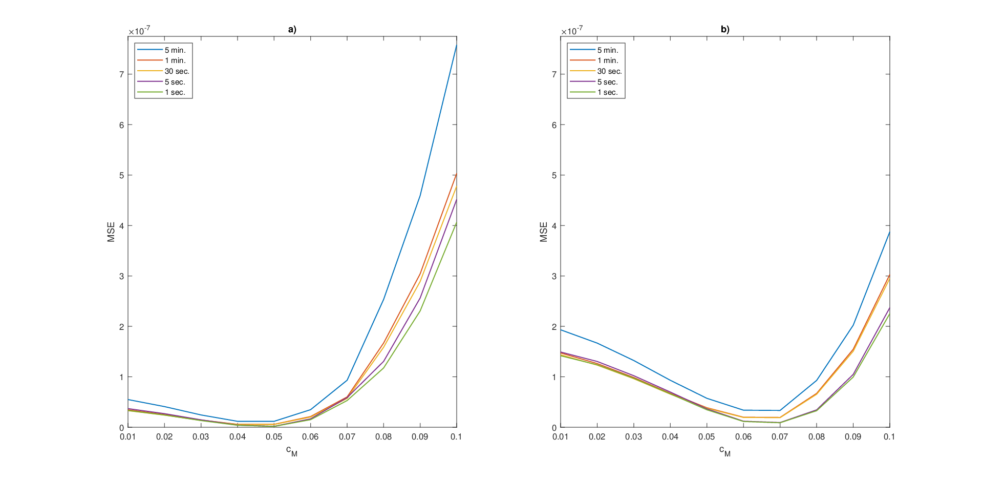
We assessed the finite-sample performance of the estimator (4) for increasing values of the sample size $n$ , in order to provide numerical support to Theorem 3.1. Specifically, we considered values of $\rho(n)=T/n$ ranging between $5$ minutes and $1$ second. For what concerns the frequency $N$ , which is needed for the convolution formula (2), we set $N=\left[c_{N}\rho(n)^{-1}\right]$ and selected $c_{N}=T/2$ . This selection yields the value of $N$ equal to the Nyquist frequency $[n/2]$ and allows obtaining the smallest variance of the asymptotic error, see (6) in Section 3. As for the frequency $M$ , we set $M=\left[c_{M}\rho(n)^{-1/2}\right]$ and optimized the value of the constant $c_{M}$ based on the (unfeasible) numerical minimization of the mean squared error (MSE). In this regard, we found that the MSE-optimal value of $c_{M}$ is equal to, resp., $0.05$ and $0.07$ for the models (15) and (16) (see also Subsection 4.3, where a feasible procedure to select $M$ is also discussed).

Table 1 illustrates the finite-sample performance of the estimator (4) under the two different data-generating processes considered. Specifically, Table 1 illustrates the MSE and the bias for the different values of the sampling frequency $\rho(n)$ . As expected, the bias and MSE improve as $n$ is increased for both the data-generating processes considered, thereby providing numerical support to Theorem 3.1. In particular, note that the performance of the estimator is still satisfactory for $\rho(n)$ equal to 5 minutes, the sampling frequency typically used in the absence of noise with empirical data. Additionally, it is worth mentioning that the estimator never produced negative volatility of volatility estimates in this simulation study.

	Heston model		stochastic vol-of-vol model
$\rho(n)$	MSE	Bias	MSE	Bias
5 minutes	$1.474\cdot 10^{-8}$	$-5.674\cdot 10^{-6}$	$3.886\cdot 10^{-8}$	$1.455\cdot 10^{-6}$
1 minute	$4.425\cdot 10^{-9}$	$-4.142\cdot 10^{-6}$	$1.939\cdot 10^{-8}$	$1.304\cdot 10^{-6}$
30 seconds	$2.913\cdot 10^{-9}$	$-3.801\cdot 10^{-6}$	$1.327\cdot 10^{-8}$	$1.269\cdot 10^{-6}$
5 seconds	$9.985\cdot 10^{-10}$	$-2.932\cdot 10^{-7}$	$8.113\cdot 10^{-9}$	$4.161\cdot 10^{-7}$
1 second	$4.229\cdot 10^{-10}$	$-1.833\cdot 10^{-7}$	$6.199\cdot 10^{-9}$	$3.644\cdot 10^{-7}$

Table 1: MSE and bias of the estimator (4) in correspondence of different values of

\rho(n)

. The true values of the daily integrated volatility of volatility are equal, on average, to

1.985\cdot 10^{-4}

and

3.957\cdot 10^{-4}

for, resp., the models (15) and (16).

As additional support to the results in Thereom 3.1, the q-q plots in Figures 1 and 2 offer a comparison between the empirical quantiles of the unfeasible standardized estimation error from Theorem 3.1 and the theoretical quantiles of a standard normal distribution for different values of $\rho(n)$ . Both in the case of the model (15) and the model (16), as $\rho(n)$ becomes smaller, the approximation to the the standard normal distribution improves. In particular, while the approximation of the body of the distribution is satisfactory also for the largest $\rho(n)$ considered, i.e., $5$ minutes, the approximation in the tails becomes accurate for $\rho(n)$ smaller or equal than $5$ seconds.

Refer to caption — Figure 1: Comparison, for different values of $\rho(n)$ , between the empirical quantiles of the standardized estimation error from Theorem 3.1, computed with simulated observations from the model (15), and the theoretical quantiles of a standard normal distribution.

4.3 Sensitivity to the frequency $M$

The careful selection of the frequency $M$ , that is, the constant $c_{M}$ , is key to efficiently implement the estimator (4) with finite samples. Given the selection $M=\left[c_{M}\rho(n)^{-1/2}\right]$ , Figure 3 shows the sensitivity of the MSE of the estimator to different values of the constant $c_{M}$ in the range $(0.01,1)$ , for different values of $\rho(n)$ . Based on Figure 3, the optimal MSE is achieved when $c_{M}$ is equal to, resp., $0.05$ and $0.07$ for the models (15) and (16), independently of $\rho(n)$ . Further, it appears that the MSE is relatively flat for $c_{M}$ in the intervals $(0.04,0.06)$ and $(0.06,0.07)$ .

As outlined in the following remark, it is possible to exploit the feasible Theorem 3.5 to optimize the selection of $c_{M}$ with empirical data.

Remark 4.1

The feasible selection of $c_{M}$ can be performed based on the adaptive procedure described in Section 2.4 of [Li et al., 2021]. For the estimator (4), the procedure can be summarized as follows. First, given an initial value for $c_{M}$ , denoted by $c_{M,0}$ , one computes the standard error of the estimator as $\rho(n)^{1/4}\sqrt{\Lambda_{n,N,M,L}}$ , exploiting the feasible estimator of the asymptotic variance in (12). Then, the computation of the standard error is iterated in correspondence of increasing values of $c_{M}$ on a grid of step size $s$ , that is, for $c_{M,j},\,j\geq 1,$ such that $c_{M,j}-c_{M,j-1}=s\,\,\,\forall j.$ Iterations stop when the absolute value of the marginal decrease in the standard error (w.r.t. the standard error recorded in correspondence to the initial value $c_{M,0}$ ) becomes smaller than a given threshold $\vartheta$ . Unreported simulations show that, for $L=n^{1/4}$ , the triple $(c_{M,0},s,\vartheta)=(0.03,0.01,0.25)$ provides an estimation accuracy which is comparable to that demonstrated in Subsection 4.2 with the unfeasible optimization of the MSE. Moreover, the same simulations suggest that the procedure is fairly robust to selections of the threshold $\vartheta$ in the interval $(0.2,0.3)$ .

4.4 Performance with irregular sampling

So far, in the simulation study we assumed that prices were observable on the equally-spaced grid with mesh size $\rho(n)$ equal to $1$ second. However, the setup of Section 3 allows for an irregular sampling scheme. To assess the robustness of the performance of the estimator (4) to irregular sampling, we considered the case when observation times follow a Poisson process, that is, durations between observations are drawn from an exponential distribution with mean $\lambda$ (see, e.g., [Mancino et al., 2017], Chapter $3.3$ ).

Specifically, we considered three different values of $\lambda$ , corresponding to an average duration $\delta$ of $1.25$ , $1.5$ and $2$ seconds, and compared the resulting MSE and bias values with the case of regular sampling on the 1-second grid. For the estimation with the Poisson scheme, we set $N=[n/2]$ and optimized $M$ based on the minimization of the MSE. In this regard, we found that it is MSE-optimal to select a smaller $M$ , compared to the regular-sampling case. Specifically, letting $M^{*}$ denote the optimal selection with regular 1-second sampling, numerical results suggest that it is optimal to select $M=[M^{*}/2]$ .

Table 2 reports the resulting bias and MSE, offering a comparison with the case where the a regular 1-second sampling scheme is adopted, corresponding to the last row of Table 1. The results in Table 2 suggest that the Fourier estimator (4) may still offer a satisfactory performance with irregular sampling schemes; in particular, it appears that the bias is relatively less affected than the MSE, compared to the regular-sampling case.

	Heston model		stochastic vol-of-vol model
$\delta$	MSE	Bias	MSE	Bias
$2$	$6.888\cdot 10^{-10}$	$-1.910\cdot 10^{-7}$	$9.672\cdot 10^{-9}$	$3.840\cdot 10^{-7}$
$1.5$	$5.250\cdot 10^{-10}$	$-1.888\cdot 10^{-7}$	$7.564\cdot 10^{-9}$	$3.776\cdot 10^{-7}$
$1.25$	$4.662\cdot 10^{-10}$	$-1.865\cdot 10^{-7}$	$6.696\cdot 10^{-9}$	$3.730\cdot 10^{-7}$
regular 1-sec. sampling	$4.229\cdot 10^{-10}$	$-1.833\cdot 10^{-7}$	$6.199\cdot 10^{-9}$	$3.644\cdot 10^{-7}$

Table 2: Comparison of MSE and bias of the estimator (4) when observation times follow a Poisson scheme (with different values of the average duration

\delta

) with the case of regular 1-second sampling.

4.5 Comparison with the performance of the rate-efficient realized estimator

This subsection contains a comparative study of the finite-sample performance of the rate-efficient Fourier estimator (4) and the rate-efficient realized estimator by [Ait-Sahalia and Jacod, 2014] (see Remark 3.2). We recall the definition of the latter. Let $\kappa(n)$ denote a sequence of integers such that $\kappa(n)\sim\beta\rho(n)^{-1/2}$ , $\beta>0,\,\rho(n):=T/n$ . The estimator reads

\displaystyle\hat{\gamma}^{2}_{n}=\frac{3}{2\kappa(n)}\sum_{i=1}^{n-2\kappa(n)+1}\Bigg(\Big(\widehat{\sigma}_{n}^{2}(t_{i+k(n)})-\widehat{\sigma}_{n}^{2}(t_{i})\Big)^{2}-\frac{4}{\kappa(n)}\big(\widehat{\sigma}_{n}^{2}(t_{i}\big))^{2}\Bigg),

(17)

where

\displaystyle\widehat{\sigma}_{n}^{2}(t_{i})=\frac{1}{\kappa(n)\rho(n)}\sum_{m=0}^{\kappa(n)-1}\Big(p(t_{i+m})-p(t_{i+m-1})\Big)^{2}

is the local estimator employed to pre-estimate the spot variance at time $t_{i}=i{T/n}$ , $i=0,...,n$ . The estimator (17) is also studied in [Vetter, 2015], where the author replaces $\big(\widehat{\sigma}_{n}^{2}(t_{i}\big))^{2}$ with

\displaystyle\widehat{\sigma}_{n}^{4}(t_{i})=\frac{1}{3\kappa(n)\rho(n)^{2}}\sum_{m=0}^{\kappa(n)-1}\Big(p(t_{i+m})-p(t_{i+m-1})\Big)^{4}.

(18)

The rate-efficient realized estimator considered in [Vetter, 2015] thus reads

\hat{\bar{\gamma}}^{2}_{n}=\frac{3}{2\kappa(n)}\sum_{i=1}^{n-2\kappa(n)+1}\Bigg(\Big(\widehat{\sigma}_{n}^{2}(t_{i+k(n)})-\widehat{\sigma}_{n}^{2}(t_{i})\Big)^{2}-\frac{4}{\kappa(n)}\widehat{\sigma}_{n}^{4}(t_{i})\Bigg).

(19)

For the comparison, we replicated the simulation study carried out in Subsection 4.2, this time using the realized estimators (17) and (19) to obtain estimates of the daily integrated volatility of volatility. The implementation of realized estimators requires the selection of the tuning parameter $\beta$ . After setting $\kappa(n)=[\beta\rho(n)^{-1/2}]$ , we selected $\beta=0.04$ (resp., $\beta=0.06$ ) in the case of the model (15) (resp., 16), based on the unfeasible optimization of the MSE with 1-second samples. Tables 3 and 4 summarize the results. By comparing the latter with Table 1 in Subsection 4.2, it is immediate to see that the performance of the realized estimators (17) and (19) is not satisfactory, both in terms of bias and MSE, compared to the case of the Fourier estimator (4). See also [Sanfelici et al., 2015] and [Toscano and Recchioni, 2021] for similar considerations on the finite-sample performance of realized volatility of volatility estimators. Moreover, note that the comparison for $\rho(n)$ equal to $5$ minutes is omitted, since the resulting bias and MSE of the realized estimators are larger than $1$ in absolute value. Finally, simulations suggest that the use of the quarticity estimator in the de-biasing term in (19) does not improve the finite-sample performance.

	Heston model		stochastic vol-of-vol model
$\rho(n)$	MSE	Bias	MSE	Bias
1 minute	$1.800\cdot 10^{-3}$	$1.473\cdot 10^{-2}$	$1.655\cdot 10^{-3}$	$1.299\cdot 10^{-2}$
30 seconds	$5.364\cdot 10^{-4}$	$1.388\cdot 10^{-2}$	$4.114\cdot 10^{-4}$	$1.119\cdot 10^{-2}$
5 seconds	$3.733\cdot 10^{-4}$	$1.047\cdot 10^{-2}$	$3.390\cdot 10^{-4}$	$1.001\cdot 10^{-2}$
1 second	$3.322\cdot 10^{-4}$	$9.838\cdot 10^{-3}$	$2.999\cdot 10^{-4}$	$9.555\cdot 10^{-3}$

Table 3: MSE and bias of the estimator (17) in correspondence of different values of

\rho(n)

. The true values of the daily integrated volatility of volatility are equal, on average, to

1.985\cdot 10^{-4}

and

3.957\cdot 10^{-4}

for, resp., the models (15) and (16).

	Heston model		stochastic vol-of-vol model
$\rho(n)$	MSE	Bias	MSE	Bias
1 minute	$1.501\cdot 10^{-3}$	$1.575\cdot 10^{-2}$	$1.377\cdot 10^{-3}$	$1.303\cdot 10^{-2}$
30 seconds	$5.461\cdot 10^{-4}$	$1.456\cdot 10^{-2}$	$4.336\cdot 10^{-4}$	$1.122\cdot 10^{-2}$
5 seconds	$3.783\cdot 10^{-4}$	$1.091\cdot 10^{-2}$	$3.302\cdot 10^{-4}$	$9.998\cdot 10^{-3}$
1 second	$3.324\cdot 10^{-4}$	$9.840\cdot 10^{-3}$	$3.002\cdot 10^{-4}$	$9.555\cdot 10^{-3}$

Table 4: MSE and bias of the estimator (19) in correspondence of different values of

\rho(n)

. The true values of the daily integrated volatility of volatility are equal, on average, to

1.985\cdot 10^{-4}

and

3.957\cdot 10^{-4}

for, resp., the models (15) and (16).

Remark 4.2

Unreported simulations show that the realized estimators (17) and (19) improve their finite-sample performance for larger values of the estimation horizon $T$ . Specifically, realized estimators appear to achieve satisfactory accuracy, compared to the Fourier estimator (4), when $T$ is equal to one year. This is in line with the selection of $T$ equal to one year in the numerical and empirical high-frequency exercises by [Li et al., 2021], where the performance of the noise- and jump-robust version of the realized estimator volatility of volatility estimator is investigated.

5 Empirical analysis

To the best of our knowledge, the empirical properties of the volatility of volatility of financial assets have been scarcely explored in the literature. The aim of the empirical study presented in this section is thus to provide insight into the existence of stylized facts pertaining to the daily dynamics of the volatility of volatility.

In fact, the numerical evidence presented in Section 4 suggests that the Fourier methodology allows reconstructing the integrated volatility of volatility with satisfactory accuracy on daily intervals by means of the rate-efficient estimator (4). Accordingly, in this section we use the estimator (4) to obtain the daily volatility of volatility series for two market indices: the S&P500 and the EUROSTOXX50. The periods considered for the analysis are, resp., May 1, 2007 - August 6, 2021 and June 29, 2005 - May 28, 2021.

5.1 Data description, estimation and sample statistics

For the empirical analysis we used the series of $5$ -minute trade prices, recorded during trading hours. Specifically, for the S&P500 index, we used the prices recorded between $9.30$ a.m. and $4$ p.m., while for the EUROSTOXX50 index we employed the prices recorded between $9$ a.m. and $5.30$ p.m. Days with early closure were discarded.

The estimation of the daily integrated volatility of volatility was performed via the rate-efficient Fourier estimator (4), without considering overnight returns. Before performing the estimation, we run the test by [Ait-Sahalia and Xiu 2014] on 5-minute series and found that the assumption of absence of noise could not be rejected at the $5\%$ significance level for both indices. Moreover, following [Wang and Mykland, 2014], days with jumps were removed, based on the results of the test by [Lee and Mykland, 2008], which was applied at the $1\%$ significance level. Overall, the number of days for which we estimated the volatility of volatility is $3343$ and $3522$ for, resp., the S&P500 and EUROSTOXX50.

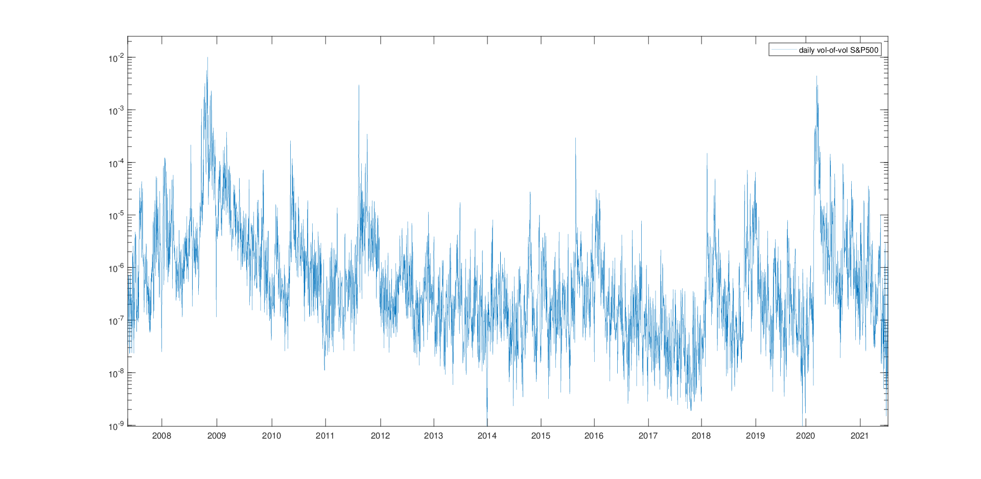
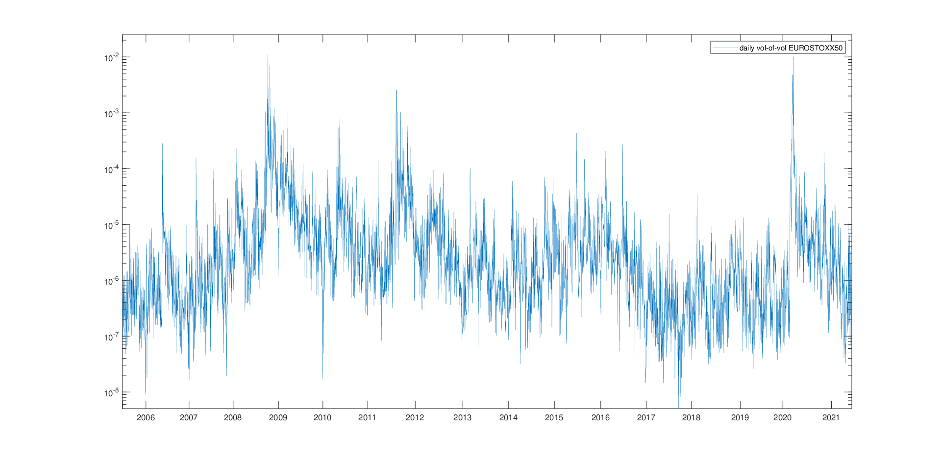
For the estimation, given the choice of the sampling frequency $\rho(n)=5$ minutes, we set $N=[c_{N}\rho(n)^{-1}]$ and $M=[c_{M}\rho(n)^{-1/2}]$ . Then we selected $c_{N}$ such that $N$ equals the Nyquist frequency (see Subsection 4.2) and $c_{M}$ based on the feasible procedure illustrated in Subsection 4.3. The resulting values of $c_{M}$ are equal, on average, to $0.054$ and $0.065$ for, resp., the S&P500 and the EUROSTOXX50. Figures 4 and 5 display the reconstructed trajectories of the daily volatility of volatility of the two indices, while Table 5 compares sample statistics of volatility and volatility of volatility estimates. Daily volatility estimates were obtained via the Fourier estimator by [Malliavin and Mancino, 2002], applied to 5-minute returns³³ 3 All the analyses appearing in this section and involving the computation of the volatility were also performed using volatility estimates obtained via the 5-minute realized variance and the final outcome was pretty much the same.. We note that all volatility of volatility estimates obtained are strictly positive.

daily series	mean	median	st. dev.	min	max	skew.	kurt.
SPX vol.	$8.598\cdot 10^{-5}$	$3.098\cdot 10^{-5}$	$2.152\cdot 10^{-4}$	$1.701\cdot 10^{-6}$	$3.209\cdot 10^{-3}$	$7.951$	$83.902$
SPX vol. of vol.	${\color[rgb]{0,0,0}2.351}\cdot 10^{-5}$	${\color[rgb]{0,0,0}3.867}\cdot 10^{-7}$	${\color[rgb]{0,0,0}2.608}\cdot 10^{-4}$	${\color[rgb]{0,0,0}9.545\cdot 10^{-10}}$	${\color[rgb]{0,0,0}1.009}\cdot 10^{-2}$	${\color[rgb]{0,0,0}24.442}$	${\color[rgb]{0,0,0}780.377}$
ESTX vol.	$1.093\cdot 10^{-4}$	$5.848\cdot 10^{-5}$	$1.944\cdot 10^{-4}$	$2.845\cdot 10^{-6}$	$3.916\cdot 10^{-3}$	$8.198$	$104.168$
ESTX vol. of vol.	${\color[rgb]{0,0,0}3.233}\cdot 10^{-5}$	${\color[rgb]{0,0,0}1.841}\cdot 10^{-6}$	${\color[rgb]{0,0,0}3.267}\cdot 10^{-4}$	${\color[rgb]{0,0,0}5.054\cdot 10^{-9}}$	${\color[rgb]{0,0,0}1.630}\cdot 10^{-2}$	${\color[rgb]{0,0,0}24.726}$	${\color[rgb]{0,0,0}727.501}$

Table 5: Sample statistics (mean, median, standard deviation, minimum, maximum, skewness, kurtosis) of the estimated daily integrated volatility and volatility of volatility of the S&P500 (SPX) and the EUROSTOXX50 (ESTX) indices over, resp., the periods May 1, 2007- August 6, 2021 and June 29, 2005 - May 28, 2021.

Figures 4 and 5 show that the volatility of volatility spikes during financial crises, while remaining rather low and stable during tranquil periods. Indeed, both daily series reach their three highest peaks in correspondence of, resp., the global financial crisis starting at the end of 2008, the instabilities of the Euro area in the second part of 2011 and the outbreak of the COVID pandemic in the first months of 2020.

Moreover, based on Table 5, we make the following remarks. First, the volatility of volatility is on average smaller than the volatility in the case of both indices. Secondly, the volatility of volatility appears to be more volatile than the volatility itself, as it displays larger sample standard deviations and maxima for both the estimated series. Finally, the volatility of volatility appears to be much more skewed and leptokurtic than the volatility for both the indices.

An analysis of the empirical regularities displayed by the reconstructed daily series of the volatility of volatility of the S&P500 and the EUROSTOXX50 is illustrated in the next subsection.

5.2 Insight into volatility-of-volatility stylized facts

The literature on the stylized facts related to the behavior of the volatility of financial assets is very rich (see, for instance, [Andersen et al., 2001], [Patton and Engle, 2001] and [Corsi, 2009], among many others). These include, e.g., clustering, long memory, mean-reversion, log-normality and leverage effects. Nowadays, the volatility can be regarded, in some sense, as a traded asset itself. In fact, it is possible to “trade” the volatility of many financial asset classes via quoted and O.T.C. volatility derivatives (e.g., variance swaps, VIX futures and VIX options). Therefore, it may be of interest to evaluate which typical features of the daily volatility actually apply to the daily volatility of the volatility itself.

We have already observed in the previous subsection that the volatility of volatility shows clusters, being larger in correspondence of crises and smaller and less volatile during periods of economic stability. However, based on the observation of the sample auto-correlation function (see Figures 6 and 7), it appears to be less persistent than the volatility for both the indices considered. As for the mean-reversion property, the Augmented Dickey-Fuller test rejects the hypothesis of a unit root for both volatility of volatility series analyzed, at the $0.01\%$ significance level.

We also examined the year-by-year correlation of the daily volatility of volatility with, resp., the daily volatility and the daily log-return, computed as the difference between the closing and opening log-price. The dynamics of such correlations are summarized in Tables 6 and 7, where the values of return-variance correlations, a rough proxy of the leverage effect, are also displayed for comparison⁴⁴ 4 Note that the correlations appearing in Tables 6 and 7 are typically pushed towards zero by the presence of a finite-sample bias, see [Ait-Sahalia et al., 2013]. For this reason, their true values are likely to be larger, in absolute value. However, obtaining unbiased and efficient estimates of these correlations goes beyond the scope of the exploratory analysis proposed.. For both the indices, we observe that the yearly correlation between the log-return and the volatility of volatility tends to be negative and to follow the return-variance correlation closely, although being most often smaller in absolute value. This result may suggest the existence of a “second-order” leverage effect: what we observe is in fact that when the asset price decreases, not only the volatility increases, due the asset becoming riskier, but also the volatility of volatility - which can be seen as a proxy of the uncertainty about the amount of risk perceived by market operators, that is, the “volatility of risk” - becomes larger. The yearly correlation between the volatility of volatility and the volatility is instead positive and close to $0.7$ on average for both the indices. This is consistent with the presence of volatility-of-volatility peaks in periods of higher market volatility.

year	vol. of vol. - vol.	vol.- ret.	vol. of vol. - ret.
2007	0.730	-0.126	-0.030
2008	0.689	0.049	0.054
2009	0.727	-0.063	0.067
2010	0.827	-0.199	-0.073
2011	0.728	0.019	0.213
2012	0.686	-0.231	0.022
2013	0.706	-0.354	-0.129
2014	0.842	-0.140	0.030
2015	0.582	-0.153	-0.281
2016	0.849	-0.122	-0.151
2017	0.638	-0.348	-0.160
2018	0.758	-0.218	-0.125
2019	0.858	-0.125	-0.026
2020	0.821	0.090	0.172
2021	0.913	-0.305	-0.219
average	0.757	-0.147	-0.043

Table 6: S&P500 index: sample yearly correlations of the daily volatility of volatility with the corresponding daily volatility and daily log-return.

year	vol. of vol. - vol.	vol.- ret.	vol. of vol. - ret.
2005	0.6906	-0.1463	-0.1740
2006	0.593	-0.119	-0.101
2007	0.689	-0.237	-0.252
2008	0.833	-0.130	-0.053
2009	0.621	-0.144	-0.009
2010	0.804	-0.107	-0.040
2011	0.864	-0.072	-0.156
2012	0.718	-0.035	0.023
2013	0.685	-0.141	-0.052
2014	0.742	-0.128	-0.074
2015	0.584	-0.111	0.052
2016	0.732	-0.327	-0.275
2017	0.552	-0.172	-0.196
2018	0.791	-0.327	-0.303
2019	0.743	-0.180	-0.016
2020	0.705	-0.276	-0.084
2021	0.762	-0.185	-0.081
average	0.712	-0.167	-0.105

Table 7: EUROSTOXX50 index: sample yearly correlations of the daily volatility of volatility with the corresponding daily volatility and daily log-return.

Finally, we test for the Gaussianity of the logarithmic volatility and volatility of volatility estimates, using the Jarque-Bera and Anderson-Darling tests at the $5\%$ significance level. The years in which both tests reject the null hypothesis of Gaussianity are 2008, 2011, 2016 and 2020, that is, the years in the sample that were the most characterized by market turmoil (in order: the global financial crisis, the Euro-area instability phase, Brexit and the outbreak of the COVID pandemic). This happens for both the quantities tested and both the indices analyzed, thus suggesting that the log-normal approximation for the distribution of the volatility and the volatility of volatility is more satisfactory in periods of market stability.

6 Conclusions

This paper fills a gap in the literature on financial econometrics by deriving the convergence rate of the Fourier estimator of the volatility of volatility. In this regard, we showed that the bias-corrected version of the estimator reaches the optimal rate $n^{1/4}$ , while the estimator without bias-correction achieves a sub-optimal rate, but has a smaller asymptotic variance.

Further, we presented a numerical study that shows that the rate-optimal Fourier estimator of the volatility of volatility performs well in finite samples, even at the relatively small daily estimation horizon, where the competing rate-efficient realized estimator shows a poor performance.

Finally, we applied the Fourier estimator to multi-year samples of S&P500 and EUROSTOXX50 observations and gained some new knowledge about the empirical regularities that characterize the daily dynamics of the volatility of volatility, a topic which so far had been scarcely explored in the literature.

7 Appendix A: proofs

The proofs of Theorems 3.1, 3.5, 3.6 and 3.7 are illustrated in the next subsections. Some preliminary remarks are useful.

Remark 7.1

As every continuous process is locally bounded, all processes appearing in the proofs are locally bounded. Moreover, standard localization procedures (see, e.g., [Ait-Sahalia and Jacod, 2014]) allow assuming that any locally bounded process is actually bounded and almost-surely positive processes can be considered as bounded away from zero.

Remark 7.2

In [Malliavin and Mancino, 2009], Lemma 2.2, it is proved that the drift component of the semi-martingale model gives no contribution to the convolution formula (2). Therefore, we will refer to the drift-less model in Assumption (A.I). Moreover, as observed in [Malliavin and Mancino, 2002], we can assume that $p(0)=p(2\pi)$ and $v(0)=v(2\pi)$ . In fact, if $p(0)\not=p(2\pi)$ (similarly for the process $v$ ), we introduce

\widetilde{p}(t)=p(t)-{t\over{2\pi}}[p(2\pi)-p(0)].

Then, while $\widetilde{p}$ satisfies the required assumption, at the same time the volatility and co-volatilities estimations are not affected by a modification of the drift as above. From the point of view of the modeling, we may consider

d\widetilde{p}(t)=\sqrt{v(t)}dW(t),

d\widetilde{v}(t)=\gamma(t)\,dZ(t),

being $v(t)=\widetilde{v}(t)-{t\over{2\pi}}[{\widetilde{v}}(2\pi)-{\widetilde{v}}(0)].$ In fact, for any $k\not=0$ , it holds $c_{k}(dv)=c_{k}(d\widetilde{v})$ , while the $0$ -th Fourier coefficient, $c_{0}(dv)$ , is not contributing to the definition of the Fourier estimator of the volatility of volatility. The situation would change in the case when one wishes to estimate the spot volatility. However, this is not an issue of the present study, as the estimation of the spot volatility is not required.

7.1 Preliminary decomposition

Given the discrete time observations $\{0=t_{0}\leq\ldots\leq t_{i}\leq\ldots\leq t_{n}=2\pi\}$ , we use the notation in continuous time by letting $\varphi_{n}(t):=\sup\{t_{j}:t_{j}\leq t\}$ , for the sake of simplicity. From the Itô formula we have the following decomposition of the term (2)

c_{k}(v_{n,N}):=A_{k,n}+B_{k,n,N}+C_{k,n,N},

(20)

where

A_{k,n}:={1\over{2\pi}}\int_{0}^{2\pi}e^{-ik\varphi_{n}(s)}v(s)ds,

(21)

B_{k,n,N}:={1\over{2\pi}}\int_{0}^{2\pi}e^{-ik\varphi_{n}(s)}\int_{0}^{s}D_{N}(\varphi_{n}(s)-\varphi_{n}(u))\sigma(u)dW_{u}\,\sigma(s)dW_{s},

(22)

C_{k,n,N}:={1\over{2\pi}}\int_{0}^{2\pi}\int_{0}^{s}e^{-ik\varphi_{n}(u)}D_{N}(\varphi_{n}(s)-\varphi_{n}(u))\sigma(u)dW_{u}\,\sigma(s)dW_{s}.

(23)

It follows that (3) is equal to the following sum:

{2\pi\over{M+1}}\sum_{|k|\leq M}\left(1-{|k|\over{M+1}}\right)k^{2}\,A_{k,n}A_{-k,n}

(24)

+{2\pi\over{M+1}}\sum_{|k|\leq M}\left(1-{|k|\over{M+1}}\right)\,k^{2}\,2(A_{k,n}B_{-k,n,N}+A_{k,n}C_{-k,n,N})

(25)

+{2\pi\over{M+1}}\sum_{|k|\leq M}\left(1-{|k|\over{M+1}}\right)\,k^{2}\,(B_{k,n,N}B_{-k,n,N}+2B_{k,n,N}C_{-k,n,N}+C_{k,n,N}C_{-k,n,N}).

(26)

Throughout the proofs, we denote

Y_{n,N}(t,s):=\int^{t}_{0}D_{N}(\varphi_{n}(s)-\varphi_{n}(u))\sigma(u)dW_{u}

(27)

and, for brevity, we will use the following notation for the Dirichlet and the Fejér kernels (see also the Appendix B):

D_{N,n}(s-u):=D_{N}(\varphi_{n}(s)-\varphi_{n}(u)),\ \ \ \ F_{M,n}(s-u):=F_{M}(\varphi_{n}(s)-\varphi_{n}(u)).

(28)

Similarly, for the derivatives of the Fejér kernel⁵⁵ 5 We stress the point that the notation $D_{N,n}(s-u)$ refers to $D_{N}(\varphi_{n}(s)-\varphi_{n}(u))$ , which is a function of two time variables, $(s,u)$ , as stated in (28). It is not to identify it with $D_{N}(\varphi_{n}(s-u))$ . Notation (28) is maintained in order to highlight the role of the convolution product, which is the main characteristic of the Fourier estimation method in [Malliavin and Mancino, 2009]. we will use $F^{\prime}_{M,n}$ and $F^{\prime\prime}_{M,n}$ .

In order to identify the different contribution of all terms, we start with equation (24), which can be written as

{2\pi\over{M+1}}\sum_{|k|\leq M}\left(1-{|k|\over{M+1}}\right)\,k^{2}c_{k}(v)c_{-k}(v)

(29)

+{2\pi\over{M+1}}\sum_{|k|\leq M}\left(1-{|k|\over{M+1}}\right)k^{2}\,\left(A_{k,n}A_{-k,n}-c_{k}(v)c_{-k}(v)\right).

(30)

We consider now the term (25). An application of the Itô formula shows that it is equal to

2(AB^{(i)}_{M,n,N}+AB^{(ii)}_{M,n,N}+AC^{(i)}_{M,n,N}+AC^{(ii)}_{M,n,N}),

where

AB^{(i)}_{M,n,N}:={1\over{2\pi}}\int_{0}^{2\pi}\int_{0}^{s}{1\over{M+1}}\sum_{|k|\leq M}\left(1-{|k|\over{M+1}}\right)k^{2}e^{{\rm i}k(\varphi_{n}(s)-\varphi_{n}(u))}v(u)du\,Y_{n,N}(s,s)\sigma(s)dW_{s}

=-\int_{0}^{2\pi}{1\over{2\pi}}\int_{0}^{s}{1\over{M+1}}F_{M,n}^{\prime\prime}(s-u)v(u)du\,Y_{n,N}(s,s)\sigma(s)dW_{s},

(31)

AB^{(ii)}_{M,n,N}:=\int_{0}^{2\pi}{1\over{2\pi}}\int_{0}^{s}{1\over{M+1}}\sum_{|k|\leq M}\left(1-{|k|\over{M+1}}\right)k^{2}e^{-{\rm i}k(\varphi_{n}(s)-\varphi_{n}(u))}\,Y_{n,N}(u,s)\sigma(u)dW_{u}\,v(s)ds

=-\int_{0}^{2\pi}{1\over{2\pi}}\int_{0}^{s}{1\over{M+1}}F_{M,n}^{\prime\prime}(s-u)\,Y_{n,N}(u,s)\,\sigma(u)dW_{u}\,v(s)ds,

(32)

and, letting

Y_{k,n,N}(t,s):=\int_{0}^{t}e^{-{\rm i}k\varphi_{n}(u)}D_{N}(\varphi_{n}(s)-\varphi_{n}(u))\sigma(u)dW_{u},

then

AC^{(i)}_{M,n,N}:={1\over{M+1}}\sum_{|k|\leq M}\left(1-{|k|\over{M+1}}\right)k^{2}{1\over{2\pi}}\int_{0}^{2\pi}\int_{0}^{s}e^{-{\rm i}k\varphi_{n}(u)}v(u)du\,Y_{-k,n,N}(s,s)\sigma(s)dW_{s}

=-\int_{0}^{2\pi}{1\over{2\pi}}\int_{0}^{s}\int_{0}^{u}{1\over{M+1}}F_{M,n}^{\prime\prime}(u-u_{1})D_{N,n}(s-u_{1})\sigma(u_{1})dW_{u_{1}}\,v(u)du\,\sigma(s)dW_{s}

(33)

-\int_{0}^{2\pi}{1\over{2\pi}}\int_{0}^{s}\int_{0}^{u}{1\over{M+1}}F_{M,n}^{\prime\prime}(u-u_{1})v(u_{1})du_{1}D_{N,n}(s-u)\sigma(u)dW_{u}\,\sigma(s)dW_{s},

(34)

and

AC^{(ii)}_{M,n,N}:={1\over{M+1}}\sum_{|k|\leq M}\left(1-{|k|\over{M+1}}\right)k^{2}{1\over{2\pi}}\int_{0}^{2\pi}\int_{0}^{s}Y_{-k,n,N}(s_{1},s)\sigma(s_{1})dW_{s_{1}}\,e^{-{\rm i}k\varphi_{n}(s)}v(s)ds

=-\int_{0}^{2\pi}{1\over{M+1}}{1\over{2\pi}}\int_{0}^{s}\int_{0}^{s^{\prime}}F_{M,n}^{\prime\prime}(s-u)D_{N,n}(s-u)\,\sigma(u)dW_{u}\,\sigma(s_{1})dW_{s_{1}}\,v(s)ds.

(35)

Finally, we consider the term (26). Using the fact that the Fejér kernel is an even function, it can be re-written as

{2\pi\over{M+1}}\sum_{|k|\leq M}\left(1-{|k|\over{M+1}}\right)\,k^{2}\,(B_{k,n,N}B_{-k,n,N}+2B_{k,n,N}C_{-k,n,N}+C_{k,n,N}C_{-k,n,N})

=BB_{M,n,N}^{(i)}+2BB_{M,n,N}^{(ii)}+2(BC_{M,n,N}^{(i)}+BC_{M,n,N}^{(ii)}+BC_{M,n,N}^{(iii)})+CC_{M,n,N}^{(i)}+2CC_{M,n,N}^{(ii)},

where, using the notation introduced in (27), each term is defined as follows:

BB_{M,n,N}^{(i)}:={1\over{2\pi}}{1\over{M+1}}\sum_{|k|\leq M}\left(1-{|k|\over{M+1}}\right)k^{2}\int_{0}^{2\pi}Y_{n,N}^{2}(s,s)v(s)ds,

(36)

BB_{M,n,N}^{(ii)}:=-\int_{0}^{2\pi}{1\over{2\pi}}\int_{0}^{u}{1\over{M+1}}F^{\prime\prime}_{M,n}(u-s)Y_{n,N}(s,s)\sigma(s)dW_{s}Y_{n,N}(u,u)\sigma(u)dW_{u},

(37)

BC_{M,n,N}^{(i)}:=-\int_{0}^{2\pi}{1\over{2\pi}}\int_{0}^{s}{1\over{M+1}}F^{\prime\prime}_{M,n}(s-v)D_{N,n}(s-v)\sigma(v)dW_{v}\,Y_{n,N}(s,s)v(s)ds,

(38)

BC_{M,n,N}^{(ii)}:={1\over{M+1}}\sum_{|k|\leq M}\left(1-{|k|\over{M+1}}\right)k^{2}{1\over{2\pi}}\int_{0}^{2\pi}\,\int_{0}^{u}e^{-ik\phi_{n}(s)}Y_{n,N}(s,s)\sigma(s)dW_{s}\,Y_{k,n,N}(u,u)\,\sigma(u)dW_{u},

(39)

BC_{M,n,N}^{(iii)}:=-\int_{0}^{2\pi}\int_{0}^{u}{1\over{2\pi}}\int_{0}^{v}{1\over{M+1}}F^{\prime\prime}_{M,n}(v-s)D_{N,n}(v-s)\sigma(s)dW_{s}\,\sigma(v)dW_{v}\,Y_{N,n}(u,u)\sigma(u)dW_{u},

(40)

CC_{M,n,N}^{(i)}:={1\over{2\pi}}{1\over{M+1}}\sum_{|k|\leq M}\left(1-{|k|\over{M+1}}\right)k^{2}\int_{0}^{2\pi}Y_{k,n,N}(s,s)Y_{-k,n,N}(s,s)v(s)ds,

(41)

CC_{M,n,N}^{(ii)}:={1\over{M+1}}\sum_{|k|\leq M}\left(1-{|k|\over{M+1}}\right)k^{2}{1\over{2\pi}}\int_{0}^{2\pi}\int_{0}^{s}Y_{k,n,N}(v,v)\sigma(v)dW_{v}\,Y_{-k,n,N}(s,s)\sigma(s)dW_{s}.

(42)

In summary, the estimation error

\widehat{\gamma}^{2}_{n,N,M}-{1\over{2\pi}}\int_{0}^{2\pi}\gamma^{2}(t)dt

(43)

comprises the study of four main components:

{2\pi\over{M+1}}\sum_{|k|\leq M}\left(1-{|k|\over{M+1}}\right)\,k^{2}c_{k}(v)c_{-k}(v)-{\frac{1}{2\pi}}\int_{0}^{2\pi}\gamma^{2}(t)dt

(44)

+{2\pi\over{M+1}}\sum_{|k|\leq M}\left(1-{|k|\over{M+1}}\right)k^{2}\,\left(A_{k,n}A_{-k,n}-c_{k}(v)c_{-k}(v)\right)

(45)

+2\,(AB^{(i)}_{M,n,N}+AB^{(ii)}_{M,n,N}+AC^{(i)}_{M,n,N}+AC^{(ii)}_{M,n,N}+BB_{M,n,N}^{(ii)}+BC_{M,n,N}^{(ii)}+BC_{M,n,N}^{(iii)}+CC_{M,n,N}^{(ii)})

(46)

+BB_{M,n,N}^{(i)}+2BC_{M,n,N}^{(i)}+CC_{M,n,N}^{(i)}-K\widehat{\sigma}^{4}_{n,N,M},

(47)

where $\widehat{\sigma}^{4}_{n,N,M}$ is defined in (5) and the constant $K$ is determined in (51).

Accordingly, the proof of the theorem is divided into four steps. The first and second steps comprise the study of the bias correction term (47) and the asymptotic negligibility of the discretization error (45). The other two steps follow [Jacod, 1997] in order to identify the asymptotic variance and prove the stable convergence in law.

In the proof we consider the case of regular sampling, i.e., $\varphi_{n}(t)={2\pi\over n}j$ , if ${2\pi\over n}j\leq t<{2\pi\over n}(j+1)$ , $j=0,\ldots,n$ . Further, $C$ will always denote a positive constant, not necessarily the same.

7.2 Step I. The bias-correction term

Firstly, we show that the term (47) is $o_{p}(\rho(n)^{1/4})$ , therefore proving that the error (43) is equal to

{2\pi\over{M+1}}\sum_{|k|\leq M}\left(1-{|k|\over{M+1}}\right)\,k^{2}c_{k}(v)c_{-k}(v)-{\frac{1}{2\pi}}\int_{0}^{2\pi}\gamma^{2}(t)dt

+{2\pi\over{M+1}}\sum_{|k|\leq M}\left(1-{|k|\over{M+1}}\right)k^{2}\,\left(A_{k,n}A_{-k,n}-c_{k}(v)c_{-k}(v)\right)

+2\,(AB^{(i)}_{M,n,N}+AB^{(ii)}_{M,n,N}+AC^{(i)}_{M,n,N}+AC^{(ii)}_{M,n,N}+BB_{M,n,N}^{(ii)}+BC_{M,n,N}^{(ii)}+BC_{M,n,N}^{(iii)}+CC_{M,n,N}^{(ii)})

+o_{p}(\rho(n)^{1/4}).

We begin by studying the term $BB_{M,n,N}^{(i)}$ defined by (36). The term $BC_{M,n,N}^{(i)}$ defined by (38) and the term $CC_{M,n,N}^{(i)}$ defined by (41) are analogous to $BB_{M,n,N}^{(i)}$ and give the same contribution.

Using the Itô formula, the term

BB_{M,n,N}^{(i)}:={1\over{M+1}}\sum_{|k|\leq M}\left(1-{|k|\over{M+1}}\right)k^{2}{1\over{2\pi}}\int_{0}^{2\pi}Y_{n,N}^{2}(s,s)v(s)ds

reads as

{1\over{M+1}}\sum_{|k|\leq M}\left(1-{|k|\over{M+1}}\right)k^{2}{1\over{2\pi}}\int_{0}^{2\pi}\int_{0}^{s}D_{N,n}^{2}(s-u)v(u)du\,v(s)ds

(48)

+{1\over{M+1}}\sum_{|k|\leq M}\left(1-{|k|\over{M+1}}\right)k^{2}{1\over{2\pi}}\int_{0}^{2\pi}2\int_{0}^{s}Y_{n,N}(u,s)D_{N,n}(s-u)\sigma(u)dW_{u}\,v(s)ds.

(49)

The leading term is the first one, namely (48), which is easily seen to be equal to

{1\over{M+1}}{1\over{6}}M(M+1)(M+2)\,{1\over{2\pi}}\int_{0}^{2\pi}\,\int_{0}^{s}D_{N,n}^{2}(s-u)v(u)du\,v(s)ds.

(50)

Now, using Lemma 8.2 and noting that $N/n\sim c_{N}/(2\pi)$ and $M^{2}/n\sim c^{2}_{M}/(2\pi)$ , we have that (50) converges in probability to

{c_{M}^{2}\over{{\color[rgb]{0,0,0}12}}}\,(1+2\eta({c_{N}/\pi})){1\over{2\pi}}\int_{0}^{2\pi}\sigma^{4}(t)dt.

Consider now (49). Exploiting the boundedness of the process $v$ , it is enough to observe that

E\left[\left(\int_{0}^{s}Y_{n,N}(u,s)D_{N,n}(s-u)\sigma(u)dW_{u}\right)^{2}\right]=E\left[\int_{0}^{s}Y^{2}_{n,N}(u,s)D^{2}_{N,n}(s-u)v(u)du\right]

\leq C\,\int_{0}^{s}\int_{0}^{u}D^{2}_{N,n}(s-s_{1})ds_{1}\,D^{2}_{N,n}(s-u)du=O(\rho(n)^{3}),

where we have used Lemma 8.2 and the property that $D^{2}_{N,n}(s-s_{1})\leq CN^{-2}$ for $s_{1}<s-\varepsilon$ , $\varepsilon>0$ , for $n$ large enough. Therefore, in probability the term (49) has order $M^{2}\rho(n)^{3/2}\sim c_{M}^{2}\rho(n)^{-1}\rho(n)^{3/2}=c_{M}^{2}\rho(n)^{1/2}$ , and thus it converges to zero.

Finally, let

K:=\left({1\over{{\color[rgb]{0,0,0}12}}}+{2\over{{\color[rgb]{0,0,0}12}}}+{1\over{{\color[rgb]{0,0,0}12}}}\right)\,{c_{M}^{2}\over{2\pi}}(1+2\eta(c_{N}/\pi))={{\color[rgb]{0,0,0}1}\over{3}}\,{c_{M}^{2}\over{2\pi}}(1+2\eta(c_{N}/\pi)).

(51)

Then, following [Livieri et al., 2019], Theorem 3, the following convergence in probability holds:

\rho(n)^{-1/2}\left(K\hat{\sigma}^{4}_{n,N,M}-(BB_{M,n,N}^{(i)}+2BC_{M,n,N}^{(i)}+CC_{M,n,N}^{(i)})\right)\to K(X_{c_{M}}+Y_{c_{M},c_{N}}),

where $X_{c_{M}}$ are $Y_{c_{M},c_{N}}$ are defined as

X_{c_{M}}:=-{1\over c_{M}}{1\over\pi}\int_{0}^{2\pi}\gamma^{2}(t)dt,\ \ \ \ Y_{c_{M},c_{N}}:=2c_{M}{1\over\pi}(1+2\eta(c_{N}/\pi))\int_{0}^{2\pi}\sigma^{4}(t)dt.

Therefore, the proof that (47) is $o_{p}(\rho(n)^{1/4})$ is complete.

7.3 Step II. The statistical error

In this paragraph we consider the discretization error component (45), which reads as

{1\over{M+1}}{1\over{2\pi}}\left(\int_{0}^{2\pi}2\int_{0}^{s}F_{M,n}^{\prime\prime}(s-u)v(u)du\,v(s)ds-\int_{0}^{2\pi}2\int_{0}^{s}F_{M}^{\prime\prime}(s-u)v(u)du\,v(s)ds\right)

={1\over{M+1}}{1\over{2\pi}}\int_{0}^{2\pi}2\int_{0}^{s}\left(F_{M,n}^{\prime\prime}(s-u)-F_{M}^{\prime\prime}(s-u)\right)\,v(u)du\,v(s)ds,

(52)

and prove that it is $o_{p}(\rho(n)^{1/4})$ .

Up to a negligible multiplicative constant, we rewrite the latter as follows⁶⁶ 6 With abuse of notation, in (53) we denoted by $c_{k}(F^{\prime\prime}_{M,n})$ the $k$ -th Fourier coefficient of $\widetilde{F}^{\prime\prime}_{M,n}$ , which is the quantity defined as $\widetilde{F}^{\prime\prime}_{M,n}(t):=F^{\prime\prime}_{M}(\varphi_{n}(t))$ . A straightforward but lengthy proof, which is available from the authors, shows that the difference between the two kernels is negligible.:

E^{(1)}_{M,n}+E^{(2)}_{M,n},

where

E^{(1)}_{M,n}:={1\over{M+1}}\sum_{|k|\leq M}\left(c_{k}(F^{\prime\prime}_{M,n})-c_{k}(F^{\prime\prime}_{M})\right)|c_{k}(v)|^{2}

(53)

and

E^{(2)}_{M,n}:={1\over{M+1}}\sum_{|k|>M}c_{k}(F^{\prime\prime}_{M,n})|c_{k}(v)|^{2}.

(54)

Note that (see, also, Remark 7.2), the term $|c_{k}(v)|^{2}$ reads

|c_{k}(v)|^{2}=\frac{1}{4\pi^{2}k^{2}}\left(\int_{0}^{2\pi}\gamma^{2}(s)\,ds+2\int_{0}^{2\pi}\int_{0}^{s}\cos(k(s-u))\gamma(u)\,dZ_{u}\,\gamma(s)\,dZ_{s}\right).

(55)

Further, we compute the $k$ -th Fourier coefficient of $F^{\prime\prime}_{M,n}$ . First, note that, for any $j$ , one has that

c_{k}\left(I_{[\frac{2\pi}{n}j,\frac{2\pi}{n}(j+1)[}\right)=\frac{1}{2\pi{\rm i}k}e^{-2\pi{\rm i}\frac{k}{n}j}\left(1-e^{-2\pi{\rm i}\frac{k}{n}}\right).

Therefore, it holds that

c_{k}(F^{\prime\prime}_{M,n})=\sum_{j=0}^{n-1}F^{\prime\prime}_{M}\left(\frac{2\pi}{n}\,j\,\right)c_{k}\left(I_{[\frac{2\pi}{n}j,\frac{2\pi}{n}(j+1)[}\right)

(56)

=-\frac{1}{2\pi{\rm i}k}\left(1-e^{-2\pi{\rm i}\frac{k}{n}}\right)\sum_{|l|\leq M}\left(1-\frac{|l|}{M+1}\right)\,l^{2}\sum_{j=0}^{n-1}e^{-2\pi{\rm i}\frac{k-l}{n}j}.

Now observe that, if $n$ divides $k,$ then $1-e^{-2\pi{\rm i}\frac{k}{n}}$ is equal to zero; accordingly, we assume that $k=nq+r,\,r\neq 0$ with either $q=0$ if $|k|\leq n$ or $q\neq 0$ otherwise. Moreover, note that the summation in (56) is either equal to $n$ , if $n$ divides $k-l,$ or equal to zero, otherwise; hence, we set $l=r$ , with $|r|\leq M.$ Thus, (56) reduces to

c_{k}(F^{\prime\prime}_{M,n})=-\left(1-\frac{{|r|}}{M+1}\right)\,r^{2}\,\frac{1}{2\pi{\rm i}k}\,n\,(1-e^{-2\pi{\rm i}\frac{r}{n}}).

We now study the asymptotic behavior of the terms $E^{(1)}_{M,n}$ and $E^{(2)}_{M,n}$ , separately. First, we prove that $E^{(2)}_{M,n}$ converges to zero in the $L^{1}$ -norm. By taking into account the decomposition of $|c_{k}(v)|^{2}$ in (55), we have to prove that both terms resulting from such a decomposition are asymptotically negligible. However, here we explicitly compute the upper bound for the first term, which is the leading term. Using the bound $|1-e^{-2\pi{\rm i}\frac{r}{n}}|\leq 2\pi\frac{|r|}{n}$ , it holds that

E\left[\left|E^{(2)}_{M,n}\right|\right]=\frac{1}{M+1}E\left[\left|2\sum_{k>M}c_{k}(F^{\prime\prime}_{M,n})\frac{1}{4\pi k^{2}}\int_{0}^{2\pi}\gamma^{2}(s)\,ds\right|\right]

(57)

\leq C\frac{n}{M+1}E\left[\int_{0}^{2\pi}\gamma^{2}(s)\,ds\right]\sum_{k>M}\frac{r^{2}}{k^{3}}\left(1-\frac{{r}}{M+1}\right)\,|1-e^{-2\pi{\rm i}\frac{r}{n}}|

\leq\frac{C}{M+1}\sum_{k>M}\frac{r^{3}}{k^{3}}\left(1-\frac{{r}}{M+1}\right)=\frac{C}{(M+1)^{2}}\sum_{q=1}^{\infty}\sum_{r=1}^{M}\frac{r^{3}(M+1-r)}{(nq)^{3}(1+\frac{r}{nq})^{3}}

\leq\frac{C{M^{4}}}{n^{3}(M+1)^{2}}\sum_{q=1}^{\infty}\frac{1}{q^{3}}\sum_{r=1}^{M}\left(1+\frac{r}{nq}\right)^{-3}.

Now, note that

\sum_{r=1}^{M}\left(1+\frac{r}{nq}\right)^{-3}\leq\frac{1}{2}nq\left(1-\left(1+\frac{M}{nq}\right)^{-2}\right)=(M+1)-\frac{3}{2}\frac{(M+1)^{2}}{nq}+o(1).

Therefore, (57) is $O(n^{-1})$ .

For what concerns $E^{(1)}_{M,n}$ , we also study the convergence in the $L^{1}$ -norm. Again, we focus on the leading term from the decomposition in (55). For any fixed $k$ , it holds:

c_{k}(F^{\prime\prime}_{M,n})-c_{k}(F^{\prime\prime}_{M})=-\left(1-\frac{|k|}{M+1}\right)\,k^{2}\,\left(\frac{1-e^{-2\pi{\rm i}\frac{k}{n}}}{2\,\pi\,{\rm i}\,\frac{k}{n}}-1\right)

=-\left(1-\frac{|k|}{M+1}\right)\,k^{2}\,\left({\rm i}\,\pi\,\frac{k}{n}-\frac{2}{3}\pi^{2}\frac{k^{2}}{n^{2}}+O\left(\frac{k^{3}}{n^{3}}\right)\right).

Therefore, we have that

E[|E^{(1)}_{M,n}|]=\frac{1}{M+1}E\left[\left|\sum_{|k|\leq M}\left(c_{k}(F^{\prime\prime}_{M,n})-c_{k}(F^{\prime\prime}_{M})\right)\frac{1}{4\pi k^{2}}\int_{0}^{2\pi}\gamma^{2}(s)\,ds\right|\right]\\

\leq\frac{1}{M+1}\sum_{|k|\leq M}|c_{k}(F^{\prime\prime}_{M,n})-c_{k}(F^{\prime\prime}_{M})|\frac{1}{4\pi^{2}k^{2}}E\left[\int_{0}^{2\pi}\gamma^{2}(s)\,ds\right]

\leq\frac{C}{n(M+1)}\sum_{|k|\leq M}\left(1-\frac{|k|}{M+1}\right)|k|=\frac{2C}{n(M+1)}\frac{M(M-2)}{6}=O(\rho(n)^{1/2}).

This completes the proof of the asymptotical negligibility of the statistical error with faster rate than $\rho(n)^{1/4}$ .

7.4 Step III. Asymptotic variance

This section follows [Jacod, 1997] in order to identify the asymptotic variance and prove the stable convergence in law.

First, consider the term (44), namely:

{2\pi\over{M+1}}\sum_{|k|\leq M}\left(1-{|k|\over{M+1}}\right)\,k^{2}c_{k}(v)c_{-k}(v)-{1\over{2\pi}}\int_{0}^{2\pi}\gamma^{2}(t)dt.

(58)

Using the integration by parts formula and Remark 7.2, it holds that $c_{k}(v)={1\over{{\rm i}k}}c_{k}(dv)$ and (58) is equal to

{2\pi\over{M+1}}\sum_{|k|\leq M}\left(1-{|k|\over{M+1}}\right)\,c_{k}(dv)c_{-k}(dv)-{1\over{2\pi}}\int_{0}^{2\pi}\gamma^{2}(t)dt.

By applying the Itô formula, the term (58) is equal to $2A_{M}(2\pi)$ , where⁷⁷ 7 To simplify the notation, in the following we will always omit the argument when it is equal to $2\pi$ , so we will write $A_{M}$ instead of $A_{M}(2\pi)$ . Similarly for the processes in (61).

A_{M}(u):={1\over{M+1}}\,{1\over{2\pi}}\int_{0}^{u}\int_{0}^{t}F_{M}(t-s)dv(s)\,dv(t).

(59)

Then, according to [Jacod, 1997], we determine the variance of the asymptotic distribution by studying

\langle\rho(n)^{-1/4}2\,V_{M,n,N},\rho(n)^{-1/4}2\,V_{M,n,N}\rangle_{2\pi}\,,

(60)

where

V_{M,n,N}:=A_{M}+AB_{M,n,N}^{(i)}+AB_{M,n,N}^{(ii)}+AC_{M,n,N}^{(i)}+AC_{M,n,N}^{(ii)}

(61)

+BB_{M,n,N}^{(ii)}+BC_{M,n,N}^{(ii)}+BC_{M,n,N}^{(iii)}+CC_{M,n,N}^{(ii)}.

In the first step we study the bracket

\rho(n)^{-1/2}\langle 2\,A_{M},2\,A_{M}\rangle_{2\pi}.

(62)

{M\over{c_{M}}}4\,{1\over{(2\pi)^{2}}}\int_{0}^{2\pi}\left({1\over{M+1}}\int_{0}^{t}F_{M}(t-s)dv(s)\right)^{2}\gamma^{2}(t)dt,

which, by using the Itô formula, is equal to

{M\over{c_{M}}}\,{1\over{\pi^{2}}}\int_{0}^{2\pi}{1\over{(M+1)^{2}}}\int_{0}^{t}F^{2}_{M}(t-s)\gamma^{2}(s)ds\,\gamma^{2}(t)dt

(63)

+{M\over{c_{M}}}\,{2\over{\pi^{2}}}\int_{0}^{2\pi}{1\over{(M+1)^{2}}}\int_{0}^{t}\int_{0}^{s}F_{M}(t-u)dv(u)\,F_{M}(t-s)dv(s)\,\gamma^{2}(t)dt.

(64)

Using Lemma 8.1, equation (121), it is seen that the term (63) converges in probability to

{1\over{2\pi}}\int_{0}^{2\pi}{4\over 3}\,{1\over{c_{M}}}\,\gamma^{4}(t)dt.

(65)

Further, in order to prove that the term (64) is $o_{p}(1)$ , it is enough to compute

E\left[\left({1\over{(M+1)^{2}}}\int_{0}^{t}\int_{0}^{s}F_{M}(t-u)dv(u)\,F_{M}(t-s)dv(s)\right)^{2}\right]^{1/2}

\leq C\,{1\over{M+1}}\left({1\over{M+1}}\int_{0}^{t}E\left[{1\over{M+1}}\int_{0}^{s}F^{2}_{M}(t-u)\gamma^{2}(u)du\right]\,F^{2}_{M}(t-s)ds\right)^{1/2}

and apply Lemma 8.1, which gives that $({1/{M}})\int_{0}^{s}F^{2}_{M}(t-u)\gamma^{2}(u)du=o_{p}(1)$ and $({1/{M}})\int_{0}^{t}F^{2}_{M}(t-s)ds=O(1)$ , because $(1/M)F^{2}_{M}(\cdot)$ is a good kernel, according to Lemma 8.1.

The second step for identifying the asymptotic variance is to study

\rho(n)^{-1/2}\langle 2(AB_{M,n,N}^{(i)}+AB_{M,n,N}^{(ii)}+AC_{M,n,N}^{(i)}+AC_{M,n,N}^{(ii)}),2(AB_{M,n,N}^{(i)}+AB_{M,n,N}^{(ii)}+AC_{M,n,N}^{(i)}+AC_{M,n,N}^{(ii)})\rangle_{2\pi}.

(66)

The bracket contains $16$ terms giving the same contribution for symmetry.

We consider the term $AB_{M,n,N}^{(i)}$ defined by (31). It holds:

\langle\rho(n)^{-1/4}\,2AB_{M,n,N}^{(i)},\rho(n)^{-1/4}\,2AB_{M,n,N}^{(i)}\rangle_{2\pi}

(67)

=\rho(n)^{-1/2}\,{{4\over{(2\pi)^{2}}}}\int_{0}^{2\pi}\left(\int_{0}^{s}{1\over{M+1}}F_{M,n}^{\prime\prime}(s-u)v(u)du\right)^{2}\,Y^{2}_{n,N}(s,s)v(s)ds

=\rho(n)^{-1/2}\,{{1\over{\pi^{2}}}}\int_{0}^{2\pi}\left(\int_{0}^{s}{1\over{M+1}}F_{M,n}^{\prime\prime}(s-u)v(u)du\right)^{2}\,\int_{0}^{s}D^{2}_{N,n}(s-u)v(u)du\,v(s)ds

(68)

+\rho(n)^{-1/2}\,{{2\over{\pi^{2}}}}\int_{0}^{2\pi}\left(\int_{0}^{s}{1\over{M+1}}F_{M,n}^{\prime\prime}(s-u)v(u)du\right)^{2}\,\int_{0}^{s}\int_{0}^{u}D_{N,n}(s-r)\sigma(r)dW_{r}\,D_{N,n}(s-u)\sigma(u)dW_{u}\,v(s)ds.

(69)

Consider (68). Thanks to Lemma 8.2, equation (130), and the result obtained in Step II for the term (52), by virtue of the fact that $M/n\to 0$ , it is equivalent to study

\rho(n)^{-1/2}\,{{1\over{\pi^{2}}}}\,n^{-1}\pi(1+2\eta(c_{N}/\pi))\,\int_{0}^{2\pi}\left(\int_{0}^{s}{1\over{M+1}}F_{M}^{\prime\prime}(s-u)v(u)du\right)^{2}\,v^{2}(s)ds+o_{p}(1).

(70)

Using the integration by parts formula and thanks to the boundedness of the volatility process $v$ , one has that

\int_{0}^{s}{1\over{M+1}}F_{M}^{\prime\prime}(s-u)v(u)du=\int_{0}^{s}{1\over{M+1}}F_{M}^{\prime}(s-u)dv(u)+O_{p}(\rho(n)^{1/2}).

(71)

Therefore (70) gives

\rho(n)^{-1/2}\,{{1\over{\pi^{2}}}}\pi\,n^{-1}(1+2\eta(c_{N}/\pi))\,\int_{0}^{2\pi}\left(\int_{0}^{s}{1\over{M+1}}F_{M}^{\prime}(s-u)dv(u)\right)^{2}\,v^{2}(s)ds+o_{p}(1)

=\rho(n)^{-1/2}\,{1\over{\pi}}\,n^{-1}(1+2\eta(c_{N}/\pi))\,\int_{0}^{2\pi}\int_{0}^{s}{1\over{(M+1)^{2}}}|F_{M}^{\prime}(s-u)|^{2}\gamma^{2}(u)du\,v^{2}(s)ds

(72)

+\rho(n)^{-1/2}\,{{2\over{\pi}}}\,n^{-1}(1+2\eta(c_{N}/\pi)){1\over{(M+1)^{2}}}\int_{0}^{2\pi}\int_{0}^{s}\int_{0}^{u}F_{M}^{\prime}(s-r)dv(r)\,F_{M}^{\prime}(s-u)dv(u)\,v^{2}(s)ds+o_{p}(1).

(73)

Consider (72). It is enough to observe that, by Lemma 8.1, it holds:

{1\over{M^{3}}}\int_{0}^{2\pi}\int_{0}^{2\pi}|F_{M}^{\prime}(s-u)|^{2}\gamma^{2}(u)du\,v^{2}(s)ds\to{2\over{15}}\pi\int_{0}^{2\pi}\gamma^{2}(s)\,v^{2}(s)ds

and

\rho(n)^{-1/2}\,{1\over{\pi}}\,n^{-1}(1+2\eta(c_{N}/\pi)){M^{3}\over{(M+1)^{2}}}\to{1\over{{\pi^{2}}}}{c_{M}\over 2}(1+2\eta(c_{N}/\pi)).

Then the term (72) converges to

{1\over{15}}\,c_{M}\,(1+2\eta(c_{N}/\pi)){1\over{2\pi}}\int_{0}^{2\pi}\gamma^{2}(s)\,v^{2}(s)ds.

(74)

It remains to prove that (73) is asymptotically negligible. To this aim, consider

E\left[\left(\int_{0}^{s}\int_{0}^{u}F_{M}^{\prime}(s-r)dv(r)\,F_{M}^{\prime}(s-u)dv(u)\right)^{2}\right]^{1/2}\leq C\left(\int_{0}^{s}|F_{M}^{\prime}(s-u)|^{2}E\left[\int_{0}^{u}|F_{M}^{\prime}(s-r)|^{2}\gamma^{2}(r)dr\right]\,du\right)^{1/2}.

Finally, using the fact that ${\{K_{M}\}}_{M}$ is a family of good kernels by Lemma 8.1, it holds that ${1\over{M^{3}}}\int_{0}^{u}|F_{M}^{\prime}(s-r)|^{2}\gamma^{2}(r)dr=o_{p}(1)$ , for $r<s-\varepsilon$ , $\varepsilon>0$ , and ${1\over{M^{3}}}\int_{0}^{s}|F_{M}^{\prime}(s-u)|^{2}\gamma^{2}(u)du=O_{p}(1)$ . Therefore, it follows that (73) has order $n^{-1/2}\,M^{-2}\,M^{3}\,o_{p}(1)=o_{p}(1)$ .

The term (69) goes to zero. This result follows from the fact that $D^{2}_{N,n}(s-r)<C\,N^{-2}$ for $r<s-\varepsilon$ , for any $\varepsilon>0$ and $n$ large enough, and the same procedure followed for (70). Thus the term (66) converges to

{16\over{15}}\,c_{M}(1+2\eta(c_{N}/\pi)){1\over{2\pi}}\int_{0}^{2\pi}\gamma^{2}(s)\,v^{2}(s)ds.

The last contribution to the variance of the asymptotic distribution is obtained by studying the bracket

\langle\rho(n)^{-1/4}2(BB_{M,n,N}^{(ii)}+BC_{M,n,N}^{(ii)}+BC_{M,n,N}^{(iii)}+CC_{M,n,N}^{(ii)}),\rho(n)^{-1/4}2(BB_{M,n,N}^{(ii)}+BC_{M,n,N}^{(ii)}+BC_{M,n,N}^{(iii)}+CC_{M,n,N}^{(ii)})\rangle_{2\pi}.

(75)

This bracket yields 16 terms, each giving the same contribution. Consider

\langle\rho(n)^{-1/4}2BB_{M,n,N}^{(ii)},\rho(n)^{-1/4}2BB_{M,n,N}^{(ii)}\rangle_{2\pi}

(76)

=\rho(n)^{-1/2}4\int_{0}^{2\pi}\left({1\over{2\pi}}\int_{0}^{u}{1\over{M+1}}F^{\prime\prime}_{M,n}(u-s)Y_{n,N}(s,s)\sigma(s)dW_{s}\right)^{2}Y^{2}_{n,N}(u,u)v(u)du.

By applying the Itô formula, we have that

\left(\int_{0}^{u}{1\over{M+1}}F^{\prime\prime}_{M,n}(u-s)Y_{n,N}(s,s)\sigma(s)dW_{s}\right)^{2}=\int_{0}^{u}{1\over{(M+1)^{2}}}|F^{\prime\prime}_{M,n}(u-s)|^{2}Y^{2}_{n,N}(s,s)v(s)ds

+2\int_{0}^{u}\int_{0}^{s}{1\over{M+1}}F^{\prime\prime}_{M,n}(u-s_{1})Y_{n,N}(s_{1},s)\sigma(s_{1})dW_{s_{1}}\,{1\over{M+1}}F^{\prime\prime}_{M,n}(u-s)Y_{n,N}(s,s)\sigma(s)dW_{s}.

Therefore, the bracket (76) splits as

\rho(n)^{-1/2}\int_{0}^{2\pi}{4\over{(2\pi)^{2}}}\int_{0}^{u}{1\over{(M+1)^{2}}}|F^{\prime\prime}_{M,n}(u-s)|^{2}Y^{2}_{n,N}(s,s)v(s)ds\,Y^{2}_{n,N}(u,u)v(u)du

(77)

+\rho(n)^{-1/2}\int_{0}^{2\pi}{8\over{(2\pi)^{2}}}\int_{0}^{u}\int_{0}^{s}{1\over{(M+1)^{2}}}F^{\prime\prime}_{M,n}(u-r)Y_{n,N}(r,s)\sigma(r)dW_{r}\,F^{\prime\prime}_{M,n}(u-s)Y_{n,N}(s,s)\sigma(s)dW_{s}

(78)

\times\,Y^{2}_{n,N}(u,u)v(u)du.

Consider first (77), which contributes to the asymptotic variance. As we will show later, (78) goes instead to zero. By applying the Itô formula twice, we have that

\rho(n)^{-1/2}\int_{0}^{2\pi}{1\over{\pi^{2}}}\int_{0}^{u}{1\over{(M+1)^{2}}}|F^{\prime\prime}_{M,n}(u-s)|^{2}Y^{2}_{n,N}(s,s)v(s)ds\,Y^{2}_{n,N}(u,u)v(u)du

=\rho(n)^{-1/2}\int_{0}^{2\pi}{1\over{\pi^{2}}}\int_{0}^{u}{1\over{(M+1)^{2}}}|F^{\prime\prime}_{M,n}(u-s)|^{2}\int_{0}^{s}D^{2}_{N,n}(s-u^{\prime})v(u^{\prime})du^{\prime}\,v(s)ds\,\int_{0}^{u}D^{2}_{N,n}(u-s^{\prime})v(s^{\prime})ds^{\prime}\,v(u)du

(79)

+\rho(n)^{-1/2}\int_{0}^{2\pi}{2\over{\pi^{2}}}\int_{0}^{u}{1\over{(M+1)^{2}}}|F^{\prime\prime}_{M,n}(u-s)|^{2}\int_{0}^{s}\int_{0}^{s^{\prime}}D_{N,n}(s-r)\sigma(r)dW_{r}\,D_{N,n}(s-s^{\prime})\sigma(s^{\prime})dW_{s^{\prime}}\,v(s)ds

(80)

\times\int_{0}^{u}D^{2}_{N,n}(u-s^{\prime})v(s^{\prime})ds^{\prime}\,v(u)du

+\rho(n)^{-1/2}\int_{0}^{2\pi}{2\over{\pi^{2}}}\int_{0}^{u}{1\over{(M+1)^{2}}}|F^{\prime\prime}_{M,n}(u-s)|^{2}\int_{0}^{s}D^{2}_{N,n}(s-u^{\prime})v(u^{\prime})du^{\prime}\,v(s)ds

(81)

\times\,\int_{0}^{u}\int_{0}^{u^{\prime}}D_{N,n}(u-r)\sigma(r)dW_{r}\,D_{N,n}(u-u^{\prime})\sigma(u^{\prime})dW_{u^{\prime}}\,v(u)du

+\rho(n)^{-1/2}\int_{0}^{2\pi}{4\over{\pi^{2}}}\int_{0}^{u}{1\over{(M+1)^{2}}}|F^{\prime\prime}_{M,n}(u-s)|^{2}\int_{0}^{s}\int_{0}^{s^{\prime}}D_{N,n}(s-r)\sigma(r)dW_{r}\,D_{N,n}(s-s^{\prime})\sigma(s^{\prime})dW_{s^{\prime}}\,v(s)ds

(82)

\times\,\int_{0}^{u}\int_{0}^{u^{\prime}}D_{N,n}(u-r)\sigma(r)dW_{r}\,D_{N,n}(u-u^{\prime})\sigma(u^{\prime})dW_{u^{\prime}}\,v(u)du.

Using Lemma 8.2, equation (130), the term (79) gives

\rho(n)^{-1/2}{1\over{n^{2}}}(1+2\eta(c_{N}/\pi))^{2}\,\int_{0}^{2\pi}\int_{0}^{u}{1\over{(M+1)^{2}}}|F^{\prime\prime}_{M,n}(u-s)|^{2}\sigma^{4}(s)ds\,\sigma^{4}(u)\,du.

Finally, using Lemma 8.1, the term (79) converges to

{1\over{105}}\,c^{3}_{M}\,(1+2\eta(c_{N}/\pi))^{2}\,{1\over{2\pi}}\int_{0}^{2\pi}\sigma^{8}(t)dt.

A similar procedure as for (69) allows us to prove that (80), (81) and (82) go to zero in probability.

We verify now that the (78) goes to zero in probability. It is enough to show that

\int_{0}^{u}\int_{0}^{s}{1\over{(M+1)^{2}}}F_{M,n}^{\prime\prime}(u-r)Y_{n,N}(r,s)\sigma(r)dW_{r}\,F_{M,n}^{\prime\prime}(u-s)Y_{n,N}(s,s)\sigma(s)dW_{s}\,Y^{2}_{n,N}(u,u)

(83)

is $o_{p}(\rho(n)^{1/2})$ . By the Itô formula and Lemma 8.2, it holds that

\int_{0}^{u}\int_{0}^{s}{1\over{(M+1)^{2}}}F_{M,n}^{\prime\prime}(u-r)Y_{n,N}(r,s)\sigma(r)dW_{r}\,F_{M,n}^{\prime\prime}(u-s)Y_{n,N}(s,s)\sigma(s)dW_{s}\,Y^{2}_{n,N}(u,u)

=\int_{0}^{u}\int_{0}^{s}{1\over{(M+1)^{2}}}F_{M,n}^{\prime\prime}(u-r)Y_{n,N}(r,s)\sigma(r)dW_{r}\,F_{M,n}^{\prime\prime}(u-s)Y_{n,N}(s,s)\sigma(s)dW_{s}\int_{0}^{u}D^{2}_{N,n}(u-r)v(r)dr

(84)

+o_{p}(\rho(n)^{1/2}).

Consider (84). By the Cauchy-Schwarz inequality, we have that

E\left[\left|\int_{0}^{u}\int_{0}^{s}{1\over{(M+1)^{2}}}F_{M,n}^{\prime\prime}(u-r)Y_{n,N}(r,s)\sigma(r)dW_{r}\,F_{M,n}^{\prime\prime}(u-s)Y_{n,N}(s,s)\sigma(s)dW_{s}\int_{0}^{u}D^{2}_{N,n}(u-r)v(r)dr\right|\right]

\leq E\left[\left(\int_{0}^{u}\int_{0}^{s}{1\over{(M+1)^{2}}}F_{M,n}^{\prime\prime}(u-r)Y_{n,N}(r,s)\sigma(r)dW_{r}\,F_{M,n}^{\prime\prime}(u-s)Y_{n,N}(s,s)\sigma(s)dW_{s}\right)^{2}\right]^{1/2}

\times E\left[\left(\int_{0}^{u}D^{2}_{N,n}(u-r)v(r)dr\right)^{2}\right]^{1/2}.

Note that $\int_{0}^{u}D^{2}_{N,n}(u-r)v(r)dr=O_{p}(\rho(n))$ , by Lemma 8.2. Consider then

E\left[\left(\int_{0}^{u}\int_{0}^{s}{1\over{(M+1)^{2}}}F_{M,n}^{\prime\prime}(u-r)Y_{n,N}(r,s)\sigma(r)dW_{r}\,F_{M,n}^{\prime\prime}(u-s)Y_{n,N}(s,s)\sigma(s)dW_{s}\right)^{2}\right]

=E\left[\int_{0}^{u}\left(\int_{0}^{s}{1\over{(M+1)^{2}}}F_{M,n}^{\prime\prime}(u-r)Y_{n,N}(r,s)\sigma(r)dW_{r}\right)^{2}\,|F_{M,n}^{\prime\prime}(u-s)|^{2}Y^{2}_{n,N}(s,s)v(s)d{s}\right]

=E\left[\int_{0}^{u}\int_{0}^{s}{1\over{(M+1)^{4}}}|F_{M,n}^{\prime\prime}(u-r)|^{2}Y^{2}_{n,N}(r,s)v(r)d{r}\,|F_{M,n}^{\prime\prime}(u-s)|^{2}Y^{2}_{n,N}(s,s)v(s)d{s}\right]+o(\rho(n))

=E\left[\int_{0}^{u}\int_{0}^{s}{1\over{(M+1)^{4}}}|F_{M,n}^{\prime\prime}(u-r)|^{2}\int_{0}^{r}D^{2}_{N,n}(s-u^{\prime})v(u^{\prime})du^{\prime}\,v(r)d{r}\,|F_{M,n}^{\prime\prime}(u-s)|^{2}Y^{2}_{n,N}(s,s)v(s)d{s}\right]+o(\rho(n)).

(85)

Again, using that $D^{2}_{N,n}(s-u^{\prime})\leq C/N^{2}$ for $u^{\prime}<s-\varepsilon$ , for $\varepsilon>0$ and $n$ large enough, then (85) is smaller than

{C\over{N^{2}}}{1\over{(M+1)^{4}}}E\left[\int_{0}^{u}|F_{M,n}^{\prime\prime}(u-s)|^{2}\int_{0}^{s}|F_{M,n}^{\prime\prime}(u-r)|^{2}\,v(r)d{r}\,Y^{2}_{n,N}(s,s)ds\right]

={C\over{N^{2}}}{1\over{(M+1)^{4}}}E\left[\int_{0}^{u}|F_{M,n}^{\prime\prime}(u-s)|^{2}\int_{0}^{s}|F_{M,n}^{\prime\prime}(u-r)|^{2}\,v(r)d{r}\,\left(\int_{0}^{s}D^{2}_{N,n}(s-u^{\prime})v(u^{\prime})du^{\prime}+o_{p}(\rho(n))\right)ds\right]

={C\over{N^{3}}}{1\over{(M+1)^{4}}}E\left[\int_{0}^{u}|F_{M,n}^{\prime\prime}(u-s)|^{2}\int_{0}^{s}|F_{M,n}^{\prime\prime}(u-r)|^{2}\,v(r)d{r}\,v(s)ds+o_{p}(\rho(n))\right].

Then, using Lemma 8.1, and the fact that $({1/{M^{5}}})|F_{M,n}^{\prime\prime}(x)|^{2}$ is a good kernel, then this term has order $N^{-3}M^{6}o(1)=o(1)$ . Finally, we obtain the order of (83), which is $o_{p}(\rho(n)^{1/2})$ .

We can conclude that the total contribution of all the terms in (75) is

{16\over{105}}\,c^{3}_{M}\,(1+2\eta(c_{N}/\pi))^{2}{1\over{2\pi}}\int_{0}^{2\pi}\sigma^{8}(t)dt.

It remains to show that the other brackets in (60) give asymptotically negligible contributions. We study in detail the convergence in probability

\langle\rho(n)^{-1/4}A_{M},\rho(n)^{-1/4}AB^{(i)}_{M,n,N}\rangle_{2\pi}\to 0

(86)

and the convergence in probability

\langle\rho(n)^{-1/4}AB^{(i)}_{M,n,N},\rho(n)^{-1/4}BB^{(ii)}_{M,n,N}\rangle_{2\pi}\to 0.

(87)

The proof is analogous for the other terms. The bracket (86) is equal to

\rho(n)^{-1/2}{1\over{(2\pi)^{2}}}{1\over{(M+1)^{2}}}\int_{0}^{2\pi}\int_{0}^{t}F_{M}(t-s)dv(s)\int_{0}^{t}F_{M,n}^{\prime\prime}(t-s)v(s)ds\,Y_{n,N}(t,t)\sigma(t)\gamma(t)\rho\,dt.

(88)

Omitting the negligible constants, and using the result obtained in Step II for the term (52), by virtue of the fact that $M/n\to 0$ , then (88) is equal to

\rho(n)^{-1/2}\left({1\over{(M+1)^{2}}}\int_{0}^{2\pi}\int_{0}^{t}F_{M}(t-s)dv(s)\int_{0}^{t}F_{M}^{\prime\prime}(t-s)v(s)ds\,Y_{n,N}(t,t)\sigma(t)\gamma(t)\rho\,dt+o_{p}(\rho(n)^{1/2})\right).

Moreover, by (71), we are lead to study

{1\over{M+1}}\int_{0}^{2\pi}\int_{0}^{t}F_{M}(t-s)dv(s)\int_{0}^{t}F_{M}^{\prime}(t-s)dv(s)\,Y_{n,N}(t,t)\sigma(t)\gamma(t)\rho\,dt.

(89)

By applying the Itô formula, (89) is equal to

{1\over{M+1}}\int_{0}^{2\pi}\int_{0}^{t}F_{M}(t-s)F_{M}^{\prime}(t-s)\gamma^{2}(s)ds\,Y_{n,N}(t,t)\sigma(t)\gamma(t)\rho\,dt

(90)

+{1\over{M+1}}\int_{0}^{2\pi}\int_{0}^{t}\int_{0}^{s}F_{M}(t-u)dv(u)\,F_{M}^{\prime}(t-s)dv(s)\,Y_{n,N}(t,t)\sigma(t)\gamma(t)\rho\,dt

(91)

+{1\over{M+1}}\int_{0}^{2\pi}\int_{0}^{t}\int_{0}^{s}F_{M}^{\prime}(t-u)dv(u)\,F_{M}(t-s)dv(s)\,Y_{n,N}(t,t)\sigma(t)\gamma(t)\rho\,dt.

(92)

Consider (90). It is equal to the sum

{1\over{M+1}}\int_{0}^{2\pi}\int_{0}^{t}\int_{0}^{s}D_{N,n}(t-u)\sigma(u)dW_{u}\,F_{M}(t-s)F_{M}^{\prime}(t-s)\gamma^{2}(s)ds\,\sigma(t)\gamma(t)\rho\,dt

(93)

+{1\over{M+1}}\int_{0}^{2\pi}\int_{0}^{t}\int_{0}^{s}F_{M}(t-u)F_{M}^{\prime}(t-u)\gamma^{2}(u)du\,D_{N,n}(t-s)\sigma(s)dW_{s}\,\sigma(t)\gamma(t)\rho\,dt.

(94)

We study (93). The term (94) is analogous. By the boundedness of the volatility and the volatility of volatility processes, it is enough to prove that

E\left[\left|{1\over{M+1}}\int_{0}^{t}\int_{0}^{s}D_{N,n}(t-u)\sigma(u)dW_{u}\,F_{M}(t-s)F_{M}^{\prime}(t-s)\gamma^{2}(s)ds\right|\right]\to 0.

The term (93) is smaller than

{C\over{M+1}}\int_{0}^{t}E\left[\left(\int_{0}^{s}D_{N,n}(t-u)\sigma(u)dW_{u}\right)^{2}\right]^{1/2}\,|F_{M}(t-s)F_{M}^{\prime}(t-s)|\,ds

\leq{C\over{M+1}}\int_{0}^{t}E\left[\int_{0}^{s}D^{2}_{N,n}(t-u)v(u)du\right]^{1/2}\,|F_{M}(t-s)F_{M}^{\prime}(t-s)|\,ds.

Noting that $D^{2}_{N,n}(t-u)<{C/N^{2}}$ for $u<t-\varepsilon$ , for $\varepsilon>0$ , and $n$ large enough, the previous term is smaller than

{1\over{M+1}}{C\over N}\left(\int_{0}^{t}|F_{M}(t-s)|^{2}ds\right)^{1/2}\left(\int_{0}^{t}|F_{M}^{\prime}(t-s)|^{2}ds\right)^{1/2}.

Using Lemmas 8.1, this last term is $C\,M^{-1}n^{-1}M^{1/2}M^{3/2}=O(n^{-1/2})$ .

Consider now (91). The term (92) is analogous. It is enough to show that

{1\over{M+1}}E\left[\left|\int_{0}^{t}\int_{0}^{s}F_{M}(t-u)dv(u)\,F_{M}^{\prime}(t-s)dv(s)\,Y_{n,N}(t,t)\right|\right]\to 0.

Therefore, using the Cauchy-Schwarz inequality, we consider

{1\over{M+1}}E\left[\left(\int_{0}^{t}\int_{0}^{s}F_{M}(t-u)dv(u)\,F_{M}^{\prime}(t-s)dv_{s})^{2}]^{1/2}\,E[(Y_{n,N}(t,t)\right)^{2}\right]^{1/2}.

Using the fact that $E[(Y_{n,N}(t,t))^{2}]^{1/2}=O(n^{-1/2})$ , the Itô isometry and the boundedness of volatility of volatility, we have:

E\left[\left(\int_{0}^{t}\int_{0}^{s}F_{M}(t-u)dv(u)\,F_{M}^{\prime}(t-s)dv(s)\right)^{2}\right]=E\left[\int_{0}^{t}\left(\int_{0}^{s}F_{M}(t-u)dv(u)\right)^{2}\,|F_{M}^{\prime}(t-s)|^{2}\gamma^{2}(s)ds\right]

\leq C\int_{0}^{t}|F_{M}^{\prime}(t-s)|^{2}\,E\left[\left(\int_{0}^{s}F_{M}(t-u)dv(u)\right)^{2}\right]\,ds=C\,M^{4}\int_{0}^{t}{1\over{M^{3}}}|F_{M}^{\prime}(t-s)|^{2}\,E\left[{1\over M}\int_{0}^{s}F^{2}_{M}(t-u)\gamma^{2}(u)du\right]\,ds.

By Lemma 8.1, it holds that, for $u<t-\varepsilon$ , ${1\over M}\int_{0}^{s}F^{2}_{M}(t-u)\gamma^{2}(u)du=o_{p}(1)$ , and ${1\over{M^{3}}}\int_{0}^{t}|F_{M}^{\prime}(t-s)|^{2}ds=O(1)$ . Then (91) has order $M^{-1}n^{-1/2}M^{3/2}M^{1/2}o_{p}(1)=o_{p}(1)$ .

Consider now the bracket (87). Neglecting the irrelevant constants, this is equal to

\rho(n)^{-1/2}\int_{0}^{2\pi}{1\over{(M+1)^{2}}}\int_{0}^{s}F_{M,n}^{\prime\prime}(s-u)v(u)du\int_{0}^{s}F_{M,n}^{\prime\prime}(s-u)Y_{n,N}(u,u)\sigma(u)dW_{u}\,Y^{2}_{n,N}(s,s)v(s)ds.

Applying the Itô formula, we have to study:

{1\over{M}}\int_{0}^{2\pi}\int_{0}^{s}\int_{0}^{u}F_{M,n}^{\prime\prime}(u-u_{1})Y_{n,N}(u_{1},u_{1})\sigma(u_{1})dW_{u_{1}}\,F_{M,n}^{\prime\prime}(s-u)v(u)du\,Y^{2}_{n,N}(s,s)v(s)ds

(95)

+{1\over{M}}\int_{0}^{2\pi}\int_{0}^{s}\int_{0}^{u}F_{M,n}^{\prime\prime}(u-u_{1})v(u_{1})du_{1}\,F_{M,n}^{\prime\prime}(s-u)Y_{n,N}(u,u)\sigma(u)dW_{u}\,Y^{2}_{n,N}(s,s)v(s)ds.

We study (95). The second addend is analogous. By using the boundedness of the volatility process and applying the Cauchy-Schwarz inequality, it is enough to study

E\left[\left({1\over{M}}\int_{0}^{s}\int_{0}^{u}F_{M,n}^{\prime\prime}(u-u_{1})Y_{n,N}(u_{1},u_{1})\sigma(u_{1})dW_{u_{1}}\,F_{M,n}^{\prime\prime}(s-u)v(u)du\right)^{2}\right]^{1/2}E[Y^{4}_{n,N}(s,s)]^{1/2}.

(96)

Using the Burkholder-Davis-Gundy inequality and Lemma 8.2, it holds that

E[Y^{4}_{n,N}(s,s)]^{1/2}\leq C\rho(n).

(97)

Then we compute

E\left[\left({1\over{M}}\int_{0}^{s}\int_{0}^{u}F_{M,n}^{\prime\prime}(u-u_{1})Y_{n,N}(u_{1},u_{1})\sigma(u_{1})dW_{u_{1}}\,F_{M,n}^{\prime\prime}(s-u)v(u)du\right)^{2}\right]^{1/2}

=E\left[{1\over{M^{2}}}\int_{0}^{s}F_{M,n}^{\prime\prime}(s-u)v(u)du\int_{0}^{s}F_{M,n}^{\prime\prime}(s-u^{\prime})v(u^{\prime})du^{\prime}\right.

\left.\times\int_{0}^{u}F_{M,n}^{\prime\prime}(u-u_{1})Y_{n,N}(u_{1},u_{1})\sigma(u_{1})dW_{u_{1}}\,\int_{0}^{u^{\prime}}F_{M,n}^{\prime\prime}(u^{\prime}-u_{1})Y_{n,N}(u_{1},u_{1})\sigma(u_{1})dW_{u_{1}}\right]^{1/2}.

For symmetry, we can assume that $u^{\prime}\leq u$ and study the following:

E\left[{1\over{M^{2}}}\int_{0}^{s}F_{M,n}^{\prime\prime}(s-u)v(u)du\int_{0}^{s}F_{M,n}^{\prime\prime}(s-u^{\prime})v(u^{\prime})du^{\prime}\int_{0}^{u}1_{[0,u^{\prime}]}(u_{1})F_{M,n}^{\prime\prime}(u-u_{1})F_{M,n}^{\prime\prime}(u^{\prime}-u_{1})Y^{2}_{n,N}(u_{1},u_{1})v(u_{1})du_{1}\right]^{1/2}.

Moreover, using Lemma 8.2, it is enough to study

\rho(n)E\left[{1\over{M^{2}}}\int_{0}^{s}F_{M,n}^{\prime\prime}(s-u)v(u)du\int_{0}^{s}F_{M,n}^{\prime\prime}(s-u^{\prime})v(u^{\prime})du^{\prime}\int_{0}^{u}1_{[0,u^{\prime}]}(u_{1})F_{M,n}^{\prime\prime}(u-u_{1})F_{M,n}^{\prime\prime}(u^{\prime}-u_{1})v(u_{1})du_{1}\right].

(98)

The order of (98) is studied by splitting the term as follows. For any $\varepsilon>0$ , consider first the case $u^{\prime}<u-\varepsilon$ and note that

E\left[{1\over{M^{2}}}\int_{0}^{u}1_{[0,u^{\prime}]}(u_{1})F_{M,n}^{\prime\prime}(u-u_{1})F_{M,n}^{\prime\prime}(u^{\prime}-u_{1})v(u_{1})du_{1}\right]\sim M^{3}o(1).

Therefore, by using (71), we have obtained that (96) has order $n^{-1}n^{-1/2}M^{3/2}M^{3/2}o(1)=o(1)$ .

Finally, consider the case $u-\varepsilon\leq u^{\prime}\leq u$ and, with similar arguments as above, observe that

\rho(n)E\left[{1\over{M^{2}}}\int_{0}^{s}F_{M,n}^{\prime\prime}(s-u)v(u)du\int_{0}^{s}1_{[u-\varepsilon\leq u^{\prime}\leq u]}(u^{\prime})F_{M,n}^{\prime\prime}(s-u^{\prime})v(u^{\prime})du^{\prime}\int_{0}^{u}1_{[0,u^{\prime}]}(u_{1})F_{M,n}^{\prime\prime}(u-u_{1})F_{M,n}^{\prime\prime}(u^{\prime}-u_{1})v(u_{1})du_{1}\right]

is $\varepsilon\,O(n^{-1}M^{3})$ . Thus, in this case, the term (96) is $\varepsilon\,O(n^{-1}n^{-1/2}M^{3/2}M^{3/2})=\varepsilon\,O(1)$ , for any $\varepsilon>0$ .

7.5 Step IV. Orthogonality

The final step requires to prove that in probability, as $n,N,M\to\infty$ ,

\langle\rho(n)^{-1/4}2\,V_{M,n,N},W\rangle_{2\pi}\to 0.

We provide a detailed proof for the convergence to $0$ in probability of the bracket

\langle\rho(n)^{-1/4}\,BB_{M,n,N}^{(ii)},W\rangle_{2\pi}.

(99)

The convergence of the other terms can be shown with an analogous procedure.

Consider (99), omitting the negligible constants. We show that

E\left[\left(\rho(n)^{-1/4}\,\int_{0}^{2\pi}\int_{0}^{u}{1\over{M+1}}F^{\prime\prime}_{M,n}(u-s)Y_{n,N}(s,s)\sigma(s)dW_{s}\,Y_{n,N}(u,u)\sigma(u)du\right)^{2}\right]\to 0.

(100)

Let

Z_{N,M,n}(u,u):=\int_{0}^{u}{1\over{M+1}}F^{\prime\prime}_{M,n}(u-s)Y_{n,N}(s,s)\sigma(s)dW_{s}.

Then (100) is equal to

\rho(n)^{-1/2}E\left[\int_{0}^{2\pi}\,\sigma(u)\int_{0}^{2\pi}\,\sigma(u^{\prime})Z_{N,M,n}(u,u)Z_{N,M,n}(u^{\prime},u^{\prime})\,Y_{n,N}(u,u)Y_{n,N}(u^{\prime},u^{\prime})\,du^{\prime}\,du\right].

(101)

By symmetry, we can assume $u^{\prime}\leq u$ . By the Itô formula:

Z_{N,M,n}(u,u)Z_{N,M,n}(u^{\prime},u^{\prime})

=\int_{0}^{u}1_{[0,u^{\prime}]}(s){1\over{(M+1)^{2}}}F^{\prime\prime}_{M,n}(u-s)F^{\prime\prime}_{M,n}(u^{\prime}-s)Y^{2}_{n,N}(s,s)v(s)ds

(102)

+2\int_{0}^{u}1_{[0,u^{\prime}]}(s){1\over{(M+1)^{2}}}\int_{0}^{s}F^{\prime\prime}_{M,n}(u^{\prime}-r)Y_{N,n}(r,r)\sigma(r)dW_{r}\,F^{\prime\prime}_{M,n}(u-s)Y_{n,N}(s,s)\sigma(s)dW_{s}

(103)

and

Y_{n,N}(u,u)Y_{n,N}(u^{\prime},u^{\prime})

=\int_{0}^{u}1_{[0,u^{\prime}]}(t)D_{N,n}(u-t)D_{N,n}(u^{\prime}-t)v(t)dt

(104)

+2\int_{0}^{u}1_{[0,u^{\prime}]}(t)\int_{0}^{t}D_{N,n}(u^{\prime}-r)\sigma(r)dW_{r}\,D_{N,n}(u-t)\sigma(t)dW_{t}.

(105)

It is enough to consider the terms in (102) and (104). In fact, the terms (103) and (105) are of higher infinitesimal order. Substitute the terms (102) and (104) into (101) to obtain

\rho(n)^{-1/2}E[\int_{0}^{2\pi}\sigma(u)\int_{0}^{2\pi}\sigma(u^{\prime})\int_{0}^{u}1_{[0,u^{\prime}]}(s){1\over{(M+1)^{2}}}F^{\prime\prime}_{M,n}(u-s)F^{\prime\prime}_{M,n}(u^{\prime}-s)Y^{2}_{n,N}(s,s)v(s)ds

(106)

\times\int_{0}^{u}1_{[0,u^{\prime}]}(t)D_{N,n}(u-t)D_{N,n}(u^{\prime}-t)v(t)dt\,du^{\prime}\,du].

Consider

Y^{2}_{n,N}(s,s)=\int_{0}^{s}D^{2}_{N,n}(s-s_{1})v(s_{1})ds_{1}+2\int_{0}^{s}\int_{0}^{s_{1}}D_{N,n}(s-s_{2})\sigma(s_{2})dW_{s_{2}}\,D_{N,n}(s-s_{1})\sigma(s_{1})dW_{s_{1}}

and plug it into equation (106). Finally, we have that

\rho(n)^{-1/2}E[\int_{0}^{2\pi}\sigma(u)\int_{0}^{2\pi}\sigma(u^{\prime})\int_{0}^{u}1_{[0,u^{\prime}]}(s){1\over{(M+1)^{2}}}F^{\prime\prime}_{M,n}(u-s)F^{\prime\prime}_{M,n}(u^{\prime}-s)

\times\int_{0}^{s}D^{2}_{N,n}(s-s_{1})v(s_{1})ds_{1}\,v(s)ds\,\int_{0}^{u}1_{[0,u^{\prime}]}(t)D_{N,n}(u-t)D_{N,n}(u^{\prime}-t)v(t)dt\,du^{\prime}\,du]+o(1)

\leq C\rho(n)^{1/2}\,\int_{0}^{2\pi}\int_{0}^{2\pi}E\left[\left|\int_{0}^{u}1_{[0,u^{\prime}]}(s){1\over{(M+1)^{2}}}F^{\prime\prime}_{M,n}(u-s)F^{\prime\prime}_{M,n}(u^{\prime}-s)v^{2}(s)ds\right.\right.

(107)

\left.\left.\times\,\int_{0}^{u}1_{[0,u^{\prime}]}(t)D_{N,n}(u-t)D_{N,n}(u^{\prime}-t)v(t)dt\right|\right]\,du^{\prime}\,du+o(1),

where we have used the boundedness of volatility and Lemma 8.2. Then, by applying the Cauchy-Schwarz inequality, one sees that (107) is smaller than

C\rho(n)^{1/2}\,\int_{0}^{2\pi}\int_{0}^{2\pi}E\left[\left(\int_{0}^{u}1_{[0,u^{\prime}]}(s){1\over{(M+1)^{2}}}F^{\prime\prime}_{M,n}(u-s)F^{\prime\prime}_{M,n}(u^{\prime}-s)v(s)ds\right)^{2}\right]^{1/2}

(108)

\times\,E\left[\left(\int_{0}^{u}1_{[0,u^{\prime}]}(t)D_{N,n}(u-t)D_{N,n}(u^{\prime}-t)v(t)dt\right)^{2}\right]^{1/2}\,du^{\prime}\,du.

First, consider the case $u^{\prime}<u-\varepsilon$ , for any $\varepsilon>0$ :

E\left[\left(\int_{0}^{u}1_{[0,u^{\prime}]}(s){1\over{(M+1)^{2}}}F^{\prime\prime}_{M,n}(u-s)F^{\prime\prime}_{M,n}(u^{\prime}-s)v(s)ds\right)^{2}\right]

(109)

\leq E\left[\int_{0}^{u}1_{[0,u^{\prime}]}(s){1\over{(M+1)^{2}}}|F^{\prime\prime}_{M,n}(u-s)|^{2}v(s)ds\right]\,E\left[\int_{0}^{u}1_{[0,u^{\prime}]}(s){1\over{(M+1)^{2}}}|F^{\prime\prime}_{M,n}(u^{\prime}-s)|^{2}v(s)ds\right].

(110)

Using Lemma 8.1 and the fact that $u^{\prime}<u-\varepsilon$ , this term has order $M^{3}\,M^{3}\,o(1)$ . Then consider

E\left[\left(\int_{0}^{u}1_{[0,u^{\prime}]}(t)D_{N,n}(u-t)D_{N,n}(u^{\prime}-t)v(t)dt\right)^{2}\right]

(111)

\leq E\left[\int_{0}^{u}1_{[0,u^{\prime}]}(t)D^{2}_{N,n}(u-t)v(t)dt\right]\,E\left[\int_{0}^{u}1_{[0,u^{\prime}]}(t)D^{2}_{N,n}(u^{\prime}-t)v(t)dt\right].

Using Lemma 8.2 and the fact that $D^{2}_{N,n}(u-t)\leq{C\over{N^{2}}}$ for $t<u-\varepsilon$ and $n$ large enough, we see that this term has order $N^{-2}\,\rho(n)$ . Going back to (108), it has then order $\rho(n)^{1/2}M^{3/2}\,M^{3/2}\,N^{-1}\,\rho(n)^{1/2}\,o(1)=o(\rho(n)^{1/2})\to 0.$

Now consider the case $u-\varepsilon\leq u^{\prime}\leq u$ , for any $\varepsilon>0$ . Starting from equation (108), we have

\rho(n)^{1/2}\,\int_{0}^{2\pi}du\int_{0}^{2\pi}1_{[u-\varepsilon,u]}(u^{\prime})\,du^{\prime}E\left[\left(\int_{0}^{u}1_{[0,u^{\prime}]}(s){1\over{(M+1)^{2}}}F^{\prime\prime}_{M,n}(u-s)F^{\prime\prime}_{M,n}(u^{\prime}-s)v(s)ds\right)^{2}\right]^{1/2}

(112)

\times\,E\left[\left(\int_{0}^{u}1_{[0,u^{\prime}]}(t)D_{N,n}(u-t)D_{N,n}(u^{\prime}-t)v(t)dt\right)^{2}\right]^{1/2}.

In this case, it is easily seen that the order of

\rho(n)^{1/2}\,E\left[\left(\int_{0}^{u}1_{[0,u^{\prime}]}(s){1\over{(M+1)^{2}}}F^{\prime\prime}_{M,n}(u-s)F^{\prime\prime}_{M,n}(u^{\prime}-s)v(s)ds\right)^{2}\right]^{1/2}E\left[\left(\int_{0}^{u}1_{[0,u^{\prime}]}(t)D_{N,n}(u-t)D_{N,n}(u^{\prime}-t)v(t)dt\right)^{2}\right]^{1/2}

is $\rho(n)^{1/2}M^{3/2}M^{3/2}\rho(n)^{1/2}\rho(n)^{1/2}=O(1).$ Thus we have proved that (112) is smaller than $C\,\varepsilon$ , for any $\varepsilon>0$ .

The proof of Theorem 3.1 is now completed.

7.6 Proof of Proposition 3.4

In the following, for any random function $\beta$ , we denote as $c_{0}(\beta)$ the $0$ -th Fourier coefficient of $\beta$ , that is, $c_{0}(\beta)={1\over{2\pi}}\int_{0}^{2\pi}\beta(t)dt$ . Under the conditions on $n,N,M,L$ , we prove the convergence in probability

{V}^{(1)}_{n,N,M,L}:=\sum_{|k|\leq L}\bar{c}_{k}(\gamma^{2}_{n,N,M})\bar{c}_{-k}(\gamma^{2}_{n,N,M})\to c_{0}(\gamma^{4}).

(113)

We recall that

\bar{c}_{k}(\gamma^{2}_{n,N,M})=c_{k}(\gamma^{2}_{n,N,M})-K2\pi c_{k}(\sigma^{4}_{n,N,M}),

(114)

according to definitions (11) and (14). Then, we plug (114) into (113) and, using the product formula for the Fourier coefficients (see [Livieri et al., 2019]), we observe the following convergence in probability:

\sum_{|k|\leq L}c_{k}(\gamma^{2}_{n,N,M})c_{-k}(\gamma^{2}_{n,N,M})\,\,\,\to\,\,\,c_{0}(\gamma^{4})+{1\over 9}c_{M}^{4}(1+2\eta({c_{N}/\pi}))^{2}c_{0}(\sigma^{8})+{2\over 3}c_{M}^{2}(1+2\eta({c_{N}/\pi}))c_{0}(\gamma^{2}\sigma^{4}),

\sum_{|k|\leq L}c_{k}(\sigma^{4}_{n,N,M})c_{-k}(\gamma^{2}_{n,N,M})\,\,\,\to\,\,\,c_{0}(\gamma^{2}\sigma^{4})+{1\over 3}c_{M}^{2}(1+2\eta({c_{N}/\pi}))c_{0}(\sigma^{8}),

\sum_{|k|\leq L}c_{k}(\sigma^{4}_{n,N,M})c_{-k}(\sigma^{4}_{n,N,M})\,\,\,\to\,\,\,c_{0}(\sigma^{8}).

Then, the convergence in (113) is ensured. We omit the proof for the convergence of ${V}^{(2)}_{n,N,M,L}$ and ${V}^{(3)}_{n,N,M,L}$ , which does not contain any novel computation w.r.t. the previous one.

7.7 Proof of Theorem 3.5

The theorem follows straightforwardly from the stable convergence in Theorem 3.1 and Proposition 3.4.

7.8 Proof of Theorem 3.6

The proof relies on the basic decomposition given in Section 7.1. First of all, we prove that the bias correction is not needed because

BB_{M,n,N}^{(i)}+2BC_{M,n,N}^{(i)}+CC_{M,n,N}^{(i)}=o_{p}(\rho(n)^{\iota/2}).

(115)

We study the term $BB_{M,n,N}^{(i)}$ defined by (36). The term $BC_{M,n,N}^{(i)}$ defined by (38) and the term $CC_{M,n,N}^{(i)}$ defined by (41) are analogous to $BB_{M,n,N}^{(i)}$ .

Using the Itô formula, the term $BB_{M,n,N}^{(i)}$ is equal to

{1\over{M+1}}{1\over{6}}M(M+1)(M+2){1\over n}\,2\,\int_{0}^{2\pi}\,n\,\int_{0}^{s}D_{N,n}^{2}(s-u)v(u)du\,v(s)ds+o_{p}(\rho(n)^{1/2}),

(116)

where the order of the martingale part is obtained in Section 7.2.

Now, using Lemma 8.2 and noting that $N/n\sim c_{N}$ and $M/n^{\iota}\sim c_{M}$ , we have that (116) has order, in probability, equal to

n^{2\iota}{1\over n}.

(117)

It is then enough to observe that $2\iota-1+\iota/2<0$ , as long as $\iota<2/5$ . Thus (115) is proved.

The slower rate of $M$ ensures that the discretization error is still negligible. As for the asymptotic variance, the only term which remains is the bracket

\langle\rho(n)^{-\iota/2}2\,A_{M},\rho(n)^{-\iota/2}2\,A_{M}\rangle_{2\pi}.

Noting that $M/c_{M}\sim\rho(n)^{-\iota}$ , we obtain that its limit in probability is

{1\over{2\pi}}\int_{0}^{2\pi}{4\over 3}{1\over{c_{M}}}\gamma^{4}(t)dt.

7.9 Proof of Theorem 3.7

The theorem follows straightforwardly from the stable convergence in Theorem 3.6 and the convergence in probability of $\Gamma_{n,N,M,L}$ to the asymptotic variance. The latter is immediately deduced from the following two remarks. First, under the conditions $N\rho(n)\sim c_{N}$ and $M\rho(n)^{\iota}\sim c_{M}$ , where $\iota\in(0,2/5)$ , then $c_{k}(\gamma^{2}_{n,N,M})$ , defined in (14), converges in probability to $c_{k}(\gamma^{2})$ , in virtue of the proof of Theorem 3.6 and Remark 3.3. Secondly, the product formula is applied.

8 Appendix B: some properties of the Fejér and Dirichlet kernels

This section resumes some results about the rescaled Dirichlet kernel, defined as

D_{N}(x):={1\over{2N+1}}\sum_{|k|\leq N}e^{{\rm i}kx}={1\over{2N+1}}{\sin((2N+1)x/2)\over{\sin(x/2)}}

(118)

and the Fejér kernel, defined as

F_{M}(x):=\sum_{|k|\leq M}\left(1-{|k|\over{M+1}}\right)\,e^{{\rm i}kx}={1\over{M+1}}\left({\sin((M+1)x/2)\over{\sin(x/2)}}\right)^{2}.

(119)

In the following, we consider a regular partition of the time interval, maintaining the continuous-time notation used in the proofs of the CLTs.

Lemma 8.1

Suppose that ${M^{2}/n}\to a$ , as $n,M\to\infty$ , for some constant $a>0$ . Then, it holds that:

\lim_{n,M}\int_{-\pi}^{\pi}F_{M}(\varphi_{n}(x))\,dx=\lim_{M}\int_{-\pi}^{\pi}F_{M}(x)\,dx=2\pi,

(120)

\lim_{M,n}\int_{-\pi}^{\pi}{1\over M}F^{2}_{M}(\varphi_{n}(x))dx=\lim_{M}\int_{-\pi}^{\pi}{1\over M}F^{2}_{M}(x)dx={4\over 3}\pi,

(121)

\lim_{n,M}\int_{-\pi}^{\pi}\frac{1}{M^{3}}|F^{\prime}_{M}(\varphi_{n}(x))|^{2}\,dx=\lim_{M}\int_{-\pi}^{\pi}\frac{1}{M^{3}}|F^{\prime}_{M}(x)|^{2}\,dx=\frac{2}{15}\pi,

(122)

\lim_{n,M}\int_{-\pi}^{\pi}\frac{1}{M^{5}}|F^{\prime\prime}_{M}(\varphi_{n}(x))|^{2}\,dx=\lim_{M}\int_{-\pi}^{\pi}\frac{1}{M^{5}}|F^{\prime\prime}_{M}(x)|^{2}\,dx=\frac{4}{105}\pi.

(123)

Moreover, let

K_{M}(x):=\frac{15(M+1)}{M(4+6M+4M^{2}+M^{3})}|F^{\prime}_{M}(x)|^{2},

(124)

L_{M}(x):=\frac{105(M+1)}{M(2M^{5}+12M^{4}+30M^{3}+40M^{2}+23M-2)}|F^{\prime\prime}_{M}(x)|^{2}.

(125)

Then, $\left\{K_{M}(x)\right\}_{M=1}^{\infty}$ and $\left\{L_{M}(x)\right\}_{M=1}^{\infty}$ are families of good kernels.⁸⁸ 8 See [Stein and Shakarchi, 2011] for the definition.

Proof The results in (120) and (121) are proven in [Cuchiero and Teichmann, 2015], Lemma 5.1. With regards to the first equality in (122) and (123), it is sufficient to consider the Euler-MacLaurin formula applied to the squared first and second derivative of the Fejér kernel. For the sake of completeness, recall that, for a function $f:[-\pi,\pi]\rightarrow\mathbb{R}$ of class $C^{2p+1}$ , it holds that

\int_{[-\pi,\pi]}f(x)\,dx-\frac{2\pi}{n}\left(\frac{f(\pi)+f(-\pi)}{2}+\sum_{j=1}^{n-1}f\left(a+j\frac{2\pi}{n}\right)\right)

(126)

=\sum_{k=1}^{p}\left(\frac{2\pi}{n}\right)^{2k}\frac{B_{2k}}{(2k)!}\left(f^{(2k-1)}(-\pi)-f^{(2k-1)}(\pi)\right)+R_{p,n,f},

where $B_{2k}$ is the $(2k)$ - $th$ Bernoulli number and the rest $R_{p,n,f}$ satisfies

|R_{p,n,f}|\leq C_{p}\left(\frac{2\pi}{n}\right)^{2p+1}\int_{-\pi}^{\pi}|f^{(2p+1)}(x)|\,dx,

(127)

with $C_{p}$ a constant depending only on $p$ . In particular, let us consider positive integers $k$ and $h$ ; then, we have that

(F_{M}^{(k)}(x))^{h}=\sum_{|j_{1}|,\ldots,|j_{h}|\leq M}\left(1-\frac{|j_{1}|}{M+1}\right)\cdots\left(1-\frac{|j_{h}|}{M+1}\right)(\textrm{i}j_{1})^{k}\ldots(\textrm{i}j_{h})^{k}e^{\textrm{i}(j_{1}+\ldots+j_{h})x}.

(128)

By observing that the number of terms in the summation is $(2M+1)^{h}$ , that $|j_{1}+\ldots+j_{h}|\leq hM$ , and using the bounds $\left(1-\frac{|j_{1}|}{M+1}\right)\ldots\left(1-\frac{|j_{h}|}{M+1}\right)\leq 1$ and $|e^{\textrm{i}(j_{1}+\ldots+j_{h})x}|\leq 1$ , we have that $|{f}^{(2p+1)}|\leq 2^{h}h^{2p+1}M^{(k+1)h+p}$ , where ${f}:=(F_{M}^{(k)})^{h}$ . It follows that $|R_{p,nf}|\leq C_{p}(2\pi)^{2p+2}2^{h}h^{2p+1}M^{(k+1)h+p}/n^{2p+1}$ . As a consequence, for $k$ and $h$ fixed and $M^{2}/n\rightarrow a$ , we have that $|R_{p,n,f}|=O(M^{(k+1)h-p-1})$ . Therefore, for both $f=(1/M^{3})|F_{M}^{(1)}|^{2}$ and $f=(1/M^{5})|F_{M}^{(2)}|^{2}$ , we have that $|R_{p,n,f}|=O(M^{-p})$ .

We then show that both the second term on the left hand side and the first on the right hand side of (126) converge to zero if ${M^{2}}/{n}\to a$ as $n,M\rightarrow\infty$ . For the result of interest, it is sufficient to consider $p=1$ . First, when $f:=(1/M^{3})|F_{M}^{(1)}|^{2}$ , the two terms are equal to zero since $F_{M}^{(1)}(\pi)=F_{M}^{(1)}(-\pi)=0$ . Instead, when $f:=(1/M^{5})|F_{M}^{(2)}|^{2}$ , the term on the left hand side has order $O(M^{-3})$ , whereas the term on the right hand side is equal to zero, since $F_{M}^{(3)}(\pi)=F_{M}^{(3)}(-\pi)=0$ .

The assertion in (122) follows directly from the following calculation

\int_{-\pi}^{\pi}\frac{1}{M^{3}}|F^{\prime}_{M}(x)|^{2}\,dx=2\pi\frac{1}{M^{3}}\sum_{|k|\leq M}\left(1-\frac{|k|}{M+1}\right)^{2}k^{2}=2\pi\frac{M^{3}+4M^{2}+6M+4}{15M^{2}(M+1)}\rightarrow\frac{2}{15}\pi.

(129)

Similarly, in relation to the assertion in (123), one obtains that

\int_{-\pi}^{\pi}\frac{1}{M^{5}}|F^{\prime\prime}_{M}(x)|^{2}\,dx=2\pi\frac{1}{M^{5}}\sum_{|k|<M}\left(1-\frac{|k|}{M+1}\right)^{2}k^{4}

=2\pi\frac{2M^{5}+12M^{4}+30M^{3}+40M^{2}+23M-2}{105M^{4}(M+1)}\rightarrow\frac{4}{105}\pi.

It remains to prove that $\left\{K_{M}(x)\right\}_{M=1}^{\infty}$ and $\left\{L_{M}(x)\right\}_{M=1}^{\infty}$ are families of good kernels. First, consider $K_{M}$ . We observe that $K_{M}(x)\geq 0$ . Then, by using the previous computation, it is easy to show that

\frac{1}{2\pi}\int_{-\pi}^{\pi}K_{M}(x)\,dx=1.

Finally, by using the explicit expressions in terms of sine and cosine and the fact that $|\sin((M+1)x/2)|\leq C(M+1)|x|$ and $|\sin(x/2)|\geq c|x|$ for $|x|\leq\pi$ , with $C,c>0$ suitable constants, we have that

\int_{\delta\leq|x|\leq\pi}|K_{M}(x)|\,dx=\int_{\delta\leq|x|\leq\pi}\frac{15(M+1)}{M(4+6M+4M^{2}+M^{3})}|F^{\prime}_{M}(x)|^{2}\,dx

\leq\frac{15(M+1)}{M(4+6M+4M^{2}+M^{3})}\int_{\delta\leq|x|\leq\pi}(Cx^{-2})^{2}dx

\leq\frac{15(M+1)}{M(4+6M+4M^{2}+M^{3})}C^{2}\int_{\delta\leq|x|\leq\pi}x^{-4}dx\sim\frac{15(M+1)}{M(4+6M+4M^{2}+M^{3})}C^{2}{1\over{\delta^{3}}},

which goes to zero as $M\to\infty$ .

Analogously, we prove that $\left\{L_{M}(x)\right\}_{M=1}^{\infty}$ is a family of good kernels. First, note that $L_{M}(x)\geq 0$ and $\frac{1}{2\pi}\int_{-\pi}^{\pi}L_{M}(x)\,dx=1.$ Moreover, for $A,B$ suitable constants, we have that

\int_{\delta\leq|x|\leq\pi}|L_{M}(x)|\,dx=\int_{\delta\leq|x|\leq\pi}\frac{105(M+1)}{M(-2+23M+40M^{2}+30M^{3}+12M^{4}+2M^{5})}(F^{\prime\prime}_{M}(x))^{2}\,dx

\leq C^{2}\frac{105(M+1)}{M(-2+23M+40M^{2}+30M^{3}+12M^{4}+2M^{5})}(A(M+1)+B(M+1)^{-1})^{2}\int_{\delta\leq|x|\leq\pi}x^{-4}\,dx

\sim\frac{105(M+1)^{3}}{M(-2+23M+40M^{2}+30M^{3}+12M^{4}+2M^{5})}\frac{C^{2}}{\delta^{3}},

which converges to zero as $M\rightarrow\infty$ .

Lemma 8.2

Under the condition $N/n\to a>0$ , the following results hold.

i) For any $p>1$ , there exists a constant $C_{p}$ such that

\lim_{n,N}\,n\sup_{x\in[0,2\pi]}\int_{0}^{2\pi}|D_{N}(\varphi_{n}(x)-\varphi_{n}(y))|^{p}dy\leq C_{p}.

ii) It holds that

\lim_{n,N}n\,\int_{0}^{x}D^{2}_{N}(\varphi_{n}(x)-\varphi_{n}(y))dy=\pi(1+2\eta(2a))

and, for any $\alpha$ -Hölder continuous function $f$ , with $\alpha\in(0,1]$ ,

\lim_{N,n}n\int_{0}^{x}D^{2}_{N}(\varphi_{n}(x)-\varphi_{n}(y))f(y)dy=\pi(1+2\eta(2a))\,f(x),

(130)

where

\eta(a):=\frac{1}{2a^{2}}r(a)(1-r(a)),

(131)

being $r(a)=a-[a]$ , with $[a]$ the integer part of $a$ .

iii) For any $\varepsilon>0$ ,

\lim_{N,n}n\int_{0}^{x-\varepsilon}|D_{N}(\varphi_{n}(x)-\varphi_{n}(y))|^{2}dy=0.

Proof. See [Clement and Gloter, 2011], Lemma 1 and Lemma 4.

References

[Ait-Sahalia et al., 2017] Aït-Sahalia, Y., Fan, J., Laeven, R.J.A., Wang, C.D. and Yang, X. (2017) Estimation of the continuous and discontinuous leverage effects Journal of the American statistical association, 112(520): 1744-1758.
[Ait-Sahalia et al., 2013] Aït-Sahalia, Y., Fan, J. and Li, Y.(2013) The leverage effect puzzle: disentangling sources of bias at high frequency. Journal of Financial Economics, 109:224-249.
[Ait-Sahalia and Jacod, 2014] Aït-Sahalia, Y. and Jacod, J. (2014) High-Frequency financial econometrics. Princeton University Press.
[Ait-Sahalia and Xiu 2014] Aït-Sahalia, Y. and Xiu, D. (2019) A Hausman test for the presence of market microstructure noise in high frequency data. Journal of Econometrics, 211: 176-205.
[Andersen et al., 2001] Andersen, T.G., Bollerslev, T., Diebold, F.X. and Ebens, H. (2001) The distribution of realized stock return volatility Journal of Financial Economics, 61(1): 43-76.
[Bandi et al., 2020] Bandi, F.M., Fusari, N. and Renò, R. (2020) Structural stochastic volatility SSRN paper n. 3717015.
[Barndorff-Nielsen and Veraart, 2009] Barndorff-Nielsen, O.E. and Veraart, A. (2009) Stochastic volatility of volatility in continuous time. CREATES Research Paper.
[Barndorff-Nielsen and Veraart, 2013] Barndorff-Nielsen, O.E. and Veraart, A. (2013) Stochastic volatility of volatility and variance risk premia. Journal of Financial Econometrics, 11(1): 1-46.
[Barndorff-Nielsen et al., 2011] Barndorff-Nielsen, O.E., Hansen, P.R., Lunde, A. and Shephard, N. (2011) Multivariate realised kernels: consistent positive semi-definite estimators of the covariation of equity prices with noise and non-synchronous trading. Journal of Econometrics, 162: 149-169.
[Barucci and Mancino, 2010] Barucci, E. and Mancino, M.E. (2010) Computation of volatility in stochastic volatility models with high frequency data. International Journal of Theoretical and Applied Finance, 13(5): 1-21.
[Bollerslev et al., 2009] Bollerslev, T., Tauchen, G. and Zhou, H. (2009) Expected stock returns and variance risk premia. Review of Financial Studies, 22(11): 4463–4492.
[Corsi, 2009] Corsi, F. (2009) A simple approximate long-memory model of realized volatility Journal of Financial Econometrics, 7(2): 174-196.
[Clement and Gloter, 2011] Clement, E. and Gloter, A. (2011) Limit theorems in the Fourier transform method for the estimation of multivariate volatility. Stochastic Processes and their Applications, 121(5): 1097-1124.
[Cuchiero and Teichmann, 2015] Cuchiero, C. and Teichmann, J. (2015) Fourier transform methods for pathwise covariance estimation in the presence of jumps. Stochastic Processes and Their Applications, 125(1): 116-160.
[Heston, 1993] Heston, S. (1993) A closed-form solution for options with stochastic volatility with applications to bond and currency options. The Review of Financial Studies, 6(2): 327-343.
[Jacod, 1997] Jacod, J. (1997) On continuous conditional Gaussian martingales and stable convergence in law. Seminaire de Probabilites XXXI, Springer, 232-246.
[Jing et al., 2014] Jing, B.Y., Liu, Z. and Kong, X.B. (2014) On the estimation of integrated volatility with jumps and microstructure noise. Journal of Business and Economic Statistic, 32(3): 457-467.
[Kalnina and Xiu, 2017] Kalnina, I. and Xiu, D. (2017) Nonparametric estimation of the leverage effect: a trade-off between robustness and efficiency. Journal of the American Statistical Association, 112(517): 384-399.
[Lee and Mykland, 2008] Lee, S.S. and Mykland, P.A. (2008) Jumps in financial markets: a new nonparametric test and jump dynamics The Review of Financial Studies, 21(6), 2535-2563.
[Li et al., 2021] Li, Y., Liu, G. and Zhang, Z. (2021) Volatility of volatility: estimation and tests based on noisy high frequency data with jumps. Journal of Econometrics, forthcoming.
[Livieri et al., 2019] Livieri, G., Mancino, M.E. and Marmi, S. (2019) Asymptotic results for the Fourier estimator of the integrated quarticity. Decisions in Economics and Finance, 42, 472-501.
[Malliavin, 1995] Malliavin, P. (1995). Integration and Probability. Springer Verlag.
[Malliavin and Mancino, 2002] Malliavin, P. and Mancino, M.E. (2002) Fourier series method for measurement of multivariate volatilities. Finance and Stochastics, 4, 49-61.
[Malliavin and Mancino, 2009] Malliavin, P. and Mancino, M.E. (2009) A Fourier transform method for nonparametric estimation of multivariate volatility. Annals of Statistics, 37(4), 1983-2010.
[Mancino and Sanfelici, 2012] Mancino, M.E. and Sanfelici, S. (2012) Estimation of quarticity with high-frequency data. Quantitative Finance, 12(4), 607-622.
[Mancino et al., 2017] Mancino, M.E., Recchioni, M.C. and Sanfelici, S. (2017) Fourier-Malliavin volatility estimation: theory and practice. Springer.
[Mancino and Toscano, 2022] Mancino, M.E. and Toscano, G. (2022) Rate-efficient asymptotic normality for the Fourier estimator of the leverage process. Statistics and its Interface, 15(1): 73-89.
[Mykland and Zhang, 2009] Mykland, P.A. and Zhang, L. (2009) Inference for continuous semimartingales observed at high frequency. Econometrica, 77, 1403-1445.
[Patton and Engle, 2001] Patton, A.J. and Engle, R. (2001) What is a good volatility model? Quantitative Finance, 1(2): 237-245.
[Sanfelici et al., 2015] Sanfelici, S., Curato, I.V. and Mancino, M.E. (2015) High frequency volatility of volatility estimation free from spot volatility estimates. Quantitative Finance, 15(8):1-15
[Stein and Shakarchi, 2011] Stein, E.M. and R. Shakarchi, R. (2011) Fourier analysis: an introduction, Volume 1. Princeton University Press.
[Toscano and Recchioni, 2021] Toscano, G. and Recchioni, M.C. (2021) Bias-optimal vol-of-vol estimation: the role of window overlapping. Decisions in Economics and Finance (forthcoming).
[Vetter, 2015] Vetter, M. (2015) Estimation of integrated volatility of volatility with applications to goodness-of-fit testing. Bernoulli, 21(4), 2393-2418.
[Wang and Mykland, 2014] Wang, C.D. and Mykland, P.A. (2014) The estimation of the leverage effect with high-frequency data Journal of the American Statistical Association, 109(505), 197-215.

Volatility of volatility estimation: central limit theorems for the Fourier transform estimator and empirical study of the daily time series stylized facts

Abstract

1 Introduction

2 Volatility of volatility estimators: definition and assumptions

3 Central Limit Theorems

Theorem 3.1

Remark 3.2

Remark 3.3

Proposition 3.4

Theorem 3.5

Theorem 3.6

Theorem 3.7

Remark 3.8

4 Simulation study

4.1 Simulation design

4.2 Finite-sample performance

4.3 Sensitivity to the frequency MM

Remark 4.1

4.4 Performance with irregular sampling

4.5 Comparison with the performance of the rate-efficient realized estimator

Remark 4.2

5 Empirical analysis

5.1 Data description, estimation and sample statistics

5.2 Insight into volatility-of-volatility stylized facts

6 Conclusions

7 Appendix A: proofs

Remark 7.1

Remark 7.2

7.1 Preliminary decomposition

7.2 Step I. The bias-correction term

7.3 Step II. The statistical error

7.4 Step III. Asymptotic variance

7.5 Step IV. Orthogonality

7.6 Proof of Proposition 3.4

7.7 Proof of Theorem 3.5

7.8 Proof of Theorem 3.6

7.9 Proof of Theorem 3.7

8 Appendix B: some properties of the Fejér and Dirichlet kernels

Lemma 8.1

Lemma 8.2

References

Volatility of volatility estimation:
central limit theorems for the Fourier transform estimator
and empirical study of the daily time series stylized facts

4.3 Sensitivity to the frequency $M$