Automatic quantum circuit encoding of a given arbitrary quantum state

We consider a quantum state defined on $L$ qubits that are enumerated as $\mathbb{L}=\{1,2,\mathinner{\cdotp\mkern-2.0mu\cdotp\mkern-2.0mu\cdotp},i,\mathinner{\cdotp\mkern-2.0mu\cdotp\mkern-2.0mu\cdotp},L\}$. Let $\hat{X}_{i}$, $\hat{Y}_{i}$, and $\hat{Z}_{i}$ denote the $x$, $y$, and $z$ components of the Pauli operators, respectively, acting on qubit $i$. We also introduce the notation $\hat{I}_{i}$ for representing the identity operator on qubit $i$. Let $|\sigma_{i}\rangle_{i}=|0\rangle_{i}$ and $|1\rangle_{i}$ denote the eigenstates of the Pauli operator $\hat{Z}_{i}$ at qubit $i$, i.e., $\hat{Z}_{i}|0\rangle_{i}=|0\rangle_{i}$ and $\hat{Z}_{i}|1\rangle=-|1\rangle_{i}$. The Hilbert space $\mathbb{H}_{L}$ on the $L$-qubit system $\mathbb{L}$ is spanned by the basis $\{|\sigma_{1}\sigma_{2}\mathinner{\cdotp\mkern-2.0mu\cdotp\mkern-2.0mu\cdotp}\sigma_{L}\rangle\}$, where $|\sigma_{1}\sigma_{2}\mathinner{\cdotp\mkern-2.0mu\cdotp\mkern-2.0mu\cdotp}\sigma_{L}\rangle=\underset{i=1}{\overset{L}{\otimes}}|\sigma_{i}\rangle_{i}$. We can label the state $|\sigma_{1}\sigma_{2}\mathinner{\cdotp\mkern-2.0mu\cdotp\mkern-2.0mu\cdotp}\sigma_{L}\rangle$ by introducing the integer number

as $\{|n\rangle=|\sigma_{1}\sigma_{2}\mathinner{\cdotp\mkern-2.0mu\cdotp\mkern-2.0mu\cdotp}\sigma_{L}\rangle\}_{n=0}^{2^{L}-1}$ in the Hilbert space $\mathbb{H}_{L}=\text{span}\{|\sigma_{1}\sigma_{2}\mathinner{\cdotp\mkern-2.0mu\cdotp\mkern-2.0mu\cdotp}\sigma_{L}\rangle\}$.

Let $|\Psi\rangle$ be an arbitrary quantum state defined on $\mathbb{L}$ and let us assume that $|\Psi\rangle$ is normalized. In addition, we can assume that $|\Psi\rangle$ is given generally by a linear combination of many different quantum circuit states, i.e.,

with

where $\chi_{\gamma}$ and $\hat{\psi}^{(\gamma)}$ with $\gamma=1,2,\mathinner{\cdotp\mkern-2.0mu\cdotp\mkern-2.0mu\cdotp},\Gamma$ are complex-valued coefficients and quantum circuits, respectively. Although $\langle\psi^{(\gamma)}|\psi^{(\gamma)}\rangle=1$, i.e., $\hat{\psi}^{(\gamma)}$ being unitary, here we do not assume that the states $|\psi^{(\gamma)}\rangle$ with different values of $\gamma$ are mutually orthogonal. Note that Eq. (2) may include the simplest and most extreme case where the circuits $\hat{\psi}_{\gamma}$ are composed simply of products of Pauli-X operators

i.e., $\hat{\mathcal{P}}_{\{\sigma_{i}\}_{i=1}^{L}}|0\rangle=|\sigma_{1}\sigma_{2}\mathinner{\cdotp\mkern-2.0mu\cdotp\mkern-2.0mu\cdotp}\sigma_{L}\rangle$, as in the case of a quantum state representing a classical image via the amplitude encoding discussed in Sec. III.3. The objective here is to represent $|\Psi\rangle$ by a quantum circuit $\hat{\mathcal{C}}|0\rangle$ that is a priori unknown. The algorithm proposed here constructs a quantum circuit $\hat{\mathcal{C}}$ that approximately represents $|\Psi\rangle\approx\hat{\mathcal{C}}|0\rangle$ with controlled accuracy. We should note that this can be considered as a special case in the variational quantum state eigensolver for a density operator recently reported in Ref. Cerezo et al., although the optimization method introduced here is different, as it will be described below.

For this purpose, we consider as an objective function to be maximized the absolute value of the overlap $F$ between $|\Psi\rangle$ and $\hat{\mathcal{C}}|0\rangle$, i.e.,

Assuming that the quantum circuit $\hat{\mathcal{C}}$ is composed of a product of unitary operators $\hat{\mathcal{U}}_{m}$, i.e.,

$F$ can be expressed as

where we have introduced the subscript $m$ explicitly for the reason clarified below and the quantum states $|\Psi_{m}\rangle$ and $\langle\Phi_{m}|$ defined respectively as

and

In order to appropriately determine each unitary operator $\hat{\mathcal{U}}_{m}$ composing the quantum circuit $\hat{\mathcal{C}}$, here we propose a method inspired by a tensor-network algorithm Evenbly and Vidal 2009 by introducing a fidelity tensor operator.

Let $\mathbb{I}_{m}=\{i_{1},i_{2},\mathinner{\cdotp\mkern-2.0mu\cdotp\mkern-2.0mu\cdotp},i_{K}\}$ be a subsystem in the total qubit system $\mathbb{L}$ and assume that an unitary operator $\hat{\mathcal{U}}_{m}$ is defined on the subsystem $\mathbb{I}_{m}$. By labeling the basis states $\{|n\rangle=|\sigma_{i_{1}}\sigma_{i_{2}}\mathinner{\cdotp\mkern-2.0mu\cdotp\mkern-2.0mu\cdotp}\sigma_{i_{K}}\rangle\}_{n=0}^{2^{K}-1}$ on the subsystem $\mathbb{I}_{m}$, the unitary operator $\hat{\mathcal{U}}_{m}$ can be represented generally as

where ${\bm{U}}_{m}$ is a $2^{K}\times 2^{K}$ unitary matrix and $[{\bm{A}}]_{nn^{\prime}}$ denotes a matrix element in the $n$th row and the $n^{\prime}$th column of matrix ${\bm{A}}$.

We shall now introduce the following fidelity tensor operator $\hat{\mathcal{F}}_{m}$:

where $\bar{\mathbb{I}}_{m}$ is the complement of the subsystem $\mathbb{I}_{m}$ in $\mathbb{L}$ and ${\rm Tr}_{\mathbb{A}}\hat{\mathcal{O}}$ indicates the trace of operator $\hat{\mathcal{O}}$ over the Hilbert space spanned by the basis states for subsystem $\mathbb{A}=\{i_{1},i_{2},\mathinner{\cdotp\mkern-2.0mu\cdotp\mkern-2.0mu\cdotp},i_{A}\}\subset\mathbb{L}$, i.e.,

with $|\sigma_{i_{1}}\mathinner{\cdotp\mkern-2.0mu\cdotp\mkern-2.0mu\cdotp}\sigma_{i_{A}}\rangle=|\sigma_{i_{1}}\rangle_{i_{1}}|\sigma_{i_{2}}\rangle_{i_{2}}\mathinner{\cdotp\mkern-2.0mu\cdotp\mkern-2.0mu\cdotp}|\sigma_{i_{A}}\rangle_{i_{A}}$. Since $\hat{\mathcal{F}}_{m}$ is an operator defined on the Hilbert space spanned by the basis states for the subsystem $\mathbb{I}_{m}$, one can represent the operator $\hat{\mathcal{F}}_{m}$ in the matrix form as

We can now readily find that

We also find that

where ${\rm tr}{\bm{A}}$ indicates the trace of matrix ${\bm{A}}$. Note that ${\bm{F}}_{m}$ is a $2^{K}\times 2^{K}$ matrix and is neither Hermitian nor unitary in general.

Let us now perform the singular-value decomposition (SVD) for ${\bm{F}}_{m}$ as ${\bm{F}}_{m}={\bm{X}}{\bm{D}}{\bm{Y}}$, where ${\bm{X}}$ and ${\bm{Y}}$ are $2^{K}\times 2^{K}$ unitary matrices, and ${\bm{D}}$ is a non-negative real diagonal matrix with its diagonal elements being the singular values $d_{n}$ ($n=0,1,2,\mathinner{\cdotp\mkern-2.0mu\cdotp\mkern-2.0mu\cdotp},2^{K}-1$) of matrix ${\bm{F}}_{m}$. Note that the $m$ dependence of these matrices ${\bm{X}}$, ${\bm{Y}}$, and ${\bm{D}}$ is implicitly assumed. We then find that

where ${\bm{Z}}={\bm{Y}}{\bm{U}}_{m}^{\dagger}{\bm{X}}$ is a unitary matrix. The absolute value of $F_{m}$ thus satisfies that

The equality in Eq. (17) holds if and only if $\text{arg}\left[[{\bm{Z}}]_{nn}\right]$ is the same for all $n$, where $\text{arg}\left[{\bm{c}}\right]$ denotes the phase of complex number ${\bm{c}}$. Noticing also that $\sum_{n^{\prime}}\left|[{\bm{Z}}]_{nn^{\prime}}\right|^{2}=\sum_{n^{\prime}}\left|[{\bm{Z}}]_{n^{\prime}n}\right|^{2}=1$ because ${\bm{Z}}$ is unitary, the absolute value of $F_{m}$ is thus maximized by choosing $[{\bm{Z}}]_{nn^{\prime}}=\delta_{nn^{\prime}}$ pha, i.e., ${\bm{Z}}={\bm{I}}$, where ${\bm{I}}$ is the identity matrix. Hence, the unitary matrix ${\bm{U}}_{m}$ that maximizes the absolute value of $F_{m}$ is obtained as

and therefore we can determine the optimal unitary operator $\hat{\mathcal{U}}_{m}$.

Three remarks are in order. First, as already stated above, a similar idea is used in the optimization of tensor network states Evenbly and Vidal 2009. Second, although the fidelity tensor $\hat{\mathcal{F}}_{m}$ can be defined for a subsystem containing many qubits, we focus mostly on the two-qubit case in this paper. This is simply because the assignment of elementary quantum gates for an optimal unitary operator determined in Eq. (18) can be made rather simply, as described in the next section. Third, the fidelity $F_{m}$ and the fidelity tensor operator $\hat{\mathcal{F}}_{m}$ can be more explicitly expressed for the case when the state $|\Psi\rangle$ is given by a linear combination of several quantum states as in Eq. (2), i.e.,

and

where

and

with

The optimal unitary operator $\hat{\mathcal{U}}_{m}$ that maximizes the absolute value of $F_{m}$ is still determined by Eqs. (16)-(18).

Once we obtain the matrix representation ${\bm{U}}_{m}$ for the unitary operator $\hat{\mathcal{U}}_{m}$ in Eq. (18), we have to assign a standard set of elementary quantum gates to this operator $\hat{\mathcal{U}}_{m}$. It is well known that any unitary operator can be compiled as a product of two-qubit quantum gates by using the method that proves the universality of the quantum computation Nielsen and Chuang 2011. However, this method of decomposing a unitary operator acting on $K$ qubits generates an exponentially large number of elementary single- and two-qubit quantum gates with $K$. Therefore, it is not practical for our purpose.

In contrast, focusing on an unitary operator acting on two qubits, there exists an optimal form decomposing it into elementary quantum gates Kraus and Cirac 2001, which can be determined from the matrix representation ${\bm{U}}_{m}$. Here we briefly outline this procedure. As proved in Ref. Kraus and Cirac 2001, any two-qubit unitary operator $\hat{\mathcal{U}}$ acting on qubits $i$ and $j$ can be decomposed into a product of elementary gate operations in the following canonical form [also see Fig. 1(a)]:

where $\alpha_{0}$ is an overall phase factor, not relevant for the assignment, $\hat{\mathcal{R}}_{q}^{\prime}$ and $\hat{\mathcal{R}}_{q}$ are single-qubit Euler rotations acting on qubit $q\,(=i,j)$ given by

and

and $\hat{\mathcal{D}}$ is a two-qubit entangled operator

By following the proof of Eq. (24) in Ref. Kraus and Cirac 2001, the parameters $\xi_{q}^{k}$ ($k=1,2,3$, $q=i,j$) and $\zeta_{q}^{k}$ ($k=1,2,3$, $q=i,j$) for the Euler rotaions and $\alpha_{k}$ ($k=1,2,3$) for $\hat{\mathcal{D}}$ as well as $\alpha_{0}$ are determined algebraically. The details are provided in Appendix A and Appendix B. The total number of parameters in the right hand side of Eq. (24) is 16 and is identical to the number of free real parameters in a general U(4) matrix.

Next, as shown in Fig. 1(b), $\hat{\mathcal{D}}$ can be represented by a product of the most standard quantum gates Vidal and Dawson 2004; Coffey et al. 2008

Here, $\hat{\rm C}_{i}(\hat{X}_{j})$ denotes the controlled NOT gate where the NOT operation acting on the $j$th qubit is controlled by the $i$th qubit, and other gates are single qubit gates given by

with $\hat{H}_{i}$ and $\hat{S}_{i}$ being the Hadamard and shift gates, respectively. The matrix representations ${\bm{H}}$ and ${\bm{S}}$ for these quantum gates $\hat{H}_{i}$ and $\hat{S}_{i}$ in the computational basis are given respectively by

Inserting the expression of Eq. (28) into Eq. (24), we obtain that

where

This is also schematically shown in Fig. 1(c). Note that once the matrix representation for a single-qubit unitary operator is obtained, we can reparametrize any sequential product of single-qubit operators by using an overall phase factor and a single Euler rotation algebraically (see Appendix B), suggesting that all $\hat{u}_{i}^{k}$ ($k=1,2,3,4$) and $\hat{v}_{j}^{k}$ ($k=1,2,3,4$) can be represented as single Euler rotations (apart from an overall phase factor). We should also note that when a matrix representation ${\bm{U}}$ of an unitary operator $\hat{\mathcal{U}}$ happens to be O(4), instead of U(4), the corresponding two-qubit operator for $\hat{\mathcal{U}}$ in Fig. 1(c) can be constructed with two controlled NOT gates Vatan and Williams 2004.

Using the procedures described above, we can now introduce an algorithm to construct a quantum circuit $\hat{\mathcal{C}}$ that approximately represents a given quantum state $|\Psi\rangle$. Without loss of generality, let us assume that $\hat{\mathcal{C}}^{\dagger}=\prod_{m=1}^{M}\hat{\mathcal{U}}_{m}^{\dagger}$ is given. For example, we set $\hat{\mathcal{U}}_{m}=\hat{I}$ for all $m$ as the initial condition, where $\hat{I}$ is the identity operator of the subspace defining $\hat{\mathcal{U}}_{m}$. In the algorithm, we sequentially replaces $\hat{\mathcal{U}}_{m}$ to a new $\hat{\mathcal{U}}_{m}^{\prime}$ that maximizes the absolute value of the fidelity

where $\langle\Phi_{m-1}|$ and $|\Psi_{m+1}\rangle$ are given respectively by

and

with $\langle\Phi_{0}|=\langle 0|$ and $|\Psi_{M+1}\rangle=|\Psi\rangle$. Furthermore, we assume that the $m$th two-qubit unitary operator $\hat{\mathcal{U}}_{m}$ acting at $\mathbb{I}_{m}=\{i_{m},j_{m}\}$ is replaced with an unitary operator $\hat{\mathcal{U}}_{m}^{\prime}$ acting at $\mathbb{I}_{k}=\{i_{k},j_{k}\}$ that is properly selected among a set of bonds $\mathbb{B}=\{\mathbb{I}_{1},\mathbb{I}_{2},\mathinner{\cdotp\mkern-2.0mu\cdotp\mkern-2.0mu\cdotp},\mathbb{I}_{B}\}$. However, the generalization to $K$-qubit unitary operators with $K>2$ is straightforward.

A prototype of the algorithm is then given as follows:

• (1)

  Set $m:=1$, $\hat{\mathcal{C}}_{0}:=1$, $|\Psi_{2}\rangle:=\prod_{m^{\prime}=2}^{M}(\hat{\mathcal{U}}_{m^{\prime}})^{\dagger}|\Psi\rangle$, and $\langle\Phi_{0}|:=\langle 0|$.

• (2)

  Evaluate matrix ${\bm{F}}_{m}^{(k)}$ of the fidelity tensor $\hat{\mathcal{F}}_{m}^{(k)}={\rm Tr}_{\bar{\mathbb{I}}_{k}}[|\Psi_{m+1}\rangle\langle\Phi_{m-1}|]$ for all $\mathbb{I}_{k}\in\mathbb{B}$.

• (3)

  Perform SVD ${\bm{F}}_{m}^{(k)}={\bm{X}}_{k}{\bm{D}}_{k}{\bm{Y}}_{k}$ for all ${\bm{F}}_{m}^{(k)}$, and calculate $S_{k}=\sum_{n=0}^{3}[{\bm{D}}_{k}]_{nn}$.

• (4)

  Find $k=k^{*}$ that mximizes $S_{k}$.

• (5)

  Set ${\bm{U}}:={\bm{X}}_{k^{*}}{\bm{Y}}_{k^{*}}$ and assign the quantum gates for the new $m$th unitary operator $\hat{\mathcal{U}}_{m}^{\prime}$, represented by the matrix ${\bm{U}}$, which acts on $\mathbb{I}_{m}:=\{i_{k^{*}},j_{k^{*}}\}$.

• (6)

  Set $\hat{\mathcal{C}}_{m}:=\hat{\mathcal{U}}_{m}^{\prime}\hat{\mathcal{C}}_{m-1}$, $|\Psi_{m+2}\rangle:=\hat{\mathcal{U}}_{m+1}|\Psi_{m+1}\rangle$, and $\langle\Phi_{m}|:=\langle\Phi_{m-1}|(\hat{\mathcal{U}}_{m}^{\prime})^{\dagger}$.

• (7)

  Set $m:=m+1$ and go to (2) if $m\leq M$. Otherwise, quit and return $\hat{\mathcal{C}}:=\hat{\mathcal{C}}_{M}$.

A schematic representation of this procedure is given in Fig. 2(a). Note that the procedure (2) is most time consuming and should be done on a quantum computer (see Sec. II.5), while the other procedures are performed on a classical computer. Since the evaluation of ${\bm{F}}_{m}^{(k)}$ for different bonds $\mathbb{I}_{k}$ is independent, one can trivially parallelize this part.

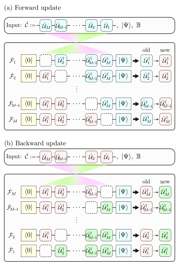
Although we have described the case for updating the unitary operators from $m=1$ to $m=M$, it is apparent that we can reverse the order of updating the unitary operators from $m=M$ to $m=1$, as schematically shown in Fig. 2(b). We shall call the algorithm for updating the unitary operators from $m=1$ to $m=M$ forward update, and the algorithm for updating the unitary operators from $m=M$ to $m=1$ backward update. Furthermore, let us refer to a single set of consecutive updates, forward update followed by backward update, as a sweep.

The most demanding part computationally in the quantum circuit encoding algorithm is to evaluate the fidelity tensor operator $\hat{\mathcal{F}}_{m}$ in Eq. (11). As explained here, this part can be evaluated directly using a quantum computer when the quantum state $|\Psi\rangle$ is given by a linear combination of several quantum circuits as in Eq. (2), which includes the extreme case where $|\Psi\rangle$ is given by a linear combination of direct product states in the computational basis.

Although this procedure can be extended to the case for any number of qubits in principle, here we consider a subsystem composed of two qubits, i.e., $\mathbb{I}_{m}=\{i,j\}$, on which an unitary operator $\hat{\mathcal{U}}_{m}$ acts. Let us introduce the following notation

for the identity and Pauli operators acting on qubit $i$. Then the fidelity tensor operator $\hat{\mathcal{F}}_{m}$ in the two-qubit subsystem $\mathbb{I}_{m}=\{i,j\}$ can be expressed generally as

where $\tilde{f}_{\alpha,\alpha^{\prime}}$ are complex numbers. This is simply because the operator $|n\rangle\langle n^{\prime}|$ in Eq. (13) for all $n,n^{\prime}=0,1,2,3$ can be expanded with a polynomial of the Pauli and identity operators. We thus find that

because

On the other hand, by using the definition of the fidelity tensor operator $\hat{\mathcal{F}}_{m}$ in Eq. (11), we find that

Therefore, $\tilde{f}_{\alpha,\alpha^{\prime}}$ can be determined by estimating the overlap between $\hat{\mathcal{P}}_{i}^{\alpha}\hat{\mathcal{P}}_{j}^{\alpha^{\prime}}|\Psi_{m+1}\rangle$ and $|\Phi_{m-1}\rangle$ for all $\alpha,\alpha^{\prime}=0,1,2,3$. This overlap can be evaluated using a Hadamard test like circuit shown in Fig. 3(a), provided that a quantum circuit $\hat{\Psi}$ generating the quantum state $|\Psi\rangle=\hat{\Psi}|0\rangle$ is already known. However, this is generally not the case but rather the main task of the quantum circuit encoding algorithm is to finding a quantum circuit $\hat{\mathcal{C}}$ that approximately represents $\hat{\Psi}$. Instead, here we assume that $|\Psi\rangle$ is given by a linear combination of quantum circuit states as in Eqs. (2) and (3). In this case, Eq. (43) can be more explicitly written as

where $\hat{f}_{m}^{(\gamma)}$ and $|\psi_{m+1}^{(\gamma)}\rangle$ are defined in Eqs. (22) and (23), respectively. As shown in Fig. 3(b), $f_{\alpha,\alpha^{\prime}}^{(\gamma)}={\rm Tr}_{\mathbb{I}_{m}}[\hat{f}_{m}^{(\gamma)}\hat{\mathcal{P}}_{i}^{\alpha}\hat{\mathcal{P}}_{j}^{\alpha^{\prime}}]$ can now be evaluated separately for each $\gamma$ by using a Hadamard test like circuit on a quantum computer.

Although the quantum circuit encoding algorithm described above in Sec. II.4 can be applied to general cases, there are some exceptions for which care must be taken. For example, when we consider a ground state $|\Psi\rangle$ of a quantum spin system, the state $|\Psi\rangle$ is often in the spin singlet sector. In this case, there is no overlap between $|\Psi\rangle$ and $|0\rangle$ because the product state $|0\rangle$ represents the fully polarized state with the maximum spin value. Therefore, an alternative algorithm is required to construct an initial circuit $\hat{\mathcal{C}}$, for which $\hat{\mathcal{C}}^{\dagger}|\Psi\rangle$ has a finite overlap with $|0\rangle$.

Let us consider the reduced density matrix $\hat{\rho}$ of a quantum state $|\Psi\rangle$ on the subsystem $\mathbb{I}=\{i_{1},i_{2},\mathinner{\cdotp\mkern-2.0mu\cdotp\mkern-2.0mu\cdotp},i_{K}\}$ that is given by

with the associated eigenstates and eigenvalues being denoted as $|\lambda_{n}\rangle$ and $\lambda_{n}$, respectively. Here we assume that $\lambda_{n}$ is in the descending order, i.e., $\lambda_{0}\geq\lambda_{1}\geq\lambda_{2}\geq\mathinner{\cdotp\mkern-2.0mu\cdotp\mkern-2.0mu\cdotp}$. The reduced density matrix $\hat{\rho}$ is then represented as

We shall now find the unitary operator $\hat{\mathcal{V}}_{1}$ in the subsystem $\mathbb{I}$ such that

where $|0\rangle=|0\rangle_{i_{1}}|0\rangle_{i_{2}}\mathinner{\cdotp\mkern-2.0mu\cdotp\mkern-2.0mu\cdotp}|0\rangle_{i_{K}}$ in the computational basis defined in the subsystem $\mathbb{I}$.

For this end, let us first expand $\hat{\mathcal{V}}_{1}$ in the following general form:

where $\{|n\rangle=|\sigma_{i_{1}}\sigma_{i_{2}}\mathinner{\cdotp\mkern-2.0mu\cdotp\mkern-2.0mu\cdotp}\sigma_{i_{K}}\rangle\}_{n=0}^{2^{K}-1}$ are the basis states in the subsystem $\mathbb{I}$. We then find that

It is now easy to find that

yields one of the solutions for Eq. (48). Once we determine the unitary operator $\hat{\mathcal{V}}_{1}$ in Eq. (51), we can assign quantum gates for this operator by following the prescription described in Sec. II.3 for the two-qubit case, if it is required.

In numerical simulations, we can determine $\hat{\mathcal{V}}_{1}$ in Eq. (51) by directly evaluating the eigenstates $|\lambda_{n}\rangle$ of the reduced density operator $\hat{\rho}$. $\hat{\mathcal{V}}_{1}$ can also be determined via a quantum computer. To show this, let us consider the subsystem $\mathbb{I}$ composed of two qubits $\mathbb{I}=\{i,j\}$, for simplicity. Expanding the reduced density matrix $\hat{\rho}$ with a polynomials of the Pauli and identity operators

we find that

This implies that the matrix elements $\tilde{r}_{\alpha,\alpha^{\prime}}$ of $\hat{\rho}$ in Eq. (52) can be determined by measuring all possible pairs of products of the Pauli and identity operators $\hat{\mathcal{P}}_{i}^{\alpha}\hat{\mathcal{P}}_{j}^{\alpha^{\prime}}$ ($\alpha,\alpha^{\prime}=0,1,2,3$). This can be performed on a quantum computer directly if the state $|\Psi\rangle$ is given in a quantum circuit, or by using the procedure described in Sec. II.5 (also see Fig. 3), otherwise. Having estimated the reduced density matrix for $\hat{\rho}$, one can determine the unitary operator $\hat{\mathcal{V}}_{1}$ in Eq. (51) classically. The extension to the subsystem $\mathbb{I}$ composed of more than two qubits is straightforward. We should also note that constructing a reduced density matrix by measuring a set of Pauli and identity operators on a quantum computer is known as quantum state tomography Nielsen and Chuang 2011, and the technique described in Sec. II.5 is also along this line.

This procedure can be easily extended for further adding unitary operators $\hat{\mathcal{V}}_{2},\hat{\mathcal{V}}_{3},\dots$. Let us assume that we have already determined the first unitary operator $\hat{\mathcal{V}}_{1}$ acting on $\mathbb{I}=\{i_{1},i_{2},\mathinner{\cdotp\mkern-2.0mu\cdotp\mkern-2.0mu\cdotp},i_{K}\}$. The location of these qubits is selected among a set of clusters of $K$ qubits $\mathbb{C}=\{\mathbb{I}_{1},\mathbb{I}_{2},\mathinner{\cdotp\mkern-2.0mu\cdotp\mkern-2.0mu\cdotp},\mathbb{I}_{C}\}$ so as to maximize Eq. (48), i.e.,

Let us now define a quantum state $|\tilde{\Psi}_{1}\rangle$ incorporating $\hat{\mathcal{V}}_{1}^{\dagger}$ into the quantum state $|\Psi\rangle$, i.e.,

and consider the reduced density matrix $\hat{\rho}_{1}$ of $|\tilde{\Psi}_{1}\rangle$ on the subsystem $\mathbb{I}^{\prime}=\{i^{\prime}_{1},i^{\prime}_{2},\mathinner{\cdotp\mkern-2.0mu\cdotp\mkern-2.0mu\cdotp},i^{\prime}_{K}\}$ given by

$\hat{\mathcal{V}}_{2}$ is then determined by maximizing $\langle 0|\hat{\mathcal{V}}^{\dagger}_{2}\hat{\rho}_{1}\hat{\mathcal{V}}_{2}|0\rangle$, i.e.,

This procedure can be continued until the desired number $\delta M$ of unitary operators $\hat{\mathcal{V}}_{1},\hat{\mathcal{V}}_{2},\dots,\hat{\mathcal{V}}_{\delta M}$ are added, i.e., $\hat{\mathcal{V}}_{\delta M}^{\dagger}\mathinner{\cdotp\mkern-2.0mu\cdotp\mkern-2.0mu\cdotp}\hat{\mathcal{V}}_{2}^{\dagger}\hat{\mathcal{V}}_{1}^{\dagger}|\Psi\rangle$. Note that the reduced density operators $\hat{\rho}_{1},\hat{\rho}_{2},\dots$ can be evaluated on a quantum computer by the quantum state tomography.

Finally, we combine a prototype algorithm of the quantum circuit encoding described in Sec. II.4 (also see Fig. 2) and the initialization algorithm explained in Sec. II.6, in order to automatically construct an optimal quantum circuit for encoding a give quantum state. Figure 4 summarizes the resulting algorithm that is referred to as automatic quantum circuit encoding (AQCE) algorithm.

The AQCE algorithm is composed of two steps, i.e., the enlargement step in Fig. 4(b) and the optimization step in Fig. 4(c). The inputs of the AQCE algorithm are a target quantum state $|\Psi\rangle$, a quantum circuit $\hat{\mathcal{C}}$ set to be the identity operator $\hat{I}$, and a set of bonds $\mathbb{B}$ of two qubits (or a set of clusters $\mathbb{C}$ of $K$ qubits), as shown in Fig. 4(a). In the first enlargement step, we employ the initialization algorithm as in Fig. 4(b) to construct a quantum circuit $\hat{\mathcal{C}}$ having $M_{0}$ number of unitary operators and finite overlap between $\hat{\mathcal{C}}|0\rangle$ and $|\Psi\rangle$. Then, in the following optimization step, we perform the forward and backward updates of the quantum circuit encoding algorithm to optimize these unitary operators as in Fig. 4(c). The total number of sweeps for the optimization is set to $N$.

Next, we enlarge the quantum circuit by increasing the number $M$ of unitary operators by $\delta M$, i.e., $M=M_{0}+\delta M$, as in Fig. 4(b). This is done one by one by inserting single identity operator next to $|0\rangle$ and perform the backward update of the quantum circuit encoding algorithm to optimize the whole unitary operators. After adding $\delta M$ new unitary operators, we move to the optimization step and perform the forward and backward updates again to optimize each unitary operator as in Fig. 4(c). Notice that expect for the initial enlargement step, we perform in the enlargement step the backward update of the quantum circuit encoding algorithm described in Sec. II.4, which is more efficient than the initialization algorithm described in Sec. II.6. We repeat this whole iteration of the enlargement and optimization steps until the quantum circuit contains the desired number $M_{\rm max}$ of unitary operators. The control parameters in the AQCE algorithm are thus $M_{0}$, $M_{\rm max}$, $\delta M$, and $N$.

Here, we show the numerical demonstration of the quantum circuit encoding for the ground states of the one-dimensional $S=1/2$ isotropic antiferromagnetic Heisenberg model and XY model. The Hamiltonian of these models is given as

where $\hat{X}_{i}$, $\hat{Y}_{i}$, and $\hat{Z}_{i}$ are the $x$-, $y$-, and $z$-components of Pauli operators, respectively, at site $i$ on a one-dimensional chain with $L$ sites under periodic boundary conditions, i.e., $\hat{X}_{L+1}=\hat{X}_{1}$, $\hat{Y}_{L+1}=\hat{Y}_{1}$, and $\hat{Z}_{L+1}=\hat{Z}_{1}$. The Hamiltonian $\hat{\mathcal{H}}$ with $\Delta=1$ and $0$ corresponds to the isotropic Heisenberg and XY models, respectively, and the ground states of these two models are at criticality with algebraically decaying correlation functions.

The ground states $|\Psi\rangle$ of these models are calculated numerically by the standard Lancozs method within the accuracy of the ground state energy $10^{-12}$. Although the AQCE algorithm is formulated deterministically, it turns out that the resulting structure of the quantum circuit depends on the numerical tiny error of the quantum state $|\Psi\rangle$ obtained by finite precision arithmetic. This is simply because even when the fidelity tensor $\hat{\mathcal{F}}_{m}$ for equivalent pairs of qubits is exactly the same theoretically, a particular pair of qubits $\mathbb{I}=\{i,j\}$ may be selected because of the numerical error due to finite precision calculations. Therefore, here we perform 100 AQCE calculations for each system size $L$, in which the ground state $|\Psi\rangle$ is prepared by the Lanczos method with 100 different initial Lanczos vectors, thus implying that the ground state $|\Psi\rangle$ to be encoded is slightly different among these 100 different calculations, and select the best circuit $\hat{\mathcal{C}}$ in terms of the fidelity $|\langle 0|\hat{\mathcal{C}}^{\dagger}|\Psi\rangle|$. In addition, we perform 1000 sweeps to further optimize the unitary operators in the best circuit using the quantum circuit encoding algorithm. The parameters for the AQCE algorithm are $(M_{0},N,\delta M,M_{\rm max})=(L,20,L/2,L(L-5)/2)$ for the XY model and $(M_{0},N,\delta M,M_{\rm max})=(L,20,L/2,L^{2}/2)$ for the isotropic Heisenberg model. We set that $\mathbb{B}$ is composed of all pairs of two sites (i.e., qubits) $\{i,j\}$ with $i,j\in\mathbb{L}$, thus including pairs of distant sites.

References

- Cerezo et al. (2021a) M. Cerezo, Andrew Arrasmith, Ryan Babbush, Simon C. Benjamin, Suguru Endo, Keisuke Fujii, Jarrod R. McClean, Kosuke Mitarai, Xiao Yuan, Lukasz Cincio, and Patrick J. Coles, “Variational quantum algorithms,” Nature Reviews Physics 3, 625–644 (2021a).
- Peruzzo et al. (2014) Alberto Peruzzo, Jarrod McClean, Peter Shadbolt, Man-Hong Yung, Xiao-Qi Zhou, Peter J. Love, Alán Aspuru-Guzik, and Jeremy L. O’Brien, “A variational eigenvalue solver on a photonic quantum processor,” Nature Communications 5, 4213 (2014).
- Yung et al. (2014) M.-H. Yung, J. Casanova, A. Mezzacapo, J. McClean, L. Lamata, A. Aspuru-Guzik, and E. Solano, “From transistor to trapped-ion computers for quantum chemistry,” Scientific Reports 4, 3589 (2014).
- O’Malley et al. (2016) P. J. J. O’Malley, R. Babbush, I. D. Kivlichan, J. Romero, J. R. McClean, R. Barends, J. Kelly, P. Roushan, A. Tranter, N. Ding, B. Campbell, Y. Chen, Z. Chen, B. Chiaro, A. Dunsworth, A. G. Fowler, E. Jeffrey, E. Lucero, A. Megrant, J. Y. Mutus, M. Neeley, C. Neill, C. Quintana, D. Sank, A. Vainsencher, J. Wenner, T. C. White, P. V. Coveney, P. J. Love, H. Neven, A. Aspuru-Guzik, and J. M. Martinis, “Scalable quantum simulation of molecular energies,” Phys. Rev. X 6, 031007 (2016).
- Kandala et al. (2017) Abhinav Kandala, Antonio Mezzacapo, Kristan Temme, Maika Takita, Markus Brink, Jerry M. Chow, and Jay M. Gambetta, “Hardware-efficient variational quantum eigensolver for small molecules and quantum magnets,” Nature 549, 242–246 (2017).
- Shen et al. (2017) Yangchao Shen, Xiang Zhang, Shuaining Zhang, Jing-Ning Zhang, Man-Hong Yung, and Kihwan Kim, “Quantum implementation of the unitary coupled cluster for simulating molecular electronic structure,” Phys. Rev. A 95, 020501(R) (2017).
- Romero et al. (2018) Jonathan Romero, Ryan Babbush, Jarrod R McClean, Cornelius Hempel, Peter J Love, and Alán Aspuru-Guzik, “Strategies for quantum computing molecular energies using the unitary coupled cluster ansatz,” Quantum Science and Technology 4, 014008 (2018).
- Evangelista et al. (2019) Francesco A. Evangelista, Garnet Kin-Lic Chan, and Gustavo E. Scuseria, “Exact parameterization of fermionic wave functions via unitary coupled cluster theory,” The Journal of Chemical Physics 151, 244112 (2019).
- McArdle et al. (2020) Sam McArdle, Suguru Endo, Alán Aspuru-Guzik, Simon C. Benjamin, and Xiao Yuan, “Quantum computational chemistry,” Rev. Mod. Phys. 92, 015003 (2020).
- Schuld et al. (2015) Maria Schuld, Ilya Sinayskiy, and Francesco Petruccione, “An introduction to quantum machine learning,” Contemporary Physics 56, 172–185 (2015).
- Wittek (2014) Peter Wittek, Quantum Machine Learning: What Quantum Computing Means to Data Mining, 1st ed. (Elsevier, San Diego, 2014).
- (12) Jeremy Adcock, Euan Allen, Matthew Day, Stefan Frick, Janna Hinchliff, Mack Johnson, Sam Morley-Short, Sam Pallister, Alasdair Price, and Stasja Stanisic, “Advances in quantum machine learning,” arXiv:1512.02900 [quant-ph] .
- Biamonte et al. (2017) Jacob Biamonte, Peter Wittek, Nicola Pancotti, Patrick Rebentrost, Nathan Wiebe, and Seth Lloyd, “Quantum machine learning,” Nature 549, 195–202 (2017).
- Schuld and Petruccione (2018) Maria Schuld and Francesco Petruccione, Supervised Learning with Quantum Computers, 1st ed. (Springer Publishing Company, Incorporated, 2018).
- Perdomo-Ortiz et al. (2018) Alejandro Perdomo-Ortiz, Marcello Benedetti, John Realpe-Gómez, and Rupak Biswas, “Opportunities and challenges for quantum-assisted machine learning in near-term quantum computers,” Quantum Science and Technology 3, 030502 (2018).
- Mitarai et al. (2018) K. Mitarai, M. Negoro, M. Kitagawa, and K. Fujii, “Quantum circuit learning,” Phys. Rev. A 98, 032309 (2018).
- Amari (1998) Shun-Ichi Amari, “Natural gradient works efficiently in learning,” Neural Comput. 10, 251–276 (1998).
- Seki et al. (2020) Kazuhiro Seki, Tomonori Shirakawa, and Seiji Yunoki, “Symmetry-adapted variational quantum eigensolver,” Phys. Rev. A 101, 052340 (2020).
- Stokes et al. (2020) James Stokes, Josh Izaac, Nathan Killoran, and Giuseppe Carleo, “Quantum Natural Gradient,” Quantum 4, 269 (2020).
- Nakanishi et al. (2020) Ken M. Nakanishi, Keisuke Fujii, and Synge Todo, “Sequential minimal optimization for quantum-classical hybrid algorithms,” Phys. Rev. Research 2, 043158 (2020).
- McClean et al. (2018) Jarrod R. McClean, Sergio Boixo, Vadim N. Smelyanskiy, Ryan Babbush, and Hartmut Neven, “Barren plateaus in quantum neural network training landscapes,” Nature Communications 9, 4812 (2018).
- Cerezo et al. (2021b) M. Cerezo, Akira Sone, Tyler Volkoff, Lukasz Cincio, and Patrick J. Coles, “Cost function dependent barren plateaus in shallow parametrized quantum circuits,” Nature Communications 12, 1791 (2021b).
- Wang et al. (2021) Samson Wang, Enrico Fontana, M. Cerezo, Kunal Sharma, Akira Sone, Lukasz Cincio, and Patrick J. Coles, “Noise-induced barren plateaus in variational quantum algorithms,” Nature Communications 12, 6961 (2021).
- (24) Carlos Ortiz Marrero, Mária Kieferová, and Nathan Wiebe, “Entanglement induced barren plateaus,” arXiv:2010.15968 [quant-ph] .
- Dankert et al. (2009) Christoph Dankert, Richard Cleve, Joseph Emerson, and Etera Livine, “Exact and approximate unitary 2-designs and their application to fidelity estimation,” Phys. Rev. A 80, 012304 (2009).
- Sim et al. (2019) Sukin Sim, Peter D. Johnson, and Alán Aspuru-Guzik, “Expressibility and entangling capability of parameterized quantum circuits for hybrid quantum-classical algorithms,” Advanced Quantum Technologies 2, 1900070 (2019).
- Hubregtsen et al. (2021) Thomas Hubregtsen, Josef Pichlmeier, Patrick Stecher, and Koen Bertels, “Evaluation of parameterized quantum circuits: on the relation between classification accuracy, expressibility, and entangling capability,” Quantum Machine Intelligence 3, 9 (2021).
- Harrow and Low (2009) Aram W. Harrow and Richard A. Low, “Random quantum circuits are approximate 2-designs,” Communications in Mathematical Physics 291, 257–302 (2009).
- Diniz and Jonathan (2011) Igor Tuche Diniz and Daniel Jonathan, “Comment on “random quantum circuits are approximate 2-designs” by a.w. harrow and r.a. low (commun. math. phys. 291, 257–302 (2009)),” Communications in Mathematical Physics 304, 281–293 (2011).
- (30) Zoë Holmes, Kunal Sharma, M. Cerezo, and Patrick J. Coles, “Connecting ansatz expressibility to gradient magnitudes and barren plateaus,” arXiv:2101.02138 [quant-ph] .
- (31) Kosuke Mitarai, Yasunari Suzuki, Wataru Mizukami, Yuya O. Nakagawa, and Keisuke Fujii, “Quadratic clifford expansion for efficient benchmarking and initialization of variational quantum algorithms,” arXiv:2011.09927 [quant-ph] .
- Vidal (2007) G. Vidal, “Entanglement renormalization,” Phys. Rev. Lett. 99, 220405 (2007).
- Vidal (2008) G. Vidal, “Class of quantum many-body states that can be efficiently simulated,” Phys. Rev. Lett. 101, 110501 (2008).
- Evenbly and Vidal (2009) G. Evenbly and G. Vidal, “Algorithms for entanglement renormalization,” Phys. Rev. B 79, 144108 (2009).
- Cong et al. (2019) Iris Cong, Soonwon Choi, and Mikhail D. Lukin, “Quantum convolutional neural networks,” Nature Physics 15, 1273–1278 (2019).
- Pesah et al. (2021) Arthur Pesah, M. Cerezo, Samson Wang, Tyler Volkoff, Andrew T. Sornborger, and Patrick J. Coles, “Absence of barren plateaus in quantum convolutional neural networks,” Phys. Rev. X 11, 041011 (2021).
- Grimsley et al. (2019) Harper R. Grimsley, Sophia E. Economou, Edwin Barnes, and Nicholas J. Mayhall, “An adaptive variational algorithm for exact molecular simulations on a quantum computer,” Nature Communications 10, 3007 (2019).
- Tang et al. (2021) Ho Lun Tang, V.O. Shkolnikov, George S. Barron, Harper R. Grimsley, Nicholas J. Mayhall, Edwin Barnes, and Sophia E. Economou, “Qubit-adapt-vqe: An adaptive algorithm for constructing hardware-efficient ansätze on a quantum processor,” PRX Quantum 2, 020310 (2021).
- Liu et al. (2021) Jie Liu, Zhenyu Li, and Jinlong Yang, “An efficient adaptive variational quantum solver of the schrödinger equation based on reduced density matrices,” The Journal of Chemical Physics 154, 244112 (2021).
- Yao et al. (2021) Yong-Xin Yao, Niladri Gomes, Feng Zhang, Cai-Zhuang Wang, Kai-Ming Ho, Thomas Iadecola, and Peter P. Orth, “Adaptive variational quantum dynamics simulations,” PRX Quantum 2, 030307 (2021).
- Zhang et al. (2021) Feng Zhang, Niladri Gomes, Yongxin Yao, Peter P. Orth, and Thomas Iadecola, “Adaptive variational quantum eigensolvers for highly excited states,” Phys. Rev. B 104, 075159 (2021).
- Trotter (1959) H. F. Trotter, “On the product of semi-groups of operators,” Proceedings of the American Mathematical Society 10, 545–551 (1959).
- Suzuki (1976) Masuo Suzuki, “Relationship between d-Dimensional Quantal Spin Systems and (d+1)-Dimensional Ising Systems: Equivalence, Critical Exponents and Systematic Approximants of the Partition Function and Spin Correlations,” Progress of Theoretical Physics 56, 1454–1469 (1976).
- Lloyd (1996) Seth Lloyd, “Universal quantum simulators,” Science 273, 1073–1078 (1996).
- (45) IBM, “Ibm quantum,” https://quantum-computing.ibm.com.
- (46) M. Cerezo, Kunal Sharma, Andrew Arrasmith, and Patrick J. Coles, “Variational quantum state eigensolver,” arXiv:2004.01372 [quant-ph] .
- (47) Apart from a global phase factor that is irrelevant to the discussion here.
- Nielsen and Chuang (2011) Michael A. Nielsen and Isaac L. Chuang, Quantum Computation and Quantum Information: 10th Anniversary Edition, 10th ed. (Cambridge University Press, USA, 2011).
- Kraus and Cirac (2001) B. Kraus and J. I. Cirac, “Optimal creation of entanglement using a two-qubit gate,” Phys. Rev. A 63, 062309 (2001).
- Vidal and Dawson (2004) G. Vidal and C. M. Dawson, “Universal quantum circuit for two-qubit transformations with three controlled-not gates,” Phys. Rev. A 69, 010301 (2004).
- Coffey et al. (2008) Mark W. Coffey, Ron Deiotte, and Torey Semi, “Comment on “universal quantum circuit for two-qubit transformations with three controlled-not gates” and “recognizing small-circuit structure in two-qubit operators”,” Phys. Rev. A 77, 066301 (2008).
- Vatan and Williams (2004) Farrokh Vatan and Colin Williams, “Optimal quantum circuits for general two-qubit gates,” Phys. Rev. A 69, 032315 (2004).
- Schuld and Petruccione (2019) Maria Schuld and Francesco Petruccione, Supervised Learning with Quantum Computers (Springer, Switzerland, 2019).
- Shirakawa et al. (2021) Tomonori Shirakawa, Kazuhiro Seki, and Seiji Yunoki, “Discretized quantum adiabatic process for free fermions and comparison with the imaginary-time evolution,” Phys. Rev. Research 3, 013004 (2021).
- Barends et al. (2015) R. Barends, L. Lamata, J. Kelly, L. García-Álvarez, A. G. Fowler, A. Megrant, E. Jeffrey, T. C. White, D. Sank, J. Y. Mutus, B. Campbell, Yu Chen, Z. Chen, B. Chiaro, A. Dunsworth, I.-C. Hoi, C. Neill, P. J. J. O’Malley, C. Quintana, P. Roushan, A. Vainsencher, J. Wenner, E. Solano, and John M. Martinis, “Digital quantum simulation of fermionic models with a superconducting circuit,” Nature Communications 6, 7654 (2015).
- Barends et al. (2016) R. Barends, A. Shabani, L. Lamata, J. Kelly, A. Mezzacapo, U. Las Heras, R. Babbush, A. G. Fowler, B. Campbell, Yu Chen, Z. Chen, B. Chiaro, A. Dunsworth, E. Jeffrey, E. Lucero, A. Megrant, J. Y. Mutus, M. Neeley, C. Neill, P. J. J. O’Malley, C. Quintana, P. Roushan, D. Sank, A. Vainsencher, J. Wenner, T. C. White, E. Solano, H. Neven, and John M. Martinis, “Digitized adiabatic quantum computing with a superconducting circuit,” Nature 534, 222–226 (2016).
- Evenbly and Vidal (2011) G. Evenbly and G. Vidal, “Tensor network states and geometry,” Journal of Statistical Physics 145, 891–918 (2011).
- Schuld et al. (2016) Maria Schuld, Ilya Sinayskiy, and Francesco Petruccione, “Prediction by linear regression on a quantum computer,” Phys. Rev. A 94, 022342 (2016).
- Grover (2000) Lov K. Grover, “Synthesis of quantum superpositions by quantum computation,” Phys. Rev. Lett. 85, 1334–1337 (2000).
- Shende et al. (2006) V.V. Shende, S.S. Bullock, and I.L. Markov, “Synthesis of quantum-logic circuits,” IEEE Transactions on Computer-Aided Design of Integrated Circuits and Systems 25, 1000–1010 (2006).
- Plesch and Brukner (2011) Martin Plesch and Časlav Brukner, “Quantum-state preparation with universal gate decompositions,” Phys. Rev. A 83, 032302 (2011).
- Sanders et al. (2019) Yuval R. Sanders, Guang Hao Low, Artur Scherer, and Dominic W. Berry, “Black-box quantum state preparation without arithmetic,” Phys. Rev. Lett. 122, 020502 (2019).
- (63) Kouhei Nakaji, Shumpei Uno, Yohichi Suzuki, Rudy Raymond, Tamiya Onodera, Tomoki Tanaka, Hiroyuki Tezuka, Naoki Mitsuda, and Naoki Yamamoto, “Approximate amplitude encoding in shallow parameterized quantum circuits and its application to financial market indicator,” arXiv:2103.13211 [quant-ph] .
- (64) Standard test images available in ImageProcessingPlace.com.
- (65) E. Miles Stoudenmire and David J. Schwab, “Supervised Learning with Quantum-Inspired Tensor Networks,” arXiv:1605.05775 [stat.ML] .
- Mezzadri (2007) Francesco Mezzadri, “How to generate random matrices from the classical compact groups,” NOTICE of the AMS 54, 592 (2007).
- (67) In practice, we can obtain, for example, and by performing the SVD of the matrix , where is defined as .