跳到论文正文
W Papers独立论文阅读器 arXiv:2112.14451 论文正文 计算阅读时间 · 0%
引用这篇论文根据当前论文元数据生成,正式投稿前建议核对。


License: arXiv.org perpetual non-exclusive license
arXiv:2112.14451v1 [q-fin.RM] 29 Dec 2021

Dynamic growth-optimum portfolio choice
under risk control

Pengyu Wei Thanks: Division of Banking and Finance, Nanyang Business School, Nanyang Technological University, Singapore. E-mail: pengyu.wei@ntu.edu.sg.    Zuo Quan Xu Thanks: Department of Applied Mathematics, The Hong Kong Polytechnic University, Hong Kong. Email: maxu@polyu.edu.hk.
August 11, 2026
Abstract

This paper studies a mean-risk portfolio choice problem for log-returns in a continuous-time, complete market. This is a growth-optimal problem with risk control. The risk of log-returns is measured by weighted Value-at-Risk (WVaR), which is a generalization of Value-at-Risk (VaR) and Expected Shortfall (ES). We characterize the optimal terminal wealth up to the concave envelope of a certain function, and obtain analytical expressions for the optimal wealth and portfolio policy when the risk is measured by VaR or ES. In addition, we find that the efficient frontier is a concave curve that connects the minimum-risk portfolio with the growth optimal portfolio, as opposed to the vertical line when WVaR is used on terminal wealth. Our results advocate the use of mean-WVaR criterion for log-returns instead of terminal wealth in dynamic portfolio choice.

Keywords: Mean-risk portfolio choice; growth-optimum; log-return; weighted Value-at-Risk; efficient frontier; quantile formulation

1 Introduction

The growth-optimal portfolio (GOP) is a portfolio which has a maximal expected growth rate (namely log-return) over any time horizon. As the GOP can be usually tracked to the work Kelly, 1956, it is also called the “Kelly criterion”. The GOP can also be obtained by maximizing log-utility which has a longer history. As the name implies, it can be used to maximize the expected growth rate of a portfolio. Indeed, it performs in some sense better than any other significantly different strategy as the time horizon increases.

Over the past half century, a lot of papers have investigated the GOP. In theory and practice, the GOP has widely applications in a large number of areas including portfolio theory, utility theory, game theory, information theory, asset pricing theory, insurance theory. For instance, to name a few of them in the recent studies in the literature, Aurell et al., 2000 study asset pricing problems in incomplete market; Rotar, 2004 considers optimal investment problems; Thorp, 2000 applies it to casino games.

We want to emphasize that the GOP ignores the relevant risk when maximizing the expected growth rate of a portfolio. It is the seminal work Markowitz, 1952 that takes the trade-off between the portfolio return and its risk into consideration when an investor chooses a portfolio. Markowitz, 1952 suggests to use variance to measure the risk. Since then, the mean-variance theory becomes one of the most dominant financial theories in the realm of portfolio choice. Besides variance, alternative risk measures have been proposed to measure the risk for portfolio choice. Research along this line includes Rockafellar and Uryasev, 2000, Campbell et al., 2001, Rockafellar and Uryasev, 2002, Alexander and Baptista, 2002, Alexander and Baptista, 2004, Jin et al., 2006, and Adam et al., 2008, where the authors study single-period mean-risk portfolio selection with various risk measures, such as semi-variance, value-at-risk (VaR), expected shortfall (ES), and spectral risk measures.

There also have numerous extensions of the mean-risk portfolio optimization from the single-period setting to the dynamic, continuous-time one (Zhou and Li, 2000; Bielecki et al., 2005; Jin et al., 2005; Basak and Chabakauri, 2010; He et al., 2015; Zhou et al., 2017; Gao et al., 2017; Dai et al., 2021; He and Jiang, 2021, e.g.). In particular, He et al., 2015 study a continuous-time mean-risk portfolio choice when risk is measured by the weighted Value-at-Risk (WVaR) but their results are rather pessimistic. The WVaR is a quantile-based risk measure that generalizes VaR and ES, two popular risk measures in quantitative risk management. They find that, when using WVaR (including VaR and ES) on terminal wealth to measure portfolio risk, the mean-risk model is prone to be ill-posed (i.e., the optimal value is infinite) and the investor tends to take infinite leverage on risky assets, leading to extremely risk-taking behaviors. Furthermore, the optimal risk is independent of the expected terminal target so the efficient frontier is a vertical line on the mean-WVaR plane. Their results suggest that the mean-WVaR model is an improper modeling of the trade-off between return and risk, when the WVaR is applied to the terminal wealth.

This paper proposes a continuous-time portfolio choice model with mean-WVaR criterion for portfolio log-returns, as opposed to the mean-WVaR criterion for terminal wealth in He et al., 2015. The motivation is two-fold. First, the mean-risk criterion for log-returns is consistent with Markowitz’s original idea to use mean and variance on portfolio returns. We consider a growth-optimal problem with risk control. Moreover, many single-period mean-risk models use risk measures on portfolio returns in the literature (Alexander and Baptista, 2002; Alexander and Baptista, 2004; Alexander and Baptista, 2006; Jin et al., 2006; Adam et al., 2008, e.g.). However, there is a discrepancy between single-period and dynamic portfolio choice models, as the latter typically considers mean-risk criterion for terminal wealth; an exception is Dai et al., 2021 who study continuous-time mean-variance portfolio choice for portfolio log-returns. We similarly adopt the mean-WVaR criterion for log-returns which naturally generalize the single-period return when returns are continuously compounded. Second, such a criterion conquers the ill-posedness of the model in He et al., 2015. As noted in He et al., 2015, the mean-WVaR criterion for terminal wealth is essentially a linear program for the quantile function of terminal wealth. This linearity, in turn, leads to the optimal terminal wealth’s quantile function being “corner points”, leading to extreme risk-taking behaviors. By contrast, our mean-WVaR criterion for log-returns is not linear in the quantile function of terminal wealth, and thus conquers the ill-posedness.

In a continuous-time, complete market framework, we solve the mean-WVaR portfolio choice for log-returns with the help of the so-called quantile formulation, developed in a series of papers (Schied, 2004; Carlier and Dana, 2006; Jin and Zhou, 2008; He and Zhou, 2011; Carlier and Dana, 2011; Xia and Zhou, 2016; Xu, 2016, e.g.). When risk is measured by a general WVaR risk measure, we characterize the optimal terminal wealth up to the concave envelope of a certain function through a detailed and involved analysis. When risk is measured by VaR or ES, two special cases of WVaR, we derive analytical expressions for the optimal terminal wealth and portfolio policy. The optimal terminal wealth turns out to be closely related to the growth optimal portfolio: the investor classifies market scenarios into different states, in which the terminal payoff can be constant, a multiple or fraction of the growth optimal portfolio. Furthermore, we obtain the efficient frontier, which is a concave curve that connects the minimum-risk (min-risk) portfolio with the growth optimal portfolio, as opposed to the vertical line in He et al., 2015. Our model allows for a meaningful characterization of the risk-return trade-off and may serve as a guideline for investors to set a reasonable investment target. Although He et al., 2015 provides a critique of using WVaR to measure risk, our results advocate that it is more appropriate to use WVaR, in particular, VaR and ES, on portfolio log-returns instead of terminal wealth for dynamic portfolio choice.

The rest of the paper is organized as follows. In Section 2, we propose a mean-WVaR portfolio choice problem for portfolio log-returns. We solve the problem in Section 3 by quantile optimization method. Section 4 presents optimal solutions and efficient frontiers when the risk is measured by VaR or ES. Some new financial insights and a comparation to the existing work are presented as well. Some concluding remarks are given in Section 5. Appendix A contains three useful lemmas. All remaining proofs are placed in Appendix B.

2 Mean-WVaR portfolio choice model

2.1 Financial market

Let T>0T>0 be a given terminal time and (Ω,ℱ,{ℱt}0≤t≤T,ℙ)(\Omega,\mathcal{F},\{\mathcal{F}_{t}\}_{0\leq t\leq T},\mathbb{P}) be a filtered probability space, on which is defined a standard one-dimensional Brownian motion {Wt}0≤t≤T\{W_{t}\}_{0\leq t\leq T}. It is assumed that ℱt=σ{Ws,0≤s≤t}\mathcal{F}_{t}=\sigma\{W_{s},0\leq s\leq t\} augmented by all ℙ\mathbb{P}-null sets and that ℱ=ℱT\mathcal{F}=\mathcal{F}_{T} is ℙ\mathbb{P} complete.

We consider a Black-Scholes market in which there are a risk-free asset and a risky asset (called stock). The risk-free asset pays a constant interest rate r>0r>0 and the stock price SS follows a geometric Brownian motion

d​StSt=μ​d​t+σ​d​Wt,\frac{dS_{t}}{S_{t}}=\mu dt+\sigma dW_{t},

where μ\mu and σ\sigma, the appreciation rate and volatility of the stock, are positive constants. There exists a unique positive state price density (pricing kernel) process ξ\xi11 1 With additional assumptions on ξT\xi_{T}, our main results can be extended to a general complete market with stochastic investment opportunities. satisfying

d​ξtξt=−r​d​t−θ​d​Wt,ξ0=1,\frac{d\xi_{t}}{\xi_{t}}=-rdt-\theta dW_{t},\quad\xi_{0}=1, (2.1)

where θ=(μ−r)/σ\theta=(\mu-r)/\sigma is the market price of risk in the economy. Therefore the market is complete.

Consider an economic agent with an initial endowment x>0x>0 and faced an investment time horizon [0,T][0,T]. The agent chooses a dynamic investment strategy πt\pi_{t}, which represents the dollar amount invested in the stock at time tt. Assume the trading is continuous in a self-financing fashion and there are no transaction costs. The agent’s wealth process XtX_{t} then follows a stochastic differential equation

d​Xt=[r​Xt+(μ−r)​πt]​d​t+σ​πt​d​Wt,X0=x.dX_{t}=\left[rX_{t}+(\mu-r)\pi_{t}\right]dt+\sigma\pi_{t}dW_{t},~X_{0}=x. (2.2)

The portfolio process πt\pi_{t} is called an admissible portfolio if it is {ℱt}0≤t≤T\{\mathcal{F}_{t}\}_{0\leq t\leq T} progressively measurable with ∫0Tπt2​𝑑t<∞,a.s.\int_{0}^{T}\pi_{t}^{2}dt<\infty,a.s., and the corresponding terminal wealth satisfies XT≥0,a.sX_{T}\geq 0,a.s.

Let RTR_{T} be the continuously compounded return (log-return) over the horizon [0,T][0,T], i.e.,

RT=1T​ln⁡XTx.R_{T}=\frac{1}{T}\ln\frac{X_{T}}{x}. (2.3)

By convention, we define

ln⁡0=lims↓0ln⁡s=−∞​ and ​e−∞=lims↓−∞es=0.\ln 0=\lim_{s\downarrow 0}\ln s=-\infty\mbox{ and }e^{-\infty}=\lim_{s\downarrow-\infty}e^{s}=0.

2.2 Risk measure

We now introduce a risk measure that will be used in the portfolio choice model. In this paper, we focus on the weighted VaR (WVaR) risk measure proposed by He et al., 2015, which is a generalization of Value-at-Risk (VaR) and Expected Shortfall (ES), and encompasses many well-known risk measures that are widely used in finance and actuarial sciences, such as spectral risk measures and distortion risk measures; see Wei, 2018 for a review.

For any ℱT\mathcal{F}_{T}-measurable random variable XX, let FXF_{X} denote its cumulative distribution function; and let GXG_{X} denote its quantile function defined by

GX​(z)=inf{x∈ℝ:FX​(x)>z}=sup{x∈ℝ:FX​(x)≤z},z∈[0,1),G_{X}(z)=\inf\{x\in\mathbb{R}:F_{X}(x)>z\}=\sup\{x\in\mathbb{R}:F_{X}(x)\leq z\},~z\in[0,1),

with the convention GX​(1)=limz↑1GX​(z)G_{X}(1)=\lim_{z\uparrow 1}G_{X}(z). The quantile function GXG_{X} is non-decreasing, right-continuous with left limits (RCLL).

The WVaR risk measure for XX is defined as

ρΦ(X)=−∫[0,1]GX(z)Φ(dz),\rho_{\Phi}(X)=-\int_{[0,1]}G_{X}(z)\Phi(dz), (2.4)

where Φ∈P⁡[0,1]\Phi\in P[0,1] and P⁡[0,1]P[0,1] is the set of all probability measures on [0,1][0,1].

The WVaR is a law-invariant comonotonic additive risk measure, and it covers many law-invariant coherent risk measures; see He et al., 2015 for a more detailed discussion. If Φ\Phi is the Dirac measure at α\alpha, i.e., Φ⁡(A)=𝟏α∈A\Phi(A)=\mathbf{1}_{\alpha\in A}, for all A⊂[0,1]A\subset[0,1], then the corresponding WVaR measure becomes the VaR at α\alpha, in other words,

ρΦ​(X)=VaRα​(X)=−GX​(α).\rho_{\Phi}(X)=\text{VaR}_{\alpha}(X)=-G_{X}(\alpha).

If Φ\Phi admits a density ϕ⁡(z)=1α​𝟏z≤α,∀z∈[0,1]\phi(z)=\frac{1}{\alpha}\mathbf{1}_{z\leq\alpha},~\forall z\in[0,1], then the corresponding WVaR measure becomes the ES, i.e.,

ρΦ(X)=ESα(X)=−1α∫0αGX(z)dz.\rho_{\Phi}(X)=\text{ES}_{\alpha}(X)=-\frac{1}{\alpha}\int_{0}^{\alpha}G_{X}(z)dz.

In the original paper of He et al., 2015, WVaR is applied to measure the risk of a portfolio’s terminal wealth. In this paper, we propose to apply WVaR to the portfolio’s log-return instead of its terminal wealth. Let XTX_{T} be the terminal wealth of a portfolio and RTR_{T} be the log-return of XTX_{T}. Due to the monotonicity of logarithm functions, the quantile function of RTR_{T} is

GRT​(z)=1T​ln⁡GXT​(z)x,z∈[0,1].G_{R_{T}}(z)=\frac{1}{T}\ln\frac{G_{X_{T}}(z)}{x},~z\in[0,1].

Therefore, the WVaR of RTR_{T} can be expressed as

ρΦ(RT)=−∫[0,1]1TlnGXT​(z)xΦ(dz)=−1T∫[0,1]lnGXT(z)Φ(dz)+1Tlnx.\rho_{\Phi}(R_{T})=-\int_{[0,1]}\frac{1}{T}\ln\frac{G_{X_{T}}(z)}{x}\Phi(dz)=-\frac{1}{T}\int_{[0,1]}\ln G_{X_{T}}(z)\Phi(dz)+\frac{1}{T}\ln x. (2.5)

However, the extension from terminal wealth to log-return is not straightforward as the integral in (2.5) may not be well-defined since XTX_{T} may take the value of 0 with positive probability. Let

𝔾={G(⋅):[0,1]→[0,+∞],\displaystyle\mathbb{G}=\Big\{G(\cdot)\colon[0,1]\to[0,+\infty], G​ is nondecreasing and RCLL on [0,1],\displaystyle G\text{ is nondecreasing and RCLL on [0,1], }
left-continuous at 1, and finite-valued on [0,1)}\displaystyle\text{ left-continuous at }1,\text{ and finite-valued on }[0,1)\Big\}

be the set of quantile functions of all non-negative random variables, which include all terminal wealth of admissible portfolios. For any G∈𝔾G\in\mathbb{G} and Φ∈P⁡[0,1]\Phi\in P[0,1], the integral ∫[0,1]ln⁡G⁡(z)​Φ​(𝑑z)\int_{[0,1]}\ln G(z)\Phi(dz) is not well-defined if G⁡(s)=0G(s)=0 for some s∈[0,1]s\in[0,1] such that Φ⁡([0,s])>0\Phi([0,s])>0. Define

𝔾Φ={G∈𝔾:G(s)>0 if Φ([0,s])>0,∀s∈[0,1]}.\mathbb{G}_{\Phi}=\big\{G\in\mathbb{G}\colon G(s)>0\text{ if }\Phi([0,s])>0,~\forall s\in[0,1]\big\}.

We set

∫[0,1]ln⁡G⁡(z)​Φ​(𝑑z)=−∞,∀G∈𝔾∖𝔾Φ.\int_{[0,1]}\ln G(z)\Phi(dz)=-\infty,~\forall G\in\mathbb{G}\setminus\mathbb{G}_{\Phi}. (2.6)

Intuitively, if the terminal wealth of a portfolio is 00 (so that the log-return is −∞-\infty) in some states, and the weighting measure Φ\Phi assigns non-zero weighs to these states, then the WVaR of the log-return is assumed to be −∞-\infty. In particular, 𝔼⁡[RT]=−∞{\mathbb{E}}[R_{T}]=-\infty if ℙ⁡(XT=0)>0\mathbb{P}(X_{T}=0)>0.22 2 It is straightforward to verify 𝔼⁡[max⁡(RT,0)]<∞{\mathbb{E}}\left[\max\left(R_{T},0\right)\right]<\infty, given that ξT\xi_{T} is log-normally distributed.

2.3 Portfolio choice model

We assume the agent chooses a dynamic portfolio strategy in the period [0,T][0,T] to maximize the expected log-return while minimizing the risk of the portfolio’s log-return. The risk is evaluated by a WVaR risk measure ρΦ\rho_{\Phi} on the portfolio’s log-return RTR_{T}. Specifically, we consider the following dynamic portfolio choice problem

maxπt\displaystyle\max_{\pi_{t}} λ​𝔼​[RT]−ρΦ​(RT)\displaystyle\lambda{\mathbb{E}}[R_{T}]-\rho_{\Phi}(R_{T}) (2.7)
subject to\displaystyle\text{subject to} dXt=[rXt+(μ−r)πt]dt+σπtdWt,XT≥0,X0=x,\displaystyle dX_{t}=\left[rX_{t}+(\mu-r)\pi_{t}\right]dt+\sigma\pi_{t}dW_{t},~X_{T}\geq 0,~X_{0}=x,
RT=1T​ln⁡XTx,\displaystyle R_{T}=\frac{1}{T}\ln\frac{X_{T}}{x},

where λ≥0\lambda\geq 0 is a “risk-tolerance” parameter that reflects the investor’s tradeoff between return and risk. This is a stochastic control problem, but not standard (namely, unlike those in Yong and Zhou, 1999) due to the existence of the nonlinear probability measure Φ\Phi.

In view of the standard martingale method, e.g., Karatzas and Shreve, 1998, we can first solve the following static optimization problem33 3 This formulation implies that the optimal log-return RTR_{T} is independent of xx.

maxXT∈ℱT\displaystyle\max_{X_{T}\in\mathcal{F}_{T}} λ​𝔼​[RT]−ρΦ​(RT)\displaystyle\lambda{\mathbb{E}}[R_{T}]-\rho_{\Phi}(R_{T}) (2.8)
subject to\displaystyle\text{subject to} 𝔼[ξTXT]≤x,XT≥0,\displaystyle{\displaystyle\mathbb{E}}[\xi_{T}X_{T}]\leq x,~X_{T}\geq 0,
RT=1T​ln⁡XTx,\displaystyle R_{T}=\frac{1}{T}\ln\frac{X_{T}}{x},

where ξT\xi_{T} is given by (2.1). Then apply backward stochastic control theory to derive the corresponding optimal portfolio strategy πt\pi_{t}.

The optimization problem (2.8) nests two special cases.

Case λ=0\lambda=0.

In this case the investor minimizes the risk without any consideration of the expected log-return, and solves the following minimum-risk problem

minXT∈ℱT\displaystyle\min_{X_{T}\in\mathcal{F}_{T}} ρΦ​(RT)\displaystyle\rho_{\Phi}(R_{T}) (2.9)
subject to\displaystyle\text{subject to} 𝔼[ξTXT]≤x,XT≥0,\displaystyle{\displaystyle\mathbb{E}}[\xi_{T}X_{T}]\leq x,~X_{T}\geq 0,
RT=1T​ln⁡XTx.\displaystyle R_{T}=\frac{1}{T}\ln\frac{X_{T}}{x}.

The resulting portfolio is termed the min-risk portfolio.

Case λ=∞\lambda=\infty.

In this case the investor maximizes the expected log-return without any consideration of the risk. This is the so-called growth-optimal problem

maxXT∈ℱT\displaystyle\max_{X_{T}\in\mathcal{F}_{T}} 𝔼⁡[RT]\displaystyle{\displaystyle\mathbb{E}}[R_{T}] (2.10)
subject to\displaystyle\text{subject to} 𝔼[ξTXT]≤x,XT≥0,\displaystyle{\displaystyle\mathbb{E}}[\xi_{T}X_{T}]\leq x,~X_{T}\geq 0,
RT=1T​ln⁡XTx.\displaystyle R_{T}=\frac{1}{T}\ln\frac{X_{T}}{x}.

The optimal solution to (2.10) is well-known in the literature, i.e., the growth-optimal portfolio (or Kelly, 1956 strategy) given by

XKelly=xξT.X_{\textrm{Kelly}}=\frac{x}{\xi_{T}}. (2.11)

The corresponding log-return is

RKelly=1T​ln⁡XKellyx=−1T​ln⁡ξT,R_{\textrm{Kelly}}=\frac{1}{T}\ln\frac{X_{\textrm{Kelly}}}{x}=-\frac{1}{T}\ln\xi_{T},

and its expected value is

𝔼⁡[RKelly]=−1T​𝔼​[ln⁡ξT]=r+θ22.{\mathbb{E}}[R_{\textrm{Kelly}}]=-\frac{1}{T}{\mathbb{E}}[\ln\xi_{T}]=r+\frac{\theta^{2}}{2}.

3 Quantile formulation and optimal solution

In this section, we solve the optimization problem (2.8) for 0≤λ<∞0\leq\lambda<\infty.

If Φ⁡({1})>0\Phi(\{1\})>0, then ρΦ​(RT)=−∞\rho_{\Phi}(R_{T})=-\infty. If Φ\Phi is the the uniform measure on [0,1][0,1], then ρΦ​(RT)=−𝔼⁡[RT]\rho_{\Phi}(R_{T})=-{\mathbb{E}}[R_{T}] and the growth optimal portfolio (2.11) is optimal to (2.8). To exclude these trivial cases, we make the following assumption on Φ\Phi from now on.

Assumption 3.1.

Φ⁡({1})=0\Phi(\{1\})=0 and Φ\Phi is not the uniform measure on [0,1][0,1].

The objective in (2.8) is based on the quantile function of the log-return; thus, the standard convex duality method is not readily applicable. To overcome this difficulty, we employ the quantile formulation, developed in a series of papers including Schied, 2004, Carlier and Dana, 2006, Jin and Zhou, 2008, He and Zhou, 2011, Carlier and Dana, 2011, Xia and Zhou, 2016, and Xu, 2016, to change the decision variable in (2.8) from the terminal wealth XTX_{T} to its quantile function. This allows us to recover the hidden convexity of the problem and solve it completely.

We first show that the budget constraint in (2.8) must hold with equality and the objective function is improved with a higher level of initial wealth.

Lemma 3.1.

If XT∗X_{T}^{*} is an optimal solution to the problem (2.8), then 𝔼⁡[ξT​XT∗]=x{\mathbb{E}}[\xi_{T}X_{T}^{*}]=x.

All the proofs of our results are put in Appendix B.

Denote by FξF_{\xi} and GξG_{\xi} the distribution and quantile functions of ξT\xi_{T}, respectively. With slight abuse of notation, we suppress the subscript TT when there is no need to emphasize the dependence on TT. Since ξT\xi_{T} is log-normally distributed, both FξF_{\xi} and GξG_{\xi} are C∞C^{\infty} functions. The following lemma can be found in Jin and Zhou, 2008.

Lemma 3.2 (Jin and Zhou, 2008).

We have 𝔼⁡[ξT​GX​(1−Fξ​(ξT))]≤𝔼⁡[ξT​XT]{\mathbb{E}}\left[\xi_{T}G_{X}\left(1-F_{\xi}(\xi_{T})\right)\right]\leq{\mathbb{E}}[\xi_{T}X_{T}] for any lower bounded random variable XTX_{T} whose quantile function is GXG_{X}. Furthermore, if 𝔼⁡[ξT​GX​(1−Fξ​(ξT))]<∞{\mathbb{E}}[\xi_{T}G_{X}(1-F_{\xi}(\xi_{T}))]<\infty, then the inequality becomes equality if and only if XT=GX​(1−Fξ​(ξT)),a.s.X_{T}=G_{X}\left(1-F_{\xi}(\xi_{T})\right),~a.s.

From Lemmas 3.1 and 3.2, we know that if XTX_{T} is optimal to (2.8), then XT=GX​(1−Fξ​(ξT))X_{T}=G_{X}(1-F_{\xi}(\xi_{T})) where GXG_{X} is the quantile function of XTX_{T}. Let RTR_{T} be the log-return of XTX_{T}. We have

𝔼⁡[RT]=∫[0,1)1T​ln⁡GX​(z)x​𝑑z,{\mathbb{E}}[R_{T}]=\int_{[0,1)}\frac{1}{T}\ln\frac{G_{X}(z)}{x}dz,
ρΦ(RT)=−∫[0,1)1TlnGX​(z)xΦ(dz),\rho_{\Phi}(R_{T})=-\int_{[0,1)}\frac{1}{T}\ln\frac{G_{X}(z)}{x}\Phi(dz),

and

𝔼⁡[ξT​XT]=∫[0,1)GX​(z)​Gξ​(1−z)​𝑑z.{\mathbb{E}}[\xi_{T}X_{T}]=\int_{[0,1)}G_{X}(z)G_{\xi}(1-z)dz.

Therefore, we can consider the following quantile formulation of (2.8)

maxG∈𝔾\displaystyle\max_{G\in\mathbb{G}} λ​∫[0,1)1T​ln⁡G⁡(z)x​dz+∫[0,1)1T​ln⁡G⁡(z)x​Φ​(dz)\displaystyle\lambda\int_{[0,1)}\frac{1}{T}\ln\frac{G(z)}{x}dz+\int_{[0,1)}\frac{1}{T}\ln\frac{G(z)}{x}\Phi(dz) (3.1)
subject to\displaystyle\text{subject to} ∫[0,1)G⁡(z)​Gξ​(1−z)​dz=x,\displaystyle\int_{[0,1)}G(z)G_{\xi}(1-z)dz=x,

where the decision variable GG is the quantile function of the terminal wealth. Once we obtain the optimal solution G∗G^{*} to (3.1), then the optimal solution to (2.8) is given by

XT∗=G∗​(1−Fξ​(ξT)).X_{T}^{*}=G^{*}\left(1-F_{\xi}(\xi_{T})\right).

Define

w⁡(s)=∫[0,s)Gξ​(1−z)​𝑑z𝔼⁡[ξT],s∈[0,1].w(s)=\frac{\int_{[0,s)}G_{\xi}(1-z)dz}{{\mathbb{E}}[\xi_{T}]},~s\in[0,1]. (3.2)

Because ξT\xi_{T} is log-normally distributed, ww is a C∞C^{\infty} function with w⁡(0)=0w(0)=0, w⁡(1)=1w(1)=1 and w′>0w^{\prime}>0, w′′<0w^{\prime\prime}<0 on (0,1)(0,1). Let w−1w^{-1} be the inverse function of ww and define

H⁡(s)=G⁡(w−1​(s)),s∈[0,1].H(s)=G\left(w^{-1}(s)\right),~s\in[0,1].

Then w−1w^{-1} is a C∞C^{\infty} function with w−1​(0)=0w^{-1}(0)=0, w−1​(1)=1w^{-1}(1)=1, and (w−1)′>0(w^{-1})^{\prime}>0, (w−1)′′>0(w^{-1})^{\prime\prime}>0 on (0,1)(0,1). It is easy to see G∈𝔾G\in\mathbb{G} if and only if H∈𝔾H\in\mathbb{G}, and G∈𝔾ΦG\in\mathbb{G}_{\Phi} if and only if H∈ℍΦH\in\mathbb{H}_{\Phi}, where

ℍΦ={H∈𝔾:H(w(s))>0 if Φ([0,s])>0,∀s∈[0,1]}.\mathbb{H}_{\Phi}=\Big\{H\in\mathbb{G}\colon H\left(w(s)\right)>0\text{ if }\Phi([0,s])>0,~\forall s\in[0,1]\Big\}.

In terms of new notation, we have

∫[0,1)G⁡(z)​Gξ​(1−z)​𝑑z=𝔼⁡[ξT]​∫[0,1)H⁡(s)​𝑑s,\int_{[0,1)}G(z)G_{\xi}(1-z)dz={\mathbb{E}}[\xi_{T}]\int_{[0,1)}H(s)ds,
∫[0,1)1T​ln⁡G⁡(z)x​𝑑z=∫[0,1)1T​ln⁡H⁡(s)x​d​w−1​(s),\int_{[0,1)}\frac{1}{T}\ln\frac{G(z)}{x}dz=\int_{[0,1)}\frac{1}{T}\ln\frac{H(s)}{x}dw^{-1}(s),

and

∫[0,1)1T​ln⁡G⁡(z)x​Φ​(𝑑z)=∫[0,1)1T​ln⁡H⁡(s)x​𝑑Φ​([0,w−1​(s)]).\int_{[0,1)}\frac{1}{T}\ln\frac{G(z)}{x}\Phi(dz)=\int_{[0,1)}\frac{1}{T}\ln\frac{H(s)}{x}d\Phi([0,w^{-1}(s)]).

Consequently, solving (2.8) reduces to solving the following quantile optimization problem (after dropping constant terms)

maxH∈𝔾\displaystyle\max_{H\in\mathbb{G}} λ​∫[0,1)ln⁡H⁡(s)​d​w−1​(s)+∫[0,1)ln⁡H⁡(s)​dΦ​([0,w−1​(s)])\displaystyle\lambda\int_{[0,1)}\ln H(s)dw^{-1}(s)+\int_{[0,1)}\ln H(s)d\Phi([0,w^{-1}(s)]) (3.3)
subject to\displaystyle\text{subject to} ∫[0,1)H⁡(s)​ds=x𝔼⁡[ξT].\displaystyle\int_{[0,1)}H(s)ds=\frac{x}{{\mathbb{E}}[\xi_{T}]}.

This is a concave optimization problem, so it can be tackled by the Lagrange method.

Define the Lagrangian

L⁡(H⁡(⋅),λ,η)=λ​∫[0,1)ln⁡H⁡(s)​d​w−1​(s)+∫[0,1)ln⁡H⁡(s)​𝑑Φ​([0,w−1​(s)])−η​∫[0,1)H⁡(s)​𝑑s,L(H(\cdot);\lambda,\eta)=\lambda\int_{[0,1)}\ln H(s)dw^{-1}(s)+\int_{[0,1)}\ln H(s)d\Phi([0,w^{-1}(s)])-\eta\int_{[0,1)}H(s)ds,

where η>0\eta>0 is a Lagrange multiplier to fit the budget constraint in (3.3). Define

φ⁡(s,λ)=Φ⁡([0,w−1​(s)])+λ​w−1​(s)1+λ,s∈[0,1],\varphi(s;\lambda)=\frac{\Phi([0,w^{-1}(s)])+\lambda w^{-1}(s)}{1+\lambda},~s\in[0,1],

and its left-continuous version

φ⁡(s−,λ)=Φ⁡([0,w−1​(s)))+λ​w−1​(s)1+λ,s∈(0,1].\varphi(s-;\lambda)=\frac{\Phi([0,w^{-1}(s)))+\lambda w^{-1}(s)}{1+\lambda},~s\in(0,1].

We additionally set φ⁡(0−,λ)=0\varphi(0-;\lambda)=0.

We then have

L⁡(H⁡(⋅),λ,η)=(1+λ)​∫[0,1)ln⁡H⁡(s)​𝑑φ​(s,λ)−η​∫[0,1)H⁡(s)​𝑑s,L(H(\cdot);\lambda,\eta)=(1+\lambda)\int_{[0,1)}\ln H(s)d\varphi(s;\lambda)-\eta\int_{[0,1)}H(s)ds,

and we can consider the following optimization problem

maxH∈𝔾⁡L⁡(H⁡(⋅),λ,η).\max_{H\in\mathbb{G}}~L(H(\cdot);\lambda,\eta). (3.4)

Inspired by Rogers, 2009, Xu, 2016, and Wei, 2018, we introduce δ⁡(s,λ)\delta(s;\lambda), the convex envelope function of φ⁡(s−,λ)\varphi(s-;\lambda) on [0,1][0,1], given by

δ⁡(s,λ)=sup0≤a≤s≤b≤1(b−s)​φ​(a−,λ)+(s−a)​φ​(b−,λ)b−a,s∈[0,1].\delta(s;\lambda)=\sup_{0\leq a\leq s\leq b\leq 1}\frac{(b-s)\varphi(a-;\lambda)+(s-a)\varphi(b-;\lambda)}{b-a},~s\in[0,1]. (3.5)

The convex envelope δ⁡(s,λ)\delta(s;\lambda) is the largest convex function dominated by φ⁡(s−,λ)\varphi(s-;\lambda), and is affine on the set {s∈(0,1):δ⁡(s,λ)<φ⁡(s−,λ)}.\big\{s\in(0,1)\colon\delta(s;\lambda)<\varphi(s-;\lambda)\big\}.

The following proposition presents the optimal solution to (3.4).

Proposition 3.1.

The optimal solution to (3.4) is given by

H∗​(s,λ,η)=1+λη​δ′​(s,λ),s∈[0,1],H^{*}(s;\lambda,\eta)=\frac{1+\lambda}{\eta}\delta^{\prime}(s;\lambda),~s\in[0,1],

where δ′​(s,λ)\delta^{\prime}(s;\lambda) is the right derivative of δ⁡(s,λ)\delta(s;\lambda) with respect to ss.

We want to find a Lagrange multiplier η\eta such that H∗​(s,λ,η)H^{*}(s;\lambda,\eta) satisfies the budget constraint in (3.3). Clearly,

∫[0,1)H∗​(s,λ,η)​𝑑s=∫[0,1)1+λη​δ′​(s,λ)​𝑑s=1+λη=x𝔼⁡[ξT].\int_{[0,1)}H^{*}(s;\lambda,\eta)ds=\int_{[0,1)}\frac{1+\lambda}{\eta}\delta^{\prime}(s;\lambda)ds=\frac{1+\lambda}{\eta}=\frac{x}{{\mathbb{E}}[\xi_{T}]}.

and consequently

η=1+λx​𝔼​[ξT].\eta=\frac{1+\lambda}{x}{\mathbb{E}}[\xi_{T}].

We are ready to state the optimal solution to (3.3).

Proposition 3.2.

The optimal solution to (3.3) is given by

H∗​(s,λ,1+λx​𝔼​[ξT])=x𝔼⁡[ξT]​δ′​(s,λ).H^{*}\left(s;\lambda,\frac{1+\lambda}{x}{\mathbb{E}}[\xi_{T}]\right)=\frac{x}{{\mathbb{E}}[\xi_{T}]}\delta^{\prime}(s;\lambda).

Finally, the optimal solution to (2.8) is given by

XT,λ∗=H∗​(w⁡(1−Fξ​(ξT),λ,1+λx​𝔼​[ξT])=x𝔼⁡[ξT]​δ′​(w⁡(1−Fξ​(ξT),λ)CLOSECLOSE.X^{*}_{T,\lambda}=H^{*}\left(w(1-F_{\xi}(\xi_{T});\lambda,\frac{1+\lambda}{x}{\mathbb{E}}[\xi_{T}]\right)=\frac{x}{{\mathbb{E}}[\xi_{T}]}\delta^{\prime}\left(w(1-F_{\xi}(\xi_{T});\lambda\right).

In particular, we can obtain the min-risk portfolio by setting λ=0\lambda=0:

XT,0∗=x𝔼⁡[ξT]​δ′​(w⁡(1−Fξ​(ξT)),0),X_{T,0}^{*}=\frac{x}{{\mathbb{E}}[\xi_{T}]}\delta^{\prime}(w(1-F_{\xi}(\xi_{T}));0),

which solves (2.9).

We summarize the main results of the paper in the following proposition.

Proposition 3.3 (Efficient portfolio).

The efficient portfolio, i.e., the optimal solution to (2.8) is

XT,λ∗=x𝔼⁡[ξT]​δ′​(w⁡(1−Fξ​(ξT)),λ),X^{*}_{T,\lambda}=\frac{x}{{\mathbb{E}}[\xi_{T}]}\delta^{\prime}(w(1-F_{\xi}(\xi_{T}));\lambda),

and the corresponding log-return is

RT,λ∗=1T​ln⁡(δ′​(w⁡(1−Fξ​(ξT)),λ)𝔼⁡[ξT]).R^{*}_{T,\lambda}=\frac{1}{T}\ln\left(\frac{\delta^{\prime}(w(1-F_{\xi}(\xi_{T}));\lambda)}{{\mathbb{E}}[\xi_{T}]}\right).

In particular, the min-risk portfolio, i.e., the optimal solution to (2.9) is

XT,0∗=x𝔼⁡[ξT]​δ′​(w⁡(1−Fξ​(ξT)),0),X_{T,0}^{*}=\frac{x}{{\mathbb{E}}[\xi_{T}]}\delta^{\prime}(w(1-F_{\xi}(\xi_{T}));0),

and the corresponding log-return is

RT,0∗=1T​ln⁡(δ′​(w⁡(1−Fξ​(ξT)),0)𝔼⁡[ξT]).R^{*}_{T,0}=\frac{1}{T}\ln\left(\frac{\delta^{\prime}(w(1-F_{\xi}(\xi_{T}));0)}{{\mathbb{E}}[\xi_{T}]}\right).

4 Examples with explicit solution

In this section, we present two examples to illustrate our general results. In particular, we consider the optimization problem (2.8) when the WVaR risk measure is given by either VaR or ES, two popular risk measures.

4.1 Mean-VaR efficient portfolio

In this subsection, we specialize our setting to the mean-VaR optimization problem. In particular, we consider the optimization problem (2.8) when the WVaR risk measure is given by the VaR at a confidence level 0<α<10<\alpha<1, namely

ρΦ​(X)=VaRα​(X)=−GX​(α).\rho_{\Phi}(X)=\text{VaR}_{\alpha}(X)=-G_{X}(\alpha).

In other words, Φ\Phi is given by the Dirac measure at α\alpha.

Proposition 4.1.

When Φ\Phi is given by the Dirac measure at α∈(0,1)\alpha\in(0,1), we have the following assertions.

Case λ=0\lambda=0.
  1. 1.

    The minimum-VaR (min-VaR) terminal wealth is

    XT,0VaR={0,ξT>ξα,X¯VaR,ξT≤ξα,X^{\text{VaR}}_{T,0}=\begin{cases}0,~&\xi_{T}>\xi_{\alpha},\\ \underline{X}_{\text{VaR}},~&\xi_{T}\leq\xi_{\alpha},\end{cases}

    where

    X¯VaR\displaystyle\underline{X}_{\text{VaR}} =x𝔼⁡[ξT]⋅11−w⁡(α),ξα=Gξ(1−α).\displaystyle=\frac{x}{{\mathbb{E}}[\xi_{T}]}\cdot\frac{1}{1-w(\alpha)},\quad\xi_{\alpha}=G_{\xi}(1-\alpha).
  2. 2.

    The optimal log-return is

    RT,0VaR=1T​ln⁡XT,0VaRx.R^{\text{VaR}}_{T,0}=\frac{1}{T}\ln\frac{X^{\text{VaR}}_{T,0}}{x}.
  3. 3.

    The expected optimal log-return is 𝔼⁡[RT,0VaR]=−∞.{\mathbb{E}}[R^{\text{VaR}}_{T,0}]=-\infty.

  4. 4.

    The VaR of the optimal log-return is

    VaRα​(RT,0VaR)=1T​ln⁡X¯VaRx.\text{VaR}_{\alpha}(R^{\text{VaR}}_{T,0})=\frac{1}{T}\ln\frac{\underline{X}_{\text{VaR}}}{x}.
Case 0<λ<∞0<\lambda<\infty.
  1. 1.

    The mean-VaR efficient terminal wealth is

    XT,λVaR={λ1+λ⋅xξT,ξT>ξα,X¯VaR,ξ¯VaR<ξT≤ξα,λ1+λ⋅xξT,ξT≤ξ¯VaR,X^{\text{VaR}}_{T,\lambda}=\begin{cases}\frac{\lambda}{1+\lambda}\cdot\frac{x}{\xi_{T}},~&\xi_{T}>\xi_{\alpha},\\ \underline{X}_{\text{VaR}},~&\underline{\xi}_{\text{VaR}}<\xi_{T}\leq\xi_{\alpha},\\ \frac{\lambda}{1+\lambda}\cdot\frac{x}{\xi_{T}},~&\xi_{T}\leq\underline{\xi}_{\text{VaR}},\end{cases}

    where

    X¯VaR\displaystyle\underline{X}_{\text{VaR}} =λ1+λ⋅xξ¯VaR,\displaystyle=\frac{\lambda}{1+\lambda}\cdot\frac{x}{\underline{\xi}_{\text{VaR}}},
    ξα\displaystyle\xi_{\alpha} =Gξ​(1−α),\displaystyle=G_{\xi}(1-\alpha),
    ξ¯VaR\displaystyle\underline{\xi}_{\text{VaR}} =Gξ​(1−w−1​(s∗​(λ))),\displaystyle=G_{\xi}(1-w^{-1}(s^{*}(\lambda))),

    and s∗​(λ)s^{*}(\lambda) is given in Lemma A.2.

  2. 2.

    The optimal log-return is

    RT,λVaR=1T​ln⁡XT,λVaRx.R^{\text{VaR}}_{T,\lambda}=\frac{1}{T}\ln\frac{X^{\text{VaR}}_{T,\lambda}}{x}.
  3. 3.

    The VaR of the optimal log-return is

    VaRα​(RT,λVaR)=1T​ln⁡X¯VaRx.\text{VaR}_{\alpha}(R^{\text{VaR}}_{T,\lambda})=\frac{1}{T}\ln\frac{\underline{X}_{\text{VaR}}}{x}.

Figure 1 depicts the optimal terminal payoff of the min-VaR portfolio (λ=0\lambda=0), which resembles a digital option. Essentially, the investor invests all the money in a digital option that pays X¯VaR\underline{X}_{\text{VaR}} in the good states of the market (ξ<ξα\xi<\xi_{\alpha}) and 0 otherwise. The probability of winning the option depends solely on the confidence level of VaR and is given by ℙ⁡(ξ≤ξα)=1−α{\mathbb{P}}(\xi\leq\xi_{\alpha})=1-\alpha.

Refer to caption
Figure 1: The Min-VaR Efficient Terminal Wealth (λ=0\lambda=0)

Figure 2 displays the optimal terminal payoff of the mean-VaR efficient portfolio (0<λ<∞0<\lambda<\infty). The investor classifies market scenarios into three subsets: in the good states (ξ≤ξ¯VaR\xi\leq\underline{\xi}_{\text{VaR}}) and in the bad states (ξ>ξα\xi>\xi_{\alpha}), the terminal payoff is a fraction (λ/(1+λ)\lambda/(1+\lambda)) of the growth optimal portfolio; in the intermediate states (ξ¯VaR<ξ≤ξα\underline{\xi}_{\text{VaR}}<\xi\leq\xi_{\alpha}), the investor receives a constant payoff X¯VaR\underline{X}_{\text{VaR}}. Moreover, the terminal wealth has a jump discontinuity at ξ=ξα\xi=\xi_{\alpha} and the corresponding log-returns are always finite (but can be extremely large or small).

Refer to caption
Figure 2: The Mean-VaR Efficient Terminal Wealth (0<λ<∞0<\lambda<\infty)

Figure 3 plots the mean-VaR efficient frontiers for different confidence levels α\alpha. The efficient frontier is a concave curve that connects the growth optimal portfolio (colored dots) with the min-VaR portfolio (not shown in the graph). The growth optimal portfolio has the highest expected log-return but also the highest VaR. By contrast, the min-VaR portfolio has the smallest expected log-return (negative infinity) but also the lowest VaR. Figure 3 also displays a sensitivity analysis of the efficient frontier with respect to α\alpha, the confidence level of VaR. As α\alpha increases, the efficient frontier shifts to the left: for a given level of the expected log-return, the VaR of the corresponding efficient portfolio decreases as α\alpha increases.

Refer to caption
Figure 3: The Mean-VaR Efficient Frontier with 0<λ<∞0<\lambda<\infty, T=1T=1, r=0.05r=0.05, and θ=0.4\theta=0.4

As the optimal terminal wealth is known, we can solve for the optimal time-tt wealth and portfolio policy.

Corollary 4.1.

We have the following assertions.

Case λ=0\lambda=0.
  1. 1.

    The min-VaR efficient wealth at time tt is

    Xt,0VaR=X¯VaR​e−r⁡(T−t)​N​(d2​(t,ξt,ξα)).X^{\text{VaR}}_{t,0}=\underline{X}_{\text{VaR}}e^{-r(T-t)}N\left(d_{2}(t,\xi_{t},\xi_{\alpha})\right).
  2. 2.

    The optimal portfolio policy at time tt is

    πt,0VaR=X¯VaR​e−r⁡(T−t)​ν​(d2​(t,ξt,ξα))σ​T−t.\pi^{\text{VaR}}_{t,0}=\frac{\underline{X}_{\text{VaR}}e^{-r(T-t)}\nu\left(d_{2}(t,\xi_{t},\xi_{\alpha})\right)}{\sigma\sqrt{T-t}}.
Case 0<λ<∞0<\lambda<\infty.
  1. 1.

    The mean-VaR efficient wealth at time tt is

    Xt,λVaR=\displaystyle X^{\text{VaR}}_{t,\lambda}= λ1+λ⋅xξt​(N⁡(−d1​(t,ξt,ξα))+N⁡(d1​(t,ξt,ξ¯VaR)))\displaystyle\frac{\lambda}{1+\lambda}\cdot\frac{x}{\xi_{t}}\left(N\left(-d_{1}(t,\xi_{t},\xi_{\alpha})\right)+N\left(d_{1}(t,\xi_{t},\underline{\xi}_{\text{VaR}})\right)\right)
    +X¯VaR​e−r⁡(T−t)​(N⁡(d2​(t,ξt,ξα))−N⁡(d2​(t,ξt,ξ¯VaR))).\displaystyle+\underline{X}_{\text{VaR}}e^{-r(T-t)}\left(N\left(d_{2}(t,\xi_{t},\xi_{\alpha})\right)-N\left(d_{2}(t,\xi_{t},\underline{\xi}_{\text{VaR}})\right)\right).
  2. 2.

    The optimal portfolio policy at time tt is

    πt,λVaR=\displaystyle\pi^{\text{VaR}}_{t,\lambda}= λ1+λ⋅xξt⋅(N⁡(−d1​(t,ξt,ξα))+N⁡(d1​(t,ξt,ξ¯VaR)))​θσ\displaystyle\frac{\lambda}{1+\lambda}\cdot\frac{x}{\xi_{t}}\cdot\left(N\left(-d_{1}(t,\xi_{t},\xi_{\alpha})\right)+N\left(d_{1}(t,\xi_{t},\underline{\xi}_{\text{VaR}})\right)\right)\frac{\theta}{\sigma}
    +e−r⁡(T−t)​ν​(d2​(t,ξt,ξα))σ​T−t⋅(X¯VaR−λ1+λ⋅xξα).\displaystyle+\frac{e^{-r(T-t)}\nu\left(d_{2}(t,\xi_{t},\xi_{\alpha})\right)}{\sigma\sqrt{T-t}}\cdot\left(\underline{X}_{\text{VaR}}-\frac{\lambda}{1+\lambda}\cdot\frac{x}{\xi_{\alpha}}\right).

Here and hereafter

d1​(t,ξt,y)\displaystyle d_{1}(t,\xi_{t},y) =ln⁡yξt+(r+θ22)​(T−t)θ​T−t,\displaystyle=\frac{\ln\frac{y}{\xi_{t}}+(r+\frac{\theta^{2}}{2})(T-t)}{\theta\sqrt{T-t}},
d2​(t,ξt,y)\displaystyle d_{2}(t,\xi_{t},y) =d1​(t,ξt,y)−θ​T−t,\displaystyle=d_{1}(t,\xi_{t},y)-\theta\sqrt{T-t},

and N⁡(⋅)N(\cdot) is the standard normal distribution function, and ν⁡(⋅)\nu(\cdot) is the standard normal probability density function.

4.2 Mean-ES efficient portfolio

In this subsection, we specialize our setting to the mean-ES optimization problem. In particular, we consider the optimization problem (2.8) when the WVaR risk measure is given by the ES at a confidence level 0<α<10<\alpha<1, namely

ρΦ(X)=ESα(X)=−1α∫0αGX(z)dz.\rho_{\Phi}(X)=\text{ES}_{\alpha}(X)=-\frac{1}{\alpha}\int_{0}^{\alpha}G_{X}(z)dz.

In other words, Φ\Phi admits a density ϕ⁡(z)=1α​𝟏z≤α\phi(z)=\frac{1}{\alpha}\mathbf{1}_{z\leq\alpha}, for all z∈[0,1]z\in[0,1].

Proposition 4.2.

When Φ\Phi admits a density ϕ⁡(z)=1α​𝟏z≤α\phi(z)=\frac{1}{\alpha}\mathbf{1}_{z\leq\alpha} with 0<α<10<\alpha<1, we have the following assertions.

Case λ=0\lambda=0.
  1. 1.

    The min-ES efficient terminal wealth is

    XT,0ES={xα​ξT,ξT>ξ¯ES,X¯ES,ξT≤ξ¯ES,X^{\text{ES}}_{T,0}=\left\{\begin{aligned} &\frac{x}{\alpha\xi_{T}},~&\xi_{T}>\overline{\xi}_{\text{ES}},\\ &\underline{X}_{\text{ES}},~&\xi_{T}\leq\overline{\xi}_{\text{ES}},\end{aligned}\right.

    where

    X¯ES\displaystyle\underline{X}_{\text{ES}} =xα​ξ¯ES,\displaystyle=\frac{x}{\alpha\overline{\xi}_{\text{ES}}},
    ξ¯ES\displaystyle\overline{\xi}_{\text{ES}} =Gξ​(1−w−1​(t0)),\displaystyle=G_{\xi}(1-w^{-1}(t_{0})),

    and t0t_{0} is given in Lemma A.3.

  2. 2.

    The optimal log-return is

    RT,0ES=1T​ln⁡XT,0ESx.R^{\text{ES}}_{T,0}=\frac{1}{T}\ln\frac{X^{\text{ES}}_{T,0}}{x}.
  3. 3.

    The ES of the optimal log-return is

    ESα​(RT,0ES)\displaystyle\text{ES}_{\alpha}(R^{\text{ES}}_{T,0}) =1α​T[lnα⋅N(−ln⁡ξα+(r+θ22)​Tθ​T)\displaystyle=\frac{1}{\alpha T}\left[\ln\alpha\cdot N\left(-\frac{\ln\xi_{\alpha}+\left(r+\frac{\theta^{2}}{2}\right)T}{\theta\sqrt{T}}\right)\right.
    +lnξ¯ES⋅(N(ln⁡ξ¯ES+(r+θ22)​Tθ​T)−N(ln⁡ξα+(r+θ22)​Tθ​T))\displaystyle\quad\;+\ln\overline{\xi}_{\text{ES}}\cdot\left(N\left(\frac{\ln\overline{\xi}_{\text{ES}}+\left(r+\frac{\theta^{2}}{2}\right)T}{\theta\sqrt{T}}\right)-N\left(\frac{\ln\xi_{\alpha}+\left(r+\frac{\theta^{2}}{2}\right)T}{\theta\sqrt{T}}\right)\right)
    +θ​T2​πe−(ln⁡ξ¯ES+(r+θ22)​T)22​θ2​T−(r+θ22)TN(−ln⁡ξ¯ES+(r+θ22)​Tθ​T)],\displaystyle\quad\;\left.+\frac{\theta\sqrt{T}}{\sqrt{2\pi}}e^{-\frac{\left(\ln\overline{\xi}_{\text{ES}}+\left(r+\frac{\theta^{2}}{2}\right)T\right)^{2}}{2\theta^{2}T}}-\left(r+\frac{\theta^{2}}{2}\right)TN\left(-\frac{\ln\overline{\xi}_{\text{ES}}+\left(r+\frac{\theta^{2}}{2}\right)T}{\theta\sqrt{T}}\right)\right],

    where ξα=Gξ​(1−α).\xi_{\alpha}=G_{\xi}(1-\alpha).

Case 0<λ<∞0<\lambda<\infty.
  1. 1.

    The mean-ES efficient terminal wealth is

    XT,λES={1α+λ1+λ⋅xξT,ξT>ξ¯ES,X¯ES,ξ¯ES<ξT≤ξ¯ES,λ1+λ⋅xξT,ξT≤ξ¯ES,X^{\text{ES}}_{T,\lambda}=\begin{cases}\frac{\frac{1}{\alpha}+\lambda}{1+\lambda}\cdot\frac{x}{\xi_{T}},~&\xi_{T}>\overline{\xi}_{\text{ES}},\\ \underline{X}_{\text{ES}},~&\underline{\xi}_{\text{ES}}<\xi_{T}\leq\overline{\xi}_{\text{ES}},\\ \frac{\lambda}{1+\lambda}\cdot\frac{x}{\xi_{T}},~&\xi_{T}\leq\underline{\xi}_{\text{ES}},\end{cases}

    where

    X¯ES\displaystyle\underline{X}_{\text{ES}} =1α+λ1+λ⋅xξ¯ES=λ1+λ⋅xξ¯ES,\displaystyle=\frac{\frac{1}{\alpha}+\lambda}{1+\lambda}\cdot\frac{x}{\overline{\xi}_{\text{ES}}}=\frac{\lambda}{1+\lambda}\cdot\frac{x}{\underline{\xi}_{\text{ES}}},
    ξ¯ES\displaystyle\overline{\xi}_{\text{ES}} =Gξ​(1−w−1​(t1​(λ))),\displaystyle=G_{\xi}(1-w^{-1}(t_{1}(\lambda))),
    ξ¯ES\displaystyle\underline{\xi}_{\text{ES}} =λ1α+α​ξ¯ES,\displaystyle=\frac{\lambda}{\frac{1}{\alpha}+\alpha}\overline{\xi}_{\text{ES}},

    and t1​(λ)t_{1}(\lambda) is given in Lemma A.4.

  2. 2.

    The optimal log-return is

    RT,λES=1T​ln⁡XT,λESx.R^{\text{ES}}_{T,\lambda}=\frac{1}{T}\ln\frac{X^{\text{ES}}_{T,\lambda}}{x}.
  3. 3.

    The ES of the optimal log-return is

    ESα​(RT,λES)\displaystyle\text{ES}_{\alpha}(R^{\text{ES}}_{T,\lambda}) =1α​T[ln(1+λ1α+λ)⋅N(−ln⁡ξα+(r+θ22)​Tθ​T)\displaystyle=\frac{1}{\alpha T}\left[\ln\left(\frac{1+\lambda}{\frac{1}{\alpha}+\lambda}\right)\cdot N\left(-\frac{\ln\xi_{\alpha}+\left(r+\frac{\theta^{2}}{2}\right)T}{\theta\sqrt{T}}\right)\right.
    +lnξ¯ES⋅(N(ln⁡ξ¯ES+(r+θ22)​Tθ​T)−N(ln⁡ξα+(r+θ22)​Tθ​T))\displaystyle\quad\;+\ln\overline{\xi}_{\text{ES}}\cdot\left(N\left(\frac{\ln\overline{\xi}_{\text{ES}}+\left(r+\frac{\theta^{2}}{2}\right)T}{\theta\sqrt{T}}\right)-N\left(\frac{\ln\xi_{\alpha}+\left(r+\frac{\theta^{2}}{2}\right)T}{\theta\sqrt{T}}\right)\right)
    +θ​T2​πe−(ln⁡ξ¯ES+(r+θ22)​T)22​θ2​T−(r+θ22)TN(−ln⁡ξ¯ES+(r+θ22)​Tθ​T)],\displaystyle\quad\;\left.+\frac{\theta\sqrt{T}}{\sqrt{2\pi}}e^{-\frac{\left(\ln\overline{\xi}_{\text{ES}}+\left(r+\frac{\theta^{2}}{2}\right)T\right)^{2}}{2\theta^{2}T}}-\left(r+\frac{\theta^{2}}{2}\right)TN\left(-\frac{\ln\overline{\xi}_{\text{ES}}+\left(r+\frac{\theta^{2}}{2}\right)T}{\theta\sqrt{T}}\right)\right],

    where ξα=Gξ​(1−α).\xi_{\alpha}=G_{\xi}(1-\alpha).

Figure 4 depicts the optimal terminal payoff of the min-ES portfolio (λ=0\lambda=0). The investor classifies market scenarios into two subsets: in the good states (ξ≤ξ¯ES\xi\leq\overline{\xi}_{\text{ES}}), the investor receives a constant payoff X¯ES\underline{X}_{\text{ES}}; in the bad states (ξ>ξ¯ES\xi>\overline{\xi}_{\text{ES}}), the payoff is a multiple (1/α1/\alpha) of the growth optimal portfolio.

Refer to caption
Figure 4: The Min-ES Efficient Terminal Wealth (λ=0\lambda=0)

Figure 5 displays the optimal terminal payoff of the mean-ES efficient portfolio (0<λ<∞0<\lambda<\infty). The investor classifies market scenarios into three subsets: in the good states (ξ≤ξ¯ES\xi\leq\underline{\xi}_{\text{ES}}), the terminal payoff is a fraction (λ/(1+λ)\lambda/(1+\lambda)) of the growth optimal portfolio; in the intermediate states (ξ¯ES<ξ≤ξ¯ES\underline{\xi}_{\text{ES}}<\xi\leq\overline{\xi}_{\text{ES}}), the investor receives a constant payoff X¯ES\underline{X}_{\text{ES}}; in the bad states (ξ>ξ¯ES\xi>\overline{\xi}_{\text{ES}}), the terminal payoff is a multiple ((1α+λ)/(1+λ)(\frac{1}{\alpha}+\lambda)/(1+\lambda)) of the growth optimal portfolio. In contrast to the mean-VaR efficient portfolio, the terminal payoff of the mean-ES efficient portfolio is continuous in the state price density.

Refer to caption
Figure 5: The Mean-ES Efficient Terminal Wealth (0<λ<∞0<\lambda<\infty)

Figure 6 shows the mean-ES efficient frontiers for different confidence levels α\alpha. The efficient frontier is a concave curve that connects the growth optimal portfolio (colored dots) with the min-ES portfolio (colored crosses). The growth optimal portfolio has the highest expected log-return but also the highest ES. By contrast, the min-ES portfolio has the smallest expected log-return but also the lowest ES. In contrast to the min-VaR portfolio, the risk of the min-ES portfolio is finite and thus the mean-ES efficient frontier is a finite curve. Figure 6 also displays a sensitivity analysis of the efficient frontier with respect to α\alpha, the confidence level of ES. As α\alpha increases, the efficient frontier shifts to the left: for a given level of the expected log-return, the ES of the corresponding efficient portfolio decreases as α\alpha increases. In particular, the minimum ES that the investor can achieve is decreasing in α\alpha.

Refer to caption
Figure 6: The Mean-ES Efficient Frontier with 0<λ<∞0<\lambda<\infty, T=1T=1, r=0.05r=0.05, and θ=0.4\theta=0.4.

The following corollary presents the optimal time-tt wealth and portfolio policy. The proof is similar to that of Corollary 4.1 and thus we omit it.

Corollary 4.2.

We have the following assertions.

Case λ=0\lambda=0.
  1. 1.

    The min-ES efficient wealth at time tt is

    Xt,0ES=xα​ξt​N​(−d1​(t,ξt,ξ¯ES))+X¯ES​e−r⁡(T−t)​N​(d2​(t,ξt,ξ¯ES)).X^{\text{ES}}_{t,0}=\frac{x}{\alpha\xi_{t}}N\left(-d_{1}(t,\xi_{t},\overline{\xi}_{\text{ES}})\right)+\underline{X}_{\text{ES}}e^{-r(T-t)}N\left(d_{2}(t,\xi_{t},\overline{\xi}_{\text{ES}})\right).
  2. 2.

    The efficient portfolio policy at time tt is

    πt,0ES=xα​ξt​N​(−d1​(t,ξt,ξ¯ES))​θσ.\pi^{\text{ES}}_{t,0}=\frac{x}{\alpha\xi_{t}}N\left(-d_{1}(t,\xi_{t},\overline{\xi}_{\text{ES}})\right)\frac{\theta}{\sigma}.
Case 0<λ<∞0<\lambda<\infty.
  1. 1.

    The mean-ES efficient wealth at time tt is

    Xt,λES\displaystyle X^{\text{ES}}_{t,\lambda} =1α+λ1+λ⋅xξt​N​(−d1​(t,ξt,ξ¯ES))\displaystyle=\frac{\frac{1}{\alpha}+\lambda}{1+\lambda}\cdot\frac{x}{\xi_{t}}N\left(-d_{1}(t,\xi_{t},\overline{\xi}_{\text{ES}})\right)
    +X¯ES​e−r⁡(T−t)​(N⁡(d2​(t,ξt,ξ¯ES))−N⁡(d2​(t,ξt,ξ¯ES)))\displaystyle\quad\;+\underline{X}_{\text{ES}}e^{-r(T-t)}\left(N\left(d_{2}(t,\xi_{t},\overline{\xi}_{\text{ES}})\right)-N\left(d_{2}(t,\xi_{t},\underline{\xi}_{\text{ES}})\right)\right)
    +λ1+λ⋅xξtN(d1(t,ξt,ξ¯ES)).\displaystyle\quad\;+\frac{\lambda}{1+\lambda}\cdot\frac{x}{\xi_{t}}N\left(d_{1}(t,\xi_{t},\underline{\xi}_{\text{ES}})\right).
  2. 2.

    The efficient portfolio policy at time tt is

    πt,λES\displaystyle\pi^{\text{ES}}_{t,\lambda} =xξt⋅θσ​(1α+λ1+λ​N​(−d1​(t,ξt,ξ¯ES))+λ1+λ​N​(d1​(t,ξt,ξ¯ES))).\displaystyle=\frac{x}{\xi_{t}}\cdot\frac{\theta}{\sigma}\left(\frac{\frac{1}{\alpha}+\lambda}{1+\lambda}N\left(-d_{1}(t,\xi_{t},\overline{\xi}_{\text{ES}})\right)+\frac{\lambda}{1+\lambda}N\left(d_{1}(t,\xi_{t},\underline{\xi}_{\text{ES}})\right)\right).

4.3 Comparison with He et al., 2015

He et al., 2015 consider a continuous-time mean-risk portfolio choice problem in which the risk is measured by WVaR. They assume the decision-maker minimizes the risk of terminal wealth, while maintaining the expected terminal wealth above a prescribed target. They find that the model can lead to extreme risk-taking behaviors. When bankruptcy is allowed, the optimal terminal wealth is binary, i.e., the investor invests a small amount of money in an extremely risky digital option and saves the rest of the money in the risk-free asset. When bankruptcy is prohibited, the terminal wealth can be three-valued and the optimal strategy is to invest a small amount of money in an extremely risky digital option and put the rest in an asset with moderate risk. These strategies are not commonly seen in practice and are not appropriate for many investors. Furthermore, the optimal value (the risk) is independent of the expected terminal wealth target. Therefore the efficient frontier is a vertical line in the mean-risk plane and there is no explicit trade-off between risk and return. They conclude that using the WVaR on terminal wealth is not an appropriate model of risk for portfolio choice.

In contrast to He et al., 2015, our model uses the expected target and risk measure on log-returns instead of terminal wealth. When the risk is evaluated by the VaR or ES, two popular risk measures, we find that the investor classifies market scenarios into different states, in which the terminal payoff is a multiple or fraction of the growth optimal portfolio, or constant. Furthermore, the efficient frontier is a concave curve that connects the min-risk portfolio with the growth optimal portfolio. Our model allows for an explicit characterization of the risk-return trade-off and may serve as a guideline for investors to set reasonable investment targets. Our results demonstrate that it is more appropriate to use the WVaR, in particular, the VaR and ES, on the log-return instead of the terminal wealth for portfolio choice.

5 Conclusion

We have proposed and solved a dynamic mean-WVaR portfolio choice problem with risk measured to log-returns, as opposed to terminal wealth in He et al., 2015. Our model conquers the ill-posedness of the mean-WVaR criterion for terminal wealth in He et al., 2015, and allows for an explicit and meaningful characterization of the trade-off between return and risk. We have demonstrated that our proposed mean-WVaR criterion for log-returns is more appropriate and tractable than the mean-WVaR criterion for terminal wealth in serving as a guideline for dynamic portfolio choice.

Appendix A Useful Lemmas

The following function

φ⁡(s−,λ)={λ​w−1​(s)1+λ,0≤s≤w⁡(α),1+λ​w−1​(s)1+λ,w⁡(α)<s≤1,\varphi(s-;\lambda)=\begin{cases}\frac{\lambda w^{-1}(s)}{1+\lambda},~&0\leq s\leq w(\alpha),\\ \frac{1+\lambda w^{-1}(s)}{1+\lambda},~&w(\alpha)<s\leq 1,\end{cases} (A.1)

is increasing, continuous and convex on [0,w⁡(α)][0,w(\alpha)] and on (w⁡(α),1](w(\alpha),1], respectively. It has an upward jump at s=w⁡(α)s=w(\alpha).

Lemma A.1.

If φ\varphi is defined by (A.1) with λ=0\lambda=0. Then its convex envelope is given by

δ⁡(s,0)={0,0≤s≤w⁡(α),s−w⁡(α)1−w⁡(α),w⁡(α)<s≤1.\delta(s;0)=\begin{cases}0,~&0\leq s\leq w(\alpha),\\ \frac{s-w(\alpha)}{1-w(\alpha)},~&w(\alpha)<s\leq 1.\end{cases}
Proof.

When λ=0\lambda=0, we have

φ(s−;0)={0,0≤s≤w⁡(α),1,w⁡(α)<s≤1,\varphi(s-;0)=\left\{\begin{aligned} &0,~&0\leq s\leq w(\alpha),\\ &1,~&w(\alpha)<s\leq 1,\end{aligned}\right.

It is straightforward to verify δ⁡(s,0)\delta(s;0) is convex. For any convex function ψ⁡(s)\psi(s) dominated by φ⁡(s−,0)\varphi(s-;0), it is clearly dominated on [0,w⁡(α)][0,w(\alpha)] by δ⁡(s,0)\delta(s;0) as φ⁡(s−,0)=δ⁡(s,0)\varphi(s-;0)=\delta(s;0). Because δ⁡(w⁡(α),0)=φ⁡(w⁡(α)−,0)≥ψ⁡(w⁡(α))\delta(w(\alpha);0)=\varphi(w(\alpha)-;0)\geq\psi(w(\alpha)) and δ⁡(1,0)=φ⁡(1−,0)≥ψ⁡(1)\delta(1;0)=\varphi(1-;0)\geq\psi(1), for any s∈(w⁡(α),1]s\in(w(\alpha),1], we have

δ⁡(s,0)\displaystyle\delta(s;0) =1−s1−w⁡(α)​δ​(w⁡(α),0)+s−w⁡(α)1−w⁡(α)​δ​(1,0)\displaystyle=\frac{1-s}{1-w(\alpha)}\delta(w(\alpha);0)+\frac{s-w(\alpha)}{1-w(\alpha)}\delta(1;0)
=1−s1−w⁡(α)​φ​(w⁡(α)−,0)+s−w⁡(α)1−w⁡(α)​φ​(1−,0)\displaystyle=\frac{1-s}{1-w(\alpha)}\varphi(w(\alpha)-;0)+\frac{s-w(\alpha)}{1-w(\alpha)}\varphi(1-;0)
≥1−s1−w⁡(α)​ψ​(w⁡(α))+s−w⁡(α)1−w⁡(α)​ψ​(1)≥ψ⁡(s).\displaystyle\geq\frac{1-s}{1-w(\alpha)}\psi(w(\alpha))+\frac{s-w(\alpha)}{1-w(\alpha)}\psi(1)\geq\psi(s).

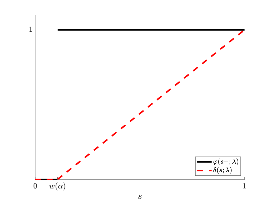
Therefore, δ⁡(s,0)\delta(s;0) is the largest convex function dominated by φ⁡(s−,0)\varphi(s-;0) on [0,1][0,1], and thus is the convex envelope of φ⁡(s−,0)\varphi(s-;0). The left panel of Figure (7) gives a graphical illustration. ∎
Refer to caption

λ=0\lambda=0

Refer to caption

0<λ<∞0<\lambda<\infty

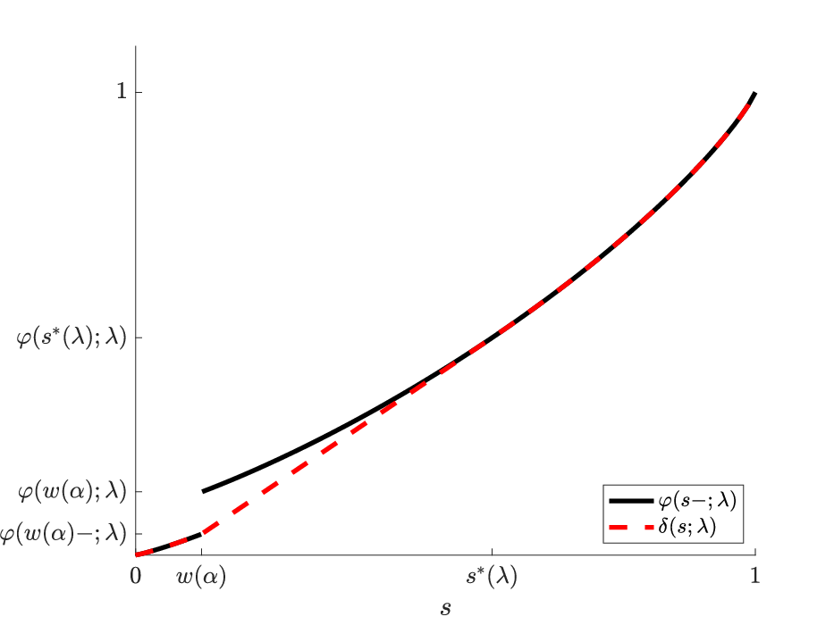
Figure 7: φ⁡(s−,λ)\varphi(s-,\lambda) and δ⁡(s,λ)\delta(s,\lambda) for VaR
Lemma A.2.

If φ\varphi is defined by (A.1) with 0<λ<∞0<\lambda<\infty. Then its convex envelope is given by

δ⁡(s,λ)={φ⁡(s−,λ),0≤s≤w⁡(α),φ⁡(w⁡(α)−,λ)+φ′​(s∗​(λ),λ)​(s−w⁡(α)),w⁡(α)<s≤s∗​(λ),φ⁡(s−,λ),s∗​(λ)<s≤1,\delta(s;\lambda)=\begin{cases}\varphi(s-;\lambda),~&0\leq s\leq w(\alpha),\\ \varphi(w(\alpha)-;\lambda)+\varphi^{\prime}(s^{*}(\lambda);\lambda)(s-w(\alpha)),~&w(\alpha)<s\leq s^{*}(\lambda),\\ \varphi(s-;\lambda),~&s^{*}(\lambda)<s\leq 1,\end{cases}

where s∗​(λ)s^{*}(\lambda) is the unique number in (w⁡(α),1)(w(\alpha),1) such that

φ′​(s∗​(λ)−,λ)=φ⁡(s∗​(λ)−,λ)−φ⁡(w⁡(α)−,λ)s∗​(λ)−w​(α).\varphi^{\prime}(s^{*}(\lambda)-;\lambda)=\frac{\varphi(s^{*}(\lambda)-;\lambda)-\varphi(w(\alpha)-;\lambda)}{s^{*}(\lambda)-w(\alpha)}.
Proof.

Let

f1​(s,λ)=φ⁡(s−,λ)−φ⁡(w⁡(α)−,λ)−φ′​(s,λ)​(s−w⁡(α)),w⁡(α)<s<1,f_{1}(s;\lambda)=\varphi(s-;\lambda)-\varphi(w(\alpha)-;\lambda)-\varphi^{\prime}(s;\lambda)(s-w(\alpha)),~w(\alpha)<s<1,

which is continuous in ss. For w⁡(α)<s1<s2<1w(\alpha)<s_{1}<s_{2}<1, by integration by parts we have

f1​(s1,λ)−f1​(s2,λ)\displaystyle f_{1}(s_{1};\lambda)-f_{1}(s_{2};\lambda)
=\displaystyle= φ⁡(s1−,λ)−φ⁡(s2−,λ)−φ′​(s1,λ)​(s1−w⁡(α))+φ′​(s2,λ)​(s2−w⁡(α))\displaystyle\varphi(s_{1}-;\lambda)-\varphi(s_{2}-;\lambda)-\varphi^{\prime}(s_{1};\lambda)(s_{1}-w(\alpha))+\varphi^{\prime}(s_{2};\lambda)(s_{2}-w(\alpha))
=\displaystyle= −∫s1−s2−dφ(z;λ)+∫s1s2d(zφ′(z;λ))−w(α)(φ′(s2;λ)−φ′(s1;λ))\displaystyle-\int_{s_{1}-}^{s_{2}-}d\varphi(z;\lambda)+\int_{s_{1}}^{s_{2}}d\big(z\varphi^{\prime}(z;\lambda)\big)-w(\alpha)\left(\varphi^{\prime}(s_{2};\lambda)-\varphi^{\prime}(s_{1};\lambda)\right)
=\displaystyle= −∫s1s2φ′(z−;λ)dz+∫s1s2zdφ′(z;λ)+∫s1s2φ′(z;λ)dz−w(α)∫s1s2dφ′(z;λ)\displaystyle-\int_{s_{1}}^{s_{2}}\varphi^{\prime}(z-;\lambda)dz+\int_{s_{1}}^{s_{2}}zd\varphi^{\prime}(z;\lambda)+\int_{s_{1}}^{s_{2}}\varphi^{\prime}(z;\lambda)dz-w(\alpha)\int_{s_{1}}^{s_{2}}d\varphi^{\prime}(z;\lambda)
=\displaystyle= ∫s1s2(z−w⁡(α))​d​φ′​(z,λ)>0,\displaystyle\int_{s_{1}}^{s_{2}}(z-w(\alpha))d\varphi^{\prime}(z;\lambda)>0,

thanks to the convexity of φ⁡(z,λ)\varphi(z;\lambda) on (w⁡(α),1](w(\alpha),1], so f1​(s,λ)f_{1}(s;\lambda) is a strictly decreasing function of ss. Meanwhile,

lims↓w⁡(α)f1​(s,λ)\displaystyle\lim_{s\downarrow w(\alpha)}f_{1}(s;\lambda) =lims↓w⁡(α)1+λ⁡(w−1​(s)−α)−λ​(w−1​(s))′​(s−w⁡(α))1+λ=11+λ,\displaystyle=\lim_{s\downarrow w(\alpha)}\frac{1+\lambda(w^{-1}(s)-\alpha)-\lambda(w^{-1}(s))^{\prime}(s-w(\alpha))}{1+\lambda}=\frac{1}{1+\lambda},

and

lims↑1f1​(s,λ)=φ⁡(1,λ)−φ⁡(w⁡(α)−,λ)−(1−w⁡(α))​lims↑1φ′​(s,λ)=−∞.\lim_{s\uparrow 1}f_{1}(s;\lambda)=\varphi(1;\lambda)-\varphi(w(\alpha)-;\lambda)-(1-w(\alpha))\lim_{s\uparrow 1}\varphi^{\prime}(s;\lambda)=-\infty.

Therefore, there exists a unique s∗​(λ)∈(w⁡(α),1)s^{*}(\lambda)\in(w(\alpha),1) such that f1​(s∗​(λ),λ)=0f_{1}(s^{*}(\lambda);\lambda)=0.

Thanks to the convexity of φ⁡(s,λ)\varphi(s;\lambda) on [0,w⁡(α)][0,w(\alpha)] and on (w⁡(α),1](w(\alpha),1], it is easy to verify that δ⁡(s,λ)\delta(s;\lambda) is a continuous convex function dominated by φ⁡(s−,λ)\varphi(s-;\lambda) on [0,1][0,1]. For any convex function ψ⁡(s)\psi(s) dominated by φ⁡(s−,λ)\varphi(s-;\lambda), it is clearly dominated on [0,w⁡(α)]∪(s∗​(λ),1][0,w(\alpha)]\cup(s^{*}(\lambda),1] by δ⁡(s,λ)\delta(s;\lambda) as δ⁡(s,λ)=φ⁡(s−,λ)\delta(s;\lambda)=\varphi(s-;\lambda). By the same argument as in the proof of Lemma A.1, we have that ψ⁡(s)\psi(s) is dominated by δ⁡(s,λ)\delta(s;\lambda) on (w⁡(α),s∗​(λ)](w(\alpha),s^{*}(\lambda)] too. Therefore, δ⁡(s,λ)\delta(s;\lambda) is the largest convex function dominated by φ⁡(s−,λ)\varphi(s-;\lambda), and thus the convex envelope of φ⁡(s−,λ)\varphi(s-;\lambda). The right panel of Figure (7) gives a graphical illustration. ∎
The following function

φ⁡(s−,λ)={(1α+λ)​w−1​(s)1+λ,0≤s≤w⁡(α)1+λ​w−1​(s)1+λ,w⁡(α)<s≤1.\varphi(s-;\lambda)=\begin{cases}\frac{(\frac{1}{\alpha}+\lambda)w^{-1}(s)}{1+\lambda},~&0\leq s\leq w(\alpha)\\ \frac{1+\lambda w^{-1}(s)}{1+\lambda},~&w(\alpha)<s\leq 1.\end{cases} (A.2)

is increasing, and convex on [0,w⁡(α)][0,w(\alpha)] and on (w⁡(α),1](w(\alpha),1], respectively. It is continuous on [0,1][0,1].

Lemma A.3.

If φ\varphi is defined by (A.2) with λ=0\lambda=0. Then its convex envelope is given by

δ⁡(s,0)={φ⁡(s−,0),0≤s≤t0,φ⁡(t0−,0)+φ′​(t0,0)​(s−t0),t0<s≤1,\delta(s;0)=\begin{cases}\varphi(s-;0),~&0\leq s\leq t_{0},\\ \varphi(t_{0}-;0)+\varphi^{\prime}(t_{0};0)(s-t_{0}),~&t_{0}<s\leq 1,\end{cases}

where t0t_{0} is the unique number in (0,w⁡(α))(0,w(\alpha)) such that

φ′​(t0,0)=1−φ⁡(t0−,0)1−t0.\varphi^{\prime}(t_{0};0)=\frac{1-\varphi(t_{0}-;0)}{1-t_{0}}.
Proof.

When λ=0\lambda=0, we have

φ(s−;0)={1α​w−1​(s),0≤s≤w⁡(α),1,w⁡(α)<s≤1,\varphi(s-;0)=\left\{\begin{aligned} &\frac{1}{\alpha}w^{-1}(s),~&0\leq s\leq w(\alpha),\\ &1,~&w(\alpha)<s\leq 1,\end{aligned}\right.

Let

f2​(s)=1−φ⁡(s−,0)−φ′​(s,0)​(1−s),0<s<w⁡(α).f_{2}(s)=1-\varphi(s-;0)-\varphi^{\prime}(s;0)(1-s),~0<s<w(\alpha).

For 0<s1<s2<w⁡(α)0<s_{1}<s_{2}<w(\alpha), by integration by parts we have

f2​(s1)−f2​(s2)=\displaystyle f_{2}(s_{1})-f_{2}(s_{2})= −φ⁡(s1−,0)+φ⁡(s2−,0)−φ′​(s1,0)​(1−s1)+φ′​(s2,0)​(1−s2)\displaystyle-\varphi(s_{1}-;0)+\varphi(s_{2}-;0)-\varphi^{\prime}(s_{1};0)(1-s_{1})+\varphi^{\prime}(s_{2};0)(1-s_{2})
=\displaystyle= ∫s1s2φ′​(z,0)​dz−∫s1s2d⁡(z​φ′​(z,0))+∫s1s2d​φ′​(z,0)\displaystyle\int_{s_{1}}^{s_{2}}\varphi^{\prime}(z;0)dz-\int_{s_{1}}^{s_{2}}d\big(z\varphi^{\prime}(z;0)\big)+\int_{s_{1}}^{s_{2}}d\varphi^{\prime}(z;0)
=\displaystyle= ∫s1s2(1−z)​d​φ′​(z,0)>0,\displaystyle\int_{s_{1}}^{s_{2}}(1-z)d\varphi^{\prime}(z;0)>0,

again thanks to the convexity of φ⁡(z,0)\varphi(z;0) on [0,w⁡(α)][0,w(\alpha)], so f2​(s)f_{2}(s) is a strictly decreasing function of ss. Moreover, thanks to the strictly convexity of w−1​(s)w^{-1}(s),

lims↑w⁡(α)f2(s)=−1−w⁡(α)αlims↑w⁡(α)(w−1(s))′<0,\lim_{s\uparrow w(\alpha)}f_{2}(s)=-\frac{1-w(\alpha)}{\alpha}\lim_{s\uparrow w(\alpha)}(w^{-1}(s))^{\prime}<0,

and

lims↓0f2​(s)=1−1α​lims↓0(w−1​(s))′=1.\lim_{s\downarrow 0}f_{2}(s)=1-\frac{1}{\alpha}\lim_{s\downarrow 0}(w^{-1}(s))^{\prime}=1.

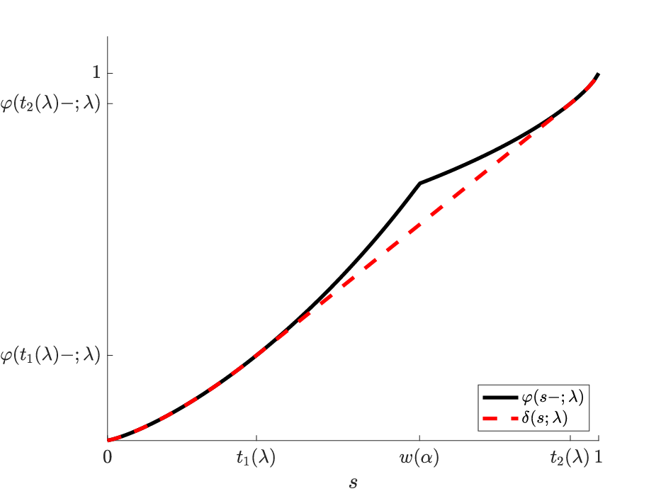
Therefore, there exists a unique t0∈(0,w⁡(α))t_{0}\in(0,w(\alpha)) such that f2​(t0)=0f_{2}(t_{0})=0. By the same argument as in the proof of Lemma A.1, we can show that δ⁡(s−,0)\delta(s-;0) is the convex envelope of φ⁡(s−,0)\varphi(s-;0). The left panel of Figure (8) gives a graphical illustration. ∎
Refer to caption

λ=0\lambda=0

Refer to caption

0<λ<∞0<\lambda<\infty

Figure 8: φ⁡(s−,λ)\varphi(s-,\lambda) and δ⁡(s,λ)\delta(s,\lambda) for ES
Lemma A.4.

If φ\varphi is defined by (A.2) with 0<λ<∞0<\lambda<\infty. Then its convex envelope is given by

δ⁡(s,λ)={φ⁡(s−,λ),0≤s≤t1​(λ),φ⁡(t1​(λ)−,λ)+φ′​(t1​(λ),λ)​(s−t1​(λ)),t1​(λ)<s≤t2​(λ),φ⁡(s−,λ),t2​(λ)<s≤1,\delta(s;\lambda)=\begin{cases}\varphi(s-;\lambda),~&0\leq s\leq t_{1}(\lambda),\\ \varphi(t_{1}(\lambda)-;\lambda)+\varphi^{\prime}(t_{1}(\lambda);\lambda)(s-t_{1}(\lambda)),~&t_{1}(\lambda)<s\leq t_{2}(\lambda),\\ \varphi(s-;\lambda),~&t_{2}(\lambda)<s\leq 1,\end{cases}

where 0<t1​(λ)<w⁡(α)<t2​(λ)<10<t_{1}(\lambda)<w(\alpha)<t_{2}(\lambda)<1 are the unique pair such that

{φ′​(t1​(λ),λ)=φ′​(t2​(λ),λ)φ′​(t1​(λ),λ)=φ⁡(t2−,λ)−φ⁡(t1−,λ)t2−t1.\begin{cases}\varphi^{\prime}(t_{1}(\lambda);\lambda)=\varphi^{\prime}(t_{2}(\lambda);\lambda)\\ \varphi^{\prime}(t_{1}(\lambda);\lambda)=\frac{\varphi(t_{2}-;\lambda)-\varphi(t_{1}-;\lambda)}{t_{2}-t_{1}}.\end{cases} (A.3)
Proof.

Again by the same argument as in the proof of Lemma A.1, we can show that δ⁡(s−,λ)\delta(s-;\lambda) is the convex envelope of φ⁡(s−,λ)\varphi(s-;\lambda). The right panel of Figure (8) gives a graphical illustration. It is only left to show the existence and uniqueness of the pair 0<t1​(λ)<w⁡(α)<t2​(λ)<10<t_{1}(\lambda)<w(\alpha)<t_{2}(\lambda)<1 that satisfies (A.3).

Let

s¯​(λ)=w⁡(1−Fξ​(1α+λλ​Gξ​(1−α))).\underline{s}(\lambda)=w\left(1-F_{\xi}\left(\tfrac{\frac{1}{\alpha}+\lambda}{\lambda}G_{\xi}\left(1-\alpha\right)\right)\right).

In view of the strict monotonicity of ww and FξF_{\xi} and positivity of GξG_{\xi}, we have

s¯​(λ)<w⁡(1−Fξ​(Gξ​(1−α)))=w⁡(α).\underline{s}(\lambda)<w\left(1-F_{\xi}\big(G_{\xi}(1-\alpha)\big)\right)=w(\alpha).

Define

y⁡(s)=w⁡(1−Fξ​(λ1α+λ​Gξ​(1−w−1​(s)))),s∈(s¯​(λ),w⁡(α)).y(s)=w\left(1-F_{\xi}\left(\tfrac{\lambda}{\frac{1}{\alpha}+\lambda}G_{\xi}\big(1-w^{-1}(s)\big)\right)\right),\quad s\in(\underline{s}(\lambda),w(\alpha)).

Then by monotonicity, for s∈(s¯​(λ),w​(α))s\in(\underline{s}(\lambda),w(\alpha)),

y⁡(s)\displaystyle y(s) =w⁡(1−Fξ​(λ1α+λ​Gξ​(1−w−1​(s))))\displaystyle=w\left(1-F_{\xi}\left(\tfrac{\lambda}{\frac{1}{\alpha}+\lambda}G_{\xi}\big(1-w^{-1}(s)\big)\right)\right)
>w⁡(1−Fξ​(λ1α+λ​Gξ​(1−w−1​(s¯​(λ)))))\displaystyle>w\left(1-F_{\xi}\left(\tfrac{\lambda}{\frac{1}{\alpha}+\lambda}G_{\xi}\big(1-w^{-1}(\underline{s}(\lambda))\big)\right)\right)
=w⁡(1−Fξ​(λ1α+λ​Gξ​(Fξ​(1α+λλ​Gξ​(1−α)))))\displaystyle=w\left(1-F_{\xi}\left(\tfrac{\lambda}{\frac{1}{\alpha}+\lambda}G_{\xi}\left(F_{\xi}\left(\tfrac{\frac{1}{\alpha}+\lambda}{\lambda}G_{\xi}\left(1-\alpha\right)\right)\right)\right)\right)
=w⁡(1−Fξ​(Gξ​(1−α)))\displaystyle=w\left(1-F_{\xi}\left(G_{\xi}\left(1-\alpha\right)\right)\right)
=w⁡(α).\displaystyle=w(\alpha).

and it is not hard to verify that

φ′​(s,λ)=φ′​(y⁡(s),λ).\displaystyle\varphi^{\prime}(s;\lambda)=\varphi^{\prime}(y(s);\lambda). (A.4)

Let

f3​(s,λ)=φ⁡(y⁡(s)−,λ)−φ⁡(s−,λ)−φ′​(s,λ)​(y⁡(s)−s),0<s<w⁡(α).f_{3}(s;\lambda)=\varphi(y(s)-;\lambda)-\varphi(s-;\lambda)-\varphi^{\prime}(s;\lambda)(y(s)-s),~0<s<w(\alpha).

For s¯​(λ)<s1<s2<w⁡(α)\underline{s}(\lambda)<s_{1}<s_{2}<w(\alpha), thanks to (A.4) and using integration by parts, we have

f3​(s1,λ)−f3​(s2,λ)\displaystyle\quad\;f_{3}(s_{1};\lambda)-f_{3}(s_{2};\lambda)
=φ⁡(y⁡(s1)−,λ)−φ⁡(y⁡(s2)−,λ)−(φ⁡(s1−,λ)−φ⁡(s2−,λ))\displaystyle=\varphi(y(s_{1})-;\lambda)-\varphi(y(s_{2})-;\lambda)-(\varphi(s_{1}-;\lambda)-\varphi(s_{2}-;\lambda))
−φ′​(s1,λ)​(y⁡(s1)−s1)+φ′​(s2,λ)​(y⁡(s2)−s2)\displaystyle\quad\;-\varphi^{\prime}(s_{1};\lambda)(y(s_{1})-s_{1})+\varphi^{\prime}(s_{2};\lambda)(y(s_{2})-s_{2})
=−∫y⁡(s1)y⁡(s2)dφ(z−;λ)+∫s1s2d(φ′(z;λ)y(z))+∫s1s2dφ(z−;λ)−∫s1s2d(φ′(z;λ)z)\displaystyle=-\int_{y(s_{1})}^{y(s_{2})}d\varphi(z-;\lambda)+\int_{s_{1}}^{s_{2}}d\big(\varphi^{\prime}(z;\lambda)y(z)\big)+\int_{s_{1}}^{s_{2}}d\varphi(z-;\lambda)-\int_{s_{1}}^{s_{2}}d\big(\varphi^{\prime}(z;\lambda)z\big)
=−∫y⁡(s1)y⁡(s2)φ′(z;λ)dz+∫s1s2d(φ′(y(z);λ)y(z))−∫s1s2zdφ′(z;λ)\displaystyle=-\int_{y(s_{1})}^{y(s_{2})}\varphi^{\prime}(z;\lambda)dz+\int_{s_{1}}^{s_{2}}d\big(\varphi^{\prime}(y(z);\lambda)y(z)\big)-\int_{s_{1}}^{s_{2}}zd\varphi^{\prime}(z;\lambda)
=−∫y⁡(s1)y⁡(s2)φ′(z;λ)dz+∫y⁡(s1)y⁡(s2)d(φ′(z;λ)z)−∫s1s2zdφ′(z;λ)\displaystyle=-\int_{y(s_{1})}^{y(s_{2})}\varphi^{\prime}(z;\lambda)dz+\int_{y(s_{1})}^{y(s_{2})}d\big(\varphi^{\prime}(z;\lambda)z\big)-\int_{s_{1}}^{s_{2}}zd\varphi^{\prime}(z;\lambda)
=∫y⁡(s1)y⁡(s2)z​d​φ′​(z,λ)−∫s1s2z​d​φ′​(z,λ)\displaystyle=\int_{y(s_{1})}^{y(s_{2})}zd\varphi^{\prime}(z;\lambda)-\int_{s_{1}}^{s_{2}}zd\varphi^{\prime}(z;\lambda)
=∫s1s2y⁡(z)​d​φ′​(y⁡(z),λ)+∫s1s2z​d​φ′​(z,λ)\displaystyle=\int_{s_{1}}^{s_{2}}y(z)d\varphi^{\prime}(y(z);\lambda)+\int_{s_{1}}^{s_{2}}zd\varphi^{\prime}(z;\lambda)
=∫s1s2(y⁡(z)−z)​d​φ′​(z,λ)>0\displaystyle=\int_{s_{1}}^{s_{2}}(y(z)-z)d\varphi^{\prime}(z;\lambda)>0

by virtue of y⁡(z)>w⁡(α)>zy(z)>w(\alpha)>z for z∈(s¯​(λ),w​(α))z\in(\underline{s}(\lambda),w(\alpha)) and φ\varphi is convex on (0,w⁡(α))(0,w(\alpha)), so f3​(s,λ)f_{3}(s;\lambda) is a strictly decreasing function of ss. Moreover, thanks to the strictly convexity of φ\varphi (0,w⁡(α))(0,w(\alpha)) and on (w⁡(α),1)(w(\alpha),1), respectively, and the fact that lims↓s¯​(λ)y⁡(s)=w⁡(α)\lim_{s\downarrow\underline{s}(\lambda)}y(s)=w(\alpha), we have

lims↓s¯​(λ)f3​(s,λ)=\displaystyle\lim_{s\downarrow\underline{s}(\lambda)}f_{3}(s;\lambda)= lims↓s¯​(λ)(∫w⁡(α)y⁡(s)φ′​(z,λ)​dz+∫sw⁡(α)φ′​(z,λ)​dz−φ′​(s,λ)​(y⁡(s)−s))\displaystyle\lim_{s\downarrow\underline{s}(\lambda)}\left(\int_{w(\alpha)}^{y(s)}\varphi^{\prime}(z;\lambda)dz+\int_{s}^{w(\alpha)}\varphi^{\prime}(z;\lambda)dz-\varphi^{\prime}(s;\lambda)\left(y(s)-s\right)\right)
=\displaystyle= ∫s¯​(λ)w⁡(α)φ′​(z,λ)​dz−φ′​(s¯​(λ),λ)​(w⁡(α)−s¯​(λ))\displaystyle\int_{\underline{s}(\lambda)}^{w(\alpha)}\varphi^{\prime}(z;\lambda)dz-\varphi^{\prime}(\underline{s}(\lambda);\lambda)\left(w(\alpha)-\underline{s}(\lambda)\right)
=\displaystyle= ∫s¯​(λ)w⁡(α)(φ′​(z,λ)−φ′​(s¯​(λ),λ))​dz>0,\displaystyle\int_{\underline{s}(\lambda)}^{w(\alpha)}\left(\varphi^{\prime}(z;\lambda)-\varphi^{\prime}(\underline{s}(\lambda);\lambda)\right)dz>0,

and

lims↑w⁡(α)f3​(s,λ)=\displaystyle\lim_{s\uparrow w(\alpha)}f_{3}(s;\lambda)= lims↑w⁡(α)(∫w⁡(α)y⁡(s)φ′​(z,λ)​dz+∫sw⁡(α)φ′​(z,λ)​dz−φ′​(s,λ)​(y⁡(s)−s))\displaystyle\lim_{s\uparrow w(\alpha)}\left(\int_{w(\alpha)}^{y(s)}\varphi^{\prime}(z;\lambda)dz+\int_{s}^{w(\alpha)}\varphi^{\prime}(z;\lambda)dz-\varphi^{\prime}(s;\lambda)\left(y(s)-s\right)\right)
=\displaystyle= ∫w⁡(α)y⁡(w⁡(α)−)φ′​(z,λ)​dz−φ′​(w⁡(α)−,λ)​(y⁡(w⁡(α)−)−w⁡(α))\displaystyle\int_{w(\alpha)}^{y(w(\alpha)-)}\varphi^{\prime}(z;\lambda)dz-\varphi^{\prime}(w(\alpha)-;\lambda)\left(y(w(\alpha)-)-w(\alpha)\right)
=\displaystyle= ∫w⁡(α)y⁡(w⁡(α)−)(φ′​(z,λ)−φ′​(y⁡(w⁡(α)−),λ))​dz<0.\displaystyle\int_{w(\alpha)}^{y(w(\alpha)-)}\left(\varphi^{\prime}(z;\lambda)-\varphi^{\prime}(y(w(\alpha)-);\lambda)\right)dz<0.

Therefore, there exists a unique t1​(λ)∈(s¯​(λ),w⁡(α))t_{1}(\lambda)\in(\underline{s}(\lambda),w(\alpha)) that solves f3​(t1​(λ),λ)=0f_{3}(t_{1}(\lambda);\lambda)=0. Let t2​(λ)=y⁡(t1​(λ))t_{2}(\lambda)=y(t_{1}(\lambda)). Then, t1​(λ)t_{1}(\lambda) and t2​(λ)t_{2}(\lambda) solve (A.3). ∎

Appendix B Proofs

Proof of Lemma 3.1.

This is indeed contained in the proof of Theorem 7, Xu, 2014. We give it here to make the paper self-contained. Suppose XT∗X_{T}^{*} is optimal to (2.8) and 𝔼⁡[ξT​XT∗]<x{\mathbb{E}}[\xi_{T}X_{T}^{*}]<x. Define

X~T=XT∗+x−𝔼⁡[ξT​XT∗]𝔼⁡[ξT],\tilde{X}_{T}=X_{T}^{*}+\frac{x-{\mathbb{E}}[\xi_{T}X_{T}^{*}]}{{\mathbb{E}}[\xi_{T}]},

which satisfies the budget constraint. Clearly X~T>XT∗\tilde{X}_{T}>X_{T}^{*}. Let RT∗R_{T}^{*} and R~T\tilde{R}_{T} be the corresponding log-returns of XT∗X_{T}^{*} and X~T\tilde{X}_{T}, respectively. Then

R~T\displaystyle\tilde{R}_{T} >RT∗,a.s.,\displaystyle>R_{T}^{*},~a.s.,
𝔼⁡[R~T]\displaystyle{\mathbb{E}}[\tilde{R}_{T}] >𝔼⁡[RT∗],\displaystyle>{\mathbb{E}}[R_{T}^{*}],
ρΦ​(R~T)\displaystyle\rho_{\Phi}(\tilde{R}_{T}) <ρΦ​(RT∗),\displaystyle<\rho_{\Phi}(R_{T}^{*}),

and consequently

λ​𝔼​[R~T]−ρΦ​(R~T)>λ​𝔼​[RT∗]−ρΦ​(RT∗),\lambda{\mathbb{E}}[\tilde{R}_{T}]-\rho_{\Phi}(\tilde{R}_{T})>\lambda{\mathbb{E}}[R_{T}^{*}]-\rho_{\Phi}(R_{T}^{*}),

contradicting the optimality of XT∗X_{T}^{*} to (2.8). ∎

Proof of Proposition 3.1.

We handle the two cases 0<λ<∞0<\lambda<\infty and λ=0\lambda=0 separately.

Case 0<λ<∞0<\lambda<\infty.

Define

ℍ1={H∈𝔾:H(s)>0,∀s∈(0,1]}∩ℍΦ.\mathbb{H}_{1}=\big\{H\in\mathbb{G}\colon H(s)>0,~\forall s\in(0,1]\big\}\cap\mathbb{H}_{\Phi}.

It suffices to consider the following optimization problem

maxH∈ℍ1⁡L⁡(H⁡(⋅),λ,η),\max_{H\in\mathbb{H}_{1}}L(H(\cdot);\lambda,\eta),

as L⁡(H⁡(⋅),λ,η)=−∞,L(H(\cdot);\lambda,\eta)=-\infty, if H∈𝔾∖ℍ1H\in\mathbb{G}\setminus\mathbb{H}_{1}.

Because δ⁡(s,λ)\delta(s;\lambda) is the convex envelope of φ⁡(s−,λ)\varphi(s-;\lambda), φ⁡(s−,λ)≥δ⁡(s,λ),s∈[0,1]\varphi(s-;\lambda)\geq\delta(s;\lambda),~s\in[0,1], δ⁡(0,λ)=φ⁡(0−,λ)=0\delta(0;\lambda)=\varphi(0-;\lambda)=0, and δ⁡(1,λ)=φ⁡(1−,λ)=1\delta(1;\lambda)=\varphi(1-;\lambda)=1. For any H∈ℍ1H\in\mathbb{H}_{1}, we have

∫[0,1)(φ⁡(s−,λ)−δ⁡(s,λ))​d​ln⁡H⁡(s)≥0.\int_{[0,1)}(\varphi(s-;\lambda)-\delta(s;\lambda))d\ln H(s)\geq 0.

From Fubini’s theorem, we have

∫[0,1)(φ⁡(s−,λ)−δ⁡(s,λ))​d​ln⁡H⁡(s)\displaystyle\int_{[0,1)}\big(\varphi(s-;\lambda)-\delta(s;\lambda)\big)d\ln H(s)
=\displaystyle= ∫[0,1)ln⁡H⁡(s)​dδ​(s,λ)−∫[0,1)ln⁡H⁡(s)​dφ​(s,λ)≥0.\displaystyle\int_{[0,1)}\ln H(s)d\delta(s;\lambda)-\int_{[0,1)}\ln H(s)d\varphi(s;\lambda)\geq 0.

and consequently

L⁡(H⁡(⋅),λ,η)\displaystyle L(H(\cdot);\lambda,\eta) =(1+λ)​∫[0,1)ln⁡H⁡(s)​𝑑φ​(s,λ)−η​∫[0,1)H⁡(s)​𝑑s\displaystyle=(1+\lambda)\int_{[0,1)}\ln H(s)d\varphi(s;\lambda)-\eta\int_{[0,1)}H(s)ds
≤(1+λ)​∫[0,1)ln⁡H⁡(s)​𝑑δ​(s,λ)−η​∫[0,1)H⁡(s)​𝑑s\displaystyle\leq(1+\lambda)\int_{[0,1)}\ln H(s)d\delta(s;\lambda)-\eta\int_{[0,1)}H(s)ds
=(1+λ)​∫[0,1)ln⁡(H⁡(s))​δ′​(s,λ)​𝑑s−η​∫[0,1)H⁡(s)​𝑑s\displaystyle=(1+\lambda)\int_{[0,1)}\ln\left(H(s)\right)\delta^{\prime}(s;\lambda)ds-\eta\int_{[0,1)}H(s)ds
≤(1+λ)​∫[0,1)ln⁡(H∗​(s,λ,η))​δ′​(s,λ)​𝑑s−η​∫[0,1)H∗​(s,λ,η)​𝑑s,\displaystyle\leq(1+\lambda)\int_{[0,1)}\ln\left(H^{*}(s;\lambda,\eta)\right)\delta^{\prime}(s;\lambda)ds-\eta\int_{[0,1)}H^{*}(s;\lambda,\eta)ds,

where H∗​(s,λ,η)=1+λη​δ′​(s,λ)H^{*}(s;\lambda,\eta)=\frac{1+\lambda}{\eta}\delta^{\prime}(s;\lambda) is given by point-wise optimization. We then show that

L⁡(H∗​(⋅,λ,η),λ,η)=(1+λ)​∫[0,1)ln⁡(H∗​(s,λ,η))​δ′​(s,λ)​𝑑s−η​∫[0,1)H∗​(s,λ,η)​𝑑s,L(H^{*}(\cdot;\lambda,\eta);\lambda,\eta)=(1+\lambda)\int_{[0,1)}\ln\left(H^{*}(s;\lambda,\eta)\right)\delta^{\prime}(s;\lambda)ds-\eta\int_{[0,1)}H^{*}(s;\lambda,\eta)ds,

which is equivalent to

∫[0,1)ln⁡H∗​(s,λ,η)​𝑑φ​(s,λ)=∫[0,1)ln⁡H∗​(s,λ,η)​𝑑δ​(s,λ),\int_{[0,1)}\ln H^{*}(s;\lambda,\eta)d\varphi(s;\lambda)=\int_{[0,1)}\ln H^{*}(s;\lambda,\eta)d\delta(s;\lambda),

or by Fubini’s theorem,

∫(0,1)(φ⁡(s−,λ)−δ⁡(s,λ))​d​ln⁡H∗​(s,λ,η)=0,\int_{(0,1)}\big(\varphi(s-;\lambda)-\delta(s;\lambda)\big)d\ln H^{*}(s;\lambda,\eta)=0,

namely,

∫(0,1)(φ⁡(s−,λ)−δ⁡(s,λ))​d​ln⁡(δ′​(s,λ))=0.\int_{(0,1)}\big(\varphi(s-;\lambda)-\delta(s;\lambda)\big)d\ln\big(\delta^{\prime}(s;\lambda)\big)=0. (B.1)

Because δ′​(s,λ)\delta^{\prime}(s;\lambda) is constant on any sub-interval of {s∈(0,1):φ⁡(s−,λ)>δ⁡(s,λ)}\{s\in(0,1):\varphi(s-;\lambda)>\delta(s;\lambda)\}, the above identity (B.1) holds.

Finally, we need to verify H∗​(⋅,λ,η)∈ℍ1H^{*}(\cdot;\lambda,\eta)\in\mathbb{H}_{1}. If Φ⁡({0})=0\Phi(\{0\})=0, then

ℍ1={H∈𝔾:H(s)>0,∀s∈(0,1]};\mathbb{H}_{1}=\big\{H\in\mathbb{G}\colon H(s)>0,~\forall s\in(0,1]\big\};

if Φ⁡({0})>0\Phi(\{0\})>0, then

ℍ1={H∈𝔾:H⁡(0)>0}.\mathbb{H}_{1}=\big\{H\in\mathbb{G}\colon H(0)>0\big\}.

Because 0<λ<∞0<\lambda<\infty, φ⁡(s−,λ)>0\varphi(s-;\lambda)>0 for s>0s>0. We claim δ′​(s,λ)>0\delta^{\prime}(s;\lambda)>0 for s>0s>0. Otherwise, we have

s1=sup{s∈[0,1]:δ′​(s,λ)=0}>0.s_{1}=\sup\big\{s\in[0,1]\colon\delta^{\prime}(s;\lambda)=0\big\}>0.

Since δ⁡(1,λ)>δ⁡(0,λ)\delta(1;\lambda)>\delta(0;\lambda), we have s1<1s_{1}<1. It follows from the convexity of δ⁡(s,λ)\delta(s;\lambda) that δ′​(s,λ)=0\delta^{\prime}(s;\lambda)=0 for s<s1s<s_{1} and δ′​(s,λ)>0\delta^{\prime}(s;\lambda)>0 for s>s1s>s_{1}. This means δ⁡(s,λ)\delta(s;\lambda) is not affine around s1s_{1}. But φ⁡(s1−,λ)>0=δ⁡(s1,λ)\varphi(s_{1}-;\lambda)>0=\delta(s_{1};\lambda), so δ⁡(s,λ)\delta(s;\lambda) should be affine in the neighborhood of s1s_{1}, leading to a contradiction.

We need to additionally show δ′​(0,λ)>0\delta^{\prime}(0;\lambda)>0 if Φ⁡({0})=0\Phi(\{0\})=0. In fact, φ⁡(0,λ)>φ⁡(0−,λ)=δ⁡(0,λ)=0\varphi(0;\lambda)>\varphi(0-;\lambda)=\delta(0;\lambda)=0. If δ′​(0,λ)=0\delta^{\prime}(0;\lambda)=0, then φ⁡(s−,λ)>δ⁡(s,λ)\varphi(s-;\lambda)>\delta(s;\lambda) and δ⁡(s,λ)\delta(s;\lambda) is affine for ss sufficiently close to 00, which contradicts the fact δ′​(s,λ)>0\delta^{\prime}(s;\lambda)>0 for s>0s>0.

Case λ=0\lambda=0.

In view of (2.6), we need to solve the following optimization problem

maxH∈ℍΦ⁡L⁡(H⁡(⋅),0,η).\max_{H\in\mathbb{H}_{\Phi}}~L(H(\cdot);0,\eta).

Let

zΦ=sup{z∈[0,1]:Φ⁡([0,z])=0}.z_{\Phi}=\sup\big\{z\in[0,1]\colon\Phi([0,z])=0\big\}.

We then have Φ⁡([0,zΦ))=0\Phi([0,z_{\Phi}))=0 and φ⁡(z−,0)=Φ⁡([0,w−1​(z)))=0\varphi(z-;0)=\Phi([0,w^{-1}(z)))=0, for all z∈[0,w⁡(zΦ)]z\in[0,w(z_{\Phi})]. According to (3.5), we know that δ⁡(z,0)=φ⁡(z−,0)=0\delta(z;0)=\varphi(z-;0)=0, for all z∈[0,w⁡(zΦ)]z\in[0,w(z_{\Phi})]. There are two subcases.

  • •

    If Φ⁡({zΦ})>0\Phi(\{z_{\Phi}\})>0, then ℍΦ={H∈𝔾:H⁡(w⁡(zΦ))>0}\mathbb{H}_{\Phi}=\{H\in\mathbb{G}\colon H(w(z_{\Phi}))>0\} and

    L⁡(H⁡(⋅),0,η)=\displaystyle L(H(\cdot);0,\eta)= ∫[w⁡(zΦ),1)ln⁡H⁡(s)​𝑑φ​(s,0)−η​∫[0,1)H⁡(s)​𝑑s\displaystyle\int_{[w(z_{\Phi}),1)}\ln H(s)d\varphi(s;0)-\eta\int_{[0,1)}H(s)ds
    =\displaystyle= ∫[w⁡(zΦ),1)ln⁡H⁡(s)​dΦ​([0,w−1​(s)])−η​∫[0,1)H⁡(s)​ds.\displaystyle\int_{[w(z_{\Phi}),1)}\ln H(s)d\Phi([0,w^{-1}(s)])-\eta\int_{[0,1)}H(s)ds.

    Similar to the case 0<λ<∞0<\lambda<\infty, we can show, for any H∈ℍΦH\in\mathbb{H}_{\Phi},

    ∫[w⁡(zΦ),1)ln⁡H⁡(s)​dδ​(s,λ)−∫[w⁡(zΦ),1)ln⁡H⁡(s)​dφ​(s,λ)\displaystyle\int_{[w(z_{\Phi}),1)}\ln H(s)d\delta(s;\lambda)-\int_{[w(z_{\Phi}),1)}\ln H(s)d\varphi(s;\lambda)
    =\displaystyle= ∫[w⁡(zΦ),1)(φ⁡(s−,λ)−δ⁡(s,λ))​d​ln⁡H⁡(s)≥0.\displaystyle\int_{[w(z_{\Phi}),1)}\big(\varphi(s-;\lambda)-\delta(s;\lambda)\big)d\ln H(s)\geq 0.

    We then have

    L⁡(H⁡(⋅),0,η)=\displaystyle L(H(\cdot);0,\eta)= ∫[w⁡(zΦ),1)ln⁡H⁡(s)​𝑑φ​(s,0)−η​∫[0,1)H⁡(s)​𝑑s\displaystyle\int_{[w(z_{\Phi}),1)}\ln H(s)d\varphi(s;0)-\eta\int_{[0,1)}H(s)ds
    ≤\displaystyle\leq ∫[w⁡(zΦ),1)ln⁡H⁡(s)​𝑑δ​(s,0)−η​∫[0,1)H⁡(s)​𝑑s\displaystyle\int_{[w(z_{\Phi}),1)}\ln H(s)d\delta(s;0)-\eta\int_{[0,1)}H(s)ds
    =\displaystyle= ∫[w⁡(zΦ),1)ln⁡(H⁡(s))​δ′​(s,0)​𝑑s−η​∫[0,1)H⁡(s)​𝑑s\displaystyle\int_{[w(z_{\Phi}),1)}\ln\left(H(s)\right)\delta^{\prime}(s;0)ds-\eta\int_{[0,1)}H(s)ds
    ≤\displaystyle\leq ∫[w⁡(zΦ),1)ln⁡(H∗​(s,0,η))​δ′​(s,λ)​ds−η​∫[0,1)H∗​(s,0,η)​ds,\displaystyle\int_{[w(z_{\Phi}),1)}\ln\left(H^{*}(s;0,\eta)\right)\delta^{\prime}(s;\lambda)ds-\eta\int_{[0,1)}H^{*}(s;0,\eta)ds,

    where

    H∗​(s,λ,η)=1η​δ′​(s,λ)={0,0≤z<w⁡(zΦ),1η​δ′​(s,λ),w⁡(zΦ)≤z≤1,H^{*}(s;\lambda,\eta)=\frac{1}{\eta}\delta^{\prime}(s;\lambda)=\begin{cases}0,~&0\leq z<w(z_{\Phi}),\\ \frac{1}{\eta}\delta^{\prime}(s;\lambda),~&w(z_{\Phi})\leq z\leq 1,\end{cases}

    is given by point-wise optimization. We can similarly show

    L⁡(H∗​(⋅,0,η),0,η)=∫[w⁡(zΦ),1)ln⁡(H∗​(s,0,η))​δ′​(s,0)​𝑑s−η​∫[0,1)H∗​(s,0,η)​𝑑sL(H^{*}(\cdot;0,\eta);0,\eta)=\int_{[w(z_{\Phi}),1)}\ln\left(H^{*}(s;0,\eta)\right)\delta^{\prime}(s;0)ds-\eta\int_{[0,1)}H^{*}(s;0,\eta)ds

    by verifying

    ∫(w⁡(zΦ),1)(φ⁡(s−,0)−δ⁡(s,0))​d​ln⁡(δ′​(s,0))=0.\int_{(w(z_{\Phi}),1)}\big(\varphi(s-;0)-\delta(s;0)\big)d\ln\big(\delta^{\prime}(s;0)\big)=0.

    We now verify H∗​(⋅,λ,η)∈ℍΦH^{*}(\cdot;\lambda,\eta)\in\mathbb{H}_{\Phi} by showing δ′​(w⁡(zΦ),λ)>0\delta^{\prime}(w(z_{\Phi});\lambda)>0. Similar to the case 0<λ<∞0<\lambda<\infty, we can show δ′​(s,0)>0\delta^{\prime}(s;0)>0 for s>w⁡(zΦ)s>w(z_{\Phi}). Because φ⁡(w⁡(zΦ),0)>φ⁡(w⁡(zΦ)−,0)=δ⁡(w⁡(zΦ),0)=0\varphi(w(z_{\Phi});0)>\varphi(w(z_{\Phi})-;0)=\delta(w(z_{\Phi});0)=0, we can prove δ′​(w⁡(zΦ),0)>0\delta^{\prime}(w(z_{\Phi});0)>0 in a similar fashion.

  • •

    If Φ⁡({zΦ})=0\Phi(\{z_{\Phi}\})=0, then δ⁡(w⁡(zΦ),0)=φ⁡(w⁡(zΦ)−,0)=φ⁡(w⁡(zΦ),0)=0\delta(w(z_{\Phi});0)=\varphi(w(z_{\Phi})-;0)=\varphi(w(z_{\Phi});0)=0, ℍΦ={H∈𝔾:H(s)>0,∀s>w(zΦ)}\mathbb{H}_{\Phi}=\{H\in\mathbb{G}\colon H(s)>0,~\forall s>w(z_{\Phi})\} and

    L⁡(H⁡(⋅),0,η)=∫(w⁡(zΦ),1)ln⁡H⁡(s)​𝑑φ​(s,0)−η​∫[0,1)H⁡(s)​𝑑s.L(H(\cdot);0,\eta)=\int_{(w(z_{\Phi}),1)}\ln H(s)d\varphi(s;0)-\eta\int_{[0,1)}H(s)ds.

    Similar to the case λ=0\lambda=0 and Φ⁡({zΦ})>0\Phi(\{z_{\Phi}\})>0, we can show, for any H∈ℍΦH\in\mathbb{H}_{\Phi},

    L⁡(H⁡(⋅),0,η)\displaystyle L(H(\cdot);0,\eta) =∫(w⁡(zΦ),1)ln⁡H⁡(s)​𝑑φ​(s,0)−η​∫[0,1)H⁡(s)​𝑑s\displaystyle=\int_{(w(z_{\Phi}),1)}\ln H(s)d\varphi(s;0)-\eta\int_{[0,1)}H(s)ds
    ≤∫(w⁡(zΦ),1)ln⁡H⁡(s)​𝑑δ​(s,0)−η​∫[0,1)H⁡(s)​𝑑s\displaystyle\leq\int_{(w(z_{\Phi}),1)}\ln H(s)d\delta(s;0)-\eta\int_{[0,1)}H(s)ds
    ≤∫(w⁡(zΦ),1)ln⁡(H∗​(s,0,η))​δ′​(s,λ)​𝑑s−η​∫[0,1)H∗​(s,0,η)​𝑑s,\displaystyle\leq\int_{(w(z_{\Phi}),1)}\ln\left(H^{*}(s;0,\eta)\right)\delta^{\prime}(s;\lambda)ds-\eta\int_{[0,1)}H^{*}(s;0,\eta)ds,

    where

    H∗​(s,λ,η)=1η​δ′​(s,λ)={0,0≤z<w⁡(zΦ),1η​δ′​(s,λ),w⁡(zΦ)≤z≤1,H^{*}(s;\lambda,\eta)=\frac{1}{\eta}\delta^{\prime}(s;\lambda)=\begin{cases}0,~&0\leq z<w(z_{\Phi}),\\ \frac{1}{\eta}\delta^{\prime}(s;\lambda),~&w(z_{\Phi})\leq z\leq 1,\end{cases}

    is given by point-wise optimization. We can similarly show

    L⁡(H∗​(⋅,0,η),0,η)=∫(w⁡(zΦ),1)ln⁡(H∗​(s,0,η))​δ′​(s,0)​𝑑s−η​∫[0,1)H∗​(s,0,η)​𝑑s.L(H^{*}(\cdot;0,\eta);0,\eta)=\int_{(w(z_{\Phi}),1)}\ln\left(H^{*}(s;0,\eta)\right)\delta^{\prime}(s;0)ds-\eta\int_{[0,1)}H^{*}(s;0,\eta)ds.

    Finally, it is easy to verify δ′​(s,λ)>0\delta^{\prime}(s;\lambda)>0 for s>w⁡(zΦ)s>w(z_{\Phi}) and thus H∗​(⋅,0,η)∈ℍΦH^{*}(\cdot;0,\eta)\in\mathbb{H}_{\Phi}.

The proof is complete. ∎

Proof of Proposition 3.2.

For any H∈𝔾H\in\mathbb{G} that satisfies the budget constraint in (3.3), we have

λ​∫[0,1)ln⁡H⁡(s)​d​w−1​(s)+∫[0,1)ln⁡H⁡(s)​𝑑Φ​([0,w−1​(s)])\displaystyle\quad\;\lambda\int_{[0,1)}\ln H(s)dw^{-1}(s)+\int_{[0,1)}\ln H(s)d\Phi([0,w^{-1}(s)])
=L⁡(H⁡(⋅),λ,1+λx​𝔼​[ξT])+1+λx​𝔼​[ξT]​∫[0,1)H⁡(s)​𝑑s\displaystyle=L\left(H(\cdot);\lambda,\frac{1+\lambda}{x}{\mathbb{E}}[\xi_{T}]\right)+\frac{1+\lambda}{x}{\mathbb{E}}[\xi_{T}]\int_{[0,1)}H(s)ds
=L⁡(H⁡(⋅),λ,1+λx​𝔼​[ξT])+(1+λ).\displaystyle=L\left(H(\cdot);\lambda,\frac{1+\lambda}{x}{\mathbb{E}}[\xi_{T}]\right)+(1+\lambda).

Similarly,

λ​∫[0,1)ln⁡H∗​(s,λ,1+λx​𝔼​[ξT])​d​w−1​(s)\displaystyle\quad\;\lambda\int_{[0,1)}\ln H^{*}\left(s;\lambda,\frac{1+\lambda}{x}{\mathbb{E}}[\xi_{T}]\right)dw^{-1}(s)
+∫[0,1)lnH∗(s;λ,1+λx𝔼[ξT])dΦ([0,w−1(s)])\displaystyle\quad\quad+\int_{[0,1)}\ln H^{*}\left(s;\lambda,\frac{1+\lambda}{x}{\mathbb{E}}[\xi_{T}]\right)d\Phi([0,w^{-1}(s)])
=L⁡(H∗​(⋅,λ,1+λx​𝔼​[ξT]),λ,1+λx​𝔼​[ξT])+(1+λ).\displaystyle=L\left(H^{*}\left(\cdot;\lambda,\frac{1+\lambda}{x}{\mathbb{E}}[\xi_{T}]\right);\lambda,\frac{1+\lambda}{x}{\mathbb{E}}[\xi_{T}]\right)+(1+\lambda).

By virtue of Proposition 3.1, the claim is proved. ∎

Proof of Proposition 4.1.

First, we have

φ⁡(s−,λ)=Φ⁡([0,w−1​(s)))+λ​w−1​(s)1+λ={λ​w−1​(s)1+λ,0≤s≤w⁡(α),1+λ​w−1​(s)1+λ,w⁡(α)<s≤1.\varphi(s-;\lambda)=\frac{\Phi([0,w^{-1}(s)))+\lambda w^{-1}(s)}{1+\lambda}=\begin{cases}\frac{\lambda w^{-1}(s)}{1+\lambda},~&0\leq s\leq w(\alpha),\\ \frac{1+\lambda w^{-1}(s)}{1+\lambda},~&w(\alpha)<s\leq 1.\end{cases}

Next, let δ⁡(s,λ)\delta(s;\lambda) be the convex envelope of φ⁡(s−,λ)\varphi(s-;\lambda), and δ′​(s,λ)\delta^{\prime}(s;\lambda), the right derivative of δ⁡(s,λ)\delta(s;\lambda) with respect to ss.

Case λ=0\lambda=0.

By Lemma A.1, we have

δ′​(s,0)={0,0≤s<w⁡(α),11−w⁡(α),w⁡(α)≤s<1.\delta^{\prime}(s;0)=\begin{cases}0,~&0\leq s<w(\alpha),\\ \frac{1}{1-w(\alpha)},~&w(\alpha)\leq s<1.\end{cases}

It follows from Proposition 3.3 that the optimal solution is given by

XT,0VaR\displaystyle X^{\text{VaR}}_{T,0} =x𝔼⁡[ξT]​δ′​(w⁡(1−Fξ​(ξT)),0)\displaystyle=\frac{x}{{\mathbb{E}}[\xi_{T}]}\delta^{\prime}(w(1-F_{\xi}(\xi_{T}));0)
={0,ξT>Gξ​(1−α),x𝔼⁡[ξT]⋅11−w⁡(α),ξT≤Gξ​(1−α).\displaystyle=\begin{cases}0,~&\xi_{T}>G_{\xi}(1-\alpha),\\ \frac{x}{{\mathbb{E}}[\xi_{T}]}\cdot\frac{1}{1-w(\alpha)},~&\xi_{T}\leq G_{\xi}(1-\alpha).\end{cases}
Case 0<λ<∞0<\lambda<\infty.

By Lemma A.2, we have

δ′​(s,λ)={φ′​(s,λ),0≤s<w⁡(α),φ′​(s∗​(λ),λ),w⁡(α)<s≤s∗​(λ),φ′​(s,λ),s∗​(λ)<s<1.\delta^{\prime}(s;\lambda)=\begin{cases}\varphi^{\prime}(s;\lambda),~&0\leq s<w(\alpha),\\ \varphi^{\prime}(s^{*}(\lambda);\lambda),~&w(\alpha)<s\leq s^{*}(\lambda),\\ \varphi^{\prime}(s;\lambda),~&s^{*}(\lambda)<s<1.\end{cases}

It follows that

XT,λVaR\displaystyle X^{\text{VaR}}_{T,\lambda} =x𝔼⁡[ξT]​δ′​(w⁡(1−Fξ​(ξT)),λ)\displaystyle=\frac{x}{{\mathbb{E}}[\xi_{T}]}\delta^{\prime}(w(1-F_{\xi}(\xi_{T}));\lambda)
={λ1+λ⋅xξT,ξT>Gξ​(1−α),λ1+λ⋅xGξ​(1−w−1​(s∗​(λ))),Gξ​(1−w−1​(s∗​(λ)))<ξT≤Gξ​(1−α),λ1+λ⋅xξT,ξT≤Gξ​(1−w−1​(s∗​(λ))).\displaystyle=\begin{cases}\frac{\lambda}{1+\lambda}\cdot\frac{x}{\xi_{T}},~&\xi_{T}>G_{\xi}(1-\alpha),\\ \frac{\lambda}{1+\lambda}\cdot\frac{x}{G_{\xi}(1-w^{-1}(s^{*}(\lambda)))},~&G_{\xi}(1-w^{-1}(s^{*}(\lambda)))<\xi_{T}\leq G_{\xi}(1-\alpha),\\ \frac{\lambda}{1+\lambda}\cdot\frac{x}{\xi_{T}},~&\xi_{T}\leq G_{\xi}(1-w^{-1}(s^{*}(\lambda))).\end{cases}

The rest of the claim is straightforward to verify. ∎

Proof of Corollary 4.1.

Conditional on ℱt\mathcal{F}_{t}, ln⁡ξT\ln\xi_{T} is normally distributed with mean ln⁡ξt−(r+θ22)​(T−t)\ln\xi_{t}-\left(r+\frac{\theta^{2}}{2}\right)(T-t) and variance θ2​(T−t)\theta^{2}(T-t).

For λ=0\lambda=0, we have

Xt,0VaR=1ξt​𝔼​[ξT​XT,0VaR|ℱt]=1ξt​𝔼​[ξT​X¯VaR​𝟏ξT≤ξα|ℱt]=X¯VaR​e−r⁡(T−t)​N​(d2​(t,ξt,ξα)).X^{\text{VaR}}_{t,0}=\frac{1}{\xi_{t}}{\mathbb{E}}\left[\xi_{T}X^{\text{VaR}}_{T,0}\;|\;\mathcal{F}_{t}\right]=\frac{1}{\xi_{t}}{\mathbb{E}}\left[\xi_{T}\underline{X}_{\text{VaR}}\mathbf{1}_{\xi_{T}\leq\xi_{\alpha}}\;|\;\mathcal{F}_{t}\right]=\underline{X}_{\text{VaR}}e^{-r(T-t)}N\left(d_{2}(t,\xi_{t},\xi_{\alpha})\right).

Applying Ito’s lemma to Xt,0VaRX^{\text{VaR}}_{t,0}, we have

d​Xt,0VaR=(⋯)​d​t+X¯VaR​e−r⁡(T−t)​ν​(d2​(t,ξt,ξα))T−t​d​Wt.\displaystyle dX^{\text{VaR}}_{t,0}=(\cdots)dt+\frac{\underline{X}_{\text{VaR}}e^{-r(T-t)}\nu\left(d_{2}(t,\xi_{t},\xi_{\alpha})\right)}{\sqrt{T-t}}dW_{t}.

Comparing the coefficient of the d​WtdW_{t} term with (2.2), we arrive at the expression for πt,0VaR\pi^{\text{VaR}}_{t,0}.

For 0<λ<∞0<\lambda<\infty, we have

Xt,λVaR\displaystyle X^{\text{VaR}}_{t,\lambda} =1ξt​𝔼​[ξT​XT,λVaR|ℱt]\displaystyle=\frac{1}{\xi_{t}}{\mathbb{E}}\left[\xi_{T}X^{\text{VaR}}_{T,\lambda}\;\big|\;\mathcal{F}_{t}\right]
=1ξt​𝔼​[λ1+λ​x​𝟏ξT>ξα+ξT​X¯VaR​𝟏ξ¯VaR<ξT≤ξα+λ1+λ​x​𝟏ξT≤ξ¯VaR|ℱt]\displaystyle=\frac{1}{\xi_{t}}{\mathbb{E}}\left[\frac{\lambda}{1+\lambda}x\mathbf{1}_{\xi_{T}>\xi_{\alpha}}+\xi_{T}\underline{X}_{\text{VaR}}\mathbf{1}_{\underline{\xi}_{\text{VaR}}<\xi_{T}\leq\xi_{\alpha}}+\frac{\lambda}{1+\lambda}x\mathbf{1}_{\xi_{T}\leq\underline{\xi}_{\text{VaR}}}\;\bigg|\;\mathcal{F}_{t}\right]
=1ξt⋅λ1+λ​x​N​(−d1​(t,ξt,ξα))\displaystyle=\frac{1}{\xi_{t}}\cdot\frac{\lambda}{1+\lambda}xN\left(-d_{1}(t,\xi_{t},\xi_{\alpha})\right)
+X¯VaR​e−r⁡(T−t)​(N⁡(d2​(t,ξt,ξα))−N⁡(d2​(t,ξt,ξ¯VaR)))\displaystyle\quad\;+\underline{X}_{\text{VaR}}e^{-r(T-t)}\left(N\left(d_{2}(t,\xi_{t},\xi_{\alpha})\right)-N\left(d_{2}(t,\xi_{t},\underline{\xi}_{\text{VaR}})\right)\right)
+1ξt⋅λ1+λxN(d1(t,ξt,ξ¯VaR)).\displaystyle\quad\;+\frac{1}{\xi_{t}}\cdot\frac{\lambda}{1+\lambda}xN\left(d_{1}(t,\xi_{t},\underline{\xi}_{\text{VaR}})\right).

Applying Ito’s lemma to Xt,λVaRX^{\text{VaR}}_{t,\lambda} and comparing the coefficient of the d​WtdW_{t} term with (2.2), we have

πt,λVaR\displaystyle\pi^{\text{VaR}}_{t,\lambda} =λ1+λ⋅xξt⋅(N⁡(−d1​(t,ξt,ξα))​θσ−ν⁡(d1​(t,ξt,ξα))σ​T−tCLOSE\displaystyle=\frac{\lambda}{1+\lambda}\cdot\frac{x}{\xi_{t}}\cdot\Bigg(N\left(-d_{1}(t,\xi_{t},\xi_{\alpha})\right)\frac{\theta}{\sigma}-\frac{\nu\left(d_{1}(t,\xi_{t},\xi_{\alpha})\right)}{\sigma\sqrt{T-t}}
OPEN+N⁡(−d1​(t,ξt,ξ¯VaR))​θσ+ν⁡(d1​(t,ξt,ξ¯VaR))σ​T−t)\displaystyle\qquad\qquad\qquad\quad+N\big(-d_{1}(t,\xi_{t},\underline{\xi}_{\text{VaR}})\big)\frac{\theta}{\sigma}+\frac{\nu\big(d_{1}(t,\xi_{t},\underline{\xi}_{\text{VaR}})\big)}{\sigma\sqrt{T-t}}\Bigg)
+X¯VaR​e−r⁡(T−t)σ​T−t⋅(ν(d2(t,ξt,ξα))−ν(d2(t,ξt,ξ¯VaR))).\displaystyle\quad\;+\frac{\underline{X}_{\text{VaR}}e^{-r(T-t)}}{\sigma\sqrt{T-t}}\cdot\left(\nu\left(d_{2}(t,\xi_{t},\xi_{\alpha})\right)-\nu\big(d_{2}(t,\xi_{t},\underline{\xi}_{\text{VaR}})\big)\right).

Noting that

ν⁡(d1​(t,ξt,y))=e−r⁡(T−t)​ξty​ν​(d2​(t,ξt,y)),\nu(d_{1}(t,\xi_{t},y))=e^{-r(T-t)}\frac{\xi_{t}}{y}\nu(d_{2}(t,\xi_{t},y)),

we arrive at the expression for πt,λVaR\pi^{\text{VaR}}_{t,\lambda}. ∎

Proof of Proposition 4.2.

As the proof is similar to that of Proposition 4.1 by appealing to Lemmas A.3 and A.4, we omit the details. In view of the fact that ln⁡ξT\ln\xi_{T} is normally distributed with mean −(r+θ22)​T-\left(r+\frac{\theta^{2}}{2}\right)T and variance θ2​T\theta^{2}T, it is straightforward to obtain ESα​(RT,0ES)\text{ES}_{\alpha}(R^{\text{ES}}_{T,0}) and ESα​(RT,λES)\text{ES}_{\alpha}(R^{\text{ES}}_{T,\lambda}). ∎

References

  • Adam et al., (2008) Adam, A., Houkari, M., and Laurent, J.-P. (2008). Spectral risk measures and portfolio selection. Journal of Banking & Finance, 32(9):1870–1882.
  • Alexander and Baptista, (2002) Alexander, G. J. and Baptista, A. M. (2002). Economic implications of using a mean-VaR model for portfolio selection: A comparison with mean-variance analysis. Journal of Economic Dynamics and Control, 26(7):1159–1193.
  • Alexander and Baptista, (2004) Alexander, G. J. and Baptista, A. M. (2004). A comparison of VaR and CVaR constraints on portfolio selection with the mean-variance model. Management Science, 50(9):1261–1273.
  • Alexander and Baptista, (2006) Alexander, G. J. and Baptista, A. M. (2006). Does the basle capital accord reduce bank fragility? an assessment of the value-at-risk approach. Journal of Monetary Economics, 53(7):1631–1660.
  • Aurell et al., (2000) Aurell, E., Baviera, R., Hammarlid, O., Serva, M. and Vulpiani, A. (2000). A general methodology to price and hedge derivatives in incomplete markets, International Journal of Theoretical and Applied Finance, 3(1): 1–24.
  • Basak and Chabakauri, (2010) Basak, S. and Chabakauri, G. (2010). Dynamic mean-variance asset allocation. Review of Financial Studies, 23(8):2970–3016.
  • Bielecki et al., (2005) Bielecki, T. R., Jin, H., Pliska, S. R., and Zhou, X. Y. (2005). Continuous-time mean-variance portfolio selection with bankruptcy prohibition. Mathematical Finance: An International Journal of Mathematics, Statistics and Financial Economics, 15(2):213–244.
  • Campbell et al., (2001) Campbell, R., Huisman, R., and Koedijk, K. (2001). Optimal portfolio selection in a value-at-risk framework. Journal of Banking & Finance, 25(9):1789–1804.
  • Carlier and Dana, (2006) Carlier, G. and Dana, R.-A. (2006). Law invariant concave utility functions and optimization problems with monotonicity and comonotonicity constraints. Statistics & Decisions, 24(1/2006):127–152.
  • Carlier and Dana, (2011) Carlier, G. and Dana, R.-A. (2011). Optimal demand for contingent claims when agents have law invariant utilities. Mathematical Finance, 21(2):169–201.
  • Dai et al., (2021) Dai, M., Jin, H., Kou, S., and Xu, Y. (2021). A dynamic mean-variance analysis for log returns. Management Science, 67(2):1093–1108.
  • Gao et al., (2017) Gao, J., Zhou, K., Li, D., and Cao, X. (2017). Dynamic mean-LPM and mean-CVaR portfolio optimization in continuous-time. SIAM Journal on Control and Optimization, 55(3):1377–1397.
  • He and Jiang, (2021) He, X. D. and Jiang, Z. (2021). Mean-variance portfolio selection with dynamic targets for expected terminal wealth. Mathematics of Operations Research.
  • He et al., (2015) He, X. D., Jin, H., and Zhou, X. Y. (2015). Dynamic portfolio choice when risk is measured by Weighted VaR. Mathematics of Operations Research, 40(3):773–796.
  • He and Zhou, (2011) He, X. D. and Zhou, X. Y. (2011). Portfolio choice via quantiles. Mathematical Finance, 21(2):203–231.
  • Jin et al., (2006) Jin, H., Markowitz, H., and Zhou, X. Y. (2006). A note on semivariance. Mathematical Finance, 16(1):53–61.
  • Jin et al., (2005) Jin, H., Yan, J.-A., and Zhou, X. Y. (2005). Continuous-time mean–risk portfolio selection. In Annales de l’Institut Henri Poincare (B) Probability and Statistics, volume 41, pages 559–580. Elsevier.
  • Jin and Zhou, (2008) Jin, H. and Zhou, X. Y. (2008). Behavioral portfolio selection in continuous time. Mathematical Finance, 18(3):385–426.
  • Kelly, (1956) Kelly, J. L. (1956). A new interpretation of information rate, Bell System Techn. Journal, 35:917–926.
  • Karatzas and Shreve, (1998) Karatzas, I. and Shreve, S. E. (1998). Methods of Mathematical Finance, volume 39. Springer Science & Business Media.
  • Markowitz, (1952) Markowitz, H. (1952). Portfolio selection. Journal of Finance, 7(1):77–91.
  • Rockafellar and Uryasev, (2000) Rockafellar, R. T. and Uryasev, S. (2000). Optimization of conditional value-at-risk. Journal of Risk, 2:21–42.
  • Rockafellar and Uryasev, (2002) Rockafellar, R. T. and Uryasev, S. (2002). Conditional value-at-risk for general loss distributions. Journal of Banking & Finance, 26(7):1443–1471.
  • Rogers, (2009) Rogers, L. (2009). Optimal and robust contracts for a risk-constrained principal. Mathematics and Financial Economics, 2(3):151–171.
  • Rotar, (2004) Rotar, V. (2004). On optimal investment in the long run: Rank dependent expected utility as a bridge between the maximum-expected-log and maximum-expected-utility criteria, Working Paper, San Diego State University.
  • Schied, (2004) Schied, A. (2004). On the Neyman–Pearson problem for law-invariant risk measures and robust utility functionals. Annals of Applied Probability, 14(3):1398–1423.
  • Thorp, (2000) Thorp, E. O. (2000). The Kelly criterion in blackjack, sports betting and the stock market, in O. Vancura, J. A. Cornelius and W. R. Eadington (eds.), Finding the Edge: Mathematical Analysis of Casino Games, (University of Nevada, Reno, NV), pp. 163–213.
  • Wei, (2018) Wei, P. (2018). Risk management with weighted VaR. Mathematical Finance, 28(4):1020–1060.
  • Xia and Zhou, (2016) Xia, J. and Zhou, X. Y. (2016). Arrow–Debreu equilibria for rank-dependent utilities. Mathematical Finance, 26(3):558–588.
  • Xu, (2016) Xu, Z. Q. (2016). A note on the quantile formulation. Mathematical Finance, 26(3):589–601.
  • Xu, (2014) Xu, Z. Q. (2014). A new characterization of comonotonicity and its application in behavioral finance. Journal of Mathematical Analysis and Applications, 418:612–625.
  • Yong and Zhou, (1999) Yong, J. and Zhou, X. Y. (1999). . Stochastic controls: Hamiltonian systems and HJB equations, Springer-Verlag, New York.
  • Zhou et al., (2017) Zhou, K., Gao, J., Li, D., and Cui, X. (2017). Dynamic mean–VaR portfolio selection in continuous time. Quantitative Finance, 17(10):1631–1643.
  • Zhou and Li, (2000) Zhou, X. Y. and Li, D. (2000). Continuous-time mean-variance portfolio selection: A stochastic LQ framework. Applied Mathematics and Optimization, 42(1):19–33.