Ensemble Recognition in Reproducing Kernel Hilbert Spaces through Aggregated Measurements
Abstract
In this paper, we study the problem of learning dynamical properties of ensemble systems from their collective behaviors using statistical approaches in reproducing kernel Hilbert space (RKHS). Specifically, we provide a framework to identify and cluster multiple ensemble systems through computing the maximum mean discrepancy (MMD) between their aggregated measurements in an RKHS, without any prior knowledge of the system dynamics of ensembles. Then, leveraging the gradient flow of the newly proposed notion of aggregated Markov parameters, we present a systematic framework to recognize and identify an ensemble systems using their linear approximations. Finally, we demonstrate that the proposed approaches can be extended to cluster multiple unknown ensembles in RKHS using their aggregated measurements. Numerical experiments show that our approach is reliable and robust to ensembles with different types of system dynamics.
Index Terms:
Ensemble systems, linear realization, system recognitionI Introduction
The study of ensemble systems, which are collections of dynamical systems parameterized by a continuous variable, has drawn much attention due to its broad applicability in diverse scientific areas. Notable examples include exciting a population of nuclear spins on the order of Avogadro’s number in nuclear magnetic resonance (NMR) spectroscopy and imaging [7, 16], spiking population of neurons to alleviate brain disorders such as Parkinson’s disease [2, 15, 11], manipulating a group of robots under model perturbation [1], creating synchronization patterns in a network of coupled oscillators [21, 32], and explaining the functionality of neural networks, especially ultra-deep neural networks [27, 23].
During the past decade, a rich amount of work has been developed focusing on system-theoretic analysis of ensemble systems. It has been shown that various specialized techniques such as polynomial approximation [14], separating points [17], representation theory [3],complex functional analysis [9, 22, 6], statistical moment-based approaches [28, 29, 13], and convex-geometric approaches [19] are nontrivially connected to analyzing ensemble controllability and ensemble observability. Apart from investigating fundamental properties of ensemble systems, customized approaches are proposed to design feasible and optimal control laws for linear [31, 20, 24, 30, 18], bilinear [25, 26], as well as specific types of nonlinear ensemble systems [15].
One unique characteristic of ensemble systems is that the control and measurements can be collected only from a population level. This is because there are too many systems in the ensemble so that precisely tracking and applying feedback to each system in the ensemble is not feasible. As a consequence, the control signal is broadcast to all systems in the ensemble, and the measurements are aggregated across systems which represent collective behaviors of the ensemble. In many emerging scientific areas involving ensemble systems, it is of great interest to learn dynamical properties of ensemble systems in a data-driven manner, especially through collective behaviors characterized by so-called ‘aggregated measurements’. However, due to the unexplored mathematical structures, classical control-theoretic tool needs to be upgraded to address new challenges stemming from ensemble systems with aggregated measurements.
Specifically, by perturbing ensemble systems with random control signals, we can compare whether two ensemble systems possess similar collective behavior through computing the maximum mean discrepancy (MMD) between their aggregated measurements, without any prior knowledge of the system dynamics of ensembles. Then, leveraging on a gradient flow of the newly proposed notion of aggregated Markov parameters, we present a systematic framework to recognize and identify an ensemble systems using their linear approximations. Finally, we demonstrate that the proposed approaches can be extended to cluster multiple unknown ensembles in RKHS using their aggregated measurements.
In this paper, we study the problem of learning dynamical properties of ensemble systems from their collective behaviors using statistical approaches in reproducing kernel Hilbert space (RKHS). This paper is organized as follows. In Section II, we provide preliminary knowledge on ensemble systems, their aggregated measurements, reproducing kernel Hilbert space and two-sample test in RKHS. In Section III, we introduce the main result of this paper. Specifically, by perturbing ensemble systems with random control signals, we compare whether two ensemble systems possess similar collective behavior through computing the maximum mean discrepancy (MMD) between their aggregated measurements, without any prior knowledge of the system dynamics of ensembles. Then, leveraging on a gradient flow of the newly proposed notion of aggregated Markov parameters, we present a systematic framework to recognize and identify an ensemble systems using their linear approximations. Finally, we demonstrate that the proposed approaches can be extended to cluster multiple unknown ensembles in RKHS using their aggregated measurements. In Section IV, we provide various examples to show the efficacy of our proposed ensemble recognition and clustering approach.
II Preliminaries
II-A Ensemble Systems and Their Aggregated Measurements
Consider an ensemble of dynamical systems indexed by over a compact set , given by
| (1) | ||||
where is the state, an -tuple of -functions over for each with ; and are -valued and -valued smooth functions, respectively; and is the -valued control signal, where denotes the admissible control set; is the observation of the ensemble. Such a population of dynamical systems defined on the space of functions as in (1), is called an ensemble system (or an ensemble as an abbreviation). The unique characteristic of an ensemble system is that the control can only be implemented on a population level. Namely, the control signal is broadcast to all the systems in the ensemble and therefore is independent from . This is mainly because the number of systems in the ensemble can be exceedingly large so that feedback control on each system is no longer applicable.
Besides the under-actuated nature arising from the broadcast control signals, many ensemble systems also suffer from inadequate measuring techniques so that precisely tracking each system is not possible. In these cases, the index of each system, i.e., , is not available for observation. As a result, the states of the ensemble, i.e., , can observed only through the so called “aggregated measurements” taking form of
| (2) |
where is an -valued smooth function, called the “aggregated observation function”. To fix ideas, we provide three examples of aggregated measurements in practical applications involving ensemble systems.
Example 1 (Measuring temperature).
Let us consider a steel plate that is being uniformly heated from the bottom. In steel-making procedures, it is essential to estimate the temperature distribution of the plate, denoted as in real-time using a thermometer, where denotes the position of an infinitesimal element of the steel plate. In this case, the temperature distribution can be considered as the state variable of an ensemble system indexed by . However, the measurement collected from a thermometer placed at , given by
is an aggregated measurement of the temperature distribution since the probe of thermometer (drawn as black object in Figure 1) has a finite width of .

Example 2 (Torque by a hinged rod).
Let us consider a rod of length that is horizontally placed with one end hinged on a vertical wall, as shown in Figure 2. We index each infinitesimally small element of the rod using its horizontal distance to the wall, denoted as . Then, the linear densities of the rod can be considered as the state variable of an ensemble system indexed by . Estimating is critical in many applications of engineering mechanics. However, in practice, it is impossible to measure the linear density due to the inability of probing infinitesimal elements of the rod. Instead, realizable measurements are “aggregated” over all elements on the rod. For instance, we can measure the torque applied on the hinge by all elements on the rod, denoted as , through setting a torque wrench on the hinge. In this case, is given by
where is the acceleration due to the gravity. In this case, can be considered as an aggregated measurement of , where .

Example 3 (Statistical moments).
In many applications involving ensemble systems, although the state variable can be observed, one cannot distinguish each system in the ensemble from another so that the index is no longer available. In these cases, the measurements avaialable to users are the snapshot-type measurements shown in bottom of Figure 3. In order to use these snapshots to characterize the dynamics of ensemble systems, one may treat as a random variable over and compute the statistical moments of , i.e.,
where is a prior distribution defined on . If the ensemble is finite, i.e., consists of finite number of points denoted as , then the prior distribution is concentrated at . If additionally we assume no prior information about how the index parameter distributes is available, then all systems in the ensemble are equally important so that should be chosen as a uniform distribution on . Hence the aggregated measurement boils down to
| (3) |

With the notion of aggregated measurements, typical problems involving ensemble systems include recognizing the dynamics of an ensemble, i.e., in (1), and identifying similarity among ensemble systems without knowledge of their dynamics through aggregated measurements.
II-B RKHS and Kernel Two-Sample Test
In this section, we briefly review related concepts of RKHS and kernel two-sample test [8], which will be used for recognizing and clustering ensemble systems with unknown dynamics.
Let us consider an arbitrary non-empty set and let be a Hilbert space of real-valued functions on . We define the Reproducing Kernel Hilbert Space and its reproducing kernel as follows:
Definition 1.
A Hilbert space of functions is called a Reproducing Kernel Hilbert Space (RKHS) if for all , the evaluation functional , is a bounded operator on .
Definition 2.
Let be non-empty. A function is called a kernel on if it is continuous and symmetric, i.e., for all . Furthermore, a kernel is said to be positive definite if for any , , and .
Definition 3 (reproducing kernel).
Let be an RKHS. A kernel on is called a reproducing kernel of if
- (i)
for any , ;
- (ii)
for any and , .
It is easy to show that, by the Riesz representation theorem, every RKHS possesses a reproducing kernel. Conversely, we can also define an RKHS in terms of its reproducing kernel. The following theorem, known as the Moore-Aronszajn theorem, reveals the intimate connections among notions of positive definite kernel, reproducing kernel, and RKHS.
Theorem 1 (Moore-Aronszajn).
Let be non-empty and be a positive definite kernel. There exists a unique RKHS with being its reproducing kernel.
One of the most significant results stemming from the concept of RKHS is the so-called “representer theorem” [12], which states that the minimizer of the infinite-dimensional least-squared problem in an RKHS can be characterized by evaluating its reproducing kernel on a finite set of points. However, given an RKHS , it is in general difficult to identify its associated reproducing kernel. Nevertheless, owing to the Moore-Aronszajn theorem, most applications of RKHS start from a positive definite kernel , and then solves a minimization problem over the unique RKHS induced by , circumventing the challenge of computing the reproducing kernel of a given RKHS.
Besides the famous representer theorem, the past decade has witnessed the success of “kernel two-sample test” [8] in an RKHS to identify the similarity between two probability distributions and defined on using i.i.d. samples from them. Specifically, given a reproducing kernel and its induced RKHS , we define the kernel mean embedding of a probability distribution , denoted by , s.t.
Through the kernel mean embedding, the similarity between and can be measured by the maximum mean discrepancy (MMD) defined by
which has an unbiased empirical estimate using i.i.d. samples and from and , respectively, given by
It is proved in [5] that when is a universal kernel, e.g., Gaussian-RBF-type kernel (see Definition 5 and Theorem 3 in Appendix), then if and only if . This result lays the foundation for the framework we introduce in the next section, which allows us to distinguish or identify distributions by computing the from their sample datasets using a universal kernel.
III Methodology
In this section, we establish the framework of recognizing an ensemble with unknown dynamics through aggregated measurements. The key point in this framework is to compare the distribution of aggregated measurements of the unknown ensemble with a baseline model in an RKHS by perturbing the ensemble system using random control signals. Leveraging the newly introduced concept of “aggregated Markov parameter”, we also provide a systematic approach to compute the best linear baseline model for ensemble recognition. Furthermore, we demonstrate that the proposed framework can be generalized to cluster multiple ensembles with unknown dynamics.
III-A Recognition of Ensembles Using a Baseline Model
To fix ideas, let us consider an ensemble index by , where is compact, given by
| (4) | ||||
where is the state; with being closed; is an unknown -valued smooth function; is a -valued smooth function, called the “aggregated observation function”, yielding the aggregated measurement .
In this work, we assume that is in , the space of continuously differentiable -valued functions over , such that there exists satisfying and for all . Hence, by the Arzelà-Ascoli theorem, the set of all possible aggregated measurements, denoted as
| (5) |
is a compact subset of under the uniform norm. Therefore, is also compact as a subset of .
Next, we discuss the recognition of an unknown ensemble using a baseline model. Assume the control signal of the ensemble in (4) is subject to a distribution defined on . Then, the aggregated measurement of is subject to a distribution defined on , denoted as , which is determined by the system dynamics of , the aggregated observation function , and the distribution of control inputs . Given a baseline ensemble , whose distribution of aggregated measurements is denoted by , we can recognize the unknown ensemble through detecting the similarity between and .
In particular, let us consider a reproducing kernel function and its induced RKHS . Without loss of generality, we assume the two distributions and over satisfy
so that the kernel mean embeddings of and are well-defined (see Lemma 4 in Appendix). Hence, the MMD in between and can be evaluated numerically using i.i.d. samples from these two distributions. Specifically, we first draw independent random control signals that are subject to a fixed control input distribution , and then apply these control signals to the unknown ensemble . The perturbations result in a collection of aggregated measurements , which are i.i.d. samples of the distribution . Similarly, we perform the same procedure to the baseline ensemble : we first draw independent control signals that are subject to the same distribution , and then apply them to to obtain another collection of aggregated measurements , which are i.i.d. samples of the distribution . Then, the empirical MMD between and computed using and , denoted as , is given by
| (6) | ||||
which is an unbiased estimate of . Since implies , given that is a universal kernel, we call the unknown ensemble dynamically equivalent to the baseline ensemble if .
In practice, we may run a test on the null-hypothesis of . Without loss of generality, we assume . Then, we have the following corollary on the number of sampled trajectories to falsely reject the null-hypothesis with low probability.
Corollary 2.
Given a non-empty set of aggregated measurements, a reproducing kernel satisfying for some constant and , and two collections of i.i.d. samples and from two independent distributions and defined on , respectively, the number of samples required, i.e., , to falsely reject the null-hypothesis with probability lower than up to -error, is given by
Furthermore, given a fixed , the acceptance region of at significance level of , is given by
| (7) |
III-B Aggregated Markov Parameters and Linear Ensemble Approximation
In the last subsection, we have introduced a highly-conceptualized framework to recognize an unknown ensemble system with aggregated measurements by comparing it with a baseline ensemble through computing MMD in an RKHS. However, this framework requires us to make an educated guess on the baseline model in order to accurately recognize the unknown ensemble. Therefore, it is critical to devise a systematic approach to adaptively update the baseline model, and thus improves the recognition results. In this subsection, we propose a novel concept of aggregated Markov parameters, and provide a tractable procedure to design linear baseline models based on the flow of aggregated Markov parameters.
To be specific, given an unknown ensemble in (4) and a collection of random control signals , we aim to find , , and to construct a baseline model in the following form,
| (8) | ||||
which minimizes in (6). Without loss of generality, we assume for all . Hence, from the theory of linear system, the state trajectory of the linear ensemble in (8) under the control input is given by
So the aggregated measurement of , under the control input , is given by
From the aggregated measurement above, we define the aggregated Markov parameters as follows.
Definition 4.
The aggregated Markov parameters (), for the baseline model in (8) is defined as
If we denote , then the aggregated measurement is written as . We observe that ( and ) is uniquely determined by and independent from the dynamics of . Therefore, the design of , and boils down to the design of aggregated Markov parameters, i.e., ’s.
For ease of exposition, we assume that , since the multidimensional case where , can be addressed by designing each component of . If we denote the sequence by , and use to denote the ensemble in (8) satisfying , then by Lemma 5 in Appendix, it holds that is square-summable.
To design a collection of aggregated Markov parameters minimizing the MMD between and , we consider a gradient flow on . Specifically, let , where denotes the collection of aggregated measurements of and is defined as in (6). We compute a flow of aggregated Markov parameters by numerically simulating the differential equation given by
| (9) |
where denotes the gradient of with respect to . Then, the MMD between and is always non-increasing along the flow since
Therefore, minimizes to a local minimum. Although there is no guarantee that is a global minimizer of since is in general not convex w.r.t. , one can choose different initial conditions of (9), i.e., , and simulate the aggregated flow for multiple times to obtain a better local minimum.
Now suppose that we have obtained a collection of aggregated Markov parameters , such that is sufficiently small, we can construct , , and satisfying
to realize a linear ensemble system as in (8) that approximates the unknown ensemble . Indeed, there exists infinitely many linear ensemble realizations for a given set of aggregated Markov parameters, so it depends on one’s prior knowledge to determine the dimension of the baseline linear ensemble, i.e., . It is worthwhile to mention that when ’s are scalar, the minimal linear ensemble realization is always -dimensional, i.e., . Specifically, we can set , and then have . Therefore, we can recover using ’s by constructing the moment generating function (MGF) of since
where the power series expansion of the moment generating function is valid as a result of Lemmas 5 and 6 (see Appendix).
III-C Clustering of Ensemble Systems
In previous sections, we have introduced an RKHS-based ensemble recognition method to recognize whether an unknown ensemble is dynamically equivalent to a baseline ensemble by computing the MMD between the aggregated measurement distributions of two ensembles. Leveraging the idea of computing pairwise MMDs, the proposed RKHS-based approach can be extended for the purpose of clustering multiple unknown ensembles.
In Figure 4, we illustrate the idea of clustering 4 ensembles of unknown ensembles, which can be generalized to clustering arbitrary number of ensemble systems. Specifically, we generate random control signals under a distribution , and apply them to all the ensembles, yielding distributions of aggregated measurements, denoted as , respectively. As mentioned in Section II-B, given a universal reproducing kernel and its induced RKHS , there exists a bijiection between the space of distributions over and the RKHS . Hence, through the kernel mean embedding, the distributions , , , associated with the unknown ensembles are mapped as elements in , i.e., , , , , respectively. In the RKHS , the distance between two kernel mean embeddings can be characterized by computing MMD using the corresponding aggregated measurements. Therefore, we can use any metric-based clustering methods, such as the agglomerative hierarchical clustering, to cluster the unknown ensembles by clustering their kernel mean embeddings in RKHS.

IV Numerical Experiments
In this section, we provide various examples to illustrate the efficacy and robustness of the proposed ensemble recognition and clustering approaches in RKHS. If not specified, we select the aggregated measurements to be the statistical moments of the state trajectory . Specifically, the aggregated measurements of an experiment take the form of , where is the set of all possible aggregated measurements as defined in (5), and , , is the th moment of , given by
Here , and , are the th component of .
When computing the MMDs, we select the reproducing kernel as the Gaussian-RBF kernel, that is, a kernel which satisfies that for any in the RKHS induced by , we have
| (10) |
where and denotes the -norm in . As a result of Theorem 3 in Appendix, we have to be a universal reproducing kernel. Furthermore, since for all , the constant in (7) can be selected as .
Example 4 (Recognizing an ensemble using different numbers of moment trajectories).
In this example, we consider the ensemble of -dimensional harmonic oscillators, given by
| (11) |
where is the state, and are piecewise constant control signals.
We aim to characterize the numerical performance of the proposed RKHS-based ensemble recognition approach with respect to different numbers of sampled moment trajectories. Specifically, we choose , , and fix the initial condition of the ensemble of harmonic oscillators in (11) as for all . We then generate random control signals and , , where each signal is discretized by a time-step of with the value at each time-step randomly drawn from under a uniform distribution. Then, we run independent experiments by applying the control signals , , on the ensemble in (11). To collect the aggregated measurements, we randomly drew points from under a uniform distribution, denoted as , , then computed the first of statistical moments in each experiment using , .
We denote as the collection of aggregated measurements in all experiments, and as a subset of consists of random samples drawn from under a uniform distribution. We compute the empirical MMD between and with , and varied from to . Figure 5 demonstrates the results of the computed empirical MMD, where the acceptance region si obtained from (7), and the constant parameter in the reproducing kernel is taken as . Each point on the solid blue curve represents the mean plus/minus the standard deviation of independent experiments. In this experiment, we observe from Figure 5 that the null-hypothesis that two subsets and were generated from the same ensemble should be accepted at a significance level of , when the sample of moment trajectories is decently large, for example .

Example 5 (Recognizing an ensemble using different sets of sampled systems).
The purpose of this example is to show that the proposed RKHS-based recognition approach is robust against different sample of ’s. Similar to the previous example, we apply the control signals , , to the ensemble of harmonic oscillators in (11). Then, we construct two other ensembles of harmonic oscillators by changing the index range to be and , and computed their statistical moments of order to as the aggregated measurements, which we denot as and , respectively. In this case, the null-hypothesis of and , generated from the same ensemble should be rejected at a significance level of if .
The pairwise MMDs among , , and are shown in Table I, where the constant parameter in the reproducing kernel was selected as . As we shall observe from Table I, when only considering the th-order moment, i.e., , all three ensembles were recognized as the same ensemble; while when higher order of moments were involved, i.e., or , the proposed RKHS-based approach successfully distinguished the 3 different ensembles, although the samples of ’s were not identical in these 3 cases.
| 0.002 | 0.002 | 0.012 | 0.002 | 0.004 | 0.307 | 0.001 | 0.097 | 1.030 | |
| 0.002 | 0.002 | 0.012 | 0.004 | 0.002 | 0.291 | 0.105 | 0.001 | 1.034 | |
| 0.012 | 0.012 | 0.012 | 0.306 | 0.291 | 0.002 | 1.030 | 1.034 | 0.001 | |
Next, we present an example of inferring the aggregated Markov parameters of an ensemble system through an aggregated flow in Section III-B.
Example 6 (Linear ensemble approximation of an unknown ensemble).
We consider an ensemble of linear systems indexed by , with its aggregated measurements given by
| (12) | ||||
where the initial condition is set to be for all .
For the above ensemble system, we construct a collection of random control signals , , where each signal is discretized by a time-step of , and the value at each time step is randomly drawn from under a uniform distribution. Then, we run independent experiments by applying , , and collected the corresponding aggregated measurements, denoted as . To recognize the first 10 aggregated Markov parameters of the above ensemble, we conduct the method of aggregated flow described in (9), and the results are illustrated in Figures 6 and 6. When simulating the aggregated flow, we apply the first-order approximation of 6, given by
with . The actual and estimated Markov parameters, denoted by and , respectively, after iterations, i.e., , are shown in Table II. Figure 6 provides the aggregated measurements collected from the ensemble in (12) and from the linear ensemble constructed using ’s, which are denoted by and , . For demonstration purpose, only the aggregated measurements of the first 3 experiments are plotted.
(a)

(a)

(b)

The examples above in this section exhibit the efficacy and robustness of our framework in recognizing an unknown ensemble. In what follows, we will demonstrate the robustness of the proposed approach to recognize and cluster multiple different ensembles. The system dynamics of all the ensembles under consideration are displayed in Table III.
| System dynamics with | Initial condition | |
| 1 | . | |
| 2 | . | |
| 3 | Random in for each . | |
| 4 | . | |
| 5 | . | |
| 6 | Random in for each . | |
| 7 | . | |
| 8 | . | |
| 9 | . |
Example 7 (Recognizing different ensembles).
In this part, we consider the ensemble indexed 1 - 4 in Table III, denoted by , …, , respectively. We aim to recognize these 4 ensembles using a baseline ensemble indexed by , given by
with the initial condition to be , for all . In this experiment, we chose and .
For this example, we generate a collection of random control signals , , where each signal was discretized by a time-step of with the value at each time-step randomly drawn from under a uniform distribution. Then, we run independent experiments by applying the control signals and on all the ensembles , …, . To collect the aggregated measurements, we randomly draw points from , denoted as , , under a uniform distribution, and computed the th-order moment as , , , where is the state trajectory of the th ensemble in the th experiment.
We denote , , as the collection of aggregated measurements from the th ensemble. In this case, the null-hypothesis of and , were generated from the same ensemble should be rejected at a significance level of if .
Table IV displays the pairwise MMDs between , , …, , where the constant parameter in the reproducing kernel is taken as . It is shown in Table IV that the proposed RKHS-based ensemble recognition successfully identify that (up to the th-order moment), while , , are not, at a significance level of .
If we have the prior knowledge that all the ensembles are linear, then we can calibrate the aggregated measurements to successfully identify the system dynamics of , and . Specifically, besides the aggregated measurements , , , we also collect the aggregated measurements of each ensemble under the null-inputs , denoted by , . Then, we can calibrate the aggregated measurements to only identify the system dynamics, offsetting the effect of initial conditions. Since we know from linear system theory that
where , is the state trajectory of the th ensemble under the control inputs and ; is the state trajectory of the th ensemble under the null-inputs ; and are the transition matrix and the control vector field of the th ensemble, respectively.
Finally, we calibrate the collection of aggregated measurements as . Table V demonstrates the MMDs between and , …, , computed through calibrated aggregated measurements. Following the same hypothesis test above, we conclude that , , and are dynamically equivalent to (up to th-order moment at a significance level of ), while is not.
Example 8 (Clustering multiple ensembles).
In the last example, we aim to cluster all 9 ensembles of linear systems in Table III using aggregated measurements.
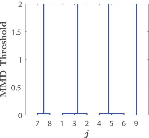
First let us apply the randomly generated control signals and () in Example 7 to all 9 linear ensembles. Then, we take the collections of calibrated aggregated measurements as , , where and are the th-order moment trajectory of under the control inputs and the null-inputs , respectively. The pairwise MMDs among all 9 ensembles are presented in Table VI. Figure 7 presents the agglomerative hierarchical cluster tree of the 9 ensembles, based on the pairwise MMDs in Table VI. It is shown in Figure 7 that the linear ensembles are clustered into clusters, namely , , and , where the ensembles in each cluster have the same dynamics.
V Conclusions
In this paper, we propose a novel framework to learn the system dynamics of an unknown ensemble using its aggregated measurements in reproducing kernel Hilbert spaces. We demonstrate that we can identify unknown ensembles by comparing the distribution of their aggregated measurements after perturbing the systems using random control inputs. Additionally, by introducing a new notion of aggregated Markov parameters, we also provide a systematic approach to recognize and cluster unknown ensembles by linear approximation, without the need of a baseline model or any prior knowledge on the system dynamics. Ample examples are included in the paper to illustrate the efficacy and robustness of our framework.
Appendix
In this appendix, we review some technical results regarding RKHS and universal kernels that are necessary to the development of our framework.
Definition 5.
Let be a compact metric space. A continuous kernel is said to be universal if the RKHS associated with is dense in with respect to sup-norm, i.e., for every and , there exists such that .
Theorem 3.
Let be a compact metric space, be a separable Hilbert space, and be an injective map. Then, the Gaussian-RBF-type kernel , given by
| (13) |
is a universal kernel, where and denotes the norm induced by inner product of .
Proof.
See [4], Theorem 2.2. ∎
Lemma 4.
Let be a non-empty set, be a reproducing kernel, and be its associated RKHS. Given a probability distribution defined on , if is measurable and , then the kernel mean embedding of , denoted as , is in , i.e.,
Proof.
See Lemma 3 in [8]. ∎
Lemma 5.
Let be compact, , , and . The infinite sequence , where
is square-summable, i.e., , . Furthermore, it holds that
Proof.
It suffices to show that . This is evident since
where , , and are the element-wise absolute values of , , and , respectively; and the second inequality holds since is continuous.
To show that , it suffices to observe that
where denotes the sup-norm over and is the Lebesgue measure of . ∎
Lemma 6.
Let be a random variable. If the limit exists, then the moment generating function of , denoted as , has a power series expansion over the whole real line, i.e.
for all .
Proof.
It is not hard to observe that the power series has a radius of convergence, denoted as , such that
| (14) |
Let . Then, (14) is computed as
| (15) |
By Stirling’s formula, when is sufficiently large. Hence as , which implies that . Therefore, the power series converges for all . ∎
References
- [1] Aaron Becker and Timothy Bretl. Approximate steering of a unicycle under bounded model perturbation using ensemble control. IEEE Transactions on Robotics, 28(3):580–591, 2012.
- [2] Eric Brown, Jeff Moehlis, and Philip Holmes. On the phase reduction and response dynamics of neural oscillator populations. Neural Computation, 16(4):673–715, 2004.
- [3] Xudong Chen. Structure theory for ensemble controllability, observability, and duality. Mathematics of Control, Signals, and Systems, 31:1–40, 2019.
- [4] Andreas Christmann and Ingo Steinwart. Universal kernels on non-standard input spaces. In J. Lafferty, C. Williams, J. Shawe-Taylor, R. Zemel, and A. Culotta, editors, Advances in Neural Information Processing Systems, volume 23, pages 406–414. Curran Associates, Inc., 2010.
- [5] Corinna Cortes, Mehryar Mohri, Michael Riley, and Afshin Rostamizadeh. Sample selection bias correction theory. In Yoav Freund, László Györfi, György Turán, and Thomas Zeugmann, editors, Algorithmic Learning Theory, pages 38–53. Springer Berlin Heidelberg, 2008.
- [6] Gunther Dirr and Michael Schönlein. Uniform and -ensemble reachability of parameter-dependent linear systems, 2018. arXiv:1810.09117 [math.OC].
- [7] Steffen J Glaser, T Schulte-Herbrüggen, M Sieveking, O Schedletzky, Niels Christian Nielsen, Ole Winneche Sørensen, and C Griesinger. Unitary control in quantum ensembles: Maximizing signal intensity in coherent spectroscopy. Science, 280(5362):421–424, 1998.
- [8] Arthur Gretton, Karsten M. Borgwardt, Malte J. Rasch, Bernhard Schölkopf, and Alexander Smola. A kernel two-sample test. Journal of Machine Learning Research, 13(25):723–773, 2012.
- [9] Uwe Helmke and Michael Schönlein. Uniform ensemble controllability for one-parameter families of time-invariant linear systems. Systems & Control Letters, 71:69 – 77, 2014.
- [10] Wassily Hoeffding. Probability inequalities for sums of bounded random variables. In The Collected Works of Wassily Hoeffding, pages 409–426. Springer, 1994.
- [11] MohammadMehdi Kafashan and ShiNung Ching. Optimal stimulus scheduling for active estimation of evoked brain networks. Journal of Neural Engineering, 12(6):066011, Oct 2015.
- [12] George Kimeldorf and Grace Wahba. Some results on tchebycheffian spline functions. Journal of Mathematical Analysis and Applications, 33(1):82–95, 1971.
- [13] Karsten Kuritz, Shen Zeng, and Frank Allgöwer. Ensemble controllability of cellular oscillators. IEEE Control Systems Letters, 3(2):296–301, 2018.
- [14] Jr-Shin Li. Ensemble control of finite-dimensional time-varying linear systems. IEEE Transactions on Automatic Control, 56(2):345–357, 2011.
- [15] Jr-Shin Li, Isuru Dasanayake, and Justin Ruths. Control and synchronization of neuron ensembles. IEEE Transactions on Automatic Control, 58(8):1919–1930, 2013.
- [16] Jr-Shin Li, Justin Ruths, Tsyr-Yan Yu, Haribabu Arthanari, and Gerhard Wagner. Optimal pulse design in quantum control: A unified computational method. Proceedings of the National Academy of Sciences, 2011.
- [17] Jr-Shin Li, Wei Zhang, and Lin Tie. On separating points for ensemble controllability. SIAM Journal on Control and Optimization, 58(5):2740–2764, 2020.
- [18] Wei Miao, Gong Cheng, and Jr-Shin Li. On numerical examination of uniform ensemble controllability for linear ensemble systems. IEEE Control Systems Letters, 5(6):1898–1903, 2020.
- [19] Wei Miao and Jr-Shin Li. A convex-geometric approach to ensemble control analysis and design in a hilbert space, 2020. arXiv:2003.09987 [math.OC].
- [20] Wei Miao and Jr-Shin Li. A geometric approach to linear ensemble control analysis and design. In 2020 American Control Conference (ACC), pages 4600–4605. IEEE, 2020.
- [21] Michael G Rosenblum and Arkady S Pikovsky. Controlling synchronization in an ensemble of globally coupled oscillators. Physical Review Letters, 92(11):114102, 2004.
- [22] Michael Schönlein and Uwe Helmke. Controllability of ensembles of linear dynamical systems. Mathematics and Computers in Simulation, 125:3 – 14, 2016.
- [23] Paulo Tabuada and Bahman Gharesifard. Universal approximation power of deep neural networks via nonlinear control theory. arXiv preprint arXiv:2007.06007, 2020.
- [24] Lin Tie, Wei Zhang, Shen Zeng, and Jr-Shin Li. Explicit input signal design for stable linear ensemble systems. IFAC-PapersOnLine, 50(1):3051–3056, 2017. 20th IFAC World Congress.
- [25] Shuo Wang and Jr-Shin Li. Fixed-endpoint optimal control of bilinear ensemble systems. SIAM Journal on Control and Optimization, 55(5):3039–3065, 2017.
- [26] Shuo Wang and Jr-Shin Li. Free-endpoint optimal control of inhomogeneous bilinear ensemble systems. Automatica, 95:306 – 315, 2018.
- [27] E Weinan. A proposal on machine learning via dynamical systems. Communications in Mathematics and Statistics, 5(1):1–11, 2017.
- [28] Shen Zeng and Frank Allgoewer. A moment-based approach to ensemble controllability of linear systems. Systems & Control Letters, 98:49–56, 2016.
- [29] Shen Zeng, Hideaki Ishii, and Frank Allgöwer. Sampled observability and state estimation of linear discrete ensembles. IEEE Transactions on Automatic Control, 62(5):2406–2418, 2017.
- [30] Shen Zeng, Wei Zhang, and Jr-Shin Li. On the computation of control inputs for linear ensembles. In 2018 Annual American Control Conference (ACC), pages 6101–6107. IEEE, 2018.
- [31] Anatoly Zlotnik and Jr-Shin Li. Synthesis of optimal ensemble controls for linear systems using the singular value decomposition. In 2012 American Control Conference (ACC), pages 5849–5854, June 2012.
- [32] Anatoly Zlotnik, Raphael Nagao, István Z Kiss, and Jr-Shin Li. Phase-selective entrainment of nonlinear oscillator ensembles. Nature Communications, 7(1):1–7, 2016.