Multi-Band Wi-Fi Sensing with Matched Feature Granularity
Abstract
Complementary to the fine-grained channel state information (CSI) and coarse-grained received signal strength indicator (RSSI) measurements, the mid-grained spatial beam attributes (e.g., beam SNR) during the millimeter-wave (mmWave) beam training phase were recently repurposed for Wi-Fi sensing applications such as human activity recognition and indoor localization. This paper proposes a multi-band Wi-Fi sensing framework to fuse features from both CSI at sub-7 GHz bands and the mid-grained beam SNR at 60 GHz with feature granularity matching that pairs feature maps from the CSI and beam SNR at different granularity levels with learnable weights. To address the issue of limited labeled training data, we propose to pre-train an autoencoder-based multi-band Wi-Fi fusion network in an unsupervised fashion. For specific sensing tasks, separate sensing heads can be attached to the pre-trained fusion network with fine-tuning. The proposed framework is thoroughly validated by three in-house experimental datasets: 1) pose recognition; 2) occupancy sensing; and 3) indoor localization. Comparison to a list of baseline methods demonstrates the effectiveness of granularity matching. Ablation study is performed as a function of the number of labeled data, latent space dimension, and fine-tuning learning rates.
Index Terms:
Wi-Fi sensing, WLAN sensing, channel state information, beam attributes, fusion, autoencoder, millimeter wave, fingerprinting, deep learning.I Introduction
Wi-Fi sensing or WLAN sensing has received tremendous attention over the past decade. More recently (September 2020), IEEE Standards Association established a new task group for WLAN sensing for making greater use of technologies towards new industrial and commercial applications in home security, entertainment, energy management (HVAC, light, device power savings), elderly care, and assisted living [1, 2].
Most Wi-Fi sensing frameworks use either fine-grained channel state information (CSI) [3, 4, 5, 6, 7, 8, 9, 10, 11, 12] or coarse-grained RSSI measurements [13, 14, 15, 16, 17, 18, 19, 20, 21, 22, 23, 24, 25, 26, 27, 28, 29]; see more detailed literature review in the next section. The conventional RSSI measurement suffers from the measurement instability and coarse granularity of the channel information, leading to limited accuracy for localization. The CSI measurement is more fine-grained but requires access to physical-layer interfaces and high computational power to process a large amount of sub-carrier data.
These limitations motivate a recent adoption of mid-grained intermediate channel measurements which are more informative (e.g., in the spatial domain) than the RSSI measurement and easier to access than the lower-level CSI measurement [30, 31, 32, 33, 34]. Specifically, spatial beam SNRs that are inherently available (with zero overhead) for beam training for IEEE 802.11ad/ay standards operating at millimeter-wave (mmWave) bands [35, 36, 37], are used to construct the fingerprinting/training dataset. The use of the mid-grained channel measurement was made possible by earlier efforts in [38, 39, 40] which enabled easy access to beam SNR measurements from commercial off-the-shelf (COTS) 802.11ad Wi-Fi routers.
Fusion-based approaches have been considered before to improve robustness and accuracy. Most fusion-based localization methods make use of heterogeneous sensor modalities such as on-device or wearable sensors, e.g., inertial navigation system (INS), magnetic sensors, accelerometer, ultrasound, and other surrounding sensors such as camera, Bluetooth, and ZigBee. These heterogeneous sensor signals are then fused with Wi-Fi signals (either RSSI or CSI) in the traditional maximum likelihood framework or more advanced deep learning context. For instance, continuous localization of indoor pedestrians was achieved using INS with tracking errors adjusted by the Wi-Fi [41]. DeepFusion combines heterogeneous wearable (e.g., smartphone and smartwatch) and wireless (Wi-Fi and acoustic) sensors for human activity recognition [42]. A recent survey paper can be found in [43].
When only wireless radio frequency (RF) sensors (e.g., Wi-Fi, Bluetooth, ZigBee, LTE) are considered, the fusion of the coarse-grained RSSI, Bluetooth, and ZigBee measurements was considered in [44] with the nearest neighbor (NN) method. In [45], the fine-grained CSI was used first to extract the Angle-of-Arrival (AoA) measurements and then fused with RSSI from Bluetooth in the context of the traditional maximum-likelihood estimation (MLE) framework.
If we further narrow down the scope to Wi-Fi-only measurements, the fusion between the CSI and RSSI can be done in a way similar to [45] or in a straightforward manner by concatenating the scalar RSSI to the high-dimension CSI. For the CSI Wi-Fi measurements, [46] proposed to fuse the phase and amplitude of the fine-grained CSI, as opposed to the magnitude-only CSI, for the purpose of localization. When multiple access points (APs) are available, the fusion of multi-view CSI measurements over APs was considered in [47] using the generalized inter-view and intra-view discriminant correlation analysis. [48] proposed to fuse the probability maps from multiple APs and multiple transmit antennas. Moreover, [49] propose the Maximum Mean Discrepancy (MMD) as a transfer learning technique for indoor localization with different placement of the APs.


In this paper, we propose to fuse the fine-grained CSI measurements at sub-6 GHz from multiple spatial streams and the mid-grained beam SNRs at the mmWave band of 60 GHz. Both kinds of Wi-Fi channel measurements provide rich yet complementary features in different physical domains. As complex-valued amplitudes at OFDM subcarrier tones, the CSI measurements are equivalent to the power delay profile (PDP) in the time domain and reflect the power distribution along propagation paths. On the other hand, the beam SNRs are more about spatial-domain channel measurements over various beamforming directions or beamspace. In particular, our contributions and results are summarized as follows:
- •
First work to fuse the two distinct kinds of Wi-Fi channel measurements at different frequency bands. The mid-grained beam SNRs are richer and more stable channel measurements than the coarse-grained RSSI and can lead to more meaningful fusion with the fine-grained CSI.
- •
Introduce a multi-band Wi-Fi fusion method that accounts for the granularity matching between the CSI and beam SNR measurements. The granularity matching is realized via a learnable fusion block that pairs any two feature maps from the CSI and beam SNR at different feature levels and assigns adaptive weights to the paired feature maps.
- •
Propose an autoencoder-based multi-band fusion network that can be pre-trained in an unsupervised fashion. With the pre-trained fusion network, we propose attaching multi-task heads to the fused features by fine-tuning the fusion block and training the multi-task heads from the scratch.
- •
Implement an in-house multi-band Wi-Fi testbed consisting of commercial ac- and ad-compliant Wi-Fi routers and collect real-world measurements in standard room environments (e.g., apartment and lab) for three Wi-Fi sensing tasks: 1) pose recognition, 2) occupancy sensing, and 3) indoor localization.
- •
Conduct comprehensive performance analysis by including four baseline methods and evaluating performance as a function of the number of labeled training data, latent space, and the fine-tuning learning rates.
II Wi-Fi Channel Measurements: An Overview
In the following, we provide a literature review on Wi-Fi channel measurements and their applications in indoor localization, human activity recognition, and wireless sensing.


II-A RSSI: Received Signal Strength Indicator
In a typical indoor environment, the baseband signal voltage at an RF receiver at a given time is measured as [50]
| (1) |
where and are the amplitude and phase of the -th multipath component, and is the total number of multipath components.; see Fig. 1 (a) and (b) for an illustration. Then RSSI is the received power in decibels (dB) as
| (2) |
Early Wi-Fi based indoor localization systems used RSSI measurements to estimate indoor location in a direct localization fashion [13, 14, 15, 16]. For fingerprinting-based methods, RSSI was used directly as fingerprinting data in systems such as Radar [17], Compass [18], and Horus [19] due to easy access to 802.11ac- and 802.11n-compliant devices. Classical machine learning methods, e.g., the -nearest neighbor (NN) and support vector machine (SVM), and probabilistic Bayesian methods have been applied to RSSI fingerprinting measurements [17, 20, 21, 24, 19, 26, 25, 22, 23]. Advanced deep learning methods such as multi-layer neural networks [28] and recurrent neural networks (RNNs) [29] showed improved localization performance over classical machine learning approaches.
II-B CSI: Channel State Information
By modeling the wireless channel as a temporal linear filter, one can measure the channel impulse response (CIR) as
| (3) |
where is the delay of the -th multipath, and is the Dirac delta function. In other words, the channel can be represented by the multipath amplitude and phase distribution at corresponding delays; see the middle figure of Fig. 1 (c) for an illustration. Given the CIR , the received signal is the temporal convolution of the preamble and : . The channel frequency response (CFR) or, equivalently, the Fourier transform of the CIR, is often measured as
| (4) |
where is the Fourier transform of and is the complex conjugate of the Fourier transform of . In commercial Wi-Fi devices, a group of sampled CFRs at a list of subcarriers are measured as
| (5) |
where is the -th subcarrier frequency; see the bottom figure of Fig. 1 (c) for an illustration. These complex-valued CFRs are reported to upper network layers in the format of CSI [51]. Compared with the coarse-grained RSSI, the CSI provides a fine-grained channel measurement with better capability to resolve multipath in the time or frequency domain. While still suffering from temporal fluctuation, the CSI provides a set of complex-valued random variables (i.e., multipath components) compared with the scalar RSSI.
Recent efforts on CSI extraction from COTS Wi-Fi devices, e.g., Intel Wi-Fi Link radio [52], Atheros n chipsets [53], and Cypress ac chipsets [54], have enabled access to the CSI over a bandwidth of up to MHz at sub- GHz (i.e., and GHz bands). This has sparked a large swath of learning-based Wi-Fi sensing applications [3, 4, 5, 6, 7, 8, 55, 56, 57, 58, 59, 60, 61, 62, 63, 64, 65]. For instance, ConFi [9] used convolutional neural networks (CNNs) to train CSI measurements from three antennas, to classify the location and estimate location coordinates. [10] fingerprinted full CSI over multiple time instants, calibrated their phases, and fitted one autoencoder for one location. CSI measurements can also be directly trained to regress the coordinate [11, 12]. More recently, [63] used annotations from camera images to train fine-grained CSI measurements for pose and human tracking.
II-C Beam SNR: mmWave Beam Training Measurement
At mmWave bands, another type of channel measurements from the mandatory beam training phase provides a mid-grained measurement in the beam angle domain for Wi-Fi sensing. During the mandatory beam training phase defined by the ad/ay standards, directional probing beampatterns are used to determine desired directions for subsequent data communication to compensate large path loss at mmWave bands [35, 36, 37]. For each probing beampattern (also referred to as beam sectors), beam SNR is computed as a measure of beam quality.
For a given pair of transmitting and receiving beampatterns, corresponding beam SNR can be defined as
| (6) |
where is the index of beampattern, and are the transmitting and receiving azimuth angles for the th path, respectively, is the signal power at the th path, and are the transmitting and receiving beampattern gains at the th path for the th beampattern, respectively, and is the noise variance. Fig. 2 (a) shows an example of paths between the transmitting side that probes the spatial domain using a directional beampattern and the receiving side which is in a listening mode with a quasi-omni-directional beampattern, while Fig. 2 (c) shows a number of pre-determined beampatterns used at the transmitting side to compute corresponding beam SNRs. Due to antenna housing and hardware impairments, these beampatterns exhibit fairly irregular shapes at the GHz band [38, 39].
II-D CSI versus Beam SNR
By comparing Fig. 1 (a) with Fig. 2 (a), several observations can be made between the CSI and beam SNR. First, multipath propagation is richer at sub- GHz bands (i.e., paths) than GHz bands (i.e., paths). Second, the through-wall path (denoted as dotted lines) in Fig. 1 (a) does not survive in the GHz link due to its much shorter wavelength and less capability to penetrate obstacles (e.g., wall). Third, mmWave Wi-Fi devices are equipped with a phased array that enables highly directional beampatterns while antenna elements of sub- GHz Wi-Fi devices are mostly in an omni-directional mode. Although multiple antenna elements at sub- GHz can be used for beamforming, the beampatterns are less directional than the mmWave Wi-Fi device due to the smaller number of antennas and the relatively large inter-element spacing. Consequently, these two distinct kinds of Wi-Fi channel measurements probe the scene with different lenses and may exhibit complementary channel features in different physical space (time/frequency versus space) and domains (omni-directional antennas versus directional beampatterns).
III Multi-Band Wi-Fi Sensing with Supervised Learning
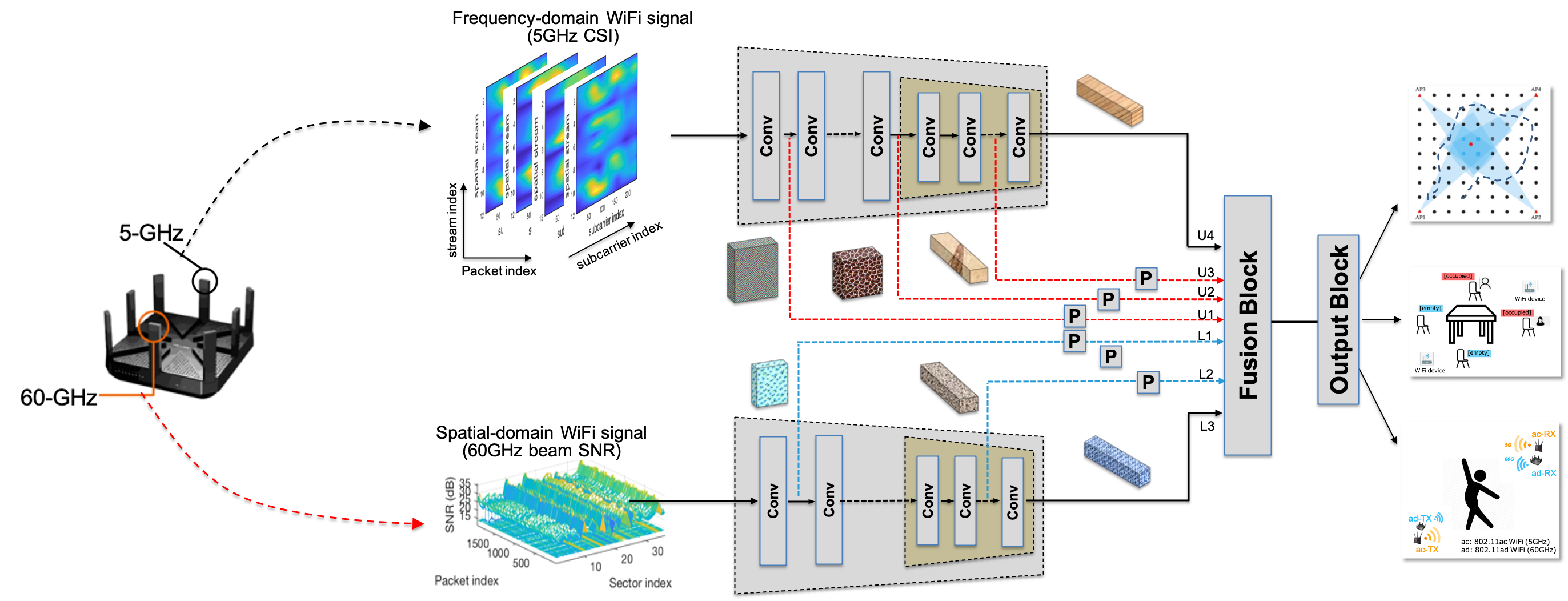
In this section, we introduce the multi-band Wi-Fi fusion framework that combines the features from both the fine-grained CSI measurements and the mid-grained beam SNRs. Particularly, we account for the feature granularity by designing a learnable granularity matching network that pairs multi-scale features from the CSI and beam SNR and assigns linear weights to the paired features. Specifically, Fig. 3 shows the multi-band Wi-Fi sensing network that consists of three blocks: 1) feature extraction, 2) feature fusion with granularity matching, and 3) separate output blocks for individual sensing tasks. Such a framework is then trained end-to-end for human activity recognition, occupancy detection, and localization tasks, respectively, in a supervised fashion. In the following, we introduce each block in more detail.
III-A Preliminary
Like traditional fingerprinting-based Wi-Fi sensing methods, we follow the standard procedure by collecting both CSI and beam SNR measurements corresponding to each class (e.g., pose, occupancy pattern, and location/orientation) as the fingerprinting data. Specifically, we use and to denote the CSI measurements from spatial streams over subcarriers and the beam SNRs from beampatterns. For a given class , fingerprinting snapshots, and , are collected to construct the offline training dataset. By collecting many realizations of both Wi-Fi channel measurements at classes, we will have sets of training data in the training dataset. For the labeled data, the label class is automatically attached to both and .
III-B Feature Extraction
In Fig. 3, the feature extraction block employs two separate convolution networks to encode the feature maps for CSI-only and beam SNR-only measurements. Specifically,
| (7) |
where , , and denotes the convolution operation (including batch normalization, pooling and activation functions) for CSI-only and beam SNR-only feature extraction with kernel parameters at the -th layer. Overall, we use and convolution layers for, respectively, the CSI and beam SNRs to gradually shrink the dimension of the feature maps while increasing the number of feature maps. The -th feature map is denoted as , where are, respectively, the number of channels, height and width of the -th feature map. Note that the number of layers for CSI can be different from that for beam SNRs, i.e., .

To be more specific, we use convolutional blocks, respectively, for the CSI and beam SNR encoders, as shown in Fig. 4. Each convolution block consists of a standard convolution layer followed by a batch normalization layer and a rectified linear unit (ReLU) activation layer. For the CSI encoder, we use the first convolution blocks and maxpooling layers to increase the number of feature maps to and downsize the dimension to . Similarly, the beam SNR encoder uses convolution blocks to downsize the input to the same feature space. Then the subsequent convolution blocks share the same structure as highlighted in tan colored blocks of Fig. 4.
III-C Feature Fusion
Since the CSI and beam SNRs are two distinct Wi-Fi channel measurements with different channel feature granularities, one needs to take into account the granularity correspondence for the multi-band Wi-Fi fusion. For instance, CSI features at later convolution layers may have a better correspondence to beam SNR features at earlier layers as the CSI is likely to have finer granularity than the beam SNR. To this end, we extract multi-scale feature maps at selected convolution layers as two sets of threads
| (8) |
where and denote the selected layer indices of the CSI and, respectively, beam SNR encoders. For instance of Fig. 3, we have layer indices in and elements in .
With an identity mapping or aa linear projection to a smaller dimension, the features from the upper encoder branch are mapped to and the lower ones as in Fig. 3, where denoting the cardinality of the set . To find correspondences between the extracted multi-scale features from the CSI and beam SNR, the proposed fusion scheme concatenates two selected feature maps from the two encoders: one is from the CSI encoder and the other from the beam SNR encoder.
| (9) |
where denotes the fusion pair index with . For instance, we have pairs in Fig. 5 by pairing one of four CSI features and one of three beam SNR features .
Then, each concatenated feature is fused with a fully connected layer into the same latent dimension ,
| (10) |
where is the projection weight matrix for the -th pair with denoting the bias term. The final fusion layer is a linear combination of the fused feature map as
| (11) |
where is the fusion weight that can be learned from the training data. The fusion weights acts as a soft selection vector on all concatenated feature vectors. A higher weight implies that the corresponding pair of features has a better granularity matching level. In the case of and , the fused feature map (11) only combines the features at the final layers of the two encoders. In contrast, with non-zero , the proposed fusion scheme allows multi-scale features from earlier layers to find its correspondence from the other branch and contribute to the final fused features.

III-D Output Block
In Fig. 3, the fused feature map is fed into the output block to generate the output vector . The output block consists of a number of fully-connected layers:
| (12) |
where , , and with and denoting the activation function such as ReLU for and an identity mapping when at the final output layer.
III-E Cost Function
To train the multi-band Wi-Fi sensing network with labeled training data with the label , corresponding output of the last layer is first normalized with the softmax operation as
| (13) |
where is the th element of the normalized output . Then, the cross-entropy loss function is computed over the score vector and the corresponding one-hot label vector as
| (14) |
where the one-hot label vector is at the -th element and elsewhere. Note that, for different sensing applications, the dimension of the output vector may be different, depending on the number of classes. For instance, for the pose recognition and occupancy sensing and for the indoor localization.

IV Multi-Band Wi-Fi Sensing with Transfer Learning
Although it is simple to train the above network separately for each sensing task, the offline fingerprinting phase is time- and manpower-consuming [66, 67]. To label the data, one has to associate both channel measurements with the ground-truth labels, in the form of pose gesture, occupancy pattern, or user location. This issue is severe when one needs to build up the training dataset when the number of classes is large. Even worse, after a Wi-Fi sensing system is deployed, the ground-truth information is hard to obtain, while the Wi-Fi devices can still gather or “listen” the environment and access to multi-band Wi-Fi channel measurements.
To meet the challenges of limited labeled training data, we consider an unsupervised fusion approach using a multi-stream autoencoder to train the encoder and fusion blocks with unlabeled training data and with , possibly pooled from multiple sensing tasks. With the unsupervised trained encoder and fusion blocks, a transfer learning approach is then applied to fine-tune the fusion block and retrain a new attached output block for individual sensing task with limited labeled data and .
IV-A Unsupervised Multi-Stream Autoencoder with Feature Granularity Matching
Fig. 6 shows a multi-stream autoencoder architecture that uses the same two-branch encoder as in the previous section to extract the features of the two Wi-Fi channel measurements, the same fusion block taking multi-scale features from the two encoder branches and matching the feature granularity, and a new two-branch decoder to synthesize the two input Wi-Fi channel measurements from the same fused feature at the output of the fusion block.
The multi-stream autoencoder can be trained end-to-end using unlabeled (“listening”) multi-band Wi-Fi data that can be pooled from multiple sensing tasks. The motivation here is that, without any class label, one can still train or update the feature extractor and fusion blocks continuously at local Wi-Fi devices or edge units. Whenever new labeled data are available (e.g., users share their location sporadically), the limited amount of labeled data can be used to train the output block for the task-specific sensing task while leaving the training of feature extraction and fusion blocks to the unlabeled data. In the following, we elaborate on each building block of Fig. 6.
IV-A1 Encoder
At the encoder side, we re-use the same two encoder networks to extract the feature maps for CSI and beam SNR measurements in Fig. 4. Multi-scale features from multiple levels of both encoder branches are extracted as for the feature fusion with granularity matching.
IV-A2 Fusion
IV-A3 Decoder
At the decoder side, the fused feature is fed to two separate decoders to recover the input CSI and beam SNR measurements simultaneously. Particularly,
| (15) |
where is the output of the fusion block in Fig. 6 that is simultaneously fed into the two decoders, denotes the transposed convolution or upsampling operation at the -th layer of the two decoders with corresponding parameters . Usually, we implement the decode network with a mirrored architecture of its encoder network. Therefore, we keep the same number of layers, and , in the decoders. The decoder architectures for the beam SNR and CSI mirror their corresponding encoder architectures in Fig. 4.
IV-A4 Cost Function
To train the autoencoder-based fusion network with unlabeled data, we adopt a weighted mean-squared error (MSE) as the cost function:
| (16) |
where and are the CSI and beam SNR training samples, are corresponding outputs of the two decoders, and is the hyperparameter to balance the reconstruction error between the CSI and beam SNR branches.
IV-B Transfer Learning with Limited Labeled Data
Once the autoencoder-based multi-band Wi-Fi fusion network in Fig. 6 is trained, we use the transfer learning to freeze the encoder parameters, fine-tune the fusion block, remove the decoder block, and attach a new output classification block for each sensing task, as shown in Fig. 7.
With the labeled training data for each sensing task, we retrain the output block which takes the same form of (12) and outputs the vector . Specifically, the transfer learning computes the classification cost function of (14) and back-propagates the gradient of the cost function with respect to the parameters in the output block in a large step size, e.g., a learning rate of , while fine-tuning the parameters within the fusion block with a small training step size (e.g., a learning rate of or smaller) on the linear fusion weights of (11) and an even smaller learning rate on of (III-B). It is worth noting that, for each sensing task, the transfer learning needs to apply separately to train separate output blocks. Once the entire network of Fig. 7 is re-trained, we deploy the network with test datasets for different sensing tasks.

V Performance Evaluation
In the following, we present the performance evaluation for the proposed multi-band Wi-Fi fusion using real-world experimental datasets for three sensing tasks: 1) pose recognition; 2) occupancy sensing; and 3) indoor localization. For each of these three tasks, we compare the proposed fusion methods with the CSI-only and beam SNR-only methods.
V-A Experiment Setup
The data collection system consists of multiple commercial ac- and ad-compliant routers and devices in a configuration shown in Fig. 8 (a)-(c) for the three sensing tasks. Both 5 GHz CSI and 60 GHz beam SNR measurements are recorded in the routers and sent to a workstation via Ethernet cables. The data collection system is deployed in standard indoor room settings, as shown in Fig. 8 (d)-(f).
CSI from 802.11ac devices: We use ASUS RT-AC86U routers with external and internal antennas to extract the CSI measurements at GHz and modified its firmware using the Nexmon CSI Extractor Tool of [54]. It allows per-frame CSI extraction for up to spatial streams using all four receive chains on Broadcom and Cypress Wi-Fi chips with up to 80 MHz bandwidth in both the 2.4 and 5 GHz bands. It also supports devices such as the low-cost Raspberry Pi platform and mobile platforms such as Nexus smartphones. Other CSI tools are also available at GHz and GHz [52, 53], but none of them supports MHz wide channels within the newer ac standard (with respect to n/g). In addition, it supports various Tx-Rx antenna configurations, up to MIMO. In our in-house testbed, we use a pair of ASUS routers to record all spatial streams over subcarriers. However, to mimic a standard mobile terminal, we only use spatial streams which are equivalent to a configuration of using ASUS routers with external antennas and mobile user with a single antenna.
Beam SNR from 802.11ad devices: We use TP-Link Talon AD7200 routers to collect beam SNRs at GHz. Complying with IEEE 802.11ad standards, this router implements Qualcomm QCA9500 transceiver that supports a single stream communication in GHz range using analog beamforming over -element planar array. The raw beam SNRs are extracted by using the open-source software package in [68]. By matching the patterns of IEEE ad beam training frames with the memory inside the chip, one can identify parts of the firmware handling the beam training frames and extract beam SNR measurements from these memory addresses. For Talon AD7200 routers, the beam SNR measurements are further quantized in a stepsize of dB. Overall, from one beam training, one AP can collect beam SNRs for transmitting beampatterns. It is noted that the resulting beampatterns depart from the theoretical ones and exhibit fairly irregular shapes due to hardware imperfections and housing at GHz.


V-B Sensing Tasks and Datasets
With the above multi-band Wi-Fi testbed, we conducted multiple sensing tasks as follows:
V-B1 Pose Recognition
Fig. 8 (a) shows the experimental configuration for the pose recognition by using one Wi-Fi station (including both ac and ad routers) in the front of the subject and one station behind the subject. Both stations are placed on a stand of a height of meters with a distance of approximately meters. As shown in Fig. 8 (d), the subject is asked to perform a total of poses including distinct gestures like ‘sit’, ‘stand with left arm lifted’, ‘stand with both arms lifted’, etc. For each pose, we recorded independent sessions with different time durations and with sufficient time separation in between consecutive two sessions. We grouped the measurements in the first four data sessions as the training data and those in the last three sessions as the test data for the maximum time separation. The numbers of both CSI and beam SNR samples (in brackets) in the training and test datasets are listed in the second and third columns of Table I.
V-B2 Occupancy Sensing
Fig. 8 (b) shows the experimental configuration for occupancy sensing around a table in a small living room environment. Two stations are placed in the top left and bottom right corners in a diagonal configuration. The selected occupancy patterns cover both a single subject sitting on one of the four chairs and two subjects, as shown in Fig. 8 (e). During the data collection, the subject is free to move body parts such as typing the laptop and reading the paper as long as the subject is fixed at the location. We also recorded independent sessions with sufficient time separation in between consecutive two sessions and grouped the measurements as the training and test datasets in the same way as the pose recognition task. The numbers of both CSI and beam SNR samples (in brackets) in the training and test datasets are listed in the fourth and fifth columns of Table I. Similar data augmentation is performed to align the beam SNR samples with the higher density CSI data in the training dataset.
V-B3 Indoor Localization
Finally, we consider indoor localization in a standard lab environment with multiple AP stations (including one ac and three ad routers) and one user on the grid, as denoted by blue dots in Fig. 8 (f). The AP stations are placed around the three corners of the fingerprinting area, denoted as triangles in Fig. 8 (c). The number of grids is with a grid size of cm. For each grid, we place another station with both ac and ad devices acting as a single-antenna mobile user and record multiple data sessions for training and independent testing.
V-C Wi-Fi Signal Preprocessing
For the fingerprinting dataset, we perform preprocessing steps to calibrate CSI and beam SNR measurements. For the CSI measurements from commercial routers (ASUS RT-ACU in our case), known hardware issues include [53, 69, 70, 71, 72]
- 1.
Power control uncertainty: The raw CSI amplitude is compensated by the automatic gain controller (AGC) and mixed with a power amplifier uncertainty error, causing an amplitude offset;
- 2.
Sample frequency offset (SFO): the sampling frequencies between the transmitter and receiver also exhibit an offset due to non-synchronized clocks, causing a time shift to the digitally sampled signal after the analog-to-digital converter (ADC);
- 3.
Package boundary detection (PBD) error: due to correlator sensitivity of packet detector, the packet detection at the receiver introduces another time shift, resulting in a random phase offset to the raw CSI;
- 4.
Carrier frequency offset (CFO): The carrier frequencies between the transmitter and receiver cannot be perfectly synchronized. The CFO is initially compensated by a CFO corrector at the receiver. However, the compensation is incomplete due to the hardware imperfection, leaving residual CFO and leading to a phase offset over time;
- 5.
Phase offsets between RF chains: The CSI phases at different RF chains are not synchronized perfectly and it results in semi-deterministic phase offsets between RF chains;
result in both amplitude and phase distortions to raw CSI measurements.
For Item 1), the CSI amplitude offsets in individual bands can be removed by an averaging or a standardization operation [53]; see Fig.9 (a) and (b). For Items 2)-4), the phase offset over subcarriers and/or packets can be calibrated by either a linear phase fitting approach used in the SpotFi [69, Algorithm 1] or a multi-subband phase correction approach in [53, 70]. The compensated phases (with respect to the first subcarrier) of multiple packets are stable over time, as shown in Fig.9 (c) and (d). The combined amplitude and phase compensated CSI can serve as an indirect measurement of the time-of-flight (ToF) or delay power profile of the multi-path propagation.
To further extract the angle (e.g., AoA) information across multiple antennas, one may need to compensate the initial phase offsets (of the phased-locked loops (PLLs)) between RF chains of Item 5) by connecting a coaxial cable between the transmitter and receiver [72]. However, due to the semi-deterministic nature of this phase offset and the fixed amount of phase permutations ( phase permutations for antennas), we skip this antenna calibration and treat the raw CSI across antennas as augmented CSI data. Moreover, we remove guard subcarriers as corresponding amplitudes are always zeros.
On the other hand, we found that the beam SNRs as positive scalar values (so no need for the phase calibration) are much more consistent than the CSI measurement, except for a scaling effect over multiple packets; see Fig. 9 (e). As a result, the raw beam SNRs in the training data are augmented by multiplying them with a random scaling factor in and then standardized over each beam index.


| Class ID | Training-Pose | Test-Pose | Training-Occ. | Test-Occ.) |
|---|---|---|---|---|
| 0 | 434 (6510) | 151 | 508 (7620) | 230 |
| 1 | 499 (7485) | 149 | 717 (10755) | 290 |
| 2 | 325 (4875) | 173 | 438 (6570) | 189 |
| 3 | 347 (5205) | 129 | 483 (7245) | 184 |
| 4 | 238 (3570) | 88 | 602 (9030) | 235 |
| 5 | 314 (4710) | 96 | 815 (12225) | 217 |
| 6 | 272 (4080) | 119 | 535 (8025) | 200 |
| 7 | 432 (6480) | 135 | 608 (9120) | 271 |
V-D Baseline Methods
For a fair comparison, we consider a list of baseline methods with the proposed fusion network with granularity matching (GM) for both supervised learning and transfer learning:
- •
CSI-Only uses only the fine-grained CSI measurements as the input. The neural network follows the same architecture of the upper CSI encoder of Fig. 3 for supervised learning and the upper CSI branch (both encoder and decoder) of Fig. 6 for unsupervised fusion. The only difference is that the input is only the CSI and we only change the first convolutional layer configuration to reflect the change in the input dimension while keeping all other layers the same.
- •
- •
- •
For performance evaluation, we use the confusion matrix as the criterion:
| (17) |
where and are indices, respectively, for the estimated and true labels, and is the number of samples in the test dataset for the index . In addition, is the estimate by using the th sample batch from the test data collected at the th label.
| CSI | bSNR | IF | FF | GM | |
| All-Pose | 74.8% | 92.3% | 89.5% | 90.0% | 94.4% |
| 40% | 64.0% | 86.8% | 84.2% | 83.0% | 90.2% |
| 20% | 57.1% | 81.8% | 83.2% | 79.9% | 89.9% |
| 10% | 48.7% | 77.9% | 73.0% | 77.8% | 80.0% |
| All-Occ. | 89.6% | 88.5% | 96.0% | 93.4% | 95.5% |
| 40% | 80.2% | 86.7% | 92.7% | 92.1% | 94.4% |
| 20% | 76.4% | 86.0% | 91.2% | 91.2% | 93.2% |
| 10% | 73.1% | 76.0% | 83.5% | 82.6% | 86.8% |
| All-Loc. | 85.2% | 92.5% | 96.4% | 95.2% | 95.8% |


V-E Supervised Classification
In Table II, we first present the results for the task-specific supervised training for the considered methods for pose recognition, occupancy sensing, and indoor localization. When all training data in Table I are labeled (e.g., the two rows of All-Pose and All-Occ.), all methods give reasonably good performance except the CSI-only method for the pose recognition. For the pose recognition, it seems that the CSI-only measurements provide less distinct features compared with the beam SNRs as one can see the classification accuracy drops from to . This makes the fusion between a “good” measurement and a “bad” measurement much more challenging. Indeed, it is noted that, for the pose recognition, a simple input fusion between the CSI and beam SNR reduces the classification accuracy from for the beam SNR-only to . With the FF, the accuracy is slightly better at but still less than that of the beam SNR-only method. Finally, with the GM that takes into account the feature granularity correspondence, it can achieve better accuracy compared with the beam SNR-only method. Corresponding confusion matrices are shown in the top row of Fig. 10.
For the occupancy sensing application, the CSI and beam SNR measurements give similar accuracy levels around which indicates the similar quality of both measurements. In this case, the simple IF gives the highest performance at while the FF and GM provide an accuracy of and , respectively. Overall, it is seen that, when both measurements are of good quality, all three fusion methods can boost the performance of individual measurements by a margin of .
For indoor localization, all methods give relatively good results. All three fusion methods can further improve the accuracy to more than compared with for the beam SNR-only measurement and for the CSI-only measurements. Corresponding confusion matrices are shown in the bottom row of Fig. 10.
| CSI | bSNR | IF | FF | GM | |
| All-Pose | 75.4% | 87.5% | 86.0% | 89.3% | 91.2% |
| 40% | 72.3% | 84.6% | 82.6% | 86.8% | 87.5% |
| 20% | 74.0% | 85.9% | 82.1% | 85.0% | 86.5% |
| 10% | 75.9% | 85.3% | 82.0% | 86.5% | 88.0% |
| All-Occ. | 90.1% | 75.2% | 84.0% | 88.5% | 92.5% |
| 40% | 89.6% | 71.8% | 82.2% | 88.0% | 90.3% |
| 20% | 88.4% | 71.9% | 82.9% | 87.4% | 86.6% |
| 10% | 78.2% | 76.7% | 83.8% | 88.0% | 89.2% |

V-F Unsupervised Fusion and Transfer Learning
Meanwhile, we provide the results for unsupervised fusion with transfer learning for the considered methods for both pose and occupancy sensing. The results are summarized in Table III. Fig. 11 illustrates the comparison between the original input waveforms, i.e., spatial streams of CSI and set of beam SNRs, and the reconstructed output waveforms from the same fused latent space using the autoencoder-based unsupervised fusion network of Fig. 6.
When all training data are labeled (e.g., the two rows of All-Pose and All-Occ.), the GM can provide the best classification results compared with individual measurement-based methods and the two other fusion methods. It is also interesting to compare the results with their counterparts in Table II. It is expected that the classification accuracy of the unsupervised fusion can be relatively worse than the supervised training when all training data are labeled. The results show that our model can learn well with unlabelled data, and predict better than its corresponding supervised model with limited labeled data.


V-G Impact of Labeled Sample Size
We also performed a comprehensive evaluation on the impact of the percentage of the labeled data to the whole training data, namely . In Table II and Table III, we list the classification accuracy for all considered methods when the percentage of labeled data reduces to , , and .
For the supervised training, one can notice that the performance gradually decreases as the number of labeled data is less. With only labeled training data, the fusion-based methods give the classification accuracy in between and for both pose recognition and occupancy sensing. Corresponding confusion matrices for the occupancy sensing are shown in the top row of Fig. 12.
For the unsupervised fusion and transfer learning in Table III, one can also conclude that the performance degrades as the number of labeled data reduces. However, compared with the results in Table II, the amount of performance degradation appears to be smaller in Table III, potentially due to the use of the autoencoder-based unsupervised fusion. More notably, when the percentage of labeled training data reduces to , the unsupervised fusion and transfer learning can achieve better results than their supervised learning counterparts. For a better visual comparison, we also show the confusion matrices in the bottom row of Fig. 12 by using the unsupervised fusion and transfer learning.


V-H Impact of Latent Space Dimension and Finetuning Rate
Following the above discussion on the transfer learning when only labeled training data are available, we further consider the impact of the latent space dimension and the learning rate () used for fine-tuning of the fusion block. Particularly, we vary the dimension of the fused feature from , to and use learning rates, i.e., , for fine-tuning the fusion weight in (11). As shown in Fig. 13, the fine-tuning (with ) appears to always improve the classification accuracy for all three cases of latent space dimensions, although the best learning rate varies from one case to another. For instance, gives the best performance when , while is the best for and .
Meanwhile, if we compare the results over , the best average performance is given by the latent space dimension with comes the second. gives the worse performance among the three considered latent space dimensions. One plausible explanation for being the best is that the latent space dimension of is in between the input dimension of the beam SNR and the output dimension of , while is limited in terms of capacity and is too large with respect to the input dimension.
V-I Learning Trajectories
Fig. 14 shows the learning error trajectories in terms of the validation loss as a function of epochs for the autoencoder-based unsupervised fusion. More specifically, the validation loss is computed using the validation dataset according to the weighted MSE of (16) with three choices of the weight . We also include the corresponding CSI-based MSE component in the figure. It is seen that, by placing larger weights on the CSI terms, the total validation loss converges to smaller values (blue curves versus red curves), while smaller weights (particularly ) leads to quicker MSE reduction at the beginning, e.g., for the first epochs.
We then used the three pretrained encoder and fusion networks and applied the transfer learning with labeled data. The classification accuracy improves from when , when (also reported in Table III), to when .
V-J Feature Visualization
Finally, we use the tool of t-distributed Stochastic Neighbor Embedding (t-SNE) [73] to visualize high-dimensional latent space in the autoencoder of Fig. 6 (a). t-SNE converts similarities among data points to joint probabilities and tries to minimize the Kullback-Leibler divergence between the joint probabilities of the low-dimensional embedding and the high-dimensional data.
Fig. 15 shows the t-SNE results when the latent space dimension is . We include a) CSI-only autoencoder, b) beam SNR-only autoencoder, c) input fusion, and d) granularity matching to illustrate the cluster separation in the corresponding latent space. It is clear to see that the CSI measurements are less separated in the latent space compared with the beam SNR. The best clustering separation appears to be achieved by the GM in Fig. 15 (d).
VI Conclusion
This paper has demonstrated that, by fusing the sub-6 GHz CSI measurements and mmWave 60-GHz beam SNR measurements, one can achieve around 5% gain in accuracy more robust performance for various sensing tasks. Particularly, we considered both supervised classification with granularity matching and an unsupervised autoencoder-based fusion with transfer learning to make better use of unlabeled training data and mitigate the need for massive fingerprinting data, while it is able to maintain its performance requiring around 40% data labeled. We also conducted comprehensive data collection and performance validation in terms of classification accuracy and various impact factors.
References
- [1] “Part 11: Wireless lan medium access control (MAC) and physical layer (PHY) specifications amendment: Enhancements for wireless local area network (WLAN) sensing,” IEEE Std 802.11bf, pp. 1–628, Dec 2012.
- [2] J. Xiong and K. Jamieson, “ArrayTrack: A Fine-Grained indoor location system,” in NSDI 13, Lombard, IL, April 2013, pp. 71–84.
- [3] D. Vasisht, S. Kumar, and D. Katabi, “Decimeter-level localization with a single WiFi access point,” in 13th USENIX Symposium on Networked Systems Design and Implementation (NSDI 16), Santa Clara, CA, Mar. 2016, pp. 165–178.
- [4] C. Chen, Y. Chen, Y. Han, H. Lai, F. Zhang, and K. J. R. Liu, “Achieving centimeter-accuracy indoor localization on WiFi platforms: A multi-antenna approach,” IEEE Internet of Things Journal, vol. 4, no. 1, pp. 122–134, Feb 2017.
- [5] C. Chen, Y. Chen, Y. Han, H. Lai, and K. J. R. Liu, “Achieving centimeter-accuracy indoor localization on wifi platforms: A frequency hopping approach,” IEEE Internet of Things Journal, vol. 4, no. 1, pp. 111–121, Feb 2017.
- [6] X. Wang, L. Gao, S. Mao, and S. Pandey, “CSI-based fingerprinting for indoor localization: A deep learning approach,” IEEE Transactions on Vehicular Technology, vol. 66, no. 1, pp. 763–776, Jan 2017.
- [7] X. Wang, L. Gao, and S. Mao, “Biloc: Bi-modal deep learning for indoor localization with commodity 5GHz WiFi,” IEEE Access, vol. 5, pp. 4209–4220, 2017.
- [8] C. Hsieh, J. Chen, and B. Nien, “Deep learning-based indoor localization using received signal strength and channel state information,” IEEE Access, vol. 7, pp. 33 256–33 267, 2019.
- [9] H. Chen, Y. Zhang, W. Li, X. Tao, and P. Zhang, “ConFi: Convolutional neural networks based indoor Wi-Fi localization using channel state information,” IEEE Access, vol. 5, pp. 18 066–18 074, 2017.
- [10] X. Wang, L. Gao, and S. Mao, “CSI phase fingerprinting for indoor localization with a deep learning approach,” IEEE Internet of Things Journal, vol. 3, no. 6, pp. 1113–1123, Dec 2016.
- [11] C. Xiang et al., “Robust sub-meter level indoor localization - a logistic regression approach,” in 2019 IEEE International Conference on Communications (ICC), May 2019, pp. 1–6.
- [12] ——, “Robust sub-meter level indoor localization with a single WiFi access point: Regression versus classification,” IEEE Access, vol. 7, pp. 146 309–146 321, 2019.
- [13] X. Li, “RSS-based location estimation with unknown pathloss model,” IEEE Transactions on Wireless Communications, vol. 5, no. 12, pp. 3626–3633, December 2006.
- [14] S. Mazuelas et al., “Robust indoor positioning provided by real-time RSSI values in unmodified WLAN networks,” IEEE Journal of Selected Topics in Signal Processing, vol. 3, no. 5, pp. 821–831, Oct 2009.
- [15] M. Pajovic et al., “An unsupervised indoor localization method based on received signal strength (RSS) measurements,” in 2015 IEEE Global Communications Conference (GLOBECOM), Dec 2015, pp. 1–6.
- [16] C. Liu et al., “RSS distribution-based passive localization and its application in sensor networks,” IEEE Transactions on Wireless Communications, vol. 15, no. 4, pp. 2883–2895, April 2016.
- [17] P. Bahl and V. N. Padmanabhan, “RADAR: an in-building RF-based user location and tracking system,” in Proceedings IEEE INFOCOM 2000, vol. 2, March 2000, pp. 775–784.
- [18] T. King et al., “COMPASS: A probabilistic indoor positioning system based on 802.11 and digital compasses,” in Proc. First ACM Intl Workshop on Wireless Network Testbeds, Experimental evaluation and Characterization (WiNTECH), Sep. 2006.
- [19] M. Youssef and A. Agrawala, “The horus location determination system,” Wirel. Netw., vol. 14, no. 3, pp. 357–374, Jun. 2008.
- [20] M. Brunato and R. Battiti, “Statistical learning theory for location fingerprinting in wireless LANs,” Computer Networks, vol. 47, no. 6, pp. 825 – 845, 2005.
- [21] Z. Wu et al., “Location estimation via support vector regression,” IEEE Trans. on Mobile Computing, vol. 6, no. 3, pp. 311–321, March 2007.
- [22] D. Li, B. Zhang, Z. Yao, and C. Li, “A feature scaling based k-nearest neighbor algorithm for indoor positioning system,” in 2014 IEEE Global Communications Conference, Dec 2014, pp. 436–441.
- [23] S. He and S.-G. Chan, “Wi-Fi fingerprint-based indoor positioning: Recent advances and comparisons,” IEEE Communications Surveys Tutorials, vol. 18, no. 1, pp. 466–490, 2016.
- [24] A. Kushki, K. N. Plataniotis, and A. N. Venetsanopoulos, “Kernel-based positioning in wireless local area networks,” IEEE Transactions on Mobile Computing, vol. 6, no. 6, pp. 689–705, June 2007.
- [25] C. Figuera et al., “Nonparametric model comparison and uncertainty evaluation for signal strength indoor location,” IEEE Transactions on Mobile Computing, vol. 8, no. 9, pp. 1250–1264, Sep. 2009.
- [26] S. Fang and T. Lin, “Indoor location system based on discriminant-adaptive neural network in IEEE 802.11 environments,” IEEE Transactions on Neural Networks, vol. 19, no. 11, pp. 1973–1978, Nov 2008.
- [27] X. Lu et al., “Robust extreme learning machine with its application to indoor positioning,” IEEE Transactions on Cybernetics, vol. 46, no. 1, pp. 194–205, Jan 2016.
- [28] H. Dai, W. Ying, and J. Xu, “Multi-layer neural network for received signal strength-based indoor localisation,” IET Communications, vol. 10, no. 6, pp. 717–723, 2016.
- [29] M. T. Hoang, B. Yuen, X. Dong, T. Lu, R. Westendorp, and K. Reddy, “Recurrent neural networks for accurate RSSI indoor localization,” IEEE Internet of Things Journal, vol. 6, no. 6, pp. 10 639–10 651, Dec 2019.
- [30] M. Pajovic, P. Wang, T. Koike-Akino, H. Sun, and P. V. Orlik, “Fingerprinting-based indoor localization with commercial MMWave WiFi–Part I: RSS and Beam Indices,” in 2019 IEEE Global Communications Conference (GLOBECOM), Dec. 2019.
- [31] P. Wang, M. Pajovic, T. Koike-Akino, H. Sun, and P. Orlik, “Fingerprinting-based indoor localization with commercial mmwave WiFi–Part II: Spatial beam SNRs,” in 2019 IEEE Global Communications Conference (GLOBECOM), Dec 2019.
- [32] T. Koike-Akino, P. Wang, M. Pajovic, H. Sun, and P. V. Orlik, “Fingerprinting-based indoor localization with commercial mmwave WiFi: A deep learning approach,” IEEE Access, vol. 8, pp. 84 879–84 892, 2020.
- [33] P. Wang, T. Koike-Akino, and P. V. Orlik, “Fingerprinting-based indoor localization with commercial mmwave WiFi: NLOS propagation,” in IEEE Global Communications Conference (GLOBECOM), December 2020.
- [34] J. Yu, P. Wang, T. Koike-Akino, and P. V. Orlik, “Human pose and seat occupancy classification with commercial mmwave WiFi,” in IEEE Global Communications Conference (GLOBECOM) Workshop on Integrated Sensing and Communication (ISAC), December 2020.
- [35] “IEEE standards 802.11ad-2012: Enhancements for very high throughput in the 60 GHz band,” in IEEE Standards Association, 2012.
- [36] T. Nitsche et al., “IEEE 802.11ad: directional 60 GHz communication for multi-Gigabit-per-second Wi-Fi,” IEEE Communications Magazine, vol. 52, no. 12, pp. 132–141, 2014.
- [37] Y. Ghasempour et al., “IEEE 802.11ay: Next-generation 60 GHz communication for 100 Gb/s Wi-Fi,” IEEE Communications Magazine, vol. 55, no. 12, pp. 186–192, 2017.
- [38] D. Steinmetzer et al., “Compressive millimeter-wave sector selection in off-the-shelf IEEE 802.11ad devices,” in CoNEXT 2017, December 2017.
- [39] G. Bielsa et al., “Indoor localization using commercial off-the-shelf 60 GHz access points,” in IEEE INFOCOM 2018, April 2018, pp. 2384–2392.
- [40] S. K. Saha et al., “Fast and infuriating: Performance and pitfalls of 60 GHz WLANs based on consumer-grade hardware,” in SECON’18, June 2018.
- [41] L. Chen, E. H. Wu, M. Jin, and G. Chen, “Intelligent fusion of Wi-Fi and inertial sensor-based positioning systems for indoor pedestrian navigation,” IEEE Sensors Journal, vol. 14, no. 11, pp. 4034–4042, 2014.
- [42] H. Xue et al., “DeepFusion: A deep learning framework for the fusion of heterogeneous sensory data,” in Proceedings of the Twentieth ACM International Symposium on Mobile Ad Hoc Networking and Computing, 2019, pp. 151–160.
- [43] X. Guo, N. Ansari, F. Hu, Y. Shao, N. R. Elikplim, and L. Li, “A survey on fusion-based indoor positioning,” IEEE Communications Surveys Tutorials, vol. 22, no. 1, pp. 566–594, 2020.
- [44] M. L. Rodrigues, L. F. M. Vieira, and M. F. M. Campos, “Fingerprinting-based radio localization in indoor environments using multiple wireless technologies,” in 2011 IEEE 22nd International Symposium on Personal, Indoor and Mobile Radio Communications, 2011, pp. 1203–1207.
- [45] A. U. Ahmed., R. Arablouei., F. de Hoog., B. Kusy., and R. Jurdak., “Multi-radio data fusion for indoor localization using Bluetooth and WiFi,” in The 9th International Conference on Pervasive and Embedded Computing and Communication Systems (PECCS), 2019, pp. 13–24.
- [46] X. Dang, X. Si, Z. Hao, and Y. Huang, “A novel passive indoor localization method by fusion CSI amplitude and phase information,” Sensors, vol. 19, no. 4, 2019.
- [47] T. F. Sanam and H. Godrich, “A multi-view discriminant learning approach for indoor localization using amplitude and phase features of CSI,” IEEE Access, vol. 8, pp. 59 947–59 959, 2020.
- [48] E. Gonultas et al., “CSI-based multi-antenna and multi-point indoor positioning using probability fusion,” arXiv:2009.02798, 2020.
- [49] Z. Gao, Y. Gao, S. Wang, D. Li, and Y. Xu, “Crisloc: Reconstructable csi fingerprinting for indoor smartphone localization,” IEEE Internet of Things Journal, vol. 8, no. 5, pp. 3422–3437, 2020.
- [50] Z. Yang, Z. Zhou, and Y. Liu, “From RSSI to CSI: Indoor localization via channel response,” ACM Comput. Surv., vol. 46, no. 2, Dec. 2013.
- [51] D. Halperin, W. Hu, A. Sheth, and D. Wetherall, “Predictable 802.11 packet delivery from wireless channel measurements,” in Proceedings of the ACM SIGCOMM 2010 Conference, 2010, pp. 159–170.
- [52] ——, “Tool release: Gathering 802.11n traces with channel state information,” SIGCOMM Comput. Commun. Rev., vol. 41, no. 1, Jan. 2011.
- [53] Y. Xie, Z. Li, and M. Li, “Precise power delay profiling with commodity WiFi,” in Proceedings of the 21st Annual International Conference on Mobile Computing and Networking, 2015, pp. 53–64.
- [54] F. Gringoli, M. Schulz, J. Link, and M. Hollick, “Free your CSI: A channel state information extraction platform for modern Wi-Fi chipsets,” in Proceedings of the 13th International Workshop on Wireless Network Testbeds, Experimental Evaluation and Characterization, 2019, pp. 21–28.
- [55] X. Lu et al., “Robust occupancy inference with commodity WiFi,” in 2016 IEEE 12th International Conference on Wireless and Mobile Computing, Networking and Communications (WiMob), Oct 2016, pp. 1–8.
- [56] Y. Zeng, P. H. Pathak, and P. Mohapatra, “WiWho: WiFi-based person identification in smart spaces,” in 2016 15th ACM/IEEE International Conference on Information Processing in Sensor Networks (IPSN), April 2016, pp. 1–12.
- [57] D. Wu, D. Zhang, C. Xu, H. Wang, and X. Li, “Device-free WiFi human sensing: From pattern-based to model-based approaches,” IEEE Communications Magazine, vol. 55, no. 10, pp. 91–97, Oct 2017.
- [58] H. Zou et al., “WiFi-based human identification via convex tensor shapelet learning,” in Proceedings of the 2018 AAAI Conference on Artificial Intelligence, 2018, pp. 1711–1718.
- [59] J. Yang, H. Zou, H. Jiang, and L. Xie, “Device-free occupant activity sensing using WiFi-enabled iot devices for smart homes,” IEEE Internet of Things Journal, vol. 5, no. 5, pp. 3991–4002, Oct 2018.
- [60] Y. Gu et al., “Emosense: Data-driven emotion sensing via off-the-shelf WiFi devices,” in 2018 IEEE International Conference on Communications (ICC), May 2018, pp. 1–6.
- [61] ——, “Besense: Leveraging WiFi channel data and computational intelligence for behavior analysis,” IEEE Computational Intelligence Magazine, vol. 14, no. 4, pp. 31–41, Nov 2019.
- [62] Z. Wang, K. Jiang, Y. Hou, W. Dou, C. Zhang, Z. Huang, and Y. Guo, “A survey on human behavior recognition using channel state information,” IEEE Access, vol. 7, pp. 155 986–156 024, 2019.
- [63] F. Wang et al., “Joint activity recognition and indoor localization with WiFi fingerprints,” IEEE Access, vol. 7, pp. 80 058–80 068, 2019.
- [64] F. Wang, S. Zhou, S. Panev, J. Han, and D. Huang, “Person-in-wifi: Fine-grained person perception using WiFi,” in Proceedings of (ICCV) International Conference on Computer Vision, July 2019.
- [65] L. Zhang, X. Ruan, and J. Wang, “WiVi: A ubiquitous violence detection system with commercial WiFi devices,” IEEE Access, vol. 8, pp. 6662–6672, 2020.
- [66] W. Zhao, S. Han, R. Q. Hu, W. Meng, and Z. Jia, “Crowdsourcing and multisource fusion-based fingerprint sensing in smartphone localization,” IEEE Sensors Journal, vol. 18, no. 8, pp. 3236–3247, April 2018.
- [67] Y. Jiang, B. Liu, Z. Wang, and X. Yi, “Start from scratch: A crowdsourcing-based data fusion approach to support location-aware applications,” Sensors, vol. 19, no. 20, 2019.
- [68] D. Steinmetzer, D. Wegemer, and M. Hollick, “Talon tools: The framework for practical IEEE 802.11ad research,” in Available: https://seemoo.de/talon-tools/, 2018.
- [69] M. Kotaru, K. Joshi, D. Bharadia, and S. Katti, “Spotfi: Decimeter level localization using WiFi,” in SIGCOMM ’15, 2015, p. 269–282.
- [70] Y. Zhuo, H. Zhu, H. Xue, and S. Chang, “Perceiving accurate CSI phases with commodity WiFi devices,” in INFOCOM’17, 2017, pp. 1–9.
- [71] H. Zhu, Y. Zhuo, Q. Liu, and S. Chang, “-Splicer: Perceiving accurate CSI phases with commodity WiFi devices,” IEEE Transactions on Mobile Computing, vol. 17, no. 9, pp. 2155–2165, 2018.
- [72] D. Zhang, Y. Hu, Y. Chen, and B. Zeng, “Calibrating phase offsets for commodity WiFi,” IEEE Systems Journal, vol. 14, no. 1, pp. 661–664, 2020.
- [73] L. van der Maaten and G. Hinton, “Visualizing data using t-SNE,” Journal of Machine Learning Research, vol. 9, pp. 2579–2605, 2008.