跳到论文正文
W Papers独立论文阅读器 arXiv:2112.13484 论文正文 计算阅读时间 · 0%
引用这篇论文根据当前论文元数据生成,正式投稿前建议核对。


License: arXiv.org perpetual non-exclusive license
arXiv:2112.13484v2 [math.OC] 19 Jan 2023

This paper was originally published in

Wang, Shimin, Hongwei Zhang, Simone Baldi, and Renxin Zhong. ”Leaderless Consensus of Heterogeneous Multiple Euler-Lagrange Systems with Unknown Disturbance.” IEEE Transactions on Automatic Control, DOI: 10.1109/TAC.2022.3172594, 2022.

We have spotted some typos in Remark 1, Lemma 3 and Remark 3 where, in some place, the ℝ\mathds{R} should be ℂ\mathds{C}

These typos are now corrected and the modified version is posted here.

Leaderless Consensus of Heterogeneous Multiple Euler-Lagrange Systems with Unknown Disturbance

Shimin Wang     Hongwei Zhang     Simone Baldi     Renxin Zhong Thanks: This work was supported in part by NSERC, by the National Natural Science Foundation of China under grant 61773322, by the Research Fund for International Scientists under grant 62150610499, and by the Key Intergovernmental Special Fund of National Key Research and Development Program under grant 2021YFE0198700. (Corresponding authors: Hongwei Zhang and Simone Baldi) Thanks: Shimin˜Wang is with the Department of Chemical Engineering, Queen’s University, Kingston, ON K7L 3N6, Canada. E-mail: shimin.wang@queensu.ca. Thanks: Hongwei Zhang is with the School of Mechanical Engineering and Automation, Harbin Institute of Technology, Shenzhen, 518055, P. R. China. E-mail: hwzhang@hit.edu.cn. Thanks: Simone Baldi is with the School of Mathematics, Southeast University, Nanjing, P. R. China, and with the Delft Center for Systems and Control, Delft University of Technology, 2628 CD Delft, Netherlands. E-mail: s.baldi@tudelft.nl. Thanks: Renxin Zhong is with the Guangdong Key Laboratory of Intelligent Transportation Systems, School of Intelligent Systems Engineering, Sun Yat-Sen University, Guangzhou 510275, P. R. China. E-mail: zhrenxin@mail.sysu.edu.cn.
Abstract

This paper studies the leaderless consensus problem of heterogeneous multiple networked Euler-Lagrange systems subject to persistent disturbances with unknown constant biases, amplitudes, initial phases and frequencies. The main characteristic of this study is that none of the agents has information of a common reference model or of a common reference trajectory. Therefore, the agents must simultaneously and in a distributed way: achieve consensus to a common reference model (group model); achieve consensus to a common reference trajectory; and reject the unknown disturbances. We show that this is possible via a suitable combination of techniques of distributed ‘observers’, internal model principle and adaptive regulation. The proposed design generalizes recent results on group model learning, which have been studied for linear agents over undirected networks. In this work, group model learning is achieved for Euler-Lagrange dynamics over directed networks in the presence of persistent unknown disturbances.

Index Terms:
Cooperative control, Euler-Lagrange system, Leaderless consensus, Multi-agent System, Output Regulation

I Introduction

Euler-Lagrange (EL) systems have found widespread applications in engineering and can model a variety of mechanical systems, such as marine vessels [1], rigid spacecrafts [2], and robot manipulators [3, 4]. Since precise modeling of an EL system is very difficult in practice and disturbances are always entangled with the system movement, control of uncertain EL systems with disturbance rejection has been an important issue in control community [5, 6, 7]. A recent work [7] solved a global asymptotic tracking control problem of EL systems with disturbance rejection, where the disturbance is a combination of sinusoidal signals with unknown frequencies, amplitudes and phase angles. However, a similar problem becomes more challenging in a cooperative setting with multiple EL systems since, in addition to rejecting disturbances, the systems should achieve a common behavior with limited information (only using local information from a few neighbors).

Cooperative control of multiple EL systems has been intensively investigated in the past two decades mainly under two formulations, i.e., leader-following consensus (with a single leader or multiple leaders) [8, 9, 10] and leaderless consensus [11, 12, 13, 14]. For leader-following consensus, a leader (or a group of leaders) generate a desired trajectory (or a convex hull) that all follower agents should follow. The desired trajectories can be time-varying and the tracking problem will become even more stringent if there exist some external disturbances [15]. In this sense, the tracking control of a single Euler-Lagrange system as in [7] can be viewed as a special case of the leader-following consensus with one leader (i.e. the desired trajectory) and one follower. To tackle the local information challenge, the idea of using a distributed observer [16] or an adaptive distributed observer [9, 17] was proposed for leader-following consensus. The idea is that only part of the follower agents can directly get access to the state and system matrix information of the leader, while the rest of the follower agents should estimate the leader’s information using observers.

In many practical scenarios, there is no such leader. For example, when a leaderless swarm of UAVs performs surveillance missions, individuals need to reach a consensus in altitude and heading angle and must coordinate with each other a commonly agreed trajectory to track [18]. A similar setting has been reported for a group of robotic arms equipped on different mobile robots to cooperatively scan a target area [11]. Most existing works on leaderless consensus of multiple networked EL systems typically allow the common trajectory to be time-invariant [11, 14]. Even when a disturbance is considered, as in [14], it is assumed that the final consensus equilibrium is a constant trajectory.

As synchronization of uncertain heterogeneous multi-agent systems to more complex trajectories requires either a leader agent generating a desired trajectory, or a common model according to the internal model principle, it is interesting to ask: what can be done without a leader? This problem has not been sufficiently investigated until very recently [19, 20, 21]. The work [19] gave a first answer for a special class of linear multi-agent systems, i.e., heterogeneous oscillator systems. It formulates leaderless consensus as a ‘virtual’ leader-following consensus problem. It shows that there exists a ‘group model’ that has the same structure as the oscillators. Via consensus dynamics, each agent can learn the parameters of the group model without its direct knowledge, and finally synchronize to it. In this sense, synchronization of multiple oscillators to a non-constant trajectory is achieved. More recently, a similar framework has been proposed in [21] for leaderless consensus of linear time-varying multi-agent system, whereas [20] proposes a two-step approach, i.e., dynamics synchronization and state synchronization, and provides sufficient conditions for the efficacy of this two-step design. However, [19, 20, 21] only consider linear dynamics or undirected communication graphs.

Motivated by these recent achievements, this paper aims to solve a leaderless consensus problem of uncertain heterogeneous EL systems with unknown disturbances over directed graphs. The disturbance is a compound sinusoidal signal with unknown magnitudes, frequencies and phase angles. Each agent aims to achieve consensus to a complex time-varying trajectory, cooperatively contributed by the whole group of agents. This include the constant consensus equilibrium [14] as a special case. Therefore, the agents must simultaneously and in a distributed way: achieve consensus to a common group system matrix; achieve consensus to a common reference trajectory; and reject the unknown harmonic disturbances. Inspired by both [6, 9, 7] and [19], we show that this is possible via a suitable combination of consensus dynamics, internal model principle and adaptive regulation. More specifically, we propose an ‘observer’ for each agent, whose task is to ‘observe’ the state and system matrix of an autonomous system which is not pre-specified but arising from the inherent properties and the initial states of the agents. We put the term ‘observe’ in quotes since this autonomous system does not exist a priori. In other words, it is an imaginary one, and is generated through the collaboration of all observers of the group of agents.

The contribution and novelties of our approach are summarized as follows:

  1. 1.

    In place of considering linear dynamics and undirected graphs, we solve a leaderless consensus problem of uncertain heterogeneous EL systems with unknown disturbances over directed graphs. This requires to develop new technical results (Lemmas 2-4 in this work) not reported in the literature.

  2. 2.

    Based on the consensus stage, we design a cooperative controller for each EL system to synchronize to the observer while rejecting in an adaptive way the external unknown disturbances.

  3. 3.

    Instead of a bounded tracking signal as in the single Euler-Lagrange system case [7], we only require that the derivative of the final consensus state is bounded without imposing bounds on the cooperatively agreed trajectory.

The rest of this paper is organized as follows. The problem is formulated in Section II. In Section III, distributed ‘observers’ are designed for all agents, which collaboratively generate an autonomous system which is not pre-specified but arising from the inherent properties and the initial states of the agents. The main result is presented in Section IV, followed by a numerical example in Section V. Section VI concludes the paper.

Notation: Notation ∥⋅∥\|\cdot\| is the Euclidean norm. The set of (positive) real numbers are denoted by (ℝ+\mathds{R}_{+}) ℝ\mathds{R}. The set of complex numbers are denoted by ℂ\mathds{C}. For Xi∈ℝni×mX_{i}\in\mathds{R}^{n_{i}\times m}, i=1,…,Ni=1,\dots,N, let col​(X1,…,XN)=[X1T,…,XNT]T\mbox{col}(X_{1},\dots,X_{N})=[X_{1}^{T},\dots,X_{N}^{T}]^{T} and 𝟙N=col​(1,…,1)∈ℝN\mathds{1}_{N}=\mbox{col}(1,\dots,1)\in\mathds{R}^{N}. For Xi∈ℝm×niX_{i}\in\mathds{R}^{m\times n_{i}}, i=1,…,Ni=1,\dots,N, let row​(X1,…,XN)=[X1,…,XN]\mbox{row}(X_{1},\dots,X_{N})=[X_{1},\dots,X_{N}]. For any matrix X∈ℝm×nX\in\mathds{R}^{m\times n}, let vec​(X)=col​(X1,…,Xn)\mbox{vec}\left(X\right)=\mbox{col}\left(X_{1},\dots,X_{n}\right), where Xi∈ℝmX_{i}\in\mathds{R}^{m} denotes the iith column of XX. Finally, ⊗\otimes denotes the Kronecker product, and ∘\circ denotes the Tracy-Singh product.

II Problem Formulation

Consider NN agents represented by the following Euler-Lagrange dynamics

ℳi​(qi)​q¨i+𝒞i​(qi,q˙i)​q˙i+Gi​(qi)=τi+di\mathcal{M}_{i}\left(q_{i}\right)\ddot{q}_{i}+\mathcal{C}_{i}\left(q_{i},\dot{q}_{i}\right)\dot{q}_{i}+{G_{i}}\left(q_{i}\right)=\tau_{i}+d_{i} (1)

where, for each agent ii, qi∈ℝnq_{i}\in\mathds{R}^{n} is the vector of generalized coordinates, ℳi​(qi)∈ℝn×n\mathcal{M}_{i}\left(q_{i}\right)\in\mathds{R}^{n\times n} is the symmetric positive definite inertia matrix, 𝒞i​(qi,q˙i)​q˙i∈ℝn\mathcal{C}_{i}\left(q_{i},\dot{q}_{i}\right)\dot{q}_{i}\in\mathds{R}^{n} is the vector of Coriolis and centripetal forces, Gi​(qi)∈ℝn{G_{i}}\left(q_{i}\right)\in\mathds{R}^{n} is the vector of gravitational force, τi∈ℝn\tau_{i}\in\mathds{R}^{n} is the control torque, and di=col​(di​1,…,di​n)∈ℝnd_{i}=\mbox{col}\left(d_{i1},\dots,d_{in}\right)\in\mathds{R}^{n} is the external disturbance, taking the form

di​s​(t)\displaystyle d_{is}(t) =ψi​s,0+∑k=1ni​sψi​s,k​sin⁡(σi​s,k​t+ϕi​s,k),\displaystyle=\psi_{is,0}+\sum\nolimits_{k=1}^{n_{is}}\psi_{is,k}\sin(\sigma_{is,k}t+\phi_{is,k}), (2)
i=1,…,N,s=1,…,n,\displaystyle\hskip 20.00003pti=1,\dots,N,\ s=1,\dots,n{,}

where ψi​s,0,ϕi​s,k∈ℝ\psi_{is,0},\phi_{is,k}\in\mathds{R}, ψi​s,k,σi​s,k∈ℝ+\psi_{is,k},\sigma_{is,k}\in\mathds{R}_{+} are constant biases, initial phases, amplitudes, and frequencies. Biases, initial phases, amplitudes, and frequencies can all be arbitrary and unknown. In line with most Euler-Lagrange literature [3], let the dynamics (1) satisfy the following properties:

  1. (1)

    The inertia matrix ℳi​(qi)\mathcal{M}_{i}\left(q_{i}\right) is symmetric and uniformly positive definite such that km¯​I≤ℳi​(qi)≤km¯​Ik_{\underline{m}}I\leq\mathcal{M}_{i}\left(q_{i}\right)\leq k_{\overline{m}}I for some positive scalars km¯k_{\underline{m}} and km¯k_{\overline{m}}. Also, ‖𝒞i​(qi,q˙i)‖≤kc​‖q˙i‖\|\mathcal{C}_{i}\left(q_{i},\dot{q}_{i}\right)\|\leq k_{c}\|\dot{q}_{i}\|, and ‖Gi​(qi)‖≤kg\|{G_{i}}\left(q_{i}\right)\|\leq k_{g} for some positive scalars kck_{c} and kgk_{g}.

  2. (2)

    For all x,y∈ℝnx,y\in\mathds{R}^{n}, ℳi​(qi)​x+𝒞i​(qi,q˙i)​y+Gi​(qi)=Yi​(qi,q˙i,x,y)​Θi\mathcal{M}_{i}\left(q_{i}\right)x+\mathcal{C}_{i}\left(q_{i},\dot{q}_{i}\right)y+G_{i}\left(q_{i}\right)=Y_{i}\left(q_{i},\dot{q}_{i},x,y\right)\Theta_{i}, where Yi​(qi,q˙i,x,y)∈ℝn×qY_{i}\left(q_{i},\dot{q}_{i},x,y\right)\in\mathds{R}^{n\times q} is a known regression matrix and Θi∈ℝq\Theta_{i}\in\mathds{R}^{q} is a constant vector consisting of the uncertain parameters of (1).

  3. (3)

    ℳ˙i​(qi)−2​𝒞i​(qi,q˙i)\dot{\mathcal{M}}_{i}\left(q_{i}\right)-2\mathcal{C}_{i}\left(q_{i},\dot{q}_{i}\right) is skew symmetric, ∀qi,q˙i∈ℝn\forall q_{i},\dot{q}_{i}\in\mathds{R}^{n}.

Let the agents (1) interact according to a static directed graph 𝒢={𝒱,ℰ,𝒜}\mathcal{G}=\{\mathcal{V},\mathcal{E},\mathcal{A}\} where the vertex set is 𝒱={1,2,…,N}\mathcal{V}=\{1,2,\dots,N\}, and the edge set is ℰ⊆𝒱×𝒱\mathcal{E}\subseteq\mathcal{V}\times\mathcal{V}. We use 𝒜=[ai​j]∈ℝN×N\mathcal{A}=\left[a_{ij}\right]\in\mathbb{R}^{N\times N} to denote the adjacency matrix of graph 𝒢\mathcal{G}, where ai​j>0a_{ij}>0 if (j,i)∈ℰ\left(j,i\right)\in\mathcal{E}, and ai​j=0a_{ij}=0 otherwise. Let ℒ∈ℝN×N\mathcal{L}\in\mathds{R}^{N\times N} be the Laplacian matrix of graph 𝒢\mathcal{G}, and 𝒩i={j|(j,i)∈ℰ}\mathcal{N}_{i}=\{j|(j,i)\in\mathcal{E}\} be the neighbor set of agent ii. For more details on graph theory, readers are referred to [22]. The following property holds for the Laplacian matrix ℒ\mathcal{L}:

Lemma 1.

[23] If the communication graph 𝒢\mathcal{G} contains a spanning tree, then 00 is a simple eigenvalue of the Laplacian matrix ℒ\mathcal{L}, and all the other N−1N-1 eigenvalues have positive real parts.

Problem 1 (Leaderless Consensus Problem).

Consider the networked Euler-Lagrange systems (1) with communication graph 𝒢\mathcal{G}. Find a distributed control law such that, for any external disturbance with arbitrary ψi​s,0\psi_{is,0}, ψi​s,k\psi_{is,k}, ϕi​s,k\phi_{is,k} and σi​s,k\sigma_{is,k} as in (2), and arbitrary initial conditions qi​(0)q_{i}(0) and q˙i​(0)\dot{q}_{i}(0), the trajectories qi​(t)q_{i}(t) and q˙i​(t)\dot{q}_{i}(t) exist and are bounded for all t≥0t\geq 0, and the following consensus results are achieved,

limt→∞(qi(t)−qj(t))=0,limt→∞(q˙i(t)−q˙j(t))=0,∀i,j.\lim\limits_{t\rightarrow\infty}\left(q_{i}\left(t\right)-q_{j}\left(t\right)\right)=0,\penalty\ \penalty\ \lim\limits_{t\rightarrow\infty}\left(\dot{q}_{i}\left(t\right)-\dot{q}_{j}\left(t\right)\right)=0,\forall i,j.

To solve Problem 1, we need the following assumption, which is a standard assumption for directed static communication graphs [23].

Assumption 1.

The communication graph 𝒢\mathcal{G} contains a spanning tree.

Remark 1.

Under Assumption 1, for the Laplacian matrix ℒ∈ℝN×N\mathcal{L}\in\mathds{R}^{N\times N} of the communication graph 𝒢\mathcal{G}, there exists a nonsingular matrix U∈ℂN×NU\in\mathds{C}^{N\times N} such that U−1​ℒ​U=JℒU^{-1}\mathcal{L}U=J_{\mathcal{L}}, where JℒJ_{\mathcal{L}} is the Jordan canonical form of ℒ\mathcal{L}. In the following, let us denote λ1\lambda_{1} as the nonzero minimum real part among the eigenvalues of ℒ\mathcal{L}.

III Distributed observer and dynamic compensator

In this section, a distributed observer is designed for each agent so that all these observers will achieve consensus to an autonomous system determined by the inherent properties and the initial states of the agents. Additionally, an internal model based dynamic compensator is designed to deal with the uncertain disturbances.

III-A Design of a distributed observer

We propose a distributed observer for each agent as follows:

S˙i\displaystyle\dot{S}_{i} =μ1​∑j∈𝒩iai​j​(Sj−Si)\displaystyle=\mu_{1}\sum\nolimits_{j\in\mathcal{N}_{i}}{a_{ij}(S_{j}-S_{i})} (3a)
η˙i\displaystyle\dot{\eta}_{i} =Si​ηi+μ2​∑j∈𝒩iai​j​(ηj−ηi)\displaystyle=S_{i}\eta_{i}+\mu_{2}\sum\nolimits_{j\in\mathcal{N}_{i}}{a_{ij}(\eta_{j}-\eta_{i})} (3b)

where Si∈ℝn×nS_{i}\in\mathds{R}^{n\times n} and ηi∈ℝn\eta_{i}\in\mathds{R}^{n} are the estimated system matrix and state of the autonomous system, respectively.

The main difference between (3) and other adaptive distributed observers in the literature, e.g. [9, 24] is that the adaptive distributed observers in [9, 24] require an explicit leader agent, generating an a priori reference trajectory for the network, while (3) requires no leader agent and all agents works cooperatively to construct an autonomous system.

In the following development, we shall show how to construct an autonomous system by the proposed observer (3). To this purpose, a technical lemma is needed.

Lemma 2.

Consider the system

x˙=F⁡(t)​x,\displaystyle\dot{x}=F(t)x, (4)

where x∈ℝnx\in\mathds{R}^{n}, and F⁡(⋅):ℝ→ℝn×nF(\cdot):\mathds{R}\rightarrow\mathds{R}^{n\times n} is bounded and piecewise continuous for all t≥0t\geq 0. If F⁡(t)F(t) vanishes exponentially, then xx converges to a bounded vector.

Proof.

Since F⁡(t)F(t) vanishes exponentially, there exist positive constants α\alpha and λ\lambda, such that ‖F⁡(t)‖≤α​e−λ​t\|F(t)\|\leq\alpha e^{-\lambda t}. Let V=xT​xV=x^{T}x. The time derivative of VV along the system (4) is

V˙\displaystyle\dot{V} =xT​(F⁡(t)+FT​(t))​x\displaystyle=x^{T}\left(F(t)+F^{T}(t)\right)x
≤2​α​e−λ​t​V.\displaystyle\leq 2\alpha e^{-\lambda t}V.

Then, ∀t≥0\forall t\geq 0,

V⁡(t)\displaystyle V(t) ≤e∫0t2​α​e−λ​τ​𝑑τ​V​(0)\displaystyle\leq e^{\int_{0}^{t}2\alpha e^{-\lambda\tau}d\tau}V\left(0\right)
≤e2​αλ​‖x⁡(0)‖2,\displaystyle\leq e^{\frac{2\alpha}{\lambda}}\|x\left(0\right)\|^{2},

which implies that ‖x⁡(t)‖\|x(t)\| is bounded for all x⁡(0)x(0) and t≥0t\geq 0. Hence, for system (4), F⁡(t)​xF(t)x will converge to zero exponentially at the rate of λ\lambda. Clearly, there exists an x∗∈ℝnx^{*}\in\mathds{R}^{n} such that limt→∞x⁡(t)=x∗\lim_{t\rightarrow\infty}x\left(t\right)=x^{*} exponentially at the rate of λ\lambda. ∎

Remark 2.

A related result is reported in Lemma 1 of [24]. However, Lemma 1 in [24] considers the system x˙=F0​x+F⁡(t)​x\dot{x}=F_{0}x+F(t)x, where matrix F0F_{0} needs to be Hurwitz, proving that xx converges to zero. Clearly, the system (4) in the proposed Lemma 2 cannot be covered by [24], due to the absence of the Hurwitz matrix F0F_{0}.

Now we are ready to show the consensus of dynamics (3).

Lemma 3.

Consider the dynamics (3a). Under Assumption 1, for any positive μ1\mu_{1} and any initial Si​(0)S_{i}\left(0\right), the matrix signals Si​(t)S_{i}(t) will achieve consensus exponentially, for i=1,…,Ni=1,\dots,N.

Proof.

For notational conciseness, define S¯=col​(S1,…,SN)\bar{S}=\mbox{col}\left(S_{1},\dots,S_{N}\right). Then, we can rewrite the dynamics (3a) in a compact way

S¯˙=\displaystyle\dot{\bar{S}}= −μ1​(ℒ⊗In)​S¯.\displaystyle-\mu_{1}\left(\mathcal{L}\otimes I_{n}\right)\bar{S}. (5)

By Remark 1, let Φ=(U−1⊗In)​S¯∈ℂN​n×n\Phi=\left(U^{-1}\otimes I_{n}\right)\bar{S}\in\mathds{C}^{Nn\times n}. Then, equation (5) can be rewritten as

Φ˙=−μ1​(Jℒ⊗In)​Φ,\displaystyle\dot{\Phi}=-\mu_{1}\left(J_{\mathcal{L}}\otimes I_{n}\right)\Phi, (6)

where JℒJ_{\mathcal{L}} is the Jordan canonical form of ℒ\mathcal{L}. Since the graph 𝒢\mathcal{G} contains a spanning tree, we have, from Lemma 1, that 00 is a simple eigenvalue of JℒJ_{\mathcal{L}}, and all other N−1N-1 eigenvalues have positive real parts. For convenience, let us rearrange

Jℒ=block diag​(0,JN−1),J_{\mathcal{L}}=\mbox{block diag}\left(0,J_{N-1}\right),

where JN−1∈ℂ(N−1)×(N−1)J_{N-1}\in\mathds{C}^{(N-1)\times(N-1)} consists of the last (N−1)(N-1) rows and the last (N−1)(N-1) columns of the matrix JℒJ_{\mathcal{L}}. Let Φ=col​(Φ1,Ψ)\Phi=\mbox{col}\left(\Phi_{1},\Psi\right) and Ψ=col​(Φ2​…,ΦN)\Psi=\mbox{col}\left(\Phi_{2}\dots,\Phi_{N}\right), where Φi∈ℂn×n\Phi_{i}\in\mathds{C}^{n\times n} for i=1,…,Ni=1,\dots,N. Then, system (6) can be rewritten as

Φ˙1\displaystyle\dot{\Phi}_{1} =0​In,\displaystyle=0I_{n}, (7a)
Ψ˙\displaystyle\dot{\Psi} =−μ1​(JN−1⊗In)​Ψ.\displaystyle=-\mu_{1}\left(J_{N-1}\otimes I_{n}\right)\Psi{.} (7b)

From equation (7b), and the properties of JN−1J_{N-1}, we obtain limt→∞Ψ⁡(t)=0\lim_{t\rightarrow\infty}\Psi(t)=0 exponentially with decay rate μ1​λ1\mu_{1}\lambda_{1}, which implies

limt→∞Φ⁡(t)=col​(Φ1​(0),0(N−1)​n×n)\lim_{t\rightarrow\infty}\Phi(t)=\mbox{col}\left(\Phi_{1}(0),0_{(N-1)n\times n}\right)

exponentially. Thus,

limt→∞S¯​(t)=(U⊗In)​col​(Φ1​(0),0(N−1)​n×n)\lim_{t\rightarrow\infty}\bar{S}(t)=\left(U\otimes I_{n}\right)\mbox{col}\left(\Phi_{1}(0),0_{(N-1)n\times n}\right)

exponentially. Let 𝟙N\mathds{1}_{N} be the eigenvector associated to the 00 simple eigenvalue of ℒ\mathcal{L}. Then, arrange UU so that its first column is 𝟙N\mathds{1}_{N}. Thus, for any positive μ1\mu_{1} and any initial Si​(0)∈ℝn×nS_{i}\left(0\right)\in\mathds{R}^{n\times n}, limt→∞S¯​(t)=(𝟙N⊗Φ1​(0))\lim_{t\rightarrow\infty}\bar{S}(t)=\left(\mathds{1}_{N}\otimes\Phi_{1}(0)\right) exponentially, i.e., limt→∞Si​(t)=Φ1​(0)\lim_{t\rightarrow\infty}S_{i}(t)=\Phi_{1}(0), ∀i\forall i with decay rate μ1​λ1\mu_{1}\lambda_{1}. ∎

Remark 3.

After denoting the first row of U−1U^{-1} as uT=col​(u1,…,uN)u^{T}=\textnormal{\mbox{col}}\left(u_{1},\dots,u_{N}\right), which is a left eigenvector of ℒ\mathcal{L} associated with eigenvalue 00 and belongs to ℝn\mathds{R}^{n}. Then, the following equality holds

Φ⁡(0)\displaystyle\Phi(0) =(U−1⊗In)​S¯​(0)\displaystyle=\left(U^{-1}\otimes I_{n}\right)\bar{S}(0)
=col​(Φ1​(0),Φ2​(0),…,ΦN​(0)).\displaystyle=\textnormal{\mbox{col}}\left(\Phi_{1}(0),\Phi_{2}(0),\dots,\Phi_{N}(0)\right).

Thus, Φ1​(0)=∑i=1Nui​Si​(0)\Phi_{1}(0)=\sum_{i=1}^{N}u_{i}S_{i}(0). Denote S∗=Φ1​(0)S^{*}=\Phi_{1}(0), which can be treated as the system dynamics of the autonomous system determined by the initial conditions of each agent and communication network.

Next, we show that dynamics (3b) achieve consensus to the state of the autonomous system constructed by all the agents through communication network.

Lemma 4.

Consider the dynamics (3b) with an arbitrary ηi​(0)\eta_{i}(0). Under Assumption 1, for sufficiently large μ1\mu_{1} and μ2\mu_{2}, the signals ηi​(t)\eta_{i}(t) achieve consensus exponentially, for i=1,…,Ni=1,\dots,N.

Proof.

For notational conciseness, let η=col​(η1,…,ηN)\eta=\mbox{col}\left(\eta_{1},\dots,\eta_{N}\right) and S^d=block diag​(S1,…,SN)\hat{S}_{d}=\mbox{block diag}\left(S_{1},\dots,S_{N}\right), Then, we can put (3b) into the following compact form

η˙=\displaystyle\dot{\eta}= [S^d−μ2​(ℒ⊗In)]​η.\displaystyle\big[\hat{S}_{d}-\mu_{2}\left(\mathcal{L}\otimes I_{n}\right)\big]\eta. (8)

Perform the following transformation

η^=P⁡(t)​η,\displaystyle\hat{\eta}=P(t)\eta, (9)

where P⁡(t)=eQ​tP(t)=e^{Qt} and Q=μ2​(ℒ⊗In)−(IN⊗S∗)Q=\mu_{2}\left(\mathcal{L}\otimes I_{n}\right)-\left(I_{N}\otimes S^{*}\right). The time derivative of η^\hat{\eta} along the trajectory (8) is

η^˙=\displaystyle\dot{\hat{\eta}}= P⁡(t)​[S^d​(t)−(IN⊗S∗)]​P−1​(t)​η^\displaystyle P(t)\big[\hat{S}_{d}(t)-\left(I_{N}\otimes S^{*}\right)\big]P^{-1}(t)\hat{\eta}
=\displaystyle= eQ​t​[S^d​(t)−(IN⊗S∗)]​e−Q​t​η^\displaystyle e^{Qt}\big[\hat{S}_{d}(t)-\left(I_{N}\otimes S^{*}\right)\big]e^{-Qt}\hat{\eta}
=\displaystyle= F⁡(t)​η^.\displaystyle F(t)\hat{\eta}. (10)

We know from Lemma 3 that limt→∞Si​(t)=S∗\lim_{t\rightarrow\infty}S_{i}(t)=S^{*} exponentially with decay rate μ1​λ1\mu_{1}\lambda_{1}. Note that ‖eQ​t‖\|e^{Qt}\| and ‖e−Q​t‖\|e^{-Qt}\| are upper bounded by e(μ2​‖ℒ‖+‖S∗‖)​te^{(\mu_{2}\|\mathcal{L}\|+\|S^{*}\|)t}. Therefore, we have limt→∞F⁡(t)=0\lim_{t\rightarrow\infty}F(t)=0 exponentially for

μ1≥2​(μ2​‖ℒ‖+‖S∗‖)/λ1.\mu_{1}\geq 2(\mu_{2}\|\mathcal{L}\|+\|S^{*}\|)/\lambda_{1}.

Then, by Lemma 2, for any initial states η^​(0)∈ℝN​n\hat{\eta}\left(0\right)\in\mathds{R}^{Nn}, η^​(t)\hat{\eta}\left(t\right) converges to a bounded vector η^∗=col​(η^1∗,…,η^N∗)\hat{\eta}^{*}=\mbox{col}\left(\hat{\eta}^{*}_{1},\dots,\hat{\eta}^{*}_{N}\right), η^i∗∈ℝn\hat{\eta}^{*}_{i}\in\mathds{R}^{n}. Since graph 𝒢\mathcal{G} contains a spanning tree, for any positive μ2\mu_{2} and any initial η^​(0)\hat{\eta}\left(0\right), we have from Lemma 1 that

limt→∞e−μ2​(ℒ⊗In)​t​η^​(t)=\displaystyle\lim\limits_{t\rightarrow\infty}e^{-\mu_{2}\left(\mathcal{L}\otimes I_{n}\right)t}\hat{\eta}\left(t\right)= limt→∞e−μ2​(ℒ⊗In)​t​limt→∞η^​(t)\displaystyle\lim\limits_{t\rightarrow\infty}e^{-\mu_{2}\left(\mathcal{L}\otimes I_{n}\right)t}\lim\limits_{t\rightarrow\infty}\hat{\eta}\left(t\right)
=\displaystyle= 𝟙N⊗χ∗\displaystyle\mathds{1}_{N}\otimes\chi^{*} (11)

where χ∗=∑i=1Nui​η^i∗\chi^{*}=\sum_{i=1}^{N}u_{i}\hat{\eta}^{*}_{i} and uiu_{i} is defined in Remark 3. Let

η0​(t)=𝟙N⊗(eS∗​t​χ∗).\displaystyle\eta_{0}(t)=\mathds{1}_{N}\otimes\big(e^{S^{*}t}\chi^{*}\big). (12)

According to (9), we have,

η⁡(t)=e−Q​t​η^​(t)=e(IN⊗S∗)​t​e−μ2​(ℒ⊗In)​t​η^​(t).\eta(t)=e^{-Qt}\hat{\eta}(t)=e^{\left(I_{N}\otimes S^{*}\right)t}e^{-\mu_{2}\left(\mathcal{L}\otimes I_{n}\right)t}\hat{\eta}(t).

Since ‖e(IN⊗S∗)​t‖≤e‖S‖​t\left\|e^{\left(I_{N}\otimes S^{*}\right)t}\right\|\leq e^{\|S\|t},

‖η⁡(t)−η0​(t)‖\displaystyle\left\|\eta(t)-\eta_{0}(t)\right\| =‖e(IN⊗S∗)​t​[e−μ2​(ℒ⊗In)​t​η^​(t)−𝟙N⊗χ∗]‖\displaystyle=\left\|e^{\left(I_{N}\otimes S^{*}\right)t}\left[e^{-\mu_{2}\left(\mathcal{L}\otimes I_{n}\right)t}\hat{\eta}(t)-\mathds{1}_{N}\otimes\chi^{*}\right]\right\|
≤e‖S∗‖​t​‖e−μ2​(ℒ⊗In)​t​η^​(t)−𝟙N⊗χ∗‖.\displaystyle\leq e^{\|S^{*}\|t}\left\|e^{-\mu_{2}\left(\mathcal{L}\otimes I_{n}\right)t}\hat{\eta}(t)-\mathds{1}_{N}\otimes\chi^{*}\right\|.

Considering (III-A), the exponentially decay rate is μ2​λ1\mu_{2}\lambda_{1}. Then, we have

‖η⁡(t)−η0​(t)‖\displaystyle\left\|\eta(t)-\eta_{0}(t)\right\| ≤e‖S∗‖​t​e−μ2​λ1​t\displaystyle\leq e^{\|S^{*}\|t}e^{-\mu_{2}\lambda_{1}t}
=e−(μ2​λ1−‖S∗‖)​t.\displaystyle=e^{-(\mu_{2}\lambda_{1}-\|S^{*}\|)t}.

Hence, for i,j∈𝒩i,j\in\mathcal{N} and μ2>‖S∗‖λ1\mu_{2}>\frac{\|S^{*}\|}{\lambda_{1}},

limt→∞(ηi​(t)−ηj​(t))=0\lim\limits_{t\rightarrow\infty}\left(\eta_{i}\left(t\right)-\eta_{j}\left(t\right)\right)=0 (13)

exponentially. This further implies that

limt→∞(ηi​(t)−eS∗​t​χ∗)=0\lim\limits_{t\rightarrow\infty}(\eta_{i}(t)-e^{S^{*}t}\chi^{*})=0

exponentially for all ii. ∎

Remark 4.

Note that the convergence analysis of Lemma 4 does not require the consensus state to be bounded, whereas the convergence analysis in some recent works such as [9] relies on the condition that the state of the leader is bounded. The idea of constructing an autonomous system in a distributed way was proposed in [19] for agents in the form of heterogeneous oscillators over undirected graphs. More specifically, in [19] the matrix SiS_{i} takes the following form

Si=[01−βi0]\displaystyle S_{i}=\left[\begin{array}[]{cc}0&1\\ -\beta_{i}&0\\ \end{array}\right]

together with the following distributed dynamics

β˙i=∑j∈𝒩iai​j​(βj−βi),\dot{\beta}_{i}=\sum\nolimits_{j\in\mathcal{N}_{i}}{a_{ij}(\beta_{j}-\beta_{i})},

where βi∈ℝ\beta_{i}\in\mathds{R}. Lemma 4 extends this result to directed graphs and more general SiS_{i}. In the following, an internal model design is discussed to handle the unknown disturbances.

III-B Design of a dynamic compensator

A so-called internal model approach can be adopted to reject the disturbances di​(t)d_{i}(t). For compactness, let σi​s=col​(σi​s,1,…,σi​s,ni​s)\sigma_{is}=\mbox{col}(\sigma_{is,1},\dots,\sigma_{is,n_{is}}) and σi=col​(σi​1,…,σi​n)\sigma_{i}=\mbox{col}\left(\sigma_{i1},\dots,\sigma_{in}\right), i=1,…,Ni=1,\dots,N and s=1,…,ns=1,\dots,n. According to [25, 6, 26, 27, 2, 7, 28], we know that for each i=1,…,Ni=1,\dots,N and s=1,…,ns=1,\dots,n, there exist positive integers ri​sr_{is} and real numbers ci​s,1,…,ci​s,ri​sc_{is,1},\dots,c_{is,r_{is}} which may depend on σi​s\sigma_{is}, such that

di​s(ri​s)=ci​s,1​di​s+ci​s,2​d˙i​s+⋯+ci​s,ri​s​di​s(ri​s−1).d_{is}^{(r_{is})}=c_{is,1}d_{is}+c_{is,2}\dot{d}_{is}+\dots+c_{is,r_{is}}d^{(r_{is}-1)}_{is}.

Let Ti​sσi​sT_{is}^{\sigma_{is}} be a nonsingular matrix of dimension ri​sr_{is}, and

ϑi​s=col​(di​s,d˙i​s,di​s(2),…,di​s(ri​s−1)).\vartheta_{is}=\mbox{col}\big(d_{is},\dot{d}_{is},d_{is}^{(2)},\dots,d_{is}^{(r_{is}-1)}\big).

Then, we have

ϑ˙i​s=Φi​sσi​s​ϑi​s,di​s=Ψi​s​ϑi​s,\dot{\vartheta}_{is}=\Phi_{is}^{\sigma_{is}}\vartheta_{is},\penalty\ \penalty\ d_{is}=\Psi_{is}\vartheta_{is},

where

Φi​sσi​s=\displaystyle\Phi_{is}^{\sigma_{is}}= [0Iri​s−1ci​s,1ci​s,2,…,ci​s,ri​s],Ψi​s=row​(1,0ri​s−1).\displaystyle\left[\begin{array}[]{c|c}0&I_{r_{is}-1}\\ \hline\cr c_{is,1}&c_{is,2},\dots,c_{is,r_{is}}\end{array}\right],\;\Psi_{is}=\mbox{row}(1,0_{r_{is}-1}).

Let Mi​s∈ℝri​s×ri​sM_{is}\in\mathds{R}^{r_{is}\times r_{is}} be Hurwitz, Ni​s∈ℝri​sN_{is}\in\mathds{R}^{r_{is}}, and (Mi​s,Ni​s)(M_{is},N_{is}) be controllable. Then, there exists a nonsingular matrix Ti​sσi​sT_{is}^{\sigma_{is}} satisfying the Sylvester equation

Ti​sσi​s​Φi​sσi​s−Mi​s​Ti​sσi​s=Ni​s​Ψi​s.T_{is}^{\sigma_{is}}\Phi_{is}^{\sigma_{is}}-M_{is}T_{is}^{\sigma_{is}}=N_{is}\Psi_{is}. (16)

Let θi​s​(t)=−Ti​sσi​s​ϑi​s​(t)\theta_{is}(t)=-T_{is}^{\sigma_{is}}\vartheta_{is}(t), θi=col​(θi​1,…,θi​n)\theta_{i}=\textnormal{\mbox{col}}(\theta_{i1},\dots,\theta_{in}), Ψi=block diag​(Ψi​1,…,Ψi​n)\Psi_{i}=\mbox{block diag}(\Psi_{i1},\dots,\Psi_{in}), Mi=block diag​(Mi​1,…,Mi​n)M_{i}=\mbox{block diag}(M_{i1},\dots,M_{in}), Tiσi=block diag​(Ti​1σi​1,…,Ti​nσi​n)T_{i}^{\sigma_{i}}=\mbox{block diag}(T_{i1}^{\sigma_{i1}},\dots,T_{in}^{\sigma_{in}}), and Ni=block diag​(Ni​1,…,Ni​n)N_{i}=\mbox{block diag}(N_{i1},\dots,N_{in}). Then we have

di=−Ψi​(Tiσi)−1​θi.d_{i}=-\Psi_{i}\left(T_{i}^{\sigma_{i}}\right)^{-1}\theta_{i}.

The dynamic compensator is designed as

ξ˙i=Mi​ξi+Ni​τi,\dot{\xi}_{i}=M_{i}\xi_{i}+N_{i}\tau_{i}, (17)

where ξi∈ℝni\xi_{i}\in\mathds{R}^{n_{i}} with ni=∑s=1nri​sn_{i}=\sum_{s=1}^{n}r_{is}. The next section concerns the design of the distributed control τi\tau_{i}.

IV Main Results

To propose a distributed control law for the EL agents, we assume that η˙0=𝟙N⊗(S∗​eS∗​t​χ∗)\dot{\eta}_{0}=\mathds{1}_{N}\otimes(S^{*}e^{S^{*}t}\chi^{*}) in (12) is bounded for all t≥0t\geq 0, which implies that η˙i\dot{\eta}_{i} is bounded for all t≥0t\geq 0, for i=1,…,Ni=1,\dots,N. Let

q˙r​i\displaystyle\dot{q}_{ri} =Si​ηi−α⁡(qi−ηi),\displaystyle=S_{i}\eta_{i}-\alpha\left(q_{i}-\eta_{i}\right), (18a)
si\displaystyle s_{i} =q˙i−q˙r​i,\displaystyle=\dot{q}_{i}-\dot{q}_{ri}, (18b)

where α>0\alpha>0 and ηi\eta_{i} and SiS_{i} are generated by (3). Then,

q¨r​i\displaystyle\ddot{q}_{ri} =S˙i​ηi+Si​η˙i−α⁡(q˙i−η˙i),\displaystyle=\dot{S}_{i}{\eta}_{i}+S_{i}\dot{\eta}_{i}-\alpha\left(\dot{q}_{i}-\dot{\eta}_{i}\right), (19a)
s˙i\displaystyle\dot{s}_{i} =q¨i−q¨r​i.\displaystyle=\ddot{q}_{i}-\ddot{q}_{ri}. (19b)

By Property 2, there exists a known matrix Yi​(qi,q˙i,q˙r​i,q¨r​i)Y_{i}\left(q_{i},\dot{q}_{i},{\color[rgb]{0,0,0}\dot{q}_{ri},\ddot{q}_{ri}}\right) and an unknown constant vector Θi\Theta_{i} such that

Yi​(qi,q˙i,q˙r​i,q¨r​i)​Θi=\displaystyle Y_{i}\left(q_{i},\dot{q}_{i},{\color[rgb]{0,0,0}\dot{q}_{ri},\ddot{q}_{ri}}\right)\Theta_{i}= ℳi​(qi)​q¨r​i+Gi​(qi)\displaystyle\mathcal{M}_{i}\left(q_{i}\right)\ddot{q}_{ri}+G_{i}\left(q_{i}\right)
+𝒞i​(qi,q˙i)​q˙r​i.\displaystyle+\mathcal{C}_{i}\left(q_{i},\dot{q}_{i}\right)\dot{q}_{ri}. (20)

Next, substituting Yi​(qi,q˙i,q˙r​i,q¨r​i)​ΘiY_{i}\left(q_{i},\dot{q}_{i},{\color[rgb]{0,0,0}\dot{q}_{ri},\ddot{q}_{ri}}\right)\Theta_{i} into system (1) gives

ℳi​(qi)​(q¨i−q¨r​i)+𝒞i​(qi,q˙i)​(q˙i−q˙r​i)\displaystyle\mathcal{M}_{i}\left(q_{i}\right)\left(\ddot{q}_{i}-\ddot{q}_{ri}\right)+\mathcal{C}_{i}\left(q_{i},\dot{q}_{i}\right)\left(\dot{q}_{i}-\dot{q}_{ri}\right)
+Yi​(qi,q˙i,q˙r​i,q¨r​i)​Θi\displaystyle+Y_{i}\left(q_{i},\dot{q}_{i},{\color[rgb]{0,0,0}\dot{q}_{ri},\ddot{q}_{ri}}\right)\Theta_{i} =τi+di.\displaystyle=\tau_{i}+d_{i}. (21)

Then, from (18b) and (IV), we have

ℳi​(qi)​s˙i=\displaystyle\mathcal{M}_{i}\left(q_{i}\right)\dot{s}_{i}= τi−𝒞i​(qi,q˙i)​si\displaystyle\tau_{i}-\mathcal{C}_{i}\left(q_{i},\dot{q}_{i}\right)s_{i}
−Yi​(qi,q˙i,q˙r​i,q¨r​i)​Θi+di.\displaystyle-Y_{i}\left(q_{i},\dot{q}_{i},{\color[rgb]{0,0,0}\dot{q}_{ri},\ddot{q}_{ri}}\right)\Theta_{i}+d_{i}. (22)

Consider the augmented system composed of (17) and (22), and the following coordinate transformation

ξ¯i\displaystyle\bar{\xi}_{i} =ξi−θi\displaystyle=\xi_{i}-\theta_{i} (23a)
τ~i\displaystyle\tilde{\tau}_{i} =τi−Ai​ξi\displaystyle=\tau_{i}-A_{i}\xi_{i} (23b)
di\displaystyle d_{i} =−Bi​θi\displaystyle=-B_{i}\theta_{i} (23c)

where Ai=Ψi​(Ti0)−1A_{i}=\Psi_{i}\left(T_{i}^{0}\right)^{-1} and Bi=Ψi​(Tiσi)−1B_{i}=\Psi_{i}\left(T_{i}^{\sigma_{i}}\right)^{-1} with Ti0T_{i}^{0} being a nonsingular matrix, Ψi\Psi_{i} and TiσiT_{i}^{\sigma_{i}} given in (16). We have

ξ¯˙i=\displaystyle\dot{\bar{\xi}}_{i}= [Mi+Ni​Ai]​ξ¯i+Ni​uˇ+Ni​Eiσi​θi,\displaystyle\left[M_{i}+N_{i}A_{i}\right]\bar{\xi}_{i}+N_{i}\check{u}+N_{i}E^{\sigma_{i}}_{i}\theta_{i},
ℳi​(qi)​s˙i=\displaystyle\mathcal{M}_{i}\left(q_{i}\right)\dot{s}_{i}= τ~i−𝒞i​(qi,q˙i)​si+Ai​ξ¯i\displaystyle\tilde{\tau}_{i}-\mathcal{C}_{i}\left(q_{i},\dot{q}_{i}\right)s_{i}+A_{i}\bar{\xi}_{i}
−Yi​(qi,q˙i,q˙r​i,q¨r​i)​Θi+Eiσi​θi,\displaystyle-Y_{i}\left(q_{i},\dot{q}_{i},{\color[rgb]{0,0,0}\dot{q}_{ri},\ddot{q}_{ri}}\right)\Theta_{i}+E^{\sigma_{i}}_{i}\theta_{i},

with Eiσi=Ai−BiE^{\sigma_{i}}_{i}=A_{i}-B_{i}. Then, a further transformation

ξ~i=ξ¯i−Ni​ℳi​(qi)​si,\tilde{\xi}_{i}=\bar{\xi}_{i}-N_{i}\mathcal{M}_{i}\left(q_{i}\right)s_{i},

gives

ξ~˙i=\displaystyle\dot{\tilde{\xi}}_{i}= Mi​ξ~i+Pi​(qi,q˙i,si)​Θi,\displaystyle M_{i}\tilde{\xi}_{i}+P_{i}(q_{i},\dot{q}_{i},s_{i})\Theta_{i},
ℳi​(qi)​s˙i=\displaystyle\mathcal{M}_{i}\left(q_{i}\right)\dot{s}_{i}= τ~i−𝒞i​(qi,q˙i)​si+Ai​ξ~i+Qi​(qi,q˙i,si)​Θi\displaystyle\tilde{\tau}_{i}-\mathcal{C}_{i}\left(q_{i},\dot{q}_{i}\right)s_{i}+A_{i}\tilde{\xi}_{i}+Q_{i}(q_{i},\dot{q}_{i},s_{i})\Theta_{i}
+Eiσi​ξi−Eiσi​[ξ~i+Ni​ℳi​(qi)​si],\displaystyle+E^{\sigma_{i}}_{i}\xi_{i}-E^{\sigma_{i}}_{i}\left[\tilde{\xi}_{i}+N_{i}\mathcal{M}_{i}\left(q_{i}\right)s_{i}\right],

where ξi∈ℝni\xi_{i}\in\mathds{R}^{n_{i}}, si∈ℝns_{i}\in\mathds{R}^{n}, and

Pi​(qi,q˙i,si)​Θi=\displaystyle P_{i}(q_{i},\dot{q}_{i},s_{i})\Theta_{i}= Mi​Ni​ℳi​(qi)​si+Ni​𝒞i​(qi,q˙i)​si\displaystyle M_{i}N_{i}\mathcal{M}_{i}\left(q_{i}\right)s_{i}+N_{i}\mathcal{C}_{i}\left(q_{i},\dot{q}_{i}\right)s_{i}
−Ni​ℳ˙i​(qi)​si+Ni​Yi​(qi,q˙i,q˙r​i,q¨r​i)​Θi,\displaystyle-N_{i}\dot{\mathcal{M}}_{i}\left(q_{i}\right)s_{i}+N_{i}Y_{i}\left(q_{i},\dot{q}_{i},{\color[rgb]{0,0,0}\dot{q}_{ri},\ddot{q}_{ri}}\right)\Theta_{i},
Qi​(qi,q˙i,si)​Θi=\displaystyle Q_{i}(q_{i},\dot{q}_{i},s_{i})\Theta_{i}= Ai​Ni​ℳi​(qi)​si\displaystyle A_{i}N_{i}\mathcal{M}_{i}\left(q_{i}\right)s_{i}
−Yi​(qi,q˙i,q˙r​i,q¨r​i)​Θi,\displaystyle-Y_{i}\left(q_{i},\dot{q}_{i},{\color[rgb]{0,0,0}\dot{q}_{ri},\ddot{q}_{ri}}\right)\Theta_{i}, (24)

with Pi​(qi,q˙i,si)P_{i}(q_{i},\dot{q}_{i},s_{i}) and Qi​(qi,q˙i,si)Q_{i}(q_{i},\dot{q}_{i},s_{i}) being known regression matrices. Let ζi∈Rni×p\zeta_{i}\in R^{n_{i}\times p} be produced by an auxiliary system

ζ˙i=Mi​ζi+Pi​(qi,q˙i,si).\dot{\zeta}_{i}=M_{i}\zeta_{i}+P_{i}(q_{i},\dot{q}_{i},s_{i}). (25)

Let ξ^i=ξ~i−ζi​Θi\hat{\xi}_{i}=\tilde{\xi}_{i}-\zeta_{i}\Theta_{i}. A straightforward computation shows

ξ^˙i=\displaystyle\dot{\hat{\xi}}_{i}= Mi​ξ~i+Pi​(qi,q˙i,si)​Θi\displaystyle M_{i}\tilde{\xi}_{i}+P_{i}(q_{i},\dot{q}_{i},s_{i})\Theta_{i}
−[Mi​ζi+Pi​(qi,q˙i,si)]​Θi\displaystyle-\left[M_{i}\zeta_{i}+P_{i}(q_{i},\dot{q}_{i},s_{i})\right]\Theta_{i}
=\displaystyle= Mi​ξ^i,\displaystyle M_{i}\hat{\xi}_{i}, (26a)
ℳi​(qi)​s˙i=\displaystyle\mathcal{M}_{i}\left(q_{i}\right)\dot{s}_{i}= τ~i−𝒞i​(qi,q˙i)​si+Bi​ξ^i\displaystyle\tilde{\tau}_{i}-\mathcal{C}_{i}\left(q_{i},\dot{q}_{i}\right)s_{i}+B_{i}\hat{\xi}_{i}
+[Ai​ζi+Qi​(qi,q˙i,si)]​Θi\displaystyle+\left[A_{i}\zeta_{i}+Q_{i}(q_{i},\dot{q}_{i},s_{i})\right]\Theta_{i}
+Eiσi​[ξi−Ni​ℳi​(qi)​si]−Eiσi​ζi​Θi.\displaystyle+E^{\sigma_{i}}_{i}\left[\xi_{i}-N_{i}\mathcal{M}_{i}\left(q_{i}\right)s_{i}\right]-E^{\sigma_{i}}_{i}\zeta_{i}\Theta_{i}. (26b)

Since MiM_{i} is Hurwitz in (26a), we only need to concentrate on the second equation of (26). To handle the uncertain term in (26b) (i.e. the last two lines of (26b)) with adaptive control technique, we note that the uncertainty in the matrix EiσiE^{\sigma_{i}}_{i} can be linearly parameterized for some integer l≥1l\geq 1 as follows

Eiσi=\displaystyle E^{\sigma_{i}}_{i}= ∑j=1lEi​j​ϱi​j\displaystyle\sum\nolimits_{j=1}^{l}E_{ij}\varrho_{ij}
=\displaystyle= Ei​[ϱi⊗Ini],\displaystyle E_{i}\left[\varrho_{i}\otimes I_{n_{i}}\right],

where Ei=row​(Ei​1,…,Ei​l)E_{i}=\mbox{row}\left(E_{i1},\dots,E_{il}\right), ϱi=col​(ϱi​1,…,ϱi​l)\varrho_{i}=\mbox{col}\left(\varrho_{i1},\dots,\varrho_{il}\right), Ei​j∈ℝn×niE_{ij}\in\mathds{R}^{n\times n_{i}} is a constant matrix and ϱi​j∈ℝ\varrho_{ij}\in\mathds{R} is a smooth function of σi\sigma_{i}. As a result

Eiσi​ζi​Θi=[Ei∘ζi]​[ϱi⊗Θi],\displaystyle E^{\sigma_{i}}_{i}\zeta_{i}\Theta_{i}=\left[E_{i}\circ\zeta_{i}\right]\left[\varrho_{i}\otimes\Theta_{i}\right],

where Ei∘ζi=row​(Ei​1​ζi,…,Ei​l​ζi)E_{i}\circ\zeta_{i}=\mbox{row}\left(E_{i1}\zeta_{i},\dots,E_{il}\zeta_{i}\right). Besides,

Eiσi​ξi=\displaystyle E^{\sigma_{i}}_{i}\xi_{i}= [Ei∘ξi]​ϱi,\displaystyle\left[E_{i}\circ\xi_{i}\right]\varrho_{i},
Eiσi​Ni​Mi​(qi)​si=\displaystyle E^{\sigma_{i}}_{i}N_{i}M_{i}\left(q_{i}\right)s_{i}= Ei​[ϱi⊗Ini]​Ni​Li​(qi,si)​Θi\displaystyle E_{i}\left[\varrho_{i}\otimes I_{n_{i}}\right]N_{i}L_{i}\left(q_{i},s_{i}\right)\Theta_{i}
=\displaystyle= Ei∘[Ni​Li​(qi,si)]​[ϱi⊗Θi],\displaystyle E_{i}\circ\left[N_{i}L_{i}\left(q_{i},s_{i}\right)\right]\left[\varrho_{i}\otimes\Theta_{i}\right],

where Li​(qi,si)​Θi=ℳi​(qi)​siL_{i}\left(q_{i},s_{i}\right)\Theta_{i}=\mathcal{M}_{i}\left(q_{i}\right)s_{i}, and Li​(qi,si)L_{i}\left(q_{i},s_{i}\right) is a known regression matrix. Now, the system (26) can be further written in the following linearly parameterized form

ξ^˙i=\displaystyle\dot{\hat{\xi}}_{i}= Mi​ξ^i,\displaystyle M_{i}\hat{\xi}_{i}, (27a)
ℳi​(qi)​s˙i=\displaystyle\mathcal{M}_{i}\left(q_{i}\right)\dot{s}_{i}= τ~i−𝒞i​(qi,q˙i)​si\displaystyle\tilde{\tau}_{i}-\mathcal{C}_{i}\left(q_{i},\dot{q}_{i}\right)s_{i}
+Bi​ξ^i+ρi​(qi,q˙i,si,ζi)​ωi,\displaystyle+B_{i}\hat{\xi}_{i}+\rho_{i}(q_{i},\dot{q}_{i},s_{i},\zeta_{i})\omega_{i}, (27b)

where ωi=col​(Θi,ϱi⊗Θi,ϱi)\omega_{i}=\mbox{col}\left(\Theta_{i},\varrho_{i}\otimes\Theta_{i},\varrho_{i}\right) is a constant vector consisting of the uncertain parameters of (1) and (2), and ρi​(qi,q˙i,si,ζi)\rho_{i}(q_{i},\dot{q}_{i},s_{i},\zeta_{i}) is a known regression matrix with

ρi​(qi,q˙i,si,ζi)=\displaystyle\rho_{i}(q_{i},\dot{q}_{i},s_{i},\zeta_{i})= col​(ρi​1​(qi,q˙i,si,ζi),ρi​2​(qi,si,ζi),ρi​3​(ξi))\displaystyle\mbox{col}(\rho_{i1}(q_{i},\dot{q}_{i},s_{i},{\color[rgb]{0,0,0}\zeta_{i}}),\rho_{i2}(q_{i},s_{i},\zeta_{i}),\rho_{i3}(\xi_{i}))
=\displaystyle= [Ai​ζi+Qi​(qi,q˙i,si)Ei∘[ζi+Ni​Li​(qi,si)]Ei∘ξi].\displaystyle\left[\begin{array}[]{c}A_{i}\zeta_{i}+Q_{i}(q_{i},\dot{q}_{i},s_{i})\\ E_{i}\circ\left[\zeta_{i}+N_{i}L_{i}\left(q_{i},s_{i}\right)\right]\\ E_{i}\circ\xi_{i}\\ \end{array}\right].

The last step for solving the regulation problem of system (27) is to introduce the control law as follows,

τ~i\displaystyle\tilde{\tau}_{i} =−Ki​si−ρi​(qi,q˙i,si,ζi)​ω^i,\displaystyle=-K_{i}s_{i}-\rho_{i}(q_{i},\dot{q}_{i},s_{i},\zeta_{i})\hat{\color[rgb]{0,0,0}\omega}_{i}, (31a)
ω^˙i\displaystyle\dot{\hat{\omega}}_{i} =Λi−1​ρiT​(qi,q˙i,si,ζi)​si,\displaystyle=\Lambda_{i}^{-1}\rho_{i}^{T}(q_{i},\dot{q}_{i},s_{i},\zeta_{i})s_{i}, (31b)

where sis_{i} is calculated from (18b), ζi\zeta_{i} is generated by (25), the vector ω^i\hat{\omega}_{i} is used to estimate ωi\omega_{i}, KiK_{i} is a positive definite matrix, and Λi\Lambda_{i} a positive definite diagonal matrix representing the estimator update rate. Now we are in a position to present our main result.

Theorem 1.

Consider system (1) over a communication graph satisfying Assumption 1. Problem 1 is solvable by the control law consisting of (3), (17), (25), and (31).

Proof.

Substituting (31) into (27) gives

ξ^˙i=\displaystyle\dot{\hat{\xi}}_{i}= Mi​ξ^i,\displaystyle M_{i}\hat{\xi}_{i}, (32a)
ℳi​(qi)​s˙i=\displaystyle\mathcal{M}_{i}\left(q_{i}\right)\dot{s}_{i}= −𝒞i​(qi,q˙i)​si−Ki​si\displaystyle-\mathcal{C}_{i}\left(q_{i},\dot{q}_{i}\right)s_{i}-K_{i}s_{i}
−ρi​(qi,q˙i,si,ζi)​ω~i+Bi​ξ^i,\displaystyle-\rho_{i}(q_{i},\dot{q}_{i},s_{i},\zeta_{i})\tilde{\omega}_{i}+B_{i}\hat{\xi}_{i}, (32b)
ω~˙i=\displaystyle\dot{\tilde{\omega}}_{i}= Λi−1​ρiT​(qi,q˙i,si,ζi)​si,\displaystyle\Lambda_{i}^{-1}\rho_{i}^{T}(q_{i},\dot{q}_{i},s_{i},\zeta_{i})s_{i}, (32c)

where ω~i=ω^i−ωi\tilde{\omega}_{i}=\hat{\omega}_{i}-\omega_{i}. Let 𝒬i\mathcal{Q}_{i} be the symmetric positive definite matrix satisfying

𝒬i​Mi+MiT​𝒬i=−I\mathcal{Q}_{i}M_{i}+M_{i}^{T}\mathcal{Q}_{i}=-I

and pick a real number ϵ≥‖Bi‖2λm​i​n​(Ki)\epsilon\geq\frac{\|B_{i}\|^{2}}{\lambda_{min}(K_{i})}, where ‖Bi‖=max‖x‖=1⁡‖Bi​x‖\|B_{i}\|=\max\limits_{\|x\|=1}\|B_{i}x\|. Pick the following Lyapunov function candidate

Vi=ϵ​ξ^iT​𝒬​ξ^i+12​[siT​ℳi​(qi)​si+ω~iT​Λi​ω~i].V_{i}=\epsilon\hat{\xi}_{i}^{T}\mathcal{Q}\hat{\xi}_{i}+\frac{1}{2}\left[s_{i}^{T}\mathcal{M}_{i}\left(q_{i}\right)s_{i}+\tilde{\omega}_{i}^{T}\Lambda_{i}\tilde{\omega}_{i}\right].

The time derivative of VV along the trajectory (32) is

V˙i=\displaystyle\dot{V}_{i}= −siT​Ki​si+12​siT​[ℳ˙i​(qi)−2​𝒞i​(qi,q˙i)]​si+siT​Bi​ξ^i\displaystyle-s_{i}^{T}K_{i}s_{i}+\frac{1}{2}s_{i}^{T}\big[\dot{\mathcal{M}}_{i}\left(q_{i}\right)-2\mathcal{C}_{i}\left(q_{i},\dot{q}_{i}\right)\big]s_{i}+s_{i}^{T}B_{i}\hat{\xi}_{i}
−siT​ρi​(qi,q˙i,si,ζi)​ω~i+ω~iT​ρiT​(qi,q˙i,si,ζi)​si−ϵ​‖ξ^i‖2.\displaystyle-s_{i}^{T}\rho_{i}(q_{i},\dot{q}_{i},s_{i},\zeta_{i})\tilde{\omega}_{i}+\tilde{\omega}_{i}^{T}\rho_{i}^{T}(q_{i},\dot{q}_{i},s_{i},\zeta_{i})s_{i}-\epsilon\|\hat{\xi}_{i}\|^{2}.

Since ℳ˙i​(qi)−2​𝒞i​(qi,q˙i)\dot{{\mathcal{M}}}_{i}\left(q_{i}\right)-2\mathcal{C}_{i}\left(q_{i},\dot{q}_{i}\right) is skew symmetric, we have

V˙i=\displaystyle\dot{V}_{i}= −siT​Ki​si+siT​Bi​ξ^i−ϵ​‖ξ^i‖2\displaystyle-s_{i}^{T}K_{i}s_{i}+s_{i}^{T}B_{i}\hat{\xi}_{i}-\epsilon\|\hat{\xi}_{i}\|^{2}
≤\displaystyle\leq −siT​Ki​si+12​ϵ​‖siT​Bi‖2+ϵ2​‖ξ^i‖2−ϵ​‖ξ^i‖2\displaystyle-s_{i}^{T}K_{i}s_{i}+\frac{1}{2\epsilon}\|s_{i}^{T}B_{i}\|^{2}+\frac{\epsilon}{2}\|\hat{\xi}_{i}\|^{2}-\epsilon\|\hat{\xi}_{i}\|^{2}
≤\displaystyle\leq −ϵ2​‖ξ^i‖2−12​siT​Ki​si\displaystyle-\frac{\epsilon}{2}\|\hat{\xi}_{i}\|^{2}-\frac{1}{2}s_{i}^{T}K_{i}s_{i}
=\displaystyle= −a⁡(ξ^i,si).\displaystyle-a\big(\hat{\xi}_{i},s_{i}\big). (33)

Thus, sis_{i}, ξ^i\hat{\xi}_{i} and ω~i\tilde{\omega}_{i} are bounded. From(3) and (18), we have

q˙i−\displaystyle\dot{q}_{i}- η˙i+α⁡(qi−ηi)=si−μ2​∑j∈𝒩iai​j​(ηj−ηi),\displaystyle\dot{\eta}_{i}+\alpha\left(q_{i}-\eta_{i}\right)=s_{i}-\mu_{2}\sum\nolimits_{j\in\mathcal{N}_{i}}{a_{ij}(\eta_{j}-\eta_{i})},

which can be further rewritten as

e˙i+α​ei=si−μ2​∑j∈𝒩iai​j​(ηj−ηi).\dot{e}_{i}+\alpha e_{i}=s_{i}-\mu_{2}\sum\nolimits_{j\in\mathcal{N}_{i}}{a_{ij}(\eta_{j}-\eta_{i})}. (34)

This can be viewed as a stable first-order differential equation in eie_{i} with si−μ2​∑j∈𝒩iai​j​(ηj−ηi)s_{i}-\mu_{2}\sum\nolimits_{j\in\mathcal{N}_{i}}{a_{ij}(\eta_{j}-\eta_{i})} as the input. Since this input is bounded for all t≥0t\geq 0, we conclude that both ei=qi−ηie_{i}=q_{i}-\eta_{i} and e˙i=q˙i−η˙i\dot{e}_{i}=\dot{q}_{i}-\dot{\eta}_{i} are bounded for all t≥0t\geq 0, which further implies q˙i\dot{q}_{i} is bounded for all t≥0t\geq 0 because of η˙i\dot{\eta}_{i} is bounded for all t≥0t\geq 0.

By Property 1, we obtain that ℳi​(qi)\mathcal{M}_{i}(q_{i}), 𝒞i​(qi,q˙i)\mathcal{C}_{i}\left(q_{i},\dot{q}_{i}\right) and Gi​(qi)G_{i}(q_{i}) are all bounded for all t≥0t\geq 0. It is noted that

limt→∞S˙i​(t)​ηi​(t)=0​and​limt→∞[Si​(t)​η˙i​(t)−(S∗)2​eS∗​t​χ∗]=0\lim_{t\rightarrow\infty}\dot{S}_{i}(t)\eta_{i}(t)=0\;\textnormal{and}\;\lim_{t\rightarrow\infty}\big[S_{i}(t)\dot{\eta}_{i}(t)-(S^{*})^{2}e^{S^{*}t}\chi^{*}\big]=0

from Lemma 3 and Lemma 4, where χ∗\chi^{*} and S∗S^{*} are defined in (III-A) and Remark 3, respectively. Hence, q˙r​i\dot{q}_{ri} and q¨r​i\ddot{q}_{ri} are bounded from (18) for all t≥0t\geq 0. By equation (32b), we have Yi​(qi,q˙i,q˙r​i,q¨r​i)Y_{i}\left(q_{i},\dot{q}_{i},{\color[rgb]{0,0,0}\dot{q}_{ri},\ddot{q}_{ri}}\right) is bounded. Noted that, Pi​(qi,q˙i,si)P_{i}(q_{i},\dot{q}_{i},s_{i}) and Qi​(qi,q˙i,si)Q_{i}(q_{i},\dot{q}_{i},s_{i}) are bounded for all t≥0t\geq 0 from (24). Thus, ζi\zeta_{i} is also bounded for all t≥0t\geq 0 from a stable differential equation (25) with a bounded input Pi​(qi,q˙i,si)P_{i}(q_{i},\dot{q}_{i},s_{i}). As a result, ξi\xi_{i} is bounded for all t≥0t\geq 0 from (23a) and the fact that θi\theta_{i} is bounded for all t≥0t\geq 0. Then, ρ⁡(qi,q˙i,si,ζi)\rho(q_{i},\dot{q}_{i},s_{i},\zeta_{i}) is bounded for all t≥0t\geq 0 from (IV). Hence, we have s˙​(t)\dot{s}(t) is bounded for all t≥0t\geq 0 from (32b).

By integrating both sides of (IV), we can show that

∫0ta⁡(ξ^i​(τ),si​(τ))​𝑑τ≤V⁡(0)−V⁡(t)≤V⁡(0).\int_{0}^{t}a\big(\hat{\xi}_{i}(\tau),s_{i}(\tau)\big)d\tau\leq V(0)-V(t)\leq V(0).

Thus limt→∞∫0ta⁡(ξ^i​(τ),si​(τ))​𝑑τ\lim\limits_{t\rightarrow\infty}\int_{0}^{t}a\big(\hat{\xi}_{i}(\tau),s_{i}(\tau)\big)d\tau exists and is finite. Therefore,

a˙​(ξ^i​(t),si​(t))=∂a∂ξ^i​ξ^˙i+∂a∂si​s˙i\dot{a}\big(\hat{\xi}_{i}(t),s_{i}(t)\big)=\frac{\partial a}{\partial\hat{\xi}_{i}}\dot{\hat{\xi}}_{i}+\frac{\partial a}{\partial s_{i}}\dot{s}_{i}

is bounded for all t≥0t\geq 0, and hence a⁡(ξ^i​(t),si​(t)){a}\big(\hat{\xi}_{i}(t),s_{i}(t)\big) is uniformly continuous in tt. Applying Barbalat’s lemma, we have limt→∞a⁡(ξ^i​(t),si​(t))=0\lim_{t\rightarrow\infty}{a}\big(\hat{\xi}_{i}(t),s_{i}(t)\big)=0, thus limt→∞si​(t)=0\lim_{t\rightarrow\infty}s_{i}(t)=0.

Since the input in (34) is bounded for all t≥0t\geq 0 and tends to zero as t→∞t\rightarrow\infty, we conclude that both ei=qi−ηie_{i}=q_{i}-\eta_{i} and e˙i=q˙i−η˙i\dot{e}_{i}=\dot{q}_{i}-\dot{\eta}_{i} are bounded for all t≥0t\geq 0 and will decay to zero. Together with (13), the proof is completed. ∎

Remark 5.

For the single Euler-Lagrange system as in [7], the tracking signal is bounded. In our multiple Euler-Lagrange setting we only require that the derivative of the final consensus state is bounded without imposing bounds on the cooperatively agreed trajectory.

V Numerical Example
35412
Figure 1: Communication graph 𝒢¯\bar{\mathcal{G}}
Refer to caption
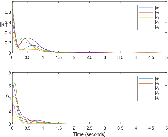
Figure 2: Trajectories of ‖ei‖\|e_{i}\| and ‖e˙i‖\|\dot{e}_{i}\|, for i=1,…,5i=1,\dots,5.
Refer to caption
Figure 3: Trajectories of ηi\eta_{i} and SiS_{i}, for i=1,⋯,5i=1,\cdots,5.

Consider a group of 5 EL agents with the communication network described in Figure 1. Let each EL agent represent a two-link robotic arm, whose dynamics is described by (1), with generalized coordinates qi=col​(θi​1,θi​2)q_{i}=\mbox{col}\left(\theta_{i1},\theta_{i2}\right),

ℳi​(qi)\displaystyle\mathcal{M}_{i}\left(q_{i}\right) =[ai​1+ai​2+2ai​3cosθi​2ai​2+ai​3cosθi​2ai​2+ai​3cosθi​2ai​2],\displaystyle=\left[\begin{array}[]{cc}a_{i1}+a_{i2}+2a_{i3}\cos\theta_{i2}&a_{i2}+a_{i3}\cos\theta_{i2}\\ a_{i2}+a_{i3}\cos\theta_{i2}&a_{i2}\\ \end{array}\right],
𝒞i​(qi,q˙i)\displaystyle\mathcal{C}_{i}\left(q_{i},\dot{q}_{i}\right) =[−ai​3​(sin⁡θi​2)​θ˙i​2−ai​3sinθi​2(θ˙i​1+θ˙i​2)ai​3sinθi​2θ˙i​10],\displaystyle=\left[\begin{array}[]{cc}-a_{i3}\left(\sin\theta_{i2}\right)\dot{\theta}_{i2}&-a_{i3}\sin\theta_{i2}\big(\dot{\theta}_{i1}+\dot{\theta}_{i2}\big)\\ a_{i3}\sin\theta_{i2}\dot{\theta}_{i1}&0\\ \end{array}\right],
Gi​(qi)\displaystyle G_{i}\left(q_{i}\right) =[ai​4gcosθi​1+ai​5gcos(θi​1+θi​2)ai​5​g​cos⁡(θi​1+θi​2)],\displaystyle=\left[\begin{array}[]{c}a_{i4}g\cos\theta_{i1}+a_{i5}g\cos\left(\theta_{i1}+\theta_{i2}\right)\\ a_{i5}g\cos\left(\theta_{i1}+\theta_{i2}\right)\\ \end{array}\right],

and Θi=col​(ai​1,ai​2,ai​3,ai​4,ai​5)\Theta_{i}=\mbox{col}\left(a_{i1},a_{i2},a_{i3},a_{i4},a_{i5}\right). This dynamics is adopted from Example 3.2-2 in [3] with some simplified modification of notations. The physical interpretation of each parameter can be found in [3]. We consider the disturbance

di​k=ψi​ksin(σi​kt+ϕi​k),k=1,2.d_{ik}=\psi_{ik}\sin\left(\sigma_{ik}t+\phi_{ik}\right),\penalty\ \penalty\ \penalty\ k=1,2.

According to the internal model approach, we can select

Φi​k=[01−σi​k20],Ψi​k=[10].\Phi_{ik}=\left[\begin{array}[]{cc}0&1\\ -\sigma_{ik}^{2}&0\\ \end{array}\right],\penalty\ \penalty\ \Psi_{ik}=\left[\begin{array}[]{cc}1&0\\ \end{array}\right].

Choosing

Mi​k=[01−3−2],Ni​k=[01],M_{ik}=\left[\begin{array}[]{cc}0&1\\ -3&-2\\ \end{array}\right],\penalty\ \penalty\ N_{ik}=\left[\begin{array}[]{c}0\\ 1\\ \end{array}\right],

gives

Ti​kσi​k=\displaystyle T_{ik}^{\sigma_{ik}}= [3−σi​k2−22​σi​k23−σi​k2]​1(3−σi​k2)2+4​σi​k2,\displaystyle\left[\begin{array}[]{cc}3-\sigma_{ik}^{2}&-2\\ 2\sigma_{ik}^{2}&3-{\sigma_{ik}^{2}}\\ \end{array}\right]\frac{1}{\left(3-\sigma_{ik}^{2}\right)^{2}+4\sigma_{ik}^{2}},
Ψi​k​(Ti​kσi​k)−1=\displaystyle\Psi_{ik}\left(T_{ik}^{\sigma_{ik}}\right)^{-1}= [3−σi​k22],\displaystyle\left[\begin{array}[]{cc}3-\sigma_{ik}^{2}&2\\ \end{array}\right],
Ti​k0=\displaystyle T_{ik}^{0}= [3−203]​19.\displaystyle\left[\begin{array}[]{cc}3&-2\\ 0&3\\ \end{array}\right]\frac{1}{9}.

Let σi=col​(σi​1,σi​2)\sigma_{i}=\mbox{col}\left(\sigma_{i1},\sigma_{i2}\right), ψi=col​(ψi​1,ψi​2)\psi_{i}=\mbox{col}\left(\psi_{i1},\psi_{i2}\right), ϕi=col​(ϕi​1,ϕi​2)\phi_{i}=\mbox{col}\left(\phi_{i1},\phi_{i2}\right), Mi=block diag​(Mi​1,Mi​2)M_{i}=\mbox{block diag}\left(M_{i1},M_{i2}\right), Ni=block diag​(Ni​1,Ni​2)N_{i}=\mbox{block diag}\left(N_{i1},N_{i2}\right), Ti=block diag​(Ti​1,Ti​2)T_{i}=\mbox{block diag}\left(T_{i1},T_{i2}\right), and Ψi=block diag​(Ψi​1,Ψi​2)\Psi_{i}=\mbox{block diag}\left(\Psi_{i1},\Psi_{i2}\right). For the nominal value σi=0\sigma_{i}=0, we have

Eiσi=\displaystyle E^{\sigma_{i}}_{i}= Ψi​(Ti0)−1−Ψi​(Tiσi)−1=[σi​1200000σi​220]\displaystyle\Psi_{i}\left(T_{i}^{0}\right)^{-1}-\Psi_{i}\left(T_{i}^{\sigma_{i}}\right)^{-1}=\left[\begin{array}[]{cccc}\sigma_{i1}^{2}&0&0&0\\ 0&0&\sigma_{i2}^{2}&0\\ \end{array}\right]
=\displaystyle= [1000000000001000]​[[ϱi​1ϱi​2]⊗I4]\displaystyle\left[\begin{array}[]{cccc|cccc}1&0&0&0&0&0&0&0\\ 0&0&0&0&1&0&0&0\\ \end{array}\right]\left[\left[\begin{array}[]{c}\varrho_{i1}\\ \varrho_{i2}\\ \end{array}\right]\otimes I_{4}\right]
=\displaystyle= [Ei​1Ei​2]​[ϱi⊗I4]\displaystyle\left[\begin{array}[]{cc}E_{i1}&E_{i2}\\ \end{array}\right]\left[\varrho_{i}\otimes I_{4}\right]
=\displaystyle= Ei​[ϱi⊗I4],\displaystyle E_{i}\left[\varrho_{i}\otimes I_{4}\right],

where ϱi=col​(ϱi​1,ϱi​2)=col​(σi​12,σi​22)\varrho_{i}=\mbox{col}\left(\varrho_{i1},\varrho_{i2}\right)=\mbox{col}\left(\sigma_{i1}^{2},\sigma_{i2}^{2}\right). Then, we have ωi=col​(Θi,ϱi⊗Θi,ϱi)\omega_{i}=\mbox{col}\left(\Theta_{i},\varrho_{i}\otimes\Theta_{i},\varrho_{i}\right). Next, the terms ρi​(qi,q˙i,si,ζi)\rho_{i}(q_{i},\dot{q}_{i},s_{i},\zeta_{i}) and Pi​(qi,q˙i,si)P_{i}(q_{i},\dot{q}_{i},s_{i}) can be obtained from the following equations

ρi​(qi,q˙i,si,ζi)=\displaystyle\rho_{i}(q_{i},\dot{q}_{i},s_{i},\zeta_{i})= [Ai​ζi+Qi​(qi,q˙i,si)Ei∘[ζi+N​Li​(qi,si)]Ei∘ξi],\displaystyle\left[\begin{array}[]{c}A_{i}\zeta_{i}+Q_{i}(q_{i},\dot{q}_{i},s_{i})\\ E_{i}\circ\left[\zeta_{i}+NL_{i}\left(q_{i},s_{i}\right)\right]\\ E_{i}\circ\xi_{i}\\ \end{array}\right],
Pi​(qi,q˙i,si)​Θi=\displaystyle P_{i}(q_{i},\dot{q}_{i},s_{i})\Theta_{i}= Mi​Ni​ℳi​(qi)​si+Ni​Ci​(qi,q˙i)​si\displaystyle M_{i}N_{i}\mathcal{M}_{i}\left(q_{i}\right)s_{i}+N_{i}C_{i}\left(q_{i},\dot{q}_{i}\right)s_{i}
−Ni​ℳ˙i​(qi)​si+Ni​Yi​(qi,q˙i,q˙r​i,q¨r​i)​Θi,\displaystyle-N_{i}\dot{\mathcal{M}}_{i}\left(q_{i}\right)s_{i}+N_{i}Y_{i}\left(q_{i},\dot{q}_{i},{\color[rgb]{0,0,0}\dot{q}_{ri},\ddot{q}_{ri}}\right)\Theta_{i},

with

Qi​(qi,q˙i,si)​Θi=\displaystyle Q_{i}(q_{i},\dot{q}_{i},s_{i})\Theta_{i}= Ai​Ni​ℳi​(qi)​si−Yi​(qi,q˙i,q˙r​i,q¨r​i)​Θi,\displaystyle A_{i}N_{i}\mathcal{M}_{i}\left(q_{i}\right)s_{i}-Y_{i}\left(q_{i},\dot{q}_{i},{\color[rgb]{0,0,0}\dot{q}_{ri},\ddot{q}_{ri}}\right)\Theta_{i},
Li​(qi,si)​Θi=\displaystyle L_{i}(q_{i},s_{i})\Theta_{i}= ℳi​(qi)​si.\displaystyle\mathcal{M}_{i}\left(q_{i}\right)s_{i}.

Now, we are ready to construct the control law as follows

τi\displaystyle\tau_{i} =−Ki​si−ρi​(qi,q˙i,si,ζi)​ω^i+Ai​ξi,\displaystyle=-K_{i}s_{i}-\rho_{i}(q_{i},\dot{q}_{i},s_{i},\zeta_{i})\hat{\omega}_{i}+A_{i}\xi_{i},
ξ˙i\displaystyle\dot{\xi}_{i} =Mi​ξi+Ni​τi,\displaystyle=M_{i}\xi_{i}+N_{i}\tau_{i},
ω^˙i\displaystyle\dot{\hat{\omega}}_{i} =Λ−1​ρiT​(qi,q˙i,si,ζi)​si,\displaystyle=\Lambda^{-1}\rho_{i}^{T}(q_{i},\dot{q}_{i},s_{i},\zeta_{i})s_{i},
ζ˙i\displaystyle\dot{\zeta}_{i} =Mi​ζi+Pi​(qi,q˙i,si),\displaystyle=M_{i}\zeta_{i}+P_{i}(q_{i},\dot{q}_{i},s_{i}),
S˙i\displaystyle\dot{S}_{i} =μ1​∑j=15ai​j​(Sj−Si),\displaystyle=\mu_{1}\sum\nolimits_{j=1}^{5}{a_{ij}(S_{j}-S_{i})},
η˙i\displaystyle\dot{\eta}_{i} =Si​ηi+μ2​∑j=15ai​j​(ηj−ηi).\displaystyle=S_{i}\eta_{i}+\mu_{2}\sum\nolimits_{j=1}^{5}{a_{ij}(\eta_{j}-\eta_{i})}.

Select the following parameters: μ1=μ2=2\mu_{1}=\mu_{2}=2, Ki=40​I2K_{i}=40I_{2}, α=6\alpha=6, Λi=0.15​I17\Lambda_{i}=0.15I_{17}. The actual values of Θi\Theta_{i}, ψi\psi_{i}, σi\sigma_{i} and ϕi​k\phi_{ik} are given as:

Θ1=\displaystyle\Theta_{1}= col​(0.64,1.10,0.08,0.64,0.32),ψ1=col​(6,8),\displaystyle\mbox{col}(0.64,1.10,0.08,0.64,0.32),\penalty\ \psi_{1}=\mbox{col}(6,8),
Θ2=\displaystyle\Theta_{2}= col​(0.76,1.17,0.14,0.93,0.44),ψ2=col​(−1,−2),\displaystyle\mbox{col}(0.76,1.17,0.14,0.93,0.44),\penalty\ \psi_{2}=\mbox{col}(-1,-2),
Θ3=\displaystyle\Theta_{3}= col​(0.91,1.26,0.22,1.27,0.58),ψ3=col​(−2,−5),\displaystyle\mbox{col}(0.91,1.26,0.22,1.27,0.58),\penalty\ \psi_{3}=\mbox{col}(-2,-5),
Θ4=\displaystyle\Theta_{4}= col​(1.10,1.36,0.32,1.67,0.73),ψ4=col​(3,5),\displaystyle\mbox{col}(1.10,1.36,0.32,1.67,0.73),\penalty\ \psi_{4}=\mbox{col}(3,5),
Θ5=\displaystyle\Theta_{5}= col​(1.21,1.16,0.12,1.45,1.03),ψ5=col​(−3,−2.5),\displaystyle\mbox{col}(1.21,1.16,0.12,1.45,1.03),\penalty\ \psi_{5}=\mbox{col}(-3,-2.5),

σi=col​(0.1,0.2)\sigma_{i}=\mbox{col}(0.1,0.2) and ϕi​k=0\phi_{ik}=0. The simulation is conducted with the following initial conditions: qi=0q_{i}=0, Θ^i=0\hat{\Theta}_{i}=0, ζi=0\zeta_{i}=0, ω^i=0\hat{\omega}_{i}=0, ξi=0\xi_{i}=0, ∀i\forall i, and

S1​(0)\displaystyle S_{1}\left(0\right) =[03−60],S2​(0)=[0−210],\displaystyle=\left[\begin{array}[]{cc}0&3\\ -6&0\\ \end{array}\right],\penalty\ \penalty\ S_{2}\left(0\right)=\left[\begin{array}[]{cc}0&-2\\ 1&0\\ \end{array}\right],
S3​(0)\displaystyle S_{3}\left(0\right) =[0−2−30],S4​(0)=[0−2−30],\displaystyle=\left[\begin{array}[]{cc}0&-2\\ -3&0\\ \end{array}\right],\penalty\ \penalty\ S_{4}\left(0\right)=\left[\begin{array}[]{cc}0&-2\\ -3&0\\ \end{array}\right],
S5​(0)\displaystyle S_{5}\left(0\right) =[02−30],η1​(0)=col​(0.2,0.5),\displaystyle=\left[\begin{array}[]{cc}0&2\\ -3&0\\ \end{array}\right],\penalty\ \eta_{1}\left(0\right)=\mbox{col}(0.2,0.5),
η2​(0)\displaystyle\eta_{2}\left(0\right) =col​(−0.6,0.3),η3​(0)=col​(−0.1,0.4),\displaystyle=\mbox{col}(-0.6,0.3),\penalty\ \eta_{3}\left(0\right)=\mbox{col}(-0.1,0.4),
η4​(0)\displaystyle\eta_{4}\left(0\right) =col​(−0.6,0.6),η5​(0)=col​(0.9,0.2).\displaystyle=\mbox{col}(-0.6,0.6),\penalty\ \eta_{5}\left(0\right)=\mbox{col}(0.9,0.2).

The errors in Figure 2 show that consensus of both qiq_{i} and q˙i\dot{q}_{i} is achieved among all the five agents. The trajectories of ηi\eta_{i} and SiS_{i} in Figure 3 show that all five agents converge to an autonomous system arising from the communication network, the inherent properties and the initial states of the agents.

VI Conclusion

This paper proposed a novel design for leaderless consensus and disturbance rejection problem of multiple Euler-Lagrange agents. In this setting, all agents must converge to a common behavior while being affected by persistent disturbances with unknown biases, amplitudes, initial phases and frequencies. The main feature of the proposed design is that none of the agents has information of a common reference model or of a common reference trajectory. Rather, all agents collaborate with each other through a communication network to achieve a common reference trajectory, and simultaneously reject persistent disturbances. The analysis shows that the generalized coordinates and velocities of the multiple Euler-Lagrange systems converge to common time-varying states in a distributed way.

References

  • [1] Z. Peng, J. Wang, and D. Wang, “Containment maneuvering of marine surface vehicles with multiple parameterized paths via spatial-temporal decoupling,” IEEE/ASME Transactions on Mechatronics, vol. 22, no. 2, pp. 1026–1036, 2016.
  • [2] Z. Chen and J. Huang, “Attitude tracking of rigid spacecraft subject to disturbances of unknown frequencies,” International Journal of Robust and Nonlinear Control, vol. 24, no. 16, pp. 2231–2242, 2014.
  • [3] F. L. Lewis, D. M. Dawson, and C. T. Abdallah, Robot Manipulator Control: Theory and Practice (Second Edition). New York: Marcel Dekker, 2004.
  • [4] G. Zarikian and A. Serrani, “External model-based disturbance rejection in tracking control of Euler-Lagrange systems,” in Proceedings of the American Control Conference, 2005, pp. 3562–3567.
  • [5] P. M. Patre, W. MacKunis, K. Dupree, and W. E. Dixon, “Modular adaptive control of uncertain Euler-Lagrange systems with additive disturbances,” IEEE Transactions on Automatic Control, vol. 65, no. 1, pp. 155–160, 2011.
  • [6] Z. Chen and J. Huang, “Attitude tracking and disturbance rejection of rigid spacecraft by adaptive control,” IEEE Transactions on Automatic Control, vol. 54, no. 3, pp. 600–605, 2009.
  • [7] M. Lu, L. Liu, and G. Feng, “Adaptive tracking control of uncertain Euler-Lagrange systems subject to external disturbances,” Automatica, vol. 104, pp. 207–219, 2019.
  • [8] E. Nuno, “Consensus of Euler-Lagrange systems using only position measurements,” IEEE Transactions on Control of Network Systems, vol. 5, no. 1, pp. 489–498, 2018.
  • [9] H. Cai and J. Huang, “The leader-following consensus for multiple uncertain Euler-Lagrange systems with an adaptive distributed observer,” IEEE Transactions on Automatic Control, vol. 61, no. 10, pp. 3152–3157, 2016.
  • [10] J. R. Klotz, T.-H. Cheng, and W. E. Dixon, “Robust containment control in a leader–follower network of uncertain Euler–Lagrange systems,” International Journal of Robust and Nonlinear Control, vol. 26, no. 17, pp. 3791–3805, 2016.
  • [11] W. Ren, “Distributed leaderless consensus algorithms for networked Euler-Lagrange systems,” International Journal of Control, vol. 82, no. 11, pp. 2137–2149, 2009.
  • [12] J. R. Klotz, Z. Kan, J. M. Shea, E. L. Pasiliao, and W. E. Dixon, “Asymptotic synchronization of a leader-follower network of uncertain Euler-Lagrange systems,” IEEE Transactions on Control of Network systems, vol. 2, no. 2, pp. 174–182, 2014.
  • [13] E. Nuno, I. Sarras, A. Loria, M. Maghenem, E. Cruz-Zavala, and E. Panteley, “Strict Lyapunov–Krasovskiĭ functionals for undirected networks of Euler-Lagrange systems with time-varying delays,” Systems & Control Letters, vol. 135, p. 104579, 2020.
  • [14] J. Mei, “Distributed consensus for multiple Lagrangian systems with parametric uncertainties and external disturbances under directed graphs,” IEEE Transactions on Control of Network Systems, vol. 7, no. 2, pp. 648 –659, 2019.
  • [15] T. Liu and J. Huang, “Leader-following consensus with disturbance rejection for uncertain Euler-Lagrange systems over switching networks,” International Journal of Robust and Nonlinear Control, vol. 29, no. 18, pp. 6638–6656, 2019.
  • [16] H. Cai and J. Huang, “Leader-following consensus of multiple uncertain Euler-Lagrange systems under switching network topology,” International Journal of General Systems, vol. 43, no. 3-4, pp. 294–304, 2014.
  • [17] S. Wang and J. Huang, “Adaptive leader-following consensus for multiple Euler-Lagrange systems with an uncertain leader system,” IEEE Transactions on Neural Networks and Learning Systems, vol. 30, no. 7, pp. 2188–2196, 2018.
  • [18] S. Rao and D. Ghose, “Sliding mode control-based autopilots for leaderless consensus of unmanned aerial vehicles,” IEEE Transactions on Control Systems Technology, vol. 22, no. 5, pp. 1964–1972, 2014.
  • [19] S. Baldi and P. Frasca, “Leaderless synchronization of heterogeneous oscillators by adaptively learning the group model,” IEEE Transactions on Automatic Control, vol. 65, no. 1, pp. 412–418, 2020.
  • [20] Y. Yan, Z. Chen, and R. H. Middleton, “Autonomous synchronization of heterogeneous multi-agent systems,” IEEE Transactions on Control of Network Systems, vol. 8, no. 2, pp. 940 – 950, 2021.
  • [21] Z. Hu, Z. Chen, and H. T. Zhang, “Necessary and sufficient conditions for asymptotic decoupling of stable modes in LTV systems,” IEEE Transactions on Automatic Control, vol. 66, no. 10, pp. 4546–4559, 2021.
  • [22] F. L. Lewis, H. Zhang, K. Hengster-Movric, and A. Das, Cooperative Control of Multi-Agent Systems: Optimal and Adaptive Design Approaches. London: Springer-Verlag, 2014.
  • [23] W. Ren and R. W. Beard, “Consensus seeking in multiagent systems under dynamically changing interaction topologies,” IEEE Transactions on Automatic Control, vol. 50, no. 5, pp. 655–661, 2005.
  • [24] H. Cai, F. L. Lewis, G. Hu, and J. Huang, “The adaptive distributed observer approach to the cooperative output regulation of linear multi-agent systems,” Automatica, vol. 75, pp. 299–305, 2017.
  • [25] A. Serrani, A. Isidori, and L. Marconi, “Semi-global nonlinear output regulation with adaptive internal model,” IEEE Transactions on Automatic Control, vol. 46, no. 8, pp. 1178–1194, 2001.
  • [26] A. Isidori, L. Marconi, and A. Serrani, Robust Autonomous Guidance: An Internal Model Approach. London: Springer-Verlag, 2003.
  • [27] A. Isidori, L. Marconi, and G. Casadei, “Robust output synchronization of a network of heterogeneous nonlinear agents via nonlinear regulation theory,” IEEE Transactions on Automatic Control, vol. 59, no. 10, pp. 2680–2691, 2014.
  • [28] V. Nikiforov, “Adaptive non-linear tracking with complete compensation of unknown disturbances,” European Journal of Control, vol. 4, no. 2, pp. 132–139, 1998.