Reinforcement Learning with
Dynamic Convex Risk Measures
Abstract
We develop an approach for solving time-consistent risk-sensitive stochastic optimization problems using model-free reinforcement learning (RL). Specifically, we assume agents assess the risk of a sequence of random variables using dynamic convex risk measures. We employ a time-consistent dynamic programming principle to determine the value of a particular policy, and develop policy gradient update rules that aid in obtaining optimal policies. We further develop an actor-critic style algorithm using neural networks to optimize over policies. Finally, we demonstrate the performance and flexibility of our approach by applying it to three optimization problems: statistical arbitrage trading strategies, financial hedging, and obstacle avoidance robot control.
Keywords Reinforcement Learning Dynamic Risk Measures Policy Gradient Actor-Critic Algorithm Time-Consistency Trading Strategies Financial Hedging Robot Control
1 Introduction
Reinforcement learning (RL) provides a (model-free) framework for learning-based control. RL problems aim at learning dynamics in the underlying data and finding optimal behaviors while collecting data via an interactive process. It differs from supervised learning that attempts to learn classification functions from labeled data, and unsupervised learning that seeks hidden patterns in unlabeled data. During the training phase, the agent makes a sequence of decisions while interacting with the data-generating process and observing feedback in the form of costs. The agent aims to discover the best possible actions by interacting with the environment and consistently updating their actions based on their experience, while often, also taking random actions to assist in exploring the state space – the classic exploration-exploitation trade-off (Sutton and Barto 2018).
In RL, uncertainty in the data-generating process can have substantial effects on performance. Indeed, the environmental randomness may result in algorithms optimized for “on-average” performance to have large variance across scenarios. For example, consider a portfolio selection problem: a risk-neutral optimal strategy (where one optimizes the expected terminal return) focuses on assets with the highest returns while ignoring the risks associated with them. As a second example, consider an autonomous car which should account for environmental uncertainties such as the weather and road conditions when learning the optimal strategy. Such an agent may wish to account for variability in the environment and the results of its actions to avoid large potential “losses”. For an overview and outlook on RL in financial mathematics see, e.g., Jaimungal 2022.
In the extant literature, there are numerous proposals for accounting for risk sensitivity, where most of them replace the expectation in the optimization problem by risk measures – we provide an overview in Section 2. Risk-awareness or risk-sensitivity in RL offers a remedy to the data-generating process uncertainty by quantifying low-probability but high-cost outcomes, provides strategies that are more robust to the environment, and allows more flexibility than traditional approaches as it is tuned to the agent’s risk preference. The specific choice of risk measure is a decision the agent makes considering their goals and risk tolerances. We do not address here how the agent makes this specific choice and instead refer the reader to, e.g., Dhaene et al. 2006 for an overview.
An interesting approach to risk-aware learning stems from Tamar et al. 2015; Tamar et al. 2016, where they provide policy search algorithms to solve risk-aware RL problems in a dynamic framework. Both studies investigate stationary policies, restrict themselves to coherent risk measures, and apply their methodology to simple financial engineering applications. More specifically, they evaluate their algorithms when learning policies for (perpetual) American options and trading in static portfolio optimization problems. Several real-world applications require a level of flexibility that these limitations preclude.
In this paper, we develop a model-free approach to solve a wide class of (non-stationary) risk-aware RL problems in a time-consistent manner. Our contributions may be summarized as follows: (i) we extend Tamar et al. 2015; Tamar et al. 2016; Ahmadi et al. 2020; Kose and Ruszczynski 2021; Huang et al. 2021 by focusing on the broad class of dynamic convex risk measures and consider finite-horizon problems with non-stationary policies; (ii) we devise an actor-critic algorithm to solve this class of RL problems using neural networks to allow continuous state-action spaces; (iii) we derive a recursive formula for efficiently computing the policy gradients; and (iv) we demonstrate the performance and flexibility of our proposed approach on three important applications: optimal trading for statistical arbitrage, hedging financial options, and obstacle avoidance in robot control. We demonstrate that our approach appropriately accounts for uncertainty and leads to strategies that mitigate risk.
The remainder of the paper is structured as follows. In Section 2, we discuss related work and introduce our RL notation in Section 3. Section 4 formalizes the evaluation of risk in both static and dynamic frameworks. We introduce the class of sequential decision making problems with dynamic convex risk measures in Section 5 and devise an actor-critic style algorithm to solve them in Section 6. Finally, Section 7 illustrates the performance of our proposed algorithm, and we discuss our work’s limitations and possible extensions in Section 8.
2 Related Work
The literature in risk evaluation for sequential decision making can be divided between those that apply a risk measure to a single cost random variable (e.g. discounted sum of costs or terminal profit and loss), and those that apply risk measures recursively to a sequence of cost random variables (e.g. cash-flows). The former approach optimizes the risk of a single random variable, which does not account for the temporal structure in what generates it, while the latter optimizes the risk of sequences of random variables in a dynamic framework as additional information becomes available.
Several authors address sequential decision making problems by minimizing the risk of a cost over a whole episode. For example, Prashanth and Ghavamzadeh 2013 focus on objective functions for variance related criteria, while Chow et al. 2017 take a risk-constrained approach with an objective function that includes a penalty on the conditional value-at-risk (CVaR). Some lines of research look at risk-sensitive RL problems using a broader classes of risk measures, such as comonotonic (Petrik and Subramanian 2012), entropic (Nass et al. 2019), or spectral (Bäuerle and Glauner 2020b) risk measures. Di Castro et al. 2019 consider a risk-neutral objective function, but includes an additional constraint on the risk of the cumulative discounted cost.
Other works extend optimization in Markov decision processes (MDPs) by evaluating the risk at each period. For instance, Ruszczyński 2010 evaluates the risk at each period using dynamic Markov coherent risk measures, while Chu and Zhang 2014 and Bäuerle and Glauner 2021 propose iterated coherent risk measures, where they both derive risk-aware dynamic programming (DP) equations and provide policy iteration algorithms. While they focus on coherent risk measures, various classes of risk measures have already been extended to a dynamic framework, such as distribution-invariant risk measures (Weber 2006), coherent risk measures (Riedel 2004), convex risk measures (Frittelli and Gianin 2004; Detlefsen and Scandolo 2005), and dynamic assessment indices (Bielecki et al. 2016), among others – however, these works do not look at how to perform model free optimization, i.e., they do not look at RL. For an overview of dynamic risk measures, see, e.g., Acciaio and Penner 2011.
Another way to account for uncertainty in the data-generating process is by allowing the parameters of the model, or the entire distribution itself, to be unknown. The class of robust MDPs (Delage and Mannor 2010) focuses on optimizing the worst-case expectation when the parameters vary within a certain set. There exists relationships between risk-aware and robust MDPs, as shown in Osogami 2012 and Bäuerle and Glauner 2020a. Indeed, minimizing a Markov coherent risk measure in a risk-aware context is equivalent to minimizing a certain worst-case expectation where the uncertainty set is characterized by a concave function. Several researchers have developed algorithms to solve robust MDPs, for an overview see, e.g., Rahimian and Mehrotra 2019.
While we consider a model-free approach, several researchers tackle related, but distinct, problems in a model-based framework. For instance, Weinan et al. 2017 and Han et al. 2018 use deep learning methods to solve non-linear partial differential equations (PDEs). Using the non-linear Feynman-Kac representation, they reformulate the PDEs as backward stochastic differential equations (BSDEs), they then parametrize the co-adjoint process and initial condition using an ensemble of neural networks, and use the mean squared error in the terminal condition as the loss function. Despite there being an equivalence between BSDEs and dynamic risk measures (Peng 1997; Drapeau et al. 2016), the dual representation does not directly help when we aim to optimize a dynamic risk measure in a model-free manner.
Other types of algorithms exist in the literature to find a solution to risk-aware RL problems. Among others, Galichet et al. 2013 use a multi-armed bandit approach, Shen et al. 2014 devise a risk-sensitive Q-learning method when optimizing utility functions, Bellemare et al. 2017 use a distributional perspective to learn the whole distribution of the value function, Yu et al. 2018 employ an approximate DP approach to devise a value iteration algorithm for Markov risk measures, and Kalogerias et al. 2020 address risk-aware problems from a Bayesian perspective. The shortcomings of these approaches are that they apply to a specific class of risk measures and the developed methodologies are tuned to them.
3 Reinforcement Learning
In this section, we introduce the necessary theoretical background for the RL problems we study. We describe each problem as an agent who tries to learn an optimal behavior, or agent’s policy, by interacting with a certain data-generating process.
Let and be arbitrary state and action spaces respectively, and let be a cost space. The data-generating process is often represented as a MDP with the tuple , where is a deterministic, state-action dependent cost function and characterizes the transition probabilities , unknown to the agent. The transition probability is assumed stationary, although time may be a component of the state, e.g. we usually assume that time is embedded in the state space without loss of generality. A single episode consists of periods, where is known and finite. At each period, the agent begins in state , takes an action , moves to the next state , and receives a cost . A directed graph representation of the described MDP is shown in Fig. 1. A trajectory consists of all states, actions and costs that occur during a single episode and we denote it by the tuple .
The agent follows a strategy described by a randomized (also known as exploratory control) policy , where is the space of probability measures on . More specifically when in state at time , the agent selects the action with probability . This also allows for non-stationary policies when dealing with finite-horizon problems.
Standard RL usually deals with risk-neutral objective functions of the (-discounted) cost of a trajectory induced by a MDP with a policy , for instance
| (1) |
where is a discount factor. At period , there is no action and hence any cost based on the terminal state is encapsulated in . Contrastingly, risk-sensitive RL considers problems in which the objective takes into account the variability of the cost with a risk measure , whether optimizing
| (2) |
or Eq. 1 with an additional constraint on the risk measure of the trajectory cost. We discuss thoroughly risk measures and their properties in Section 4 next.
In all cases, the goal of RL is to learn the optimal policy that attains the minimum in the corresponding objective function, and do so in a manner that makes no explicit assumptions on the data-generating process.
4 Risk Measures
In this section, we formalize how we quantify the risk of random variables. We start by providing a review of static risk measures, and then continue by reviewing the framework of Ruszczyński 2010 for building time-consistent dynamic risk measures. Static risk measures evaluate the immediate risk of a financial position, while dynamic risk measures allow its monitoring at different times, and lead to time-consistent optimal strategies. In our work, we make use of static risk measures on conditional distributions of random variables to construct dynamic risk measures.
4.1 Static Setting
Let be a probability space, the extended real line, and define and with such that . They represent the space of -integrable, respectively -integrable, -measurable random variables. A risk measure is a mapping , where is a space of random variables, that satisfies additional properties. In what follows we assume that and is interpreted as a random cost. We next enumerate some properties of various risk measures.
Definition 1.
Let , and . A map is said to be
- 1.
law-invariant if if ;
- 2.
monotone if implies ;
- 3.
translation invariant if ;
- 4.
positive homogeneous if ;
- 5.
comonotonic additive if for all comonotonic pairs ;
- 6.
subadditive if ;
- 7.
convex if .
There is a consensus in the literature that any risk measure should satisfy the monotonicity and translation invariance properties. More specifically, a portfolio with a higher cost for every possible scenario is indeed riskier, and the deterministic part of a portfolio does not contribute to its risk.
Definition 2.
A map is said to be a monetary risk measure (Föllmer et al. 2004) if and only if it is monotone and translation invariant.
In addition to being monetary, additional requirements may be assumed so that the risk measure reflects observed investor behavior.
Definition 3.
A map is said to be a coherent risk measure (Artzner et al. 1999) if and only if it is monotone, translation invariant, positive homogeneous, and subadditive.
The additional properties for coherent risk measures guarantees that doubling a position doubles its risk, and diversifying a portfolio reduces its risk. The CVaR (Rockafellar et al. 2000) is a well-known example of a coherent risk measure commonly used in the literature. Criticisms of positive homogeneity and subadditivity led to the study of a broader class of risk measures, where these axioms are weakened and replaced by the notion of convexity. Indeed, the risk might increase in a nonlinear way, which is not permitted under coherent risk measures.
Definition 4.
A map is said to be a convex risk measure (Föllmer and Schied 2002) if and only if it is monotone, translation invariant, and convex.
Another advantage of convex risk measures is that we can combine several risk measures into a linear combination to create a trade-off between different risk-aware objectives. Indeed, one can easily show that given two convex risk measures and nonnegative coefficients , then and are both also convex. The set of coherent risk measures is a strict subset of the set of convex risk measures.
A dual representation of convex (and, as a special case, coherent) risk measures provides us with a key result for developing our practical algorithm. The dual representation requires us to introduce the expectation under what is effectively a distorted probability measure and denote with and .
Definition 5.
The conjugate (Shapiro et al. 2014) of the risk measure , denoted , is given by
| (3) |
Definition 6.
The biconjugate (Shapiro et al. 2014), or conjugate of the conjugate, is a mapping with
| (4) |
The dual representation of the risk measure is given in the following theorem.
Theorem 7 (Representation Theorem (Shapiro et al. 2014, see Theorem 6.4 in)).
A convex risk measure is proper (i.e. and its domain is nonempty) and lower semicontinuous (i.e. ) iff there exists a set
often referred to as the risk envelope, such that
| (5) |
Moreover, we have that is coherent (e.g. satisfies also the positive homogeneity) iff
If we assume is a convex, proper, lower semicontinuous risk measure, then by Theorem 7, it may be written as an optimization problem where the distortion is chosen adversarially from a subset of the set of all probability densities. Moreover, the notable difference between coherent and convex risk measures is the conjugate term that appears in its dual representation. Coherent risk measures are uniquely characterized by their risk envelope.
4.2 Dynamic Setting
Optimizing a controlled performance criteria using static risk measures is known to lead to time-inconsistent solutions – we discuss the precise definition below. Adapting risk measures to properly account for the flow of information requires additional care to ensure that the risk evaluation is done in a time-consistent manner, especially with DP models for MDPs. There are multiple extensions of static risk measure to the dynamic case. Indeed, various classes of risk measures have already been extended to a dynamic framework, such as distribution-invariant (Weber 2006), coherent (Riedel 2004), convex risk measures (Frittelli and Gianin 2004; Detlefsen and Scandolo 2005), and dynamic assessment indices Bielecki et al. 2016, among others. Here we closely follow the work of Ruszczyński 2010.
To this end, let denote the sequence of periods in an episode. Consider a filtration on a filtered probability space and with . Define .
Definition 8.
A conditional risk measure is a map which satisfies the monotonicity property, i.e. for all such that a.s..
Definition 9.
A dynamic risk measure is a sequence of conditional risk measures .
We may interpret , for , as a -measurable charge the agent would be willing to incur at time instead of the sequence of costs . Developing a dynamic programming principle (DPP) for dynamic risk measures crucially depends on the property of time-consistency. One wishes to evaluate the risk of future outcomes, but it must not lead to inconsistencies at different points in time.
Definition 10.
is said to be time-consistent (Ruszczyński 2010, see Definition 3 in) iff for any sequence and any such that (),
implies that .
Definition 10 may be interpreted as follows: if will be at least as good as at time and they are identical between and , then should not be worse than at time .
Furthermore, we introduce one additional concept that aids in developing a recursive relationship for dynamic risk measures.
Definition 11.
A one-step conditional risk measure is a map which satisfies for any .
One may assume even stronger properties for conditional risk measures, e.g., one may assume the risk measures are static (across time) and convex. In the next section, we do precisely this. Therefore, the one-step conditional risk measure outputs an -measurable random variable obtained when conditioning on . As a consequence of Definitions 10 and 11, we have the following recursive relationship for time-consistent dynamic risk measures.
Theorem 12 (Recursive relationship (Ruszczyński 2010, see Theorem 1 and Eq. (10) in)).
Let be a time-consistent, dynamic risk measure. Suppose that it satisfies and for any , . Then can be expressed as
| (6) |
As we are working with MDPs, the agent observes at each period the current state , that is -measurable. We thus define dynamic Markov risk measures, in a similar manner to Ruszczyński 2010, where are Markov one-step conditional risk measures that are -measurable. Those are originally obtained from risk transition mappings with respect to a controlled Markov process, which our framework with MDPs satisfies (for a thorough exploration, see Ruszczyński 2010, especially Section 4).
5 Problem Setup
In this section, we formally introduce the optimization problems that we face. Briefly, we are interested in RL problems where the agent wants to minimize a dynamic convex risk measure in order to obtain a time-consistent solution.
Let be a MDP, be the sequence of periods in an episode, and suppose that the agent’s policy is parametrized by some parameters . We consider a time-consistent, Markov, dynamic convex risk measure , i.e. the one-step conditional risk measures are static convex risk measures, real-valued and lower semicontinuous. Using Eq. 6 from Theorem 12, we aim to solve the following -period risk-sensitive RL problem:
| (P1) |
where is a -measurable random cost and the trajectory may be modulated by the policy – that is why we include a index to actions and states. In the sequel, we may omit the superscript when obvious for readability purposes.
Let us denote transition probabilities by and -weighted conditional expectations by for any .
All one-step conditional risk measures of the dynamic risk measure satisfy the assumptions in Theorem 7, and thus using the dual representation from Theorem 7, the problem in Eq. P1 may be written equivalently as
| (P2) |
Assumption 13.
We restrict to convex risk measures such that the risk envelope may be written as
| (7) |
where are affine functions wrt , are convex functions wrt , and (resp. ) denotes the finite set of equality (resp. inequality) constraints. Furthermore, for any given , and are twice differentiable in , and there exists such that for all we have
As noted by Tamar et al. 2016, “all coherent risk measures we are aware of in the literature are already captured by [that] risk envelope”. Note, however, here we use convex (which subsumes coherent) risk measures, while still keeping the structure of the risk envelope induced by this observation for coherent risk measures. This risk envelope still covers most cases of convex risk measures typically of interest in the literature such as entropic risk measures, with Shannon entropy as the convex penalty , and more generally expected utility risk measures (Rockafellar and Uryasev 2013, see e.g.). Hence, we view the restrictions of 13 on the explicit form of as being not too restrictive.
We now wish to derive DP equations with a view of solving problems of the form (P2). To this end, define the value function as the running risk-to-go
| (8) |
for all and . Here, as is standard in the RL literature, the value function is to be understood as a tool to evaluate the quality of a given policy at any state of the MDP. In our case, it represents the risk at a certain time when being in a specific state and following the policy . The DP equations (DPE) for a specific policy are
| (9a) | ||||
| (9b) | ||||
for any and . The DPE allows us to recursively assess the full extant of the risk associated with a fixed policy , and in particular the recursion can be seen to include the risk associated with the current (random) cost and the one-step ahead running risk-to-go, both of which depend explicitly on the next state. Using the dual representation in Theorem 7, the DPE in Eqs. 9a and 9b may be written as
| (10a) | ||||
| (10b) | ||||
where denotes the conditional expectation .
We aim to optimize the value function over policies using a policy gradient approach (Sutton et al. 2000). Policy gradient proposes to optimize by updating parameters of the policy using the update rule , which requires an estimation of the gradient. In order to obtain the gradient of , we need an additional assumption on the transition probabilities, more specifically on the policy.
Assumption 14.
We suppose the logarithm of transition probabilities is a differentiable function in when , and its gradient wrt is bounded for any .
14 is written for completeness, as it is a common restriction with policy gradient methods (Sutton et al. 2000, see e.g.). It ensures that the agent chooses a differentiable policy so that policy gradient can be applied. Indeed, the transition probabilities depend on the policy’s parameters only through the policy itself – therefore, the gradient of the log-probability of a transition may be represented as
| (11) |
Theorem 15 provides the gradient formulae in our proposed methodology.
Theorem 15 (Gradient of ).
Proof of Theorem 15.
In order to have an expression for the gradient of the value function, we first compute the gradient of the last period and then obtain the recursive relation for subsequent periods. Using Theorem 7 and 13, the Lagrangian of the maximization problem in Eq. 10a (with ) for any state can be written as
| (13) |
By the convexity of Eq. 10a and 13, in Eq. 13 has at least one saddle-point. We emphasize here that the saddle-points depend on the state . Using Slater’s condition and the convexity of the problem, strong duality holds, i.e.
| (14) |
We then recall a what is known in the ML literature as the “likelihood-ratio” trick, which states that
| (15) |
Next, we apply the Envelope theorem for saddle-point problems (Milgrom and Segal 2002, see Theorem 4 and Corollary 5 in) – which relies on the equidifferentiability of the objective function and the absolute continuity of its gradient. These properties are satisfied as we work under 13. Under these assumptions, we have
which implies that the gradient wrt of the objective function equals to the gradient wrt of the Lagrangian evaluated at one of its saddle-points.
Using 14, the Envelope theorem, the Lagrangian in Eq. 13, the strong duality in Eq. 14 and the “likelihood-ratio” trick in Eq. 15, we obtain that
| (16) | ||||
The gradient for others periods is obtained in a similar manner. The Lagrangian of the problem in Eq. 10b (with ) is
| (17) |
As the value function depends on the policy , the gradient formula will have an additional term. We obtain
| (18) | ||||
This concludes the proof. ∎
While the term appears at first not to depend on the policy, and therefore the term in Theorem 15 appears to vanish, this is not necessarily so. To see why, let us consider convex penalties of the form for convex functions . In this case, using the Envelope theorem (Milgrom and Segal 2002) and the “likelihood-ratio” trick – the derivation is similar to the proof of Theorem 15 – the gradient wrt the policy is given by
While we do not restrict to the above specific form for , this result illustrates why, in general, this contribution to the gradient cannot be ignored.
6 Actor-Critic Algorithm
In this section, we provide details on our proposed algorithm and the architecture of the implemented objects. Our policy gradient algorithm has an actor-critic style (Konda and Tsitsiklis 2000), in the sense that we must learn two functions, and we do so in an alternating fashion: (i) a value function , which plays the role of the critic; and (ii) the policy , which plays the role of the actor. Actor-critic algorithms are on-policy policy search methods that maintain an estimate of a value function, which is then used to update the agent’s policy parameters. Such algorithms have been developed in the RL community for their ability to find optimal policies using low variance gradient estimates (Grondman et al. 2012). To obtain an approximation of the optimal policy, we perform the steps described in Algorithm 1.
We propose to use function approximations, more specifically neural network structures, as they are useful when dealing with continuous state-action spaces and are known to be universal approximators. In recent years, deep neural network modeling has shown remarkable success in approximating complex functions (LeCun et al. 2015; Silver et al. 2016; Goodfellow et al. 2016, see e.g.), especially in financial mathematics (Al-Aradi et al. 2018; Hu 2019; Casgrain et al. 2019; Cuchiero et al. 2020; Horvath et al. 2021; Campbell et al. 2021; Carmona and Laurière 2021; Ning et al. 2021; Hambly et al. 2021, see e.g.). The use of compositions of simple functions (usually referred to as propagation and activation functions) through several layers approximates complicated functions to arbitrary accuracy (with arbitrarily large structures). Neural networks also avoid the curse of dimensionality issue of representing nonlinear functions in high dimensions.
There are several approaches for modeling the policy and value function with neural network structures. We consider a policy characterized by a single (fully-connected, multi-layered feed forward) artificial neural network (ANN) with parameters , which takes a state and time as inputs and outputs a distribution over the space of actions . We also suppose that the value function is characterized by another single (fully-connected, multi-layered feed forward) ANN with parameters . approximates the value function when the system is in state during the period under policy , previously denoted in Eqs. 10a and 10b. We therefore refer to the policy and value function respectively by and .
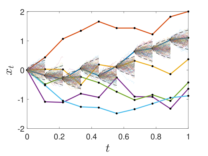
Our proposed algorithm uses a nested simulation or simulation upon simulation approach, where we simulate transitions at each visited state. This simulation upon simulation approach results in full (outer) episodes and batches of (inner) transitions for every state, as illustrated in Fig. 2. This allows us to easily compute and estimate quantities of interest for each state, e.g. saddle-points or one-step conditional risk measures. Such nested simulation approaches are computationally expensive – part of our future work aims to develop a more efficient algorithm when simulations are costly.
We next provide additional details on our actor-critic algorithm in Algorithm 1, i.e. how to (i) estimate the value function in Section 6.1 (step 5), and (ii) update the policy in Section 6.2 (step 7). Additional implementation details are provided in Appendix A.
6.1 Value Function Estimation
The value function may be estimated by using the recursion in Eqs. 10a and 10b. We use the simulation upon simulation approach mentioned previously. More precisely, when sampling a certain state , we also generate (inner) transitions from the policy to obtain the tuples , . We can then estimate the one-step conditional risk measures for any given state using those additional transitions. To update the value function, we perform this simulation process for a mini-batch of states, compute the predicted (i.e. output of ) and target values (i.e. Eqs. 10a and 10b), and calculate the expected square loss between these values. We update the parameters using the Adam optimizer (Kingma and Ba 2014) and repeat this process for several epochs in order to provide a good approximation of the value function. We recall that the policy is fixed while we optimize . The algorithm is provided in Algorithm 2.
else 8
Compute the expected square loss between and ; 9
A powerful result for neural networks structures is the universal approximation theorem – see e.g. Cybenko 1989; Hornik 1991; Leshno et al. 1993; Pinkus 1999.
Theorem 16 (Universal Approximation (Cybenko 1989)).
Let and be an activation function. Then is not a polynomial iff for any continuous function , any compact subset and any , there exists a neural network with representation such that .
We prove next that for a fixed policy , we can approximate its corresponding value function with an ANN using the procedure devised in Algorithm 2. Theorem 17 follows from the universal approximation theorem.
Theorem 17 (Approximation of ).
Let denote a fixed policy, with corresponding value function as defined in Eq. 8, which we denote . Then for any , there exists an ANN such that , for any .
Proof of Theorem 17.
First, we prove a lemma that states convex risk measures are absolutely continuous since they are in fact monetary. In what follows, the norm is to be understood as the -norm.
Lemma 18.
Monetary one-step conditional risk measures are absolutely continuous a.s..
Proof of Lemma 18.
Indeed, starting from the inequality , where , and using the monotonicity and translation invariance properties, we have
| (19) |
Repeating this with yields to
| (20) |
Therefore convex risk measures are Lipschitz continuous a.s. wrt the essential supremum norm, and hence they are absolutely continuous a.s.. ∎
Next, recall that the value function given in Eq. 8 is a dynamic convex risk measure, and therefore may be written recursively with the DPE in Eqs. 9a and 9b as
| (21) |
We prove that the ANN approximate the value function by induction. Without loss of generality, let us consider the case where the first dimension of the state space corresponds to the time . At the period , we have that
| (22) |
This is a convex risk measure which is absolutely continuous a.s. by Lemma 18. Using the universal approximation theorem given in Theorem 16, we obtain that for any , there exists a neural net such that
| (23) |
This proves the base case of our proof by induction.
For the induction step, the ANN approximates the value function at period as long as the value function at the next period is adequately approximated. Assume that for any , there exists an ANN such that
| (24) |
Using the translation invariance, the triangle inequality, Lemma 18 and Eq. 24, we have
| (25) |
Using the universal approximation theorem on Eq. 25, we get for any , there exists an ANN such that
| (26) |
We apply this argument recursively for any period , which completes the proof by induction.
Finally, we need an additional lemma to prove one can approximate the ensemble of ANNs with a single ANN .
Lemma 19.
Suppose , is an ensemble of a finite number of ANNs. Then for any , there exists an ANN such that , .
Proof of Lemma 19.
Throughout the proof, we label the ensemble using without loss of generality. We create an extension of the ensemble to obtain a function that is absolutely continuous a.s. wrt both and .
First, note that, by construction, ’s are absolutely continuous a.s. wrt . Between each pair of indices and , we extend the function via a polynomial interpolation on the compact set . Since we work on a closed interval and polynomials are continuously differentiable, the interpolation must be Lipschitz, and thus absolutely continuous. We then use this argument on all pairs of indices, which shows that there exists a function such that (i) for any and , and (ii) is absolutely continuous on .
Using the universal approximation theorem, for any , there exists an ANN such that
| (27) |
This also holds for , which yields the desired result. ∎
Using the triangle inequality and Lemma 19, for any , there exists an ANN such that
| (28) |
As Theorem 16 is valid for any , we can perform the training procedure in order to construct a sequence of that satisfies a global error , such as . ∎
6.2 Update of the Policy
The update of the policy is done using the gradients provided in Eqs. 12a and 12b of Theorem 15. Some points worth mentioning concern the policy, the saddle-points, and the gradient formula. When implementing the algorithm, we ensure the policy uses the so-called reparametrization trick, which allows the existence of pathwise gradient estimators from random samples. Usually there are three basic approaches to perform a reparametrization:
- (i)
Use a location-scale transformation – we can view the standard random variable as an auxiliary variable (such as ) and simulate (distributed as );
- (ii)
Use the inverse cumulative distribution function – if it is tractable, we can use the inverse transform sampling method to simulate realizations from uniform random variables;
- (iii)
Use a transformation of auxiliary variables – common examples are the log-normal distribution, which can be expressed by exponentiation of a Gaussian distribution, and the gamma distribution, which can be rewritten as a sum of exponentially distributed random variables.
Also since we assume the form of the risk envelope is known in an explicit form in 13, we can obtain a saddle-point of the Lagrangian of Eqs. 10a and 10b for any given risk measure, either analytically or using a sample average approximation (Shapiro et al. 2014, see Chapter 5 of). The approach to obtain these saddle-points is illustrated for common risk measures in Section 7.
We recall that the value function is fixed while we optimize . When we compute the gradient of the value function to optimize the policy, we fix the parameters of the value function . This can be interpreted as taking a copy of the ANN structure, which implies that the value function used in the actor part of the algorithm does not depend explicitly on . Therefore, the additional expectation of the gradient of the value function at in Eq. 12b vanishes. The value function gradient is then estimated averaging over a batch of states and different periods. The algorithm is given in Algorithm 3.
7 Experiments
In this section, we provide three illustrative examples to understand the potential gain of using dynamic risk measures in RL, and more specifically the advantages of our proposed approach on several examples. In our experiments, we consider several risk measures in order to compare their performance and highlight their differences.11 1 We implemented more dynamic convex risk measures in our code available on Github, and users can easily add their own in the Python files – see Appendix A for a description of the code architecture.
The first risk measure we consider is the dynamic expectation, where the one-step conditional risk measures are , which serves as a benchmark for the risk-neutral approach. It is a convex risk measure, and its saddle-point is given by and .
The second risk measure is the dynamic conditional value-at-risk (CVaR) with threshold , where the one-step conditional risk maps are
| (29) |
where
| (30) |
The CVaR is a coherent risk measure widely used in the financial mathematics literature (Rockafellar et al. 2000). As shown in Shapiro et al. 2014, any saddle-point satisfies if and otherwise, where is any -quantile of . Here, note that despite the static CVaR not being time-inconsistent (see Cheridito and Stadje 2009), the dynamic CVaR is time-consistent by construction.
The third risk measure is a dynamic penalized CVaR where we add a relative entropy term with respect to the uniform distribution. This is a convex but not coherent dynamic risk measure. The one-step conditional risk measures are given by
| (31) |
with the same risk envelope given in Eq. 30. Obtaining saddle-points is not as straightforward as with the CVaR, since it requires solving a convex optimization problem. The Lagrangian with the risk envelope constraints is
| (32) |
with and for all . Setting the derivative of Eq. 32 wrt to zero leads to
| (33) |
When imposing the constraint on the ’s on Eq. 33, we obtain the following expression
| (34) |
and that constraint is active when . We combine Eq. 34 with the constraint on to get
| (35) |
Any saddle-point then satisfies , where is a root of Eq. 35.
We note here that the penalized CVaR contains both risk measures as special cases. Indeed, for , it reduces to the CVaR, while we recover the expectation as tends to .
7.1 Statistical Arbitrage Example
This collection of experiments is performed on an algorithmic trading environment problem. The agent begins each episode with zero inventory, and on each period the agent wishes to trade quantities of an asset, whose price fluctuates according to some data-generating processes. For each period , the agent observes the asset’s price and their inventory , performs a trade , resulting in wealth according to
| (36) |
with coefficients and for the cost transactions and terminal penalty imposed by the market respectively. We suppose that , , , and the asset price follows an Ornstein-Uhlenbeck process, and hence mean-reverts:
| (37) |
where , , and is a standard -Brownian motion.22 2 Our approach is model-free, which implies that we can easily replace the asset price dynamics with more complex models, for instance including a stochastic volatility. The risk-aware agent tries to optimize the RL problem stated in Eq. P1, where for all periods , the actions are determined by the trades , the costs by the differences in wealth , and the states by the tuples .


Figure 3 shows a comparison of the learned policy between the dynamic expectation, the dynamic CVaR with and the dynamic penalized CVaR with and . When optimizing a risk-neutral objective function (see Figs. 3(a), 3(b), 3(c), and 3(d)), in the beginning of the episode, the agent aims to sell quantities of the asset when its price is higher than the mean-reversion level, and buy it when its price is lower. As periods evolve, the pattern shifts to ensure that the agent concludes the episode with zero inventory to avoid the terminal penalty. With other dynamic risk measures (see Figs. 3(e), 3(f), 3(g), 3(h), 3(i), 3(j), 3(k), and 3(l)), we observe that the agent is less aggressive, and instead waits until there are more significant price deviations from the mean-reversion level before taking actions that would benefit from the price reverting back to its mean. This reflects the risk-sensitive behavior of the agent.
The distribution of the terminal reward when the agent follows the learned policy for the dynamic mean, CVaR, and penalized CVaR is illustrated in Fig. 4. In general, risk-sensitive approaches lead to a distribution with a smaller variance and fewer large losses. The agent’s tolerance to risk can be adjusted by modifying the threshold of the dynamic CVaR (see Fig. 4(a)) or the relative entropy penalty constant of the dynamic penalized CVaR (see Fig. 4(b)). When increasing or , the distribution of the terminal wealth converges to the distribution for the risk-neutral objective function, as expected.
7.2 Hedging with Friction Example
A corner stone problem of mathematical finance is the question of how to hedge the exposure to financial options. In this section, we illustrate how our approach may be applied to hedging a call option in an environment where the underlying asset dynamics follows the Heston 1993 model in a market with trading frictions. In principle, one can swap out the specific stochastic volatility model for other models and/or use historical sample paths.
We denote the price of an underlying asset by and the call option’s strike price by . We consider the case where an agent sells the call option and aims to dynamically hedge it trading solely in the underlying asset and the bank account. We assume there are periods (corresponding to one month). Hence, the agent must pay at the terminal time.
We denote the stochastic variance process by , and, as a reminder, in the Heston model the price evolution of the underlying asset is given by
| (38a) | ||||
| (38b) | ||||
where is the drift, the mean-reversion rate, the mean-reversion level, the volatility of the volatility (often referred to as vol-vol), and are two -Brownian motions with correlation (i.e. ).
For generating sample paths, we use the Milstein discretization scheme (Mil’shtejn 1975) to simulate the dynamics of the stock price and volatility, where for each ,
| (39a) | ||||
| (39b) | ||||
with , , and the initial price and volatility respectively of and .
At each period , the agent’s wealth is determined by its hedges and bank account . In what follows, we assume: (i) there are market frictions in the form of transaction costs of (per share); (ii) the interest rate of the bank account, denoted , is zero; and (iii) the agent starts with an initial wealth of .
We next describe the dynamic hedging procedure we employ and the cash-flow it induces. For each , the agent takes an action , which corresponds to the number of shares to hold over the next time interval, based on its policy, and this action influences its bank account and wealth in the following manner:
| (40a) | ||||
| (40b) | ||||
The second term in represents the rebalancing costs, while the third term represents a cost due to trading frictions. The asset price, and bank account, evolves over the next period and induces a change in the agent’s wealth process. Thus, for each , we have the following relationships:
| (41a) | ||||
| (41b) | ||||
At the end of the investment horizon, the agent must pay the call option and liquidate its inventory. Therefore, we have
| (42a) | ||||
| (42b) | ||||
In our RL notation, the agent minimizes a dynamic convex risk measure of the costs induced by its policy, where for all periods , the costs are given by the change in the agent ’s wealth process , and the states represent all the information the agent possesses before making its hedging decision. Depending on the option and the market assumptions, one may easily include several features into the state space, such as more asset price history, market volatility, inventories of other assets the agent holds, and so on. To keep the experiments brief, here, we focus on just a few features.
We consider the case where the states that determine the agent’s policy are tuples of the form . Typically, in continuous time financial modeling for the Heston model, one assumes that the volatility process is observed and used as a feature in obtaining the optimal hedge. Here, however, we exclude it from the policy as in real-world trading, volatility itself is not observable. The initial wealth is obtained by forcing the dynamic risk (whether the dynamic CVaR at level or dynamic penalized CVaR at level with relative entropy penalty constant ) to be . This specific choice is up to the agent to choose and represents the minimal reservation value the agent is willing to take. In implementation, we achieve this by initially setting the price to the Black-Scholes price using the long-run volatility , and then adjusting the price until the dynamic risk is . As coherent and convex dynamic risk measures are translation invariant (see Definitions 3 and 4), the learned policy is not affected by this price adjustment.
In Fig. 6, we illustrate the P&L distribution of the optimal strategies for three different confidence levels of dynamic CVaR. Analogous to the other experiments, the figure suggests that risk-sensitive policies lead to reward distributions that become less variable as the confidence level of CVaR increases. In Fig. 6, we generate a scatter plot of the underlying asset’s price versus the agent’s terminal bank account (corresponding to their terminal wealth). In a situation where the agent can perfectly hedge, we expect to see the “hockey stick” payoff. In the current context, however, while we do see the general “hockey stick” shape, there is additional convexity induced by the agent aiming to hedge in a discrete trading environment with trading frictions and (unobserved) stochastic volatility – which is far from being a complete market.

7.3 Cliff Walking Example
This set of experiments is performed on a modified version of the cliff walking problem (Sutton and Barto 2018) with a continuous action space, illustrated in Fig. 7. Consider an autonomous rover exploring the land of a new planet, represented as a Cartesian coordinate system. The rover starts at and aims to get to , with , while avoiding all coordinates where , illustrated as the cliff. All allowed movements at any period , i.e. moving from to , incur a cost of . Stepping into the cliff region induces an additional cost of , while landing further from the goal at induces a penalty of size . Actions taken by the rover are drawn from a Gaussian distribution , with , and . This represents the rover’s desire to move in a certain direction , but its movements are altered by the unknown terrain (e.g. slipping on sand, crossing shallow water, etc.).33 3 The environment can be modified in order to place different obstacles on the coordinate system, and the policy parametrized with atypical distributions (e.g. one-sided or skewed) to illustrate different terrains. This introduces randomness in the RL problem that the autonomous rover must account for while making decisions. In our RL notation, for all periods , the costs are determined by the rover’s movements, and the states by the tuples .
We next explore the agent’s sensitivity to risk – whether the rover should reach the goal as quickly as possible by staying close to the cliff, or take a more circuitous route to avoid inadvertently falling into the cliff. Fig. 9 shows the , , and quantiles of the region visited by the rover when following the optimal strategy induced by the four dynamic risk measures. The figure illustrates that, indeed, the agent takes into account the uncertainty of the unknown terrain by staying further and further away from the cliff as they become more risk-averse. Notice, the optimal policy when optimizing the risk-neutral expectation induces the agent to stay close to the cliff to avoid the costs of vertical movements. Ultimately, using a risk-sensitive approach gives a reward distribution with mitigated tail risk for the autonomous rover, as shown in Fig. 9. We remark that we must consider larger relative entropy penalty constants for the dynamic penalized CVaR than in Sections 7.1 and 7.2 due to the large magnitude of the costs in this example.
Risk-sensitivity in mathematical finance applications is of fundamental importance and requires special attention, which motivates the work provided in this paper. However, the proposed methodology can be applied more generally to other fields of study, as shown in this robot control example. One may see connections between the cliff walking problem and some financial applications: for instance, suppose that an agent aims to hedge a barrier option which is knocked-out (e.g. falling into the cliff) if the price of the underlying asset (e.g. position of the rover) goes beyond a predetermined price (e.g. position of the cliff). That is another related, yet distinct financial problem our algorithm could be used on.
8 Discussion
In this work, we extend risk-aware RL procedures found in the literature by developing a methodology for a wide class of sequential decision making problems. Our approach broadens to the whole class of dynamic convex risk measures and allows non-stationary behaviors from the agent. Our work performs well on three benchmark RL and financial mathematical problems, which opens doors for several applications in credit risk, portfolio optimization and optimal control among others.
There are still some future directions that we could explore to provide even more flexibility to our proposed approach. For instance, we could devise a computationally efficient methodology for large-scale problems when simulations can be costly, propose a robust framework for time-consistent dynamic risk measures, and develop a generalization for deterministic policies with dynamic risk measures in a similar manner to deep deterministic policy gradient. More recently, efforts were put to verify the theoretical convergence of policy gradient methods. Indeed, Agarwal et al. 2021 show that the policy gradient approach with a risk-neutral expectation has global convergence guarantees. On the other hand, it may not converge to a global optimum when the objective function is a dynamic risk measure (Huang et al. 2021). It thus remains an open challenge to prove that actor-critic algorithms with dynamic convex risk measures converge to an optimal policy when both the value function and policy are characterized by ANNs.
References
- Acciaio and Penner [2011] B. Acciaio and I. Penner. Dynamic risk measures. In Advanced Mathematical Methods for Finance, pages 1–34. Springer, 2011.
- Agarwal et al. [2021] A. Agarwal, S. M. Kakade, J. D. Lee, and G. Mahajan. On the theory of policy gradient methods: Optimality, approximation, and distribution shift. Journal of Machine Learning Research, 22(98):1–76, 2021.
- Ahmadi et al. [2020] M. Ahmadi, U. Rosolia, M. D. Ingham, R. M. Murray, and A. D. Ames. Constrained risk-averse Markov decision processes. arXiv preprint arXiv:2012.02423, 2020.
- Al-Aradi et al. [2018] A. Al-Aradi, A. Correia, D. Naiff, G. Jardim, and Y. Saporito. Solving nonlinear and high-dimensional partial differential equations via deep learning. arXiv preprint arXiv:1811.08782, 2018.
- Artzner et al. [1999] P. Artzner, F. Delbaen, J.-M. Eber, and D. Heath. Coherent measures of risk. Mathematical Finance, 9(3):203–228, 1999.
- Bäuerle and Glauner [2020a] N. Bäuerle and A. Glauner. Distributionally robust Markov decision processes and their connection to risk measures. arXiv preprint arXiv:2007.13103, 2020a.
- Bäuerle and Glauner [2020b] N. Bäuerle and A. Glauner. Minimizing spectral risk measures applied to markov decision processes. arXiv preprint arXiv:2012.04521, 2020b.
- Bäuerle and Glauner [2021] N. Bäuerle and A. Glauner. Markov decision processes with recursive risk measures. European Journal of Operational Research, 2021.
- Bellemare et al. [2017] M. G. Bellemare, W. Dabney, and R. Munos. A distributional perspective on reinforcement learning. In International Conference on Machine Learning, pages 449–458. PMLR, 2017.
- Bielecki et al. [2016] T. R. Bielecki, I. Cialenco, S. Drapeau, and M. Karliczek. Dynamic assessment indices. Stochastics, 88(1):1–44, 2016.
- Campbell et al. [2021] S. Campbell, Y. Chen, A. Shrivats, and S. Jaimungal. Deep learning for principal-agent mean field games. arXiv preprint arXiv:2110.01127, 2021.
- Carmona and Laurière [2021] R. Carmona and M. Laurière. Deep learning for mean field games and mean field control with applications to finance. arXiv preprint arXiv:2107.04568, 2021.
- Casgrain et al. [2019] P. Casgrain, B. Ning, and S. Jaimungal. Deep Q-learning for Nash equilibria: Nash-DQN. arXiv preprint arXiv:1904.10554, 2019.
- Cheridito and Stadje [2009] P. Cheridito and M. Stadje. Time-inconsistency of var and time-consistent alternatives. Finance Research Letters, 6(1):40–46, 2009.
- Chow et al. [2017] Y. Chow, M. Ghavamzadeh, L. Janson, and M. Pavone. Risk-constrained reinforcement learning with percentile risk criteria. Journal of Machine Learning Research, 18(1):6070–6120, 2017.
- Chu and Zhang [2014] S. Chu and Y. Zhang. Markov decision processes with iterated coherent risk measures. International Journal of Control, 87(11):2286–2293, 2014.
- Cuchiero et al. [2020] C. Cuchiero, W. Khosrawi, and J. Teichmann. A generative adversarial network approach to calibration of local stochastic volatility models. Risks, 8(4):101, 2020.
- Cybenko [1989] G. Cybenko. Approximation by superpositions of a sigmoidal function. Mathematics of Control, Signals and Systems, 2(4):303–314, 1989.
- Delage and Mannor [2010] E. Delage and S. Mannor. Percentile optimization for Markov decision processes with parameter uncertainty. Operations Research, 58(1):203–213, 2010.
- Detlefsen and Scandolo [2005] K. Detlefsen and G. Scandolo. Conditional and dynamic convex risk measures. Finance and Stochastics, 9(4):539–561, 2005.
- Dhaene et al. [2006] J. Dhaene, S. Vanduffel, M. J. Goovaerts, R. Kaas, Q. Tang, and D. Vyncke. Risk measures and comonotonicity: a review. Stochastic Models, 22(4):573–606, 2006.
- Di Castro et al. [2019] D. Di Castro, J. Oren, and S. Mannor. Practical risk measures in reinforcement learning. arXiv preprint arXiv:1908.08379, 2019.
- Drapeau et al. [2016] S. Drapeau, M. Kupper, E. R. Gianin, and L. Tangpi. Dual representation of minimal supersolutions of convex BSDEs. In Annales de l’Institut Henri Poincaré, Probabilités et Statistiques, volume 52, pages 868–887. Institut Henri Poincaré, 2016.
- Föllmer and Schied [2002] H. Föllmer and A. Schied. Convex measures of risk and trading constraints. Finance and Stochastics, 6(4):429–447, 2002.
- Föllmer et al. [2004] H. Föllmer, A. Schied, and T. J. Lyons. Stochastic finance. an introduction in discrete time. The Mathematical Intelligencer, 26(4):67–68, 2004.
- Frittelli and Gianin [2004] M. Frittelli and E. R. Gianin. Dynamic convex risk measures. Risk measures for the 21st century, pages 227–248, 2004.
- Galichet et al. [2013] N. Galichet, M. Sebag, and O. Teytaud. Exploration vs exploitation vs safety: Risk-aware multi-armed bandits. In Asian Conference on Machine Learning, pages 245–260. PMLR, 2013.
- Goodfellow et al. [2016] I. Goodfellow, Y. Bengio, A. Courville, and Y. Bengio. Deep learning, volume 1. MIT press Cambridge, 2016.
- Grondman et al. [2012] I. Grondman, L. Busoniu, G. A. Lopes, and R. Babuska. A survey of actor-critic reinforcement learning: Standard and natural policy gradients. IEEE Transactions on Systems, Man, and Cybernetics, Part C (Applications and Reviews), 42(6):1291–1307, 2012.
- Hambly et al. [2021] B. Hambly, R. Xu, and H. Yang. Policy gradient methods for the noisy linear quadratic regulator over a finite horizon. SIAM Journal on Control and Optimization, 59(5):3359–3391, 2021.
- Han et al. [2018] J. Han, A. Jentzen, and E. Weinan. Solving high-dimensional partial differential equations using deep learning. Proceedings of the National Academy of Sciences, 115(34):8505–8510, 2018.
- Heston [1993] S. L. Heston. A closed-form solution for options with stochastic volatility with applications to bond and currency options. The Review of Financial Studies, 6(2):327–343, 1993.
- Hornik [1991] K. Hornik. Approximation capabilities of multilayer feedforward networks. Neural Networks, 4(2):251–257, 1991.
- Horvath et al. [2021] B. Horvath, A. Muguruza, and M. Tomas. Deep learning volatility: a deep neural network perspective on pricing and calibration in (rough) volatility models. Quantitative Finance, 21(1):11–27, 2021.
- Hu [2019] R. Hu. Deep fictitious play for stochastic differential games. arXiv preprint arXiv:1903.09376, 2019.
- Huang et al. [2021] A. Huang, L. Leqi, Z. C. Lipton, and K. Azizzadenesheli. On the convergence and optimality of policy gradient for Markov coherent risk. arXiv preprint arXiv:2103.02827, 2021.
- Jaimungal [2022] S. Jaimungal. Reinforcement learning and stochastic optimisation. Finance and Stochastics, 26(1):103–129, 2022.
- Kalogerias et al. [2020] D. S. Kalogerias, L. F. Chamon, G. J. Pappas, and A. Ribeiro. Better safe than sorry: Risk-aware nonlinear bayesian estimation. In ICASSP 2020-2020 IEEE International Conference on Acoustics, Speech and Signal Processing (ICASSP), pages 5480–5484. IEEE, 2020.
- Kingma and Ba [2014] D. P. Kingma and J. Ba. Adam: A method for stochastic optimization. arXiv preprint arXiv:1412.6980, 2014.
- Konda and Tsitsiklis [2000] V. R. Konda and J. N. Tsitsiklis. Actor-critic algorithms. In Advances in Neural Information Processing Systems, pages 1008–1014. Citeseer, 2000.
- Kose and Ruszczynski [2021] U. Kose and A. Ruszczynski. Risk-averse learning by temporal difference methods with Markov risk measures. Journal of Machine Learning Research, 22:38–1, 2021.
- LeCun et al. [2015] Y. LeCun, Y. Bengio, and G. Hinton. Deep learning. Nature, 521(7553):436–444, 2015.
- Leshno et al. [1993] M. Leshno, V. Y. Lin, A. Pinkus, and S. Schocken. Multilayer feedforward networks with a nonpolynomial activation function can approximate any function. Neural Networks, 6(6):861–867, 1993.
- Milgrom and Segal [2002] P. Milgrom and I. Segal. Envelope theorems for arbitrary choice sets. Econometrica, 70(2):583–601, 2002.
- Mil’shtejn [1975] G. Mil’shtejn. Approximate integration of stochastic differential equations. Theory of Probability & Its Applications, 19(3):557–562, 1975.
- Nass et al. [2019] D. Nass, B. Belousov, and J. Peters. Entropic risk measure in policy search. arXiv preprint arXiv:1906.09090, 2019.
- Ning et al. [2021] B. Ning, S. Jaimungal, X. Zhang, and M. Bergeron. Arbitrage-free implied volatility surface generation with variational autoencoders. arXiv preprint arXiv:2108.04941, 2021.
- Osogami [2012] T. Osogami. Robustness and risk-sensitivity in Markov decision processes. Advances in Neural Information Processing Systems, 25:233–241, 2012.
- Peng [1997] S. Peng. Backward SDE and related g-expectation. Pitman Research Notes in Mathematics Series, pages 141–160, 1997.
- Petrik and Subramanian [2012] M. Petrik and D. Subramanian. An approximate solution method for large risk-averse Markov decision processes. arXiv preprint arXiv:1210.4901, 2012.
- Pinkus [1999] A. Pinkus. Approximation theory of the MLP model in neural networks. Acta Numerica, 8:143–195, 1999.
- Prashanth and Ghavamzadeh [2013] L. Prashanth and M. Ghavamzadeh. Actor-critic algorithms for risk-sensitive MDPs. 2013.
- Rahimian and Mehrotra [2019] H. Rahimian and S. Mehrotra. Distributionally robust optimization: A review. arXiv preprint arXiv:1908.05659, 2019.
- Riedel [2004] F. Riedel. Dynamic coherent risk measures. Stochastic Processes and their Applications, 112(2):185–200, 2004.
- Rockafellar and Uryasev [2013] R. T. Rockafellar and S. Uryasev. The fundamental risk quadrangle in risk management, optimization and statistical estimation. Surveys in Operations Research and Management Science, 18(1-2):33–53, 2013.
- Rockafellar et al. [2000] R. T. Rockafellar, S. Uryasev, et al. Optimization of conditional value-at-risk. Journal of Risk, 2:21–42, 2000.
- Ruszczyński [2010] A. Ruszczyński. Risk-averse dynamic programming for Markov decision processes. Mathematical Programming, 125(2):235–261, 2010.
- Shapiro et al. [2014] A. Shapiro, D. Dentcheva, and A. Ruszczyński. Lectures on Stochastic Programming: Modeling and Theory. SIAM, 2014.
- Shen et al. [2014] Y. Shen, M. J. Tobia, T. Sommer, and K. Obermayer. Risk-sensitive reinforcement learning. Neural Computation, 26(7):1298–1328, 2014.
- Silver et al. [2016] D. Silver, A. Huang, C. J. Maddison, A. Guez, L. Sifre, G. Van Den Driessche, J. Schrittwieser, I. Antonoglou, V. Panneershelvam, M. Lanctot, et al. Mastering the game of go with deep neural networks and tree search. Nature, 529(7587):484–489, 2016.
- Sutton and Barto [2018] R. S. Sutton and A. G. Barto. Reinforcement Learning: An Introduction. MIT press, 2018.
- Sutton et al. [2000] R. S. Sutton, D. A. McAllester, S. P. Singh, and Y. Mansour. Policy gradient methods for reinforcement learning with function approximation. In Advances in Neural Information Processing Systems, pages 1057–1063, 2000.
- Tamar et al. [2015] A. Tamar, Y. Chow, M. Ghavamzadeh, and S. Mannor. Policy gradient for coherent risk measures. Advances in Neural Information Processing Systems, 28:1468–1476, 2015.
- Tamar et al. [2016] A. Tamar, Y. Chow, M. Ghavamzadeh, and S. Mannor. Sequential decision making with coherent risk. IEEE Transactions on Automatic Control, 62(7):3323–3338, 2016.
- Weber [2006] S. Weber. Distribution-invariant risk measures, information, and dynamic consistency. Mathematical Finance: An International Journal of Mathematics, Statistics and Financial Economics, 16(2):419–441, 2006.
- Weinan et al. [2017] E. Weinan, J. Han, and A. Jentzen. Deep learning-based numerical methods for high-dimensional parabolic partial differential equations and backward stochastic differential equations. Communications in Mathematics and Statistics, 5(4):349–380, 2017.
- Yu et al. [2018] P. Yu, W. B. Haskell, and H. Xu. Approximate value iteration for risk-aware Markov decision processes. IEEE Transactions on Automatic Control, 63(9):3135–3142, 2018.
A Implementation
In this section, we expand on the experimental setup by giving additional details on the implementation of algorithms given in Section 6. All the code written in Python is available at https://github.com/acoache/RL-DynamicConvexRisk.
The structure of the Python files is similar between all sets of experiments. The envs.py file contains the environment class for RL problem, as well as functions to interact with it. It has both the PyTorch and NumPy versions of the simulation engine. The risk_measure.py file has the class that creates an instance of a risk measure, with functions to compute the risk and calculate the gradient. Risk measures currently implemented are the expectation, the CVaR, the penalized CVaR, the mean-semideviation and a linear combination between the mean and CVaR. There is also a utils.py file which contains some useful functions and variables, such as a function to create new directories and colors for the visualizations.
Models are regrouped under the models.py file with classes to build ANN structures using the PyTorch library. In our experiments presented in Section 7, the value function has four layers of hidden nodes each with SiLU activation functions, and no activation function for its output layer. The ANN for the policy is composed of five layers with hidden nodes each with SiLU activation function, but with an output layer specific to the application – e.g. linear transformation of a sigmoid activation function that maps to for the set of experiments in Section 7.1. The learning rates for and are of the order of respectively and . Both and are updated with mini batches of 300 (outer) episodes and 1,000 (inner) transitions during the training phase.44 4 Hyperparameters depend on the specific experiment and are chosen to accelerate the learning procedure.
The whole algorithm is wrapped into a single class named ActorCriticPG, where input arguments specify which problem the agent faces. The user needs to give an environment, a (convex) risk measure, as well as two neural network structures that play the role of the value function and agent’s policy. Each instance of that class has functions to select actions from the policy, whether at random or using the best behavior found thus far, and give the set of invalid actions. There is also a function to simulate (outer) episodes and (inner) transitions using the simulation upon simulation approach discussed in Section 6. Algorithm 2 is wrapped in a function which takes as inputs the mini-batch size , number of epochs and characteristics of the value function neural network structure, such as the learning rate and the number of hidden nodes. Similarly, another function implements Algorithm 3 and takes as inputs the mini-batch size and number of epochs .
The main.py file contains the program to run the training phase. The first part concerns the importation of libraries and initialization of all parameters, either for the environment, neural networks or risk measure. Some notable parameters that need to be specified by the user in the hyperparams.py file are the numbers of epochs, learning rates, size of the neural networks and number of episodes/transitions among others. The next section is the training phase and its skeleton is given in Algorithm 1. It uses mostly functions from the actor_critic.py file. Finally, the models for the policy and value function are saved in a folder, along with diagnostic plots. Since the nested simulation approach is computationally expensive, running this Python program can take up to 24 hours depending on the application and the hyperparameters, especially the number of periods, the complexity of the convex risk measures and the number of (inner) transitions.
This main_plot.py file contains the program to run the testing phase. The first part concerns the importation of libraries and initialization of all parameters. Note that parameters must be identical to the ones used in main.py. The next section evaluates the policy found by the algorithm. It runs several simulations using the best behavior found by the actor-critic algorithm. Finally it outputs graphics to assess the performance of the procedure, such as the preferred action in any possible state and the estimated distribution of the total cost when following the best policy.