Interference Nulling Using Reconfigurable Intelligent SurfaceThis work is supported by Huawei Technologies Canada. The authors are with The Edward S. Rogers Sr. Department of Electrical and Computer Engineering, University of Toronto, Toronto, ON M5S 3G4, Canada (e-mails: {taoca.jiang@mail.utoronto.ca, weiyu@ece.utoronto.ca}).
Abstract
This paper investigates the interference nulling capability of reconfigurable intelligent surface (RIS) in a multiuser environment where multiple single-antenna transceivers communicate simultaneously in a shared spectrum. From a theoretical perspective, we show that when the channels between the RIS and the transceivers have line-of-sight and the direct paths are blocked, it is possible to adjust the phases of the RIS elements to null out all the interference completely and to achieve the maximum degrees-of-freedom (DoF) in the overall -user interference channel, provided that the number of RIS elements exceeds some finite value that depends on . Algorithmically, for any fixed channel realization we formulate the interference nulling problem as a feasibility problem, and propose an alternating projection algorithm to efficiently solve the resulting nonconvex problem with local convergence guarantee. Numerical results show that the proposed alternating projection algorithm can null all the interference if the number of RIS elements is only slightly larger than a threshold of . For the practical sum-rate maximization objective, this paper proposes to use the zero-forcing solution obtained from alternating projection as an initial point for subsequent Riemannian conjugate gradient optimization and shows that it has a significant performance advantage over random initializations. For the objective of maximizing the minimum rate, this paper proposes a subgradient projection method which is capable of achieving excellent performance at low complexity.
Index Terms:
Alternating projection, interference channel, interference nulling, reconfigurable intelligent surface.I Introduction
Recent emergence of reconfigured intelligent surface (RIS) for passive beamforming has resulted in a wide range of applications for enhancing the performance of wireless communication systems using RIS. This is due to the ability of the RIS to reflect incident wireless signal toward a desired direction in a controlled manner. In this paper, we investigate a new way of utilizing the RIS by asking the following question: In a multiuser environment with multiple independent communication streams sharing the same time and frequency resources, is it possible to configure the RIS to simultaneously reflect multiple beams, while completely nulling interference among them? The main result of this paper is that this is indeed possible, provided that the RIS has a sufficiently large number of elements. We show that when a multiuser interference environment with transceiver pairs is augmented with an RIS, the interference nulling capability of the RIS can significantly improve the throughput for all transmissions at the same time.
When multiple transmission links share the same time and frequency resources, a critical challenge is to manage the interference between the links. From an information theoretical perspective, for a -user interference channel, the achievable degree-of-freedom (DoF) is if there is no interference but drops down to zero if the interference is present and is treated as noise. Although interference alignment [1] can recover half of the total DoF, the alignment technique requires assumption of time-varying channels with symbol extension, and is difficult to implement in practice.
This paper aims to derive more practical interference nulling strategies for the RIS-assisted interference network in that we assume constant channels with no symbol extensions and derive conditions under which a full DoF of can be achieved for the RIS-assisted -user interference channel. Moreover, we formulate the interference nulling problem as a feasibility problem and propose an efficient alternating projection method to find the RIS configuration that nulls the interference completely. Further, we develop numerical algorithms for maximizing both the sum rate and the minimum rate of the RIS-assisted interference channel.
Together, these results show the considerable promise of using the reconfigurability of the RIS for interference mitigation in order to accommodate a large number of users in the same time-frequency resource block. This is an important goal for achieving bandwidth efficient wireless multiple access, especially for device-to-device (D2D) applications.
I-A Related Works
The RIS is typically implemented as a thin layer of electromagnetic material composed of many passive elements that can control the phases of radio signal reflections [2]. This enables a programmable radio environment where the overall channel can be reconfigured by the reflection coefficients at the RIS. The RIS can also be thought of as a passive beamformer, which can be used to enhance the signal-to-noise ratios (SNR) of wireless transmissions. For example, the RIS can be used in a multiuser MISO cellular network for boosting energy efficiency [3, 4]. The weighted sum-rate maximization problem is investigated in [5] for an RIS-assisted multiuser MISO scenario. The capacity of the RIS-aided MIMO communication system is considered in [6]. The minimum-rate maximization problem is studied in [7, 8, 9]. The RIS can also be used to manipulate the artificial noises for enhancing physical layer security as shown in [10, 11]. These papers all show significant performance gains due to the deployment of an RIS in a wireless cellular setting in terms of various system objectives.
This paper considers the ability of the RIS to enhance the performance of an interference environment with multiple independent transmitter-receiver pairs sharing the same resource block. For such a -user interference channel, conventional interference alignment technique [1] can achieve a sum-DoF of . In the presence of an RIS, [12] shows that the sum-DoF can be improved from to , if the number of the RIS elements exceeds and if the RIS is active, i.e., the RIS elements can amplify, attenuate and change the phase of the incident signals. If the RIS is passive lossless, i.e., it can only add a phase shift to incident signals, [12] provides a probabilistic lower bound for the sum DoF, which asymptotically tends to as the number of RIS elements goes to infinity. These results are established for the single-antenna transceivers, under the assumption of an i.i.d. time-varying channel model with infinite symbol extensions (which are unrealistic to implement in practice). For the multi-antenna transceivers, [13] proposes a low-rank optimization approach to maximize the achievable DoF in a multiple-input multiple-output (MIMO) D2D network, so that interference can be eliminated not only by the RIS but also by the precoding and receive beamforming vectors. In this paper, we investigate the case where the transceivers are equipped with only a single antenna in order to focus on the capability of the RIS for interference suppression. In contrast to [12], we develop algorithms for fixed channel realizations with no symbol extensions. Further, we focus on passive lossless RIS, because it is more power efficient and is easier to implement as compared to active RIS.
In addition to the above theoretical DoF studies, several other works have focused on developing algorithms for maximizing network utilities for RIS-assisted D2D wireless communications. For example, the sum-rate maximization problem is studied in [14], which considers a system with multiple D2D pairs communicating in a single-cell network, where the RIS is leveraged to mitigate the interference caused by D2D links. A similar heterogeneous network is studied in [15], which proposes to jointly optimize the location and the phase shift of the RIS to maximize the sum rate of the cellular and D2D networks using a deep reinforcement learning approach. In [16], the authors propose an iterative algorithm for optimizing the RIS to maximize the sum rate of all the transceiver pairs by taking into account the electromagnetic properties and the circuital implementation of the RIS. None of these works explicitly utilize the interference nulling capability of the RIS for network utility maximization.
I-B Main Contributions
This paper investigates the interference nulling capability of the RIS and shows that the use of an RIS can significantly enhance the achievable throughput in a -user fully connected interference channel. We focus on the passive lossless RIS and show that theoretically it is possible to satisfy the interference nulling conditions by adjusting only the phase shifts at the RIS, provided that the number of elements at the RIS exceeds a finite value that only depends on . This theoretical result is derived under the assumption that the channels between the RIS and the transceivers have line-of-sight and the direct paths between the transmitters and the receivers are blocked (which is a practical scenario for deploying the RIS).
From an algorithmic perspective, this paper proposes an efficient alternating projection algorithm for finding an interference nulling (or zero-forcing) solution for any arbitrary fixed channel realization. This is achieved by formulating the interference nulling condition as a feasibility problem. Although the resulting problem is nonconvex, we show that the sequence of solutions generated by the proposed alternating projection algorithm converges locally. Simulation results demonstrate that the proposed alternating projection algorithm can find a zero-forcing solution with high probability if the number of RIS elements is slightly larger than .
This paper also proposes practical algorithms for maximizing the network utility in an RIS-enabled interference network. For maximizing the sum rate, we propose a two-stage optimization scheme, in which we first run the alternating projection algorithm to find a solution to minimize interference, then use the resulting solution as an initial point for subsequent Riemannian conjugate gradient (RCG) optimization, which can find a stationary point of the sum-rate maximization problem on the complex unit circle manifold. Simulation results show that the proposed two-stage optimization scheme can significantly outperform all benchmark methods with random initializations.
Moreover, we propose a subgradient projection method to solve the minimum-rate maximization problem. The proposed method is scalable to problems with a large number of RIS elements. It achieves good performance, despite having much less complexity as compared to the previous semidefinite programming relaxation (SDR) or the successive convex approximation (SCA) based approaches.
The proposed algorithms are applicable regardless of whether the channels have line-of-sight. Further, the proposed algorithms can all be readily extended to scenarios in which the direct paths between the transmitters and the receivers are not blocked.
I-C Paper Organization and Notations
The rest of this paper is organized as follows. Section II describes the system model. Section III investigates the interference nulling problem. Section IV presents the alternating projection algorithm. Section V describes numerical methods for sum-rate and minimum-rate maximizations. Section VI extends the algorithms to the scenario with direct paths between the transmitters and the receivers. Section VII provides simulation results. Section VIII concludes the paper.
The notations used in this paper are as follows. Lower-case letters are used to denote scalars. Vectors and matrices are denoted by lower-case and upper-case boldface letters, respectively, e.g., is a complex vector of dimension , is a complex matrix. For the matrix , , , and denote its transpose, conjugate transpose and conjugate, respectively. We use and to denote the real and imaginary parts of the argument. We use to denote the magnitude of the complex scalar , and to denote element-wise division of the vector by its corresponding magnitude.
II System Model

This paper considers an RIS-enabled -user interference channel, in which single-antenna transmitter and receiver pairs aim to communicate at the same time over a common frequency band with the help of an RIS equipped with passive elements. We begin the exposition by making a simplifying assumption that the direct paths are blocked, i.e., communications have to take place through an RIS deployed between the transmitters and the receivers. This assumption is relaxed in the later part of the paper where a channel model including both the direct path and the reflection path through the RIS is considered.
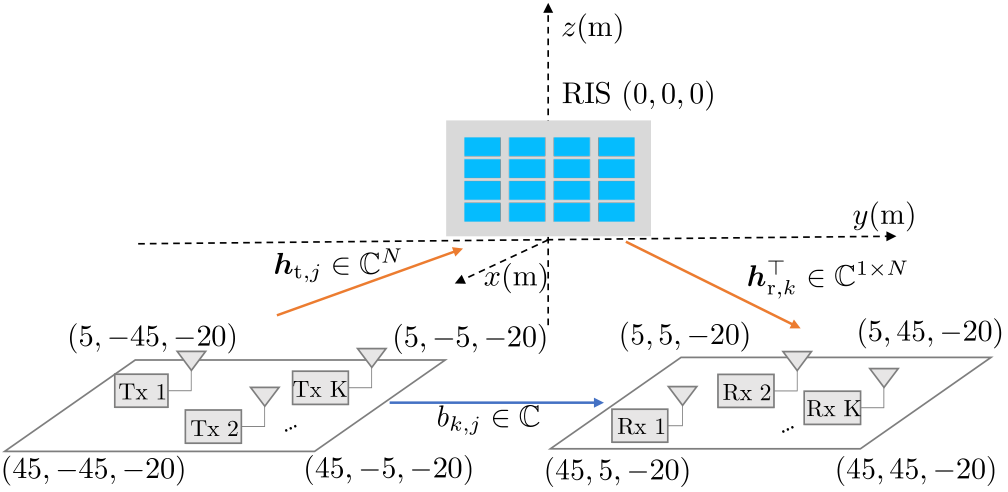
Fig. 1 shows the channel model with a blocked direct path. Let denote the channel between the transmitter and the RIS, and denote the channel between the RIS and the receiver . The reflection coefficients of the RIS are denoted by , where is the phase shift of the -th element of the RIS. Each transmitter sends a transmit symbol . All transmissions share the same time and frequency resource. Each receiver receives a reflected signal through the RIS, as given by
| (1) |
where
| (2) |
is the cascaded channel from transmitter to receiver , and is the additive Gaussian noise at receiver . The achievable rate of the -th link can now be expressed as
| (3) |
where is the fixed transmit power level of the -th link, i.e., .
The RIS reflection coefficients can be reconfigured based on the channel state information (CSI) for the purpose of maximizing a network utility function, e.g., the sum rate or the minimum rate across all the transceiver pairs. To this end, this paper assumes that the RIS can be configured by a centralized controller that can collect the CSI of all the links. The CSI can be estimated through a pilot phase (e.g., see [17, 18, 7]). In this paper, we assume that the CSI is perfectly known in order to investigate the system performance that can be achieved by optimizing the reflection coefficients at the RIS.
III Interference Nulling Capability of RIS
Assuming for now the channel model (II) in which all the signals go through the reflective path, we begin by investigating the feasibility of tuning the phase shifts at the RIS to completely null all the interference. Specifically, we seek to design the RIS reflection coefficients such that the following interference nulling conditions are satisfied:
| (4a) | ||||
| (4b) | ||||
| (4c) | ||||
The conditions in (4a) and (4b) guarantee that the powers of the desired signals are greater than zero and that all the interference signals are nulled out completely. In this case, the achievable rate of the -th transceiver pair is
| (5) |
and the degree of freedom of the link is
| (6) |
Thus, the overall -user interference channel achieves DoF.
Note that since the channel realizations are random, we can assume that with high probability, none of the effective desired channels are in the subspace spanned by the effective interfering channels . Otherwise, there is no solution to the interference nulling conditions (4a)-(4b). Since the effective channels are random vectors in , this is true with high probability as long as .
III-A Feasibility of Interference Nulling
The interference nulling is said to be feasible if there exists a vector such that the conditions in (4) are met. We also call the feasible solution a zero-forcing solution since it nulls all the interference. Given that the channel realizations are random, the condition (4a) typically holds with high probability. Thus, the rest of the paper focuses on conditions (4b) and (4c).
If the complex variables ’s are treated as unconstrained variables, then since the condition in (4b) involves complex linear equations and complex variable ’s, we simply need to ensure that (4b) has a solution. This would be the case if the RIS is active, i.e., it has both amplitude and phase control. But, the problem with passive lossless RIS is more complicated due to the unit modulus constraint (4c). If we count the number of real equations and the number of real variables in (4b) and (4c), there are nonlinear equations and real variables (i.e., phase shift ’s at the RIS), so intuitively we would need to ensure the existence of a feasible solution to (4b) and (4c).
To establish the above result rigorously is however not easy, because the equations are nonlinear. Further, even if we establish the existence of a zero-forcing solution to (4), it can be challenging to actually find the solution with low complexity. In Section IV, we propose a computationally efficient alternating projection algorithm, which is capable of finding a zero-forcing solution if is slightly larger than . Before presenting the alternating projection algorithm, we first provide the following theoretical result which shows that if the channels have a line-of-sight, then a sufficient condition for the feasibility of (4) can be established, i.e., zero-forcing solution exists for sufficiently large .
III-B A Sufficient Condition for Feasibility
When the channels between the users and the RIS follow a line-of-sight model and the RIS elements are arranged as a rectangular array as in a typical implementation, it is possible to establish a sufficient condition for zero-forcing that shows the conditions in (4) are feasible if the number of RIS elements exceeds some finite value that depends only on .
Consider an uniform rectangular array RIS with elements per row (horizontal direction) and elements per column (vertical direction). Let , denote the azimuth angle and the elevation angle of arrival, respectively. The -th element of the RIS array response vector can be written as [19]
| (7) |
where and are the horizontal and vertical spacings, and and denote the horizontal index and vertical index of element , respectively. The channel vector between the user and the RIS can then be written as
| (8) |
where is the path-loss between the user and the RIS, and and are the corresponding azimuth and elevation angles.
To find a sufficient condition for interference nulling, we make use of the following key lemma, which characterizes the properties of unimodular coefficient polynomials on the complex unit circle [20].
Lemma 1 ([20])
Given on the complex unit circle , there exists a polynomial of degree with unit modulus coefficients such that the points are the only zeros of on .
We establish the following sufficient condition for interference nulling for the line-of-sight channel model.
Theorem 1
Proof:
We begin with the case , which corresponds to the uniform linear array case. In this case, the channel between the RIS and transmitter can be written as
| (9) |
and the channel between the RIS and receiver can be written as
| (10) |
Thus, we have
| (11a) | ||||
| (11b) | ||||
where .
Let be a polynomial of degree with unit modulus coefficients as follows:
| (12) |
where . The interference nulling conditions in (4a), (4b), and (4c) become
| (13a) | ||||
| (13b) | ||||
which transform the original interference nulling problem to the problem of finding a polynomial as in (12) such that ’s are the roots, while the polynomial does not vanish at ’s. By Lemma 1, we know such a polynomial exists if .
To generalize the above result to the rectangular array case with , we make the argument that a rectangular uniform array can be viewed as columns of the uniformly linear array of size . Thus, if we set all the columns of the RIS to have the same reflection coefficients that null all the interference, which can be achieved if , the entire rectangular array would also achieve the interference nulling condition. Mathematically, this means that the same reflection coefficients are used times to produce a zero-forcing solution for all sub-vectors of as in (7).
Finally, if we exchange the roles of and , it is easily seen that the interference nulling conditions are also achievable if . This completes the proof. ∎
In Theorem 1, the number of RIS elements needs to scale exponentially with the number of transceiver pairs in order to ensure feasibility for zero-forcing. But, this is only a sufficient condition. In the next section, we develop practical algorithms that can find feasible solutions with high probability if the number of RIS elements is only slightly larger than , which is much smaller than the value required in Theorem 1.
We remark that the line-of-sight assumption on the channel model is made in Theorem 1 in order to prove the mathematical result. The algorithmic developments in the rest of the paper do not assume the line-of-sight channel model. Further, the algorithms can be extended to the case where the direct paths are not blocked.
IV Alternating Projection Algorithm for Interference Nulling
We now focus on the numerical algorithm for finding a zero-forcing solution in (4). Specifically, we focus on the interference nulling condition and formulate the following feasibility problem:
| (14a) | ||||||
| (14b) | ||||||
| (14c) | ||||||
For ease of presentation, we define the matrices and as:
| (15a) | ||||
| (15b) | ||||
where contains all the interference channels to the -th receiver and contains all the interference channels of all the transceiver pairs.
Then, (14) can be rewritten more compactly as
| (16a) | ||||||
| (16b) | ||||||
| (16c) | ||||||
This is a nonconvex optimization problem due to the unit modulus constraints, and is in general not easy to solve. In the following, we propose an efficient alternating projection method for solving (16).
IV-A Alternating Projection Method
We begin by defining the following two constraint sets
| (17a) | ||||
| (17b) | ||||
and rewrite problem (16) equivalently as
| (18) | ||||||
To find a point in the intersection of and , the alternating projection algorithm starts with an initial , then alternatively projects onto and as follows:
| (19a) | ||||
| (19b) | ||||
Here, the projection operation is defined as the point in the set that has the minimum Euclidean distance to , which can be obtained by solving the following problem
| (20) | ||||||
Fortunately, the projections to the sets and have simple analytical expressions, as given by
| (21a) | ||||
| (21b) | ||||
In (21a) the channel matrix is assumed to be full column rank (otherwise the matrix can be replaced by a new matrix constructed from the basis of the column space of ). In (21b), if some elements of the vector are zero, these elements can be projected to any random point on the complex unit circle. The alternating projection algorithm for solving problem (18) is summarized in Algorithm 1.
for do
if stopping criterion is satisfied then
IV-B Initialization
A simple way to initialize the alternating projection algorithm is to generate a random unit modulus vector , with i.i.d. uniform random phases in . However, the alternating projection algorithm only nulls the interference among all the transceiver pairs; it makes no attempt to maximize the received powers between the intended transceiver pairs. We point out here that since it is desirable to seek a zero-forcing solution that can also maximize the receive powers of the intended signals, instead of random initialization, the following initialization point could lead to better performance.
The sum power of the intended signals across all the links can be written as
| (22) |
where , and is subject to the unit modulus constraints. If we relax the unit modulus constraints to , then the sum of intended signal powers (22) is maximized by the eigenvector associated with the largest eigenvalue of the matrix . Experimentally, using as an initial point, followed by a projection to the unit modulus constraint set by (21b), is found to achieve higher sum rate as compared to random initialization. This is shown in the numerical simulation results in Section VII.
IV-C Convergence Analysis
The convergence of the alternating projection algorithm would have been easy to establish if and were convex sets. But in our setting, is the complex unit circle, which is not convex. Further, the projection operation onto may not be unique (the non-uniqueness occurs when has a zero component). So in general, even the local convergence of the alternating projection algorithm is not trivial to establish. This section presents a convergence analysis of the proposed algorithm, which is based on the following mathematical definitions.
Definition 1 (Semialgebraic set)
A set is a semialgebraic set if there exists a finite number of real polynomial functions and such that
| (23) |
Definition 2 (Prox-regular [21])
A set is prox-regular at a point if the projection mapping is single-valued around .
The semialgebraic property of the sets gives nice intersection geometry between the two sets, which is called separable intersection in [22]. Prox-regular property gives nice local geometry properties for the individual set [22]. The geometry of the intersection of the two sets and the regularity of individual sets play a critical role in deriving local convergence guarantee for the alternating projection algorithm. We refer to [23] for a detailed discussion on the local convergence theorem of the alternating projection algorithm. The following local convergence theorem for general semialgebraic sets is taken from [22].
Lemma 2 (Local convergence for semialgebraic sets [22, Corollary 8 and Corollary 3])
We now state the local convergence theorem for the proposed alternating projection method in Algorithm 1.
Theorem 2
Proof:
The set can be equivalently written as
| (24) |
where
| (25) |
which is a representation of the form (23). Hence, is a semialgebraic set. The set can be equivalently written as
| (26) |
Hence, is also a semialgebraic set. Since is a convex set, the projection onto from any point is single valued. is therefore prox-regular at the point . The proof then follows from Lemma 2. ∎
IV-D Discussions on Global Convergence Guarantee
Theorem 2 establishes a local convergence guarantee for the alternating projection algorithm. In general, it is difficult to establish global convergence guarantee from any initial starting point for alternating projection to nonconvex sets. However, it is observed in simulations that the proposed alternating projection algorithm always converges linearly to a feasible zero-forcing solution from any random initial point. To provide some intuitions about the convergence behavior, we discuss some conditions to guarantee the convergence of the alternating projection algorithm for general nonconvex sets. Specifically, the convergence of alternating projection algorithm for nonconvex sets can be established if and satisfy the following assumption [24, Theorem 1].
Assumption 1 ([24])
Let and be any two closed semialgebraic sets, and let be the sequence of iterates generated by the alternating projection method. Assume that the sequence is bounded and there exist subsets and and such that and for all . Furthermore, we assume that the sets , and subsets , obey the following properties:
- •
Three-point property: There exists a nonnegative function with such that for all we have and for all , , we have
(27) - •
Local contraction property of with respect to : There exist and such that
(28) for all .
If Assumption 1 holds, the sequence generated by the alternating projection algorithm can be shown to converge to a critical point of the following problem [24]:
| (29) |
where if , and otherwise . This is an equivalent formulation of the problem (18).
It is clear that the local contraction property of with respect to always holds with since is a convex set. With respect to the three-point property, let , , we have
| (30a) | |||||
| (30b) | |||||
| (30c) | |||||
| (30d) | |||||
| (30e) | |||||
where to write (30b) we use , from which we can obtain . From (30e), the three-point property of is satisfied as long as is bounded away from 0, in which case the convergence guarantee can then be established. However, requiring that each element of is bounded away from zero for for some is a strong assumption. Nevertheless, it is uncommon for to have near-zero elements; this may explain why the proposed alternating projection algorithm always converges from any random initial point in numerical simulations.
IV-E Complexity Analysis
At each iteration, the time complexity of the proposed alternating projection algorithm is dominated by the projection onto the set in (21a). Since we need to compute (21a) at each iteration, we can compute at the first iteration and reuse its value for subsequent iterations. The complexity of computing is for general dense matrix . Thus, the total computational complexity is , where is the number of iterations needed to converge. If the alternating projection algorithm is initialized by the eigenvalue decomposition based method, additional time complexity is needed for computing the eigenvector associated with the largest eigenvalue [25].
V Network Utility Maximization
The alternating projection algorithm seeks a zero-forcing solution to null the interference completely. However, except through the initialization method as proposed in subsection IV-B, the iterates of alternating projection do not attempt to maximize the desired signal power. Thus, although the RIS is configured to suppress interference, the zero-forcing solution does not necessarily maximize network utility. In this section, we consider the numerical optimization of network utility functions in practical network settings.
V-A Sum-Rate Maximization Algorithm
Consider first the sum-rate maximization problem for the RIS system. We propose the following two-stage algorithm that utilizes the zero-forcing solution to maximize the sum rate in a -user interference channel. First, we run the alternating projection algorithm for the interference nulling problem. In the second stage, the solution found by the alternating projection algorithm is used as an initial point for the subsequent iterative algorithm for maximizing the network sum rate. The second stage uses the RCG method in order to accommodate the unit modulus constraints. The unit modulus constraints form a Riemannian manifold [26, 27].
More specifically, the sum-rate maximization problem is formulated as follows:
| (31) | ||||
The above sum-rate maximization problem (31) is nonconvex due to the nonconvex objective function and nonconvex unit modulus constraints. Since the objective function of problem (31) is continuous and differentiable, one straightforward approach is to use the projected gradient method. But instead of taking the Euclidean gradient, a better approach is to use the Riemannian gradient, which is formed by projecting the Euclidean gradient onto the tangent space of the complex circle manifold formed by the unit modulus constraints. Further, to speed up convergence, the conjugate Riemannian gradient may be used. This results in the RCG method, as proposed in [26, 27].
The RCG method consists of three steps. First, the Euclidean gradient at the point is computed as
| (32) |
where
| (33) |
By projecting the Euclidean gradient onto the tangent space of the complex unit circle, we obtain the Riemannian gradient as follows [27, 5]:
| (34) |
where
| (35) |
with denoting the element-wise product.
Second, given the Riemannian gradient, the search direction is updated by the conjugate gradient method as follows:
| (36) |
where is the conjugate gradient update parameter, and is the previous search direction.
Finally, to keep the updated point on the manifold, we need a retraction operation to project the point onto the manifold as follows:
| (37) |
where is the Armijo step size.
Compute search direction by (36)
Update by (37)
if stopping criterion is satisfied then
The overall algorithm is summarized as Algorithm 2. The RCG method is guaranteed to converge to a stationary point of the problem (31) [28]. The main advantage of using the zero-forcing solution as the initial point is that it helps the RCG method avoid undesirable local maxima. The numerical results in Section VII show that such a two-stage optimization algorithm achieves significantly better performance as compared to methods with random initializations.
V-B Minimum-Rate Maximization Algorithm
The sum-rate objective function does not take fairness into consideration. In this section, we investigate how to design the RIS system in order to maximize the minimum rate over all links in a -user interference channel.
The minimum-rate maximization problem can be formulated as the following optimization problem:
| (38) | ||||
Compared with the sum-rate maximization problem (31), the objective function of the minimum rate maximization problem (38) is no longer smooth, so RCG or gradient-based methods cannot be directly applied. Existing methods in the literature include bisection or fractional programming with SDR [7, 8], or penalty method followed by SCA [9].
This paper proposes a subgradient projection method to solve the problem (38). This method is found to have good performance and has a complexity which is scalable even for large values of . We numerically show in Section VII that the subgradient method can outperform the SDR-based method considerably, and has complexity much lower than SCA.
A vector is a subgradient of the function if it is an element of the Fréchet subdifferential [29]. Next, we show that a subgradient of can be given as
| (39) |
where . The proof follows the proof technique from [30]. Since is compact, is finite for any and . Then there exists a constant such that . This implies is -smooth. Thus for all and for all , we have [31]
Let , we thus have
| (40) |
By rearranging the terms in (40) and taking for , we conclude that (39) is a subgradient of .
Given the subgradient (39), the projected subgradient method takes the following form:
| (41) |
where is the step size at the -th iteration. The step size of the projected subgradient method needs to be properly chosen to promote fast convergence. One example of step size selection is to choose the constant step size normalized by the norm of the subgradient [32], i.e.,
| (42) |
which is shown to achieve good performance in practice. Because the subgradient method cannot guarantee decrease in the objective functions for each iteration, we keep track of the best point found so far during the iterations.
Unlike the sum-rate maximization problem, the initialization by the zero-forcing solution does not have a significant impact for the performance of the minimum-rate maximization problem. This is because the minimum rate objective function typically has a bottleneck link, and it is only crucial to null the interference for the bottleneck link, but not the other links.
VI RIS System with Direct Paths Between the Transmitters and Receivers
So far, we have considered the system model where the direct paths between the transmitters and the receivers are blocked. However, the algorithms proposed in this paper are not limited to this scenario. In this section, we extend the proposed algorithms to the RIS systems with direct paths.
Let denote the direct channel between transmitter and receiver , the received signal model (II) can be rewritten as
| (43) |
In this case, the achievable rate of the -th link becomes
| (44) |
Similar to the interference nulling conditions in (4a), (4b), (4c), we can establish the interference nulling conditions for the case with direct paths as follows:
| (45a) | ||||
| (45b) | ||||
| (45c) | ||||
Accordingly, the problem (16) can be reformulated as that of finding a feasible solution to the following problem:
| (46) | ||||||
The proposed alternating projection algorithm can be readily applied to solve the above problem (46). Specifically, the set in (17a) becomes an affine set , and the projection to this affine set also has a closed-form solution [33]:
| (47) |
The other parts of the proposed alternating projection algorithm remain unchanged. The local convergence guarantee in Theorem 2 still holds since the new affine set remains convex.
We note that the strength of the direct channel affects the feasibility of the problem (46). For a zero-forcing solution to exist, it is necessary to have
| (48) |
otherwise even aligning the strength of all the cascaded channels, i.e., all the elements , cannot cancel out the interference caused by the direct channel . From (48), the value of depends on both the strength of the cascaded channel and the number of RIS elements . If the strength of the cascaded channel is relatively small, e.g., due to the large loss caused by the passive reflection [34], as compared to the direct channel , the number of RIS elements would need to be large in order to cancel the interference caused by both the direct and the reflection paths.
The algorithms developed for maximizing the sum rate or the minimum rate can be likewise extended to the case with direct paths by recomputing the gradients as
| (49) |
VII Simulation Results
In this section, we present numerical results to evaluate the performance of the proposed algorithms for optimizing the RIS system with different objective functions. We first evaluate the algorithm for the scenario without direct paths, then consider the scenario with direct links.
VII-A Simulation Setup
We consider a simulation setup as shown in Fig. 2. An RIS equipped with a uniform rectangular array is placed on the -plane at the coordinate in meters. The transmitters and the receivers are uniformly distributed in a rectangular area and respectively, and the -coordinates of all the users are set to be . The channel model between the RIS and the user is assumed to be Rician fading channel as in [35], which is modeled as
| (50) |
where is the path-loss from the RIS to the user , is the line-of-sight part and is the non-line-of-sight part. The path-loss in dB is modeled as where is the distance between the user and the RIS in meters. The line-of-sight channel is modeled as in (8), i.e., and the entries of the non-line-of-sight channel vector are modeled as i.i.d. standard Gaussian distributions, i.e., . The system bandwidth is MHz and the noise spectral density is dBm/Hz.
In Section VII-B to VII-D, we consider the scenario without the direct paths, i.e., . The scenario with the direct paths is considered in Section VII-E, where the model for the direct channels is described in detail.
| RIS location | |
|---|---|
| Tx location | |
| Rx location | |
| Path-loss for and | |
| Bandwidth | MHz |
| Noise power spectral density | dBm/Hz |
VII-B Interference Nulling Problem
For the interference nulling problem, to verify the effectiveness of the proposed alternating projection algorithm, we compare it to the following projected gradient method as a baseline.
VII-B1 Baseline Projected Gradient Method
The interference nulling problem (16) can also be formulated as follows:
| (51) | ||||||
where the sum of interference is minimized subject to the unit modulus constraint on . If the objective function of problem (51) is minimized to be zero, then we find a zero-forcing solution that nulls all the interference. The problem (51) can be solved by the projected gradient method [36], which has the following update rule:
| (52) | ||||
| (53) |
where is the step size at the -th iteration. The choice of an appropriate step size is crucial for the algorithm to converge. However, it is computationally expensive to identify the optimal step size that minimizes the objective function along the descent direction. A common practice is to select the step size by backtracking line search [37]. Specifically, let , and . We keep shrinking the step size by until .
We should note that the proposed alternating projection method is a parameter-free algorithm, while the projected gradient method needs to adjust its step size at each iteration.

VII-B2 Convergence Speed
We now provide simulations to evaluate the convergence rate of the proposed alternating projection method, i.e., Algorithm 1, as compared to the projected gradient method. In this experiment, the RIS consists of passive elements and serves transceiver pairs. We run independent random trials with different random initial points for the proposed alternating projection algorithm and the projected gradient method. The maximum interference-to-signal ratio (ISR) over the links is adopted as the performance metric. For the projected gradient method, the backtracking search parameters are set as and .
From Fig. 3, it can be observed that the alternating projection algorithm can decrease the maximum ISR to about dB within iterations for almost all the trials. However, the projected gradient method takes around iterations to reach this level of maximum ISR. We observe that the maximum ISR is not always monotonically decreasing at the beginning. This is because the alternating projection algorithm and the projected gradient method only attempt to reduce the interference, without regard to the power of the useful signals, so it does not necessarily result in a decrease in the maximum ISR. However, the maximum ISR eventually decreases almost linearly in later iterations.
VII-B3 Phase Transitions
To evaluate the performance of the proposed alternating projection algorithm for finding a zero-forcing solution, we also adopt the maximum ISR as the metric. We declare that an interference nulling solution is found if the maximum ISR across all transceiver pairs is below dB. We evaluate systems with ranging from to and ranging from to . The RIS is assumed to be a uniform linear array for convenience so that we can increase at a step size . For each setting of and , independent trials are conducted to estimate the interference nulling probability.
To evaluate the impact of different channel distributions on the performance, we also consider the sparse channel model and Rayleigh fading channel model. For the sparse channel model, , where the superscript denotes the -th path, with the number of path for the channels between the transmitters/receivers and the RIS. For the Rayleigh fading channel model, we have that for the channels between the transmitters/receivers and the RIS.
In Fig. 4(a), we plot the empirical success probability versus the number of RIS elements for the Rician channel model as in (50). We observe a phase transition phenomenon, i.e., for any fixed , the empirical interference nulling probability transitions sharply from to as exceeds a threshold. As increases, the phase transition location grows approximately as , implying that the interference can be completely nulled with high probability using the proposed alternating projection algorithm if is slightly greater than .
The phase transition location can be more precisely observed in Fig. 4(b). In Fig. 4(b), the points marked as “ success” refer to the points below which all the trials fail to find a zero-forcing solution. The points marked as “ success” refer to the points above which a zero-forcing solution can be found with empirical probability greater than . From Fig. 4(b), we can see the that “ success” lines coincide with the line , which implies that the is a necessary condition for the existence of a zero-forcing solution. It is also observed that if is only slightly larger than , the proposed alternating projection algorithm can already find a zero-forcing solution with high probability. Furthermore, the distribution of the channels does not affect the performance of the proposed alternating projection algorithm or the location of phase transition.
VII-C Sum-Rate Maximization
To demonstrate the efficiency of the proposed two-stage method for solving the sum-rate maximization problem (31), we compare the sum rate achieved by the following schemes:
- •
AP With Random Init.: The alternating projection algorithm for zero-forcing is initialized by a unit modulus vector with random phases.
- •
AP With Eigen Init.: The alternating projection algorithm for zero-forcing is initialized by the eigenvalue decomposition scheme proposed in Section IV-B.
- •
Random Init. + RCG: The RCG algorithm for sum-rate maximization is initialized by a unit modulus vector with random phases.
- •
AP With Random Init. + RCG: The RCG algorithm for sum-rate maximization is initialized by a zero-forcing solution obtained by the alternating projection algorithm, which is itself initialized by a unit modulus vector with random phases.
- •
AP With Eigen Init. + RCG: The RCG algorithm for sum-rate maximization is initialized by a zero-forcing solution obtained by the alternating projection algorithm, which is itself initialized by the eigenvalue decomposition scheme proposed in Section IV-B.
Moreover, we compare the performance of directly using RCG on the objective function to an alternative approach of first reformulating the sum-rate maximization problem using a closed-form fractional programming (FP) technique [38], then solving the reformulated problem by block coordinate descend (BCD). In each step of the BCD algorithm, the reflection coefficients at the RIS can be updated by either SCA [5] or RCG. The zero-forcing solution obtained by alternating projection can also be used as the initialization point in this case. Specifically, the following schemes are compared:
- •
Random Init. + FP With SCA: The FP based algorithm with SCA is initialized by a unit modulus vector with random phases.
- •
Random Init. + FP With RCG: The FP based algorithm with RCG is initialized by a unit modulus vector with random phases.
- •
AP With Eigen Init. + FP With SCA: The FP based algorithm with SCA is initialized by the zero-forcing solution obtained by the proposed alternating projection algorithm with the eigenvalue decomposition initialization scheme.
- •
AP With Eigen Init. + FP With RCG: The FP based algorithm with RCG is initialized by the zero-forcing solution obtained by the proposed alternating projection algorithm with the eigenvalue decomposition initialization scheme.
The simulation results of the above different approaches are shown in Fig. 5, where each point is averaged over independent channel realizations. For the experiments in Fig. 5(a), we set the number of RIS elements and the number of transceiver pairs respectively to and . As can be seen from Fig. 5(a), with the random initialization, the sum rates achieved by the RCG method and the FP based method increase with the transmit power initially with FP outperforming RCG, but their performances gradually saturate as the transmit power increases. On the other hand, although the sum rates achieved by the zero-forcing solutions are lower at low SNR, their performances increase almost linearly as the transmit power increases, and eventually catch up with the RCG or FP algorithms at high SNR. Between the two zero-forcing schemes, using the eigenvalue decomposition based initialization significantly outperforms random initialization. But the best performance is achieved if the RCG or the FP based method is initialized by the zero-forcing solution. Such a two-stage optimization scheme can achieve much better performance than using either the zero-forcing solution directly or the RCG or FP based method with random initialization.
We note that although the FP based algorithm outperforms RCG if random initialization is used, their performances are almost indistinguishable when the zero-forcing solution is used as the initialization. In terms of complexity, using the RCG algorithm directly on the sum-rate objective has a lower complexity than FP, because an iterative algorithm (SCA or RCG) is needed to update the reflection coefficients at each iteration of the BCD algorithm after the FP step. Thus, using the RCG algorithm with zero-forcing initialization is overall the best approach.
In Fig. 5(b), we plot the sum rate versus the number of RIS elements for fixed dBm transmit power with the number of transceivers . The RIS consists of elements in the horizontal direction. From Fig. 5(b), we can observe that RCG with the zero-forcing solution as the initial point consistently achieves the best performance as compared to the other schemes. We observe a significant increase in the sum rate for the alternating projection algorithm when changes from to . This is because is around the phase transition point when (see Fig. 4(a)). It is interesting to observe that RCG with the solution returned by the alternating projection algorithm as the initial point can outperform RCG with a random initialization scheme even if the interference cannot be suppressed completely.
VII-D Minimum-Rate Maximization
To verify the effectiveness of the proposed subgradient method for minimum-rate maximization, we compare its performance with the SDR-based bisection search method [8] and the SCA based approach [9]. In the SDR approach, the optimization variable is lifted to the space of matrix variables by defining a matrix variable . This eliminates the nonconvex unit modulus constraints on . Semidefinite programming can then be applied in order to find an optimal . If SDR returns a matrix with a rank greater than one, we use Gaussian randomization (with 1000 samples in this case) to obtain a solution . In the SCA based algorithm, the unit modulus constraint of problem (38) is enforced by a penalty term in the objective function [9], then the objective function is approximated successively by a convex function and the resulting optimization problem is solved in each iteration. In the simulations, we use the CVX [39] software with SDPT3 solver to solve this convex optimization problem. For the proposed subgradient method, we set the maximum number of iterations to be and stop the algorithm if there is no improvement on the objective function in consecutive iterations.
In Fig. 6, we plot the average minimum rate versus the transmit power. The number of transceiver pairs is set to . We consider two scenarios where the number of RIS elements is and . In the former case, as can be observed from Fig. 4(b), the interference cannot be completely nulled. In the latter case, we can find a zero-forcing solution using the alternating projection algorithm with high probability.
From Fig. 6, it is clear that zero-forcing by itself does not produce a good minimum rate. We also observe that both the SCA and the subgradient method outperforms the SDR based bisection search method significantly. Furthermore, the performance gain of the SCA and the subgradient method over the SDR-based bisection search method increases as increases from to . This is because the SDR approach does not necessarily find a rank-one solution, especially for large values of . At high SNR, the SCA algorithm is slightly better than the subgradient method. However, the SCA method needs to solve a convex optimization problem at each iteration. This leads to an order of magnitude higher complexity than the running time of the subgradient method. Thus, the subgradient method is the best choice from a complexity-performance tradeoff perspective.
VII-E RIS System with Transmitter-Receiver Direct Paths
In this subsection, we evaluate the performance of the proposed algorithms on scenarios with direct paths between the transmitters and the receivers. The direct channels are modeled as Rayleigh fading channels, i.e.,
| (54) |
where is the path-loss and .
To see the influence of the strength of the direct channel on the feasibility of zero-forcing solutions, we set the path-loss values of the direct links to be . In comparison, the average path-loss of the cascaded link is about . The number of transceiver pairs is , and again the RIS is assumed to be a linear array for convenience. From Fig. 7(a), we can see that the phase transition location does not change if the strength of the direct path is relatively small. But, the phase transition location moves toward higher values of if the strength of the direct path exceeds some threshold. This implies that more elements at the RIS are needed to null all the interference if the strength of the direct path exceeds some threshold value.
To characterize this phenomenon more precisely, let denote the maximum ratio between the strength of the direct path and the corresponding norm of the cascaded channels, defined as follows:
| (55) |
In the next experiment, the number of transceiver pairs is . By varying the path-loss of the direct paths to be , we record the average over channel realizations and the corresponding empirical probability of finding a zero-forcing solution. In Fig. 7(b), we plot the empirical interference nulling probability versus the average . It can be seen that the probability of finding a zero-forcing solution decreases as the value of the average increases. However, we can increase the number of elements at the RIS to compensate.
Finally, we evaluate the performance of the proposed algorithm for the sum-rate maximization problem in the presence of the direct paths. The number of RIS elements is , and the number of transceiver pairs is . The path-loss of the direct path is fixed to be . As can be seen from Fig. 7(b), we observe a similar phenomenon as the case without direct paths in Fig. 5(a), e.g., RCG with zero-forcing solution as the initialization achieves the best sum-rate performance. This shows that the proposed algorithm can be readily applied to scenarios with direct channels between the transmitters and the receivers.
VIII Conclusion
This paper investigates an RIS-enabled multiple-access environment modeled as a -user interference channel, where transceiver pairs communicate through reflection by the RIS. We show that it is possible to configure the reflective coefficients of the RIS to completely null interference and to achieve DoF, if the number of elements at the RIS is sufficiently large. Specifically, for the line-of-sight channel model without the direct paths, we show that there exists a solution to achieve DoF if the number of RIS elements exceeds some finite value that depends only on . Further, we propose an alternating projection algorithm with local convergence guarantee to find the zero-forcing solution for any arbitrary channel realizations. Numerical results demonstrate that the proposed alternating projection algorithm can achieve interference nulling if the number of RIS elements is slightly larger than .
This paper also proposes an efficient two-stage scheme to maximize the network sum rate. We show experimentally that using the zero-forcing solution obtained by the alternating projection algorithm as the initial point for the subsequent RCG method can significantly improve the optimization performance as compared to random initialization. For the problem of maximizing the minimum rate, we propose a subgradient projection method which is scalable to large . In all, the results of this paper demonstrate the considerable capability of the RIS for interference nulling in an RIS-assisted multiuser communications environment.
References
- [1] V. R. Cadambe and S. A. Jafar, “Interference alignment and degrees of freedom of the -user interference channel,” IEEE Trans. Inf. Theory, vol. 54, no. 8, pp. 3425–3441, Aug. 2008.
- [2] M. Di Renzo, A. Zappone, M. Debbah, M.-S. Alouini, C. Yuen, J. de Rosny, and S. Tretyakov, “Smart radio environments empowered by reconfigurable intelligent surfaces: How it works, state of research, and road ahead,” IEEE J. Sel. Areas Commun., vol. 38, no. 11, pp. 2450 –2525, July 2019.
- [3] C. Huang, A. Zappone, G. C. Alexandropoulos, M. Debbah, and C. Yuen, “Reconfigurable intelligent surfaces for energy efficiency in wireless communication,” IEEE Trans. Wireless Commun., vol. 18, no. 8, pp. 4157–4170, Aug. 2019.
- [4] Q. Wu and R. Zhang, “Intelligent reflecting surface enhanced wireless network via joint active and passive beamforming,” IEEE Trans. Wireless Commun., vol. 18, no. 11, pp. 5394–5409, Nov. 2019.
- [5] H. Guo, Y.-C. Liang, J. Chen, and E. G. Larsson, “Weighted sum-rate maximization for reconfigurable intelligent surface aided wireless networks,” IEEE Trans. Wireless Commun., vol. 19, no. 5, pp. 3064–3076, May 2020.
- [6] S. Zhang and R. Zhang, “Capacity characterization for intelligent reflecting surface aided MIMO communication,” IEEE J. Sel. Areas Commun., vol. 38, no. 8, pp. 1823–1838, Aug. 2020.
- [7] H. Alwazani, A. Kammoun, A. Chaaban, M. Debbah, and M.-S. Alouini, “Intelligent reflecting surface-assisted multi-user MISO communication: Channel estimation and beamforming design,” IEEE Open J. Commun. Soc., vol. 1, pp. 661–680, May 2020.
- [8] H. Xie, J. Xu, and Y.-F. Liu, “Max-min fairness in IRS-aided multi-cell MISO systems with joint transmit and reflective beamforming,” IEEE Trans. Wireless Commun., vol. 20, no. 2, pp. 1379–1393, Feb. 2021.
- [9] H. Yu, H. D. Tuan, A. A. Nasir, T. Q. Duong, and H. V. Poor, “Joint design of reconfigurable intelligent surfaces and transmit beamforming under proper and improper Gaussian signaling,” IEEE J. Sel. Areas Commun., vol. 38, no. 11, pp. 2589–2603, Nov. 2020.
- [10] X. Yu, D. Xu, Y. Sun, D. W. K. Ng, and R. Schober, “Robust and secure wireless communications via intelligent reflecting surfaces,” IEEE J. Sel. Areas Commun., vol. 38, no. 11, pp. 2637–2652, Nov. 2020.
- [11] W. Zhao, S.-H. Lee, and A. Khisti, “Phase-only zero forcing for secure communication with multiple antennas,” IEEE J. Sel. Topics Signal Process., vol. 10, no. 8, pp. 1334–1345, Dec. 2016.
- [12] A. H. A. Bafghi, V. Jamali, M. Nasiri-Kenari, and R. Schober, “Degrees of freedom of the -user interference channel in the presence of intelligent reflecting surfaces,” 2020. [Online]. Available: https://arxiv.org/abs/2012.13787
- [13] M. Fu, Y. Zhou, and Y. Shi, “Reconfigurable intelligent surface for interference alignment in MIMO device-to-device networks,” in IEEE Inter. Conf. Commun. (ICC) Workshops, 2021, pp. 1–6.
- [14] Y. Chen, B. Ai, H. Zhang, Y. Niu, L. Song, Z. Han, and H. Vincent Poor, “Reconfigurable intelligent surface assisted device-to-device communications,” IEEE Trans. Wireless Commun., vol. 20, no. 5, pp. 2792–2804, May 2021.
- [15] Z. Ji and Z. Qin, “Reconfigurable intelligent surface enhanced device-to-device communications,” in IEEE Global Commun. Conf. (GLOBECOM), Dec. 2020, pp. 1–6.
- [16] A. Abrardo, D. Dardari, M. Di Renzo, and X. Qian, “MIMO interference channels assisted by reconfigurable intelligent surfaces: Mutual coupling aware sum-rate optimization based on a mutual impedance channel model,” IEEE Wireless Commun. Lett., vol. 10, no. 12, pp. 2624–2628, Dec. 2021.
- [17] J. Chen, Y.-C. Liang, H. V. Cheng, and W. Yu, “Channel estimation for reconfigurable intelligent surface aided multi-user MIMO systems,” 2019, accepted in IEEE Trans. Wireless Commun. [Online]. Available: https://arxiv.org/abs/1912.03619
- [18] Z. Wang, L. Liu, and S. Cui, “Channel estimation for intelligent reflecting surface assisted multiuser communications: Framework, algorithms, and analysis,” IEEE Trans. Wireless Commun., vol. 19, no. 10, pp. 6607–6620, Oct. 2020.
- [19] E. Björnson and L. Sanguinetti, “Rayleigh fading modeling and channel hardening for reconfigurable intelligent surfaces,” IEEE Wireless Commun. Lett., Apr. 2020.
- [20] D. J. Newman and A. Giroux, “Properties on the unit circle of polynomials with unimodular coefficients,” Proc. Amer. Math. Soc., vol. 109, no. 1, pp. 113–116, 1990.
- [21] A. S. Lewis, D. R. Luke, and J. Malick, “Local linear convergence for alternating and averaged nonconvex projections,” Found. Comput. Math., vol. 9, no. 4, pp. 485–513, Nov. 2009.
- [22] D. Noll and A. Rondepierre, “On local convergence of the method of alternating projections,” Found. Comput. Math., vol. 16, no. 2, pp. 425–455, 2016.
- [23] A. Y. Kruger, D. R. Luke, and N. H. Thao, “Set regularities and feasibility problems,” Math. Program., vol. 168, no. 1, pp. 279–311, June 2018.
- [24] Z. Zhu and X. Li, “Convergence analysis of alternating projection method for nonconvex sets,” 2018. [Online]. Available: https://arxiv.org/abs/1802.03889
- [25] L. N. Trefethen and D. Bau III, Numerical linear algebra. SIAM, 1997, vol. 50.
- [26] X. Yu, J.-C. Shen, J. Zhang, and K. B. Letaief, “Alternating minimization algorithms for hybrid precoding in millimeter wave MIMO systems,” IEEE J. Sel. Topics Signal Process., vol. 10, no. 3, pp. 485–500, April 2016.
- [27] X. Yu, D. Xu, and R. Schober, “MISO wireless communication systems via intelligent reflecting surfaces,” in IEEE/CIC International Conf. Commun. China (ICCC), 2019, pp. 735–740.
- [28] P.-A. Absil, R. Mahony, and R. Sepulchre, Optimization algorithms on matrix manifolds. Princeton University Press, 2009.
- [29] R. T. Rockafellar and R. J.-B. Wets, Variational analysis. Springer Sci. Bus. Media, 2009, vol. 317.
- [30] C. Zhang, M. Dong, and B. Liang, “Fast first-order algorithm for large-scale max-min fair multi-group multicast beamforming,” 2021. [Online]. Available: https://arxiv.org/abs/2107.07540
- [31] A. Beck, First-order methods in optimization. SIAM, 2017.
- [32] S. Boyd, L. Xiao, and A. Mutapcic, “Subgradient methods,” Lecture notes of EE392o, Stanford University, Autumn Quarter, vol. 2004, pp. 2004–2005, 2003.
- [33] N. Parikh and S. Boyd, “Proximal algorithms,” Found. Trends Optim., vol. 1, no. 3, pp. 127–239, 2014.
- [34] M. Najafi, V. Jamali, R. Schober, and H. V. Poor, “Physics-based modeling and scalable optimization of large intelligent reflecting surfaces,” IEEE Trans. Commun., vol. 69, no. 4, pp. 2673–2691, April 2021.
- [35] T. Jiang, H. V. Cheng, and W. Yu, “Learning to reflect and to beamform for intelligent reflecting surface with implicit channel estimation,” IEEE J. Sel. Areas Commun., vol. 39, no. 7, pp. 1931–1945, Jul. 2021.
- [36] J. Tranter, N. D. Sidiropoulos, X. Fu, and A. Swami, “Fast unit-modulus least squares with applications in beamforming,” IEEE Trans. Signal Process., vol. 65, no. 11, pp. 2875–2887, June 2017.
- [37] S. Boyd, S. P. Boyd, and L. Vandenberghe, Convex optimization. Cambridge university press, 2004.
- [38] K. Shen and W. Yu, “Fractional programming for communication systems—Part II: Uplink scheduling via matching,” IEEE Trans. Signal Process., vol. 66, no. 10, pp. 2631–2644, May 2018.
- [39] M. Grant and S. Boyd, “CVX: Matlab software for disciplined convex programming, version 2.1,” http://cvxr.com/cvx, Mar. 2014.