Practical Fixed-Parameter Algorithms for Defending Active Directory Style Attack Graphs
Abstract
Active Directory is the default security management system for Windows domain networks. We study the shortest path edge interdiction problem for defending Active Directory style attack graphs. The problem is formulated as a Stackelberg game between one defender and one attacker. The attack graph contains one destination node and multiple entry nodes. The attacker’s entry node is chosen by nature. The defender chooses to block a set of edges limited by his budget. The attacker then picks the shortest unblocked attack path. The defender aims to maximize the expected shortest path length for the attacker, where the expectation is taken over entry nodes.
We observe that practical Active Directory attack graphs have small maximum attack path lengths and are structurally close to trees. We first show that even if the maximum attack path length is a constant, the problem is still -hard with respect to the defender’s budget. Having a small maximum attack path length and a small budget is not enough to design fixed-parameter algorithms. If we further assume that the number of entry nodes is small, then we derive a fixed-parameter tractable algorithm.
We then propose two other fixed-parameter algorithms by exploiting the tree-like features. One is based on tree decomposition and requires a small tree width. The other assumes a small number of splitting nodes (nodes with multiple out-going edges). Finally, the last algorithm is converted into a graph convolutional neural network based heuristic, which scales to larger graphs with more splitting nodes.
1 Introduction
Cyber attack graphs model the chain of events (conceptual or physical) that lead to successful cyber attacks. Despite its popularity in both academia and industry, there is not a canonical definition of cyber attack graphs. Lallie et al. 2020 surveyed over attack graphs/trees studied in literature, and discovered over different self-nominated definitions of attack graphs/trees.
For industry practitioners, there is one attack graph model that stands out and finds its place in many practitioners’ toolkit, which is the Active Directory attack graph. Microsoft Active Directory is the default security management system for Windows domain networks, which has a dominant market share among large organisations worldwide. Due to its popularity, Active Directory has been a focused cyber attack target. An Active Directory environment naturally describes an attack graph, where the nodes represent accounts, computers, security groups, etc. A directed edge from node A to B represents that an attacker can reach from A to B via existing accesses or known exploits. There are a number of software tools for analysing/visualising Active Directory attack graphs. Among these tools, BloodHound11 1 https://github.com/BloodHoundAD/BloodHound is the most influential. Motivated by Dunagan et al. 2009, BloodHound models the identity snowball attack under Active Directory. Typically, an identity snowball attack starts when an attacker gains initial access to the internal network. The attacker starts from a low-privilege user account (often obtained via phishing emails). The attacker then moves from low-privilege nodes to high-privilege nodes (i.e., account A computer B account C). The goal of the attacker is to reach the highest-privilege account, called the Domain Admin DA. The core functionality of BloodHound is to automatically generate the shortest attack path from the attacker’s entry node to DA, where the distance is defined as the number of hops. Following the shortest attack path implies less time spent on the attack and less chance of failure. Before the invention of BloodHound, attackers used to explore aimlessly in the internal network hoping to discover a privilege escalation pathway. Dunagan et al. 2009 briefly described a heuristic edge blocking algorithm. The aim is to block a small number of edges to cut the attack graph into multiple disconnected regions, which essentially removes the attack paths from most entry nodes.
We derive optimal edge blocking policies. The defender can assign different utilities on attack paths of different lengths. That is, maximizing the number of attack paths cut is a special case of our model. We adopt a two-player Bayesian Stackelberg game Paruchuri et al. 2008 setup with pure strategies only. In our game, the defender (leader) has a limited budget for blocking edges. Not all edges are blockable. The attacker’s type is characterized by his entry node. In practise, the entry account is often from a phishing attack victim. Therefore, we assume that the attacker’s entry node is drawn randomly by nature from a set of entry nodes (i.e., users whose emails are listed on the organisation’s website). The attacker is the follower in the Stackelberg game. That is, the attacker is aware of which edges have been blocked.22 2 In practise, the attacker can use a tool called SharpHound to scan the environment to obtain information on all edges. We assume that the attacker follows BloodHound’s advice and attacks via a shortest attack path. The defender aims to maximize the attacker’s expected shortest path length, where expectation is taken over all entry nodes.
When there is only one entry node, our model reduces to the well-studied shortest path edge interdiction problem (also called the most vital edges problem). Bar-noy et al. 1995 already showed that the problem is NP-hard. Nevertheless, this negative result does not rule out scalable algorithms for practical Active Directory attack graphs. We adopt parameterized complexity analysis and design fixed-parameter tractable (FPT) algorithms. Fixed-parameter algorithms allow us to solve some NP-hard problem instances efficiently and optimally, under the assumption that the problem instances are characterized by a few parameters that are small. For example, vertex cover is known to be NP-complete, but the question “whether there exists a vertex cover of size ” can be solved in , where is the number of nodes Chen et al. 2006. That is, if one’s goal is to solve vertex cover, and in one’s practical scenario is never too large, then the NP-completeness of vertex cover is irrelevant. Formally speaking, given problem instances with parameters , the computational problem is fixed-parameter tractable if we can design an algorithm with complexity . That is, the complexity is allowed to be exponential in the parameters, but it needs to be polynomial in the input size . This allows us to scale to large input sizes, as long as the parameters are small.
A natural question to ask is what should be the appropriate parameters for describing Active Directory attack graph instances. To answer this, let us consider the following attack graph. Figure 1 is a synthetic attack graph generated using BloodHound team’s synthetic database generator DBCreator.33 3 It should be noted that an organisation’s Active Directory attack graph is considered sensitive information. Our paper only references synthetic graphs generated using DBCreator. DBCreator generates a lot of details, such as a node’s operating system, department, real names. We only extract the topology. We make two observations. First, the maximum attack path length is small. Second, the graph looks like a tree. Our observation is not an artifact based upon DBCreator. It is considered a best practise for Active Directory to follow the organisation chart. For example, marketing and human resources tend to form two separated tree branches. The graph will not be exactly a tree because some computers from human resources may need to access data from marketing. That is, an Active Directory attack graph can be thought of as a tree with additional security exceptions (non-tree edges connecting tree nodes to non-parents, also called the feedback edges). The maximum attack path length tends to be small for even the largest organisations. I.e., it most likely only takes a few hops to go from an intern’s account to the CEO’s account. This is similar to the “six degree of separation” idea: all people are six or fewer social connections from each other Milgram 1967.

We use and to denote the number of nodes and the number of edges. We adopt the following list of parameters. In experiments, we show that some of these parameters stay tiny and our largest experiment involves graphs with nodes (among which are computers). That is, our algorithms scale well and are able to handle large organisations.
| maximum attack path length | |
|---|---|
| tree width | |
| number of feedback edges | |
| defensive budget | |
| number of entry nodes |
Tree width is a standard measure in graph theory for describing how close a graph is to a tree. The optimal tree width is NP-hard to compute Arnborg et al. 1987. In this paper, tree width refers to the achieved tree width using our own heuristic. A connected graph can be interpreted as a tree with additional feedback edges. Note that as a tree has edges.
We first show that having a small does not make the problem easy. We prove that our model is -hard with respect to even if is a constant. We then propose three different fixed-parameter tractable algorithms. Our algorithms’ complexities are summarized in the table below. It should be noted that these complexities only describe the worst-case running time. When it comes to specific problem instances, the running time often is significantly faster than what the table suggests. We do not use in our complexity notation because we assume our graphs are similar to trees.
| BudgetFPT | requires small | |
|---|---|---|
| DP | requires small | |
| acyclic graphs only | ||
| SplitFPT | requires small |
Finally, we convert SplitFPT into a graph convolutional neural network based heuristic. SplitFPT enumerates which route the attacker would choose at splitting nodes (nodes with multiple out-going edges) when facing the optimal defence. When is too large, we cannot afford to enumerate all scenarios. Instead, we use a graph convolutional neural network (GCN) to estimate the attacker’s decision. Our neural network is not trained based on real attacker data. Instead, our network is purely used as an optimisation tool.
In summary, we propose fixed-parameter algorithms that scale in practise and a GCN-based approach. These will help IT admins to identify high-risk edges (accesses/exploits) in practical Active Directory environments.
2 Related Works
Bazgan et al. 2019 studied single-source single-destination shortest path edge interdiction. The authors studied a long range of parameters. Unfortunately, most of the parameters are irrelevant to practical Active Directory attack graphs (i.e., distance to clique). Nevertheless, one of the parameters considered is the number of feedback edges, which is also used by our SplitFPT algorithm. The authors proposed a kernelization technique that converts an arbitrary graph into a graph with edges, and then exhaustively search over all combinations of edges.
Another similar but different problem is the bounded length cut problem, which studies how to block edges in order to ensure that the shortest path is greater than a parameter . Golovach and Thilikos 2011 proposed an elegant FPT algorithm for solving the single-source single-destination bounded length cut problem. Our BudgetFPT builds upon the core idea behind the authors’ algorithm. The authors showed that if the maximum path length and the budget are both small, then the problem is fixed-parameter tractable. We prove that this is not the case for our model. Dvořák and Knop 2018 also studied bounded length cut. The authors proposed a FPT algorithm in tree width and maximum cut length with complexity for the single-source single-destination model.
There have been existing works on Stackelberg games on attack graphs Aziz et al. 2018; Aziz et al. 2017; Durkota et al. 2019; Milani et al. 2020. Besides models being different, all the above only discuss tiny attack graphs with at most nodes. Our setting and approaches are different and we deal with realistic Active Directory attack graphs with thousands of nodes. Wang et al. 2019 applied graph neural networks to network interdiction games. The authors trained GCN using real attacker data to simulate Markov chain based boundedly rational attackers. We use graph neural networks purely as an optimization tool. Graph neural networks have been shown to be effective for combinatorial graph problems Dai et al. 2017.
3 Model Description
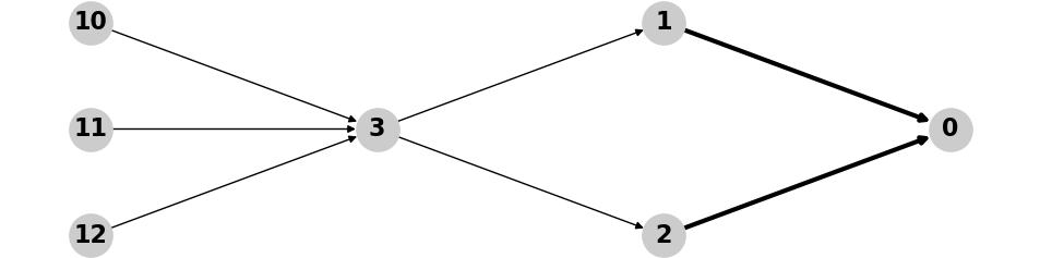
An Active Directory attack graph is denoted by . There are nodes and directed edges. There is one attacker who enters the graph via one of the entry nodes. Let be the total number of entry nodes. We assume that the entry node is selected by nature. For simplicity, we assume uniform chances for all entry nodes. The attacker’s goal is to reach a single destination node called Domain Admin or DA. We consider only one destination.44 4 In real-life Active Directory attack graphs, there are often multiple admin nodes. We simply merge all admin nodes into a single node and call it our DA. There is a set of edges that are blockable, denoted by . Figure 2 is an example graph. The entry nodes are , , and . Node is the destination. The thin edges are blockable (only and are not blockable).
The defender selects the best edges to block, where is the defensive budget. We use to denote the set of edges blocked. We consider only pure actions. That is, we do not study mixed-strategy probabilistic blocking. The graph after blocking is denoted as . We assume the attacker can observe the defensive action and then perform a best-response attack. In the context of Active Directory attack graphs, the attacker performs the shortest path attack on . We use to denote the shortest path from entry node to the destination, on graph .
We assume that an attack path with hops has a success probability of , where could be any decreasing function in . If no attack paths exist, then . can essentially be any performance evaluation function. For presentation purposes, we call it the “success rate”, and we set (i.e., every action has a failure rate).
The defender’s task is to pick the best edges to block, in order to minimize the attacker’s expected success rate. Expectation is taken by averaging over all entry nodes. Formally, our model is the following:
A baseline algorithm is the greedy algorithm (Greedy). We present it here to serve as an example to help readers understand our model. The greedy algorithm will also be used as an algorithm component in later sections.
Algorithm 1 (Greedy).
Given budget , we pick the single best edge to block in terms of reducing the attacker’s expected success rate.55 5 For example, we could use the almost linear algorithm proposed in Nardelli et al. 2001 for each step. We repeat times.
Greedy is actually the optimal algorithm if our graph is exactly a tree. This is straightforward to see. Blocking actions happening in different tree branches are independent from each other. Given edge and , if the path from to DA passes through , then Greedy will always block .
On the other hand, Greedy works poorly if there are substitutable block-worthy edges. For Figure 2, if our budget is , under Greedy, the edges blocked are any two of . Neither nor is blocked. There is still one entry node that can reach DA. The attacker’s success rate is . It is easy to see that the optimal defence should be blocking both and .
4 Hardness and BudgetFPT
We mentioned that Active Directory attack graphs tend to have short attack paths. We first prove that having a small maximum attack path length alone is not enough to derive efficient algorithms.
Theorem 1.
Let be the budget. Let be the maximum attack path length. Our problem is -hard with respect to even for constant .
Theorem 1 implies that having a small maximum attack path length and a small budget is not enough to derive fixed-parameter algorithms, which makes it different from the single source single destination bounded length cut problem studied in Golovach and Thilikos 2011. Nevertheless, the authors’ core idea still applies to our setting. The core idea goes like this: For single source and single destination, we pick an arbitrary shortest path. We must block somewhere along this path. Otherwise, it is as if no blocking happens. Our fixed-parameter algorithm builds on the above idea.
Algorithm 2 (BudgetFPT).
We go over all combinations to find the blocking setup that minimizes the expected success rate for the attacker. We pick an arbitrary entry node and pick an arbitrary shortest path from to DA. We either block at least one edge along this shortest path, or can be removed from our consideration (as its shortest path is unaffected). There are at most options for picking an edge to block. After blocking an edge, the budget is reduced by . There is an option for ignoring . After ignoring , the number of entry nodes is reduced by .
We use to denote the number of combinations we need to go over when the remaining budget is and the remaining number of entry nodes is . We have the following recursive relationship and the base cases:
For each combination, the success rate evaluation takes linear time. We derive the analytical form of , which gives the following complexity result.
Proposition 1.
BudgetFPT has a complexity of
5 Tree Decomposition based Dynamic Program
In this section, we propose a dynamic programming algorithm based on tree decomposition. This algorithm scales the best in experiments, but one restriction is that it requires the attack graph be acyclic. The synthetic attack graph in Figure 1 does contain cycles. However, all cycles involve one common user. So if we remove that one user, the graph becomes acyclic. In other graphs generated using DBCreator, we always only need to remove a few nodes to make the graph acyclic. We argue that the network admin has the flexibility to convert existing graphs into acyclic with minimum changes. Our algorithm can also serve as a heuristic.
The tree width of a graph is a commonly used index to measure how close a graph is to a tree. Many computationally difficult problems on general graphs are easy if the tree width is small. This is also the case for our problem.
Our attack graphs are directed and all nodes have paths to DA (nodes that cannot reach DA are ignored). We further assume that the attack graphs are acyclic in this section. Under the above assumptions, we could use topological sorting to divide our attack graphs into several security levels. DA belongs to the highest security level. An edge only goes from a lower security level node to a strictly higher security level node. Take Figure 2 as an example, we could interpret it as that there are four security levels. to are in the lowest security level while DA (node ) has the highest security level. With this security-level interpretation, there is no ambiguity on the direction of an edge. If an edge involves node and , then the direction must be from to if has a lower security level. We will directly reuse the tree decomposition and tree width definition for undirected graphs.
As an example, Figure 3 shows a tree decomposition of the graph in Figure 2. Every tree node contains a subset of the original graph vertices. The union of all tree nodes contains all graph vertices. Every edge is covered by a tree node. For example, tree node covers all out-going edges of graph vertex . Finally, for every graph vertex, the tree nodes containing it form a subtree. For example, the tree nodes containing are , , and .

Tree decompositions are not unique. The optimal tree decomposition that minimizes the tree width is NP-hard to compute Arnborg et al. 1987. For our dynamic program, we require a specific style of tree decompositions that satisfy extra properties. We call such tree decompositions desired tree decompositions. Figure 3 is a desired tree decomposition. We first explain how we can convert a desired tree decomposition into a dynamic program via an example. During the process, we will explain what it means for a tree decomposition to be desired. Finally, we propose a heuristic that guarantees to generate a desired tree decomposition.
In Figure 3, the number of tree nodes is the same as the number of graph vertices. The first coordinate values are unique. A dynamic program subproblem involves a tree node and a remaining budget . For example, corresponds to the following subproblem: given the remaining budget and the distances (to DA) for and , what should be the distance between and DA? To answer this question, we essentially need to determine the budget investment on (budget spent on is used to block ’s out-going edges). has two successors ( and ). Both successors are blockable, so we could spend to units of budget on . If units of budget is spent on a node (to block its out-going edges), it will always be blocking the shortest paths. Once the budget investment on is determined, ’s final distance is also determined. To summarize, is the subproblem where the defender needs to decide how many units of budget (at most ) are invested on , considering the context information on ’s potential successors (the ). Here, context information refers to the distances to DA.
Let us run through a solution on the basis of Figure 3. Let us recall that the actual graph is in Figure 2. We still assume the total budget is . We start from . The budget investment on will be since its distance to itself is always . This information is then passed down to . has no blockable out-going edges, so we cannot spend any budget anyway. The distance (to DA) for is then . This information is passed down to . Again, we cannot invest any budget because ’s out-going edge is not blockable. We get that ’s distance is . This context is passed down to . At this point, we are deciding how many units of budget to spend on . Based on the context information, we know that and ’s distances are both . The best decision here is to invest units of budget. After that, ’s distance becomes infinity. This information is then passed down to all three leaf nodes. For example, one subproblem at the leaf level is . The context information says that ’s successor ’s distance to DA is infinity, and there is no budget left. So we get ’s distance to DA is also infinity. Since is one of three entry nodes, we add to the expected success rate. Essentially, the original problem is . Our dynamic program makes decisions on the budgets spent on each node. Context information and remaining budgets are passed down to future subproblems. Through out the process, one property we need is that as we move from the root to the leaves, when a vertex first enters into our consideration (i.e., vertex enters at tree node ), the context information (i.e., and ’s distances) must be enough for us to decide the new vertex’ distance right away. That is, for any vertex , we consider the subtree containing . The root of this subtree must contain all out-going edges of . Also, the root of the whole tree should be a node containing DA only. The above properties are not held by all tree decompositions. In this paper, we use the vertex elimination technique to generate tree decomposition Bodlaender et al. 2006. This technique maps an arbitrary permutation of the vertices into a tree decomposition. It should be noted that the vertex elimination technique is only a heuristic framework because it is NP-hard to figure out the best permutation that results in the smallest tree width. Our heuristic is simple: eliminate vertices based on the security level ranking, with the lowest security level eliminated first. We of course cannot guarantee that the generated tree width is the smallest, but it is provable that it generates a tree decomposition that is desired.
Lastly, actually our example in Figure 3 does not capture one complication, which is that at node , we also need to divide the remaining budget among three child branches. We need to divide it four ways (one for itself, for blocking ’s out-going edges; and three for three child branches). This has a complexity of . If there are too many branches, then the decision process gets too expensive. We resolve this using the nice tree decomposition idea from Cygan et al. 2015. The main idea is that we can always clone a node into two. For example, we can insert another in between and . The copy closer to DA only makes the decision on itself (how many units of budget to spend on ). The copy further away from DA deals with the splitting problem for splitting the remaining budget for three children. However, this node still needs to split three ways. The nice tree decomposition idea can resolve this with ease as well. We simply need to add another clone of to handle the second round of splitting. One node splits between and the rest . The second node splits between and . For our setting, the number of clone nodes needed is at most , which does not affect the complexity. The gain is that for every node, the decision is always one dimensional, so the number of decisions at a node is at most .
Proposition 2.
DP has a complexity of
is the achieved tree width using our desired tree decomposition heuristic.
6 Classification-based SplitFPT
Another parameter to describe a graph’s tree-likeness is the number of feedback edges . A related parameter is the number of splitting nodes (nodes with multiple out-going edges). If the maximum out degree is , then we have . For the synthetic graph in Figure 1, the number of splitting nodes is only , and the maximum out degree is only . Having small and essentially means that the attacker’s strategy space is tiny. If the attacker starts from a non-splitting node, then the attacker has no choice but to move on to the only successor, and keeps moving on until 1) the attacker is facing a blocked edge, which means the attacker’s entry node cannot reach DA; 2) the attacker has reached DA; or finally 3) the attacker has reached another splitting node. A path where every intermediate node has only one out-going edge is called a simple path. At a splitting node, an attacker faces at most simple paths (one for each successor). Every simple path leads to either another splitting node or to DA. Essentially, the attacker’s strategy is characterized by his route choices at the splitting nodes. At each splitting node, there are at most options, including at most simple paths to choose from, and not choosing at all, which happens if none of the simple paths leads to DA. The attacker’s strategy space has a size of .
Typically for Stackelberg games, we optimize over the defender’s strategy space. For each defender’s strategy, we figure out the attacker’s best-response, and then check how good this best-response attack is in terms of the defender’s utility. In this paper, because the attacker’s strategy space is tiny, we instead optimize over the attacker’s strategy space. We guess what the attacker would do when facing the optimal defence. That is, we guess the attacker’s route choices at the splitting nodes. When both and are tiny, we can simply go over all strategies of the attacker. If we go over all combinations, then at least one is indeed the best response to the optimal defence. Given a guessed attacker’s strategy, we can derive the distances (to DA) from all splitting nodes. For example, given split node , we know what route the attacker would choose at this node, which has to be the shortest unblocked route, since we assume it is a best response. We can follow along this simple path to another splitting node (or to DA). At the next splitting node, we also know what route the attacker would choose. This way we can generate the shortest paths from all splitting nodes to DA, except for splitting nodes at which the attacker chooses not to take any route (the distances are set to infinity for these nodes). For all generated shortest paths, we mark all blockable edges covered by them as not blockable. The defender cannot block these edges, otherwise it is contradictory to our assumption that the attacker’s strategy is a best response. Then, at each splitting node, there are routes not taken by the attacker (either all but one are not taken, or simply all are not taken). Let us consider a splitting node , and one of its successors , where route is not taken. We follow the simple path starts from , and continue on until we either reach DA or another splitting node. We always end up with a node whose distance to DA is known. We calculate whether the simple path under discussion is a better choice for the attacker or not. If not, we do not need to do anything. If it is a better choice for the attacker, then we must block this simple path. Again, otherwise it is contradictory to our assumption that the attacker’s strategy is the best response to the optimal defence. For a simple path, it is without loss of generality to block the blockable edge that is closest to DA. There is no reason to block further away edges or multiple edges. After the above actions (marking some edges as not blockable and blocking some edges), we end up with an attack graph that is exactly a tree (only one rational decision at any splitting node). When the attack graph is a tree, we simply run Greedy using the remaining budget.
Proposition 3.
SplitFPT has a complexity of
7 Graph Convolutional Neural Networks
SplitFPT exhaustively goes over the attacker’s options at all splitting nodes. This is exactly a node classification problem. We use graph convolutional neural network to perform node classification so that it scales to larger graphs.
We perform unsupervised learning as follows. A node classification neural network takes one splitting node as input, and outputs its classification (i.e., which route the attacker would take when facing the optimal defence; the attacker may take no routes, which is just another classification category). Given a classification on the splitting nodes, we can evaluate the corresponding defence that would induce this classification using the same procedure in SplitFPT. That is, we can map a node classification to an expected success rate for the attacker.
A short description of our neural network approach is that, given the current neural network (the current node classification rule), we randomly flip some nodes’ classifications to check whether the perturbed classification leads to better result (worse success rate for the attacker). If so, we instruct the neural network to learn toward the better classification (treat it as true labels). We obviously do not have the computational resources to exhaustively go over all node classification combinations (otherwise we should simply run SplitFPT). The goal is to get a small number of nodes’ classifications correct, and hope the neural network is able to pick up the underlying rules, and can help generalize to produce correct classifications on all nodes.
Below are the details of our neural network.
Node and edge features: Because the original graph is too large to handle, we construct a condensed graph containing only the splitting nodes. The splitting nodes are connected via simple paths in the original graph. In the condensed graph, a simple path is interpreted as a single edge. An example node feature is its out degree. An example edge feature is the length of the corresponding simple path. Due to space constraint, we omit our list of manually derived features ( node features, edge features).
Network structure: Both the node features and the edge features are expanded to dimensions using linear encoders. The features then go through layers of crystal graph convolutional layer with max as the aggregator and batch normalization turned on Xie and Grossman 2018. Between each layer, we have a dropout layer that drops an edge with probability. The last layer is a linear layer that converts the output to dimensions. Given an output, the coordinate with the highest value is taken as the neural network’s classification for the input splitting node.
Training: We use a batch size of (splitting nodes). For splitting nodes not in the batch, their classifications follow the current network’s decision. For a node in the batch, with probability, we follow the current network’s classification, but we do not just pick the coordinate with the highest value. Instead, we use softmax to get each dimension’s probability and we draw a classification accordingly. With probability, we disregard the network and draw a classification uniformly at random. Essentially, we slightly perturb the in-batch nodes’ classifications. We then go over the in-batch nodes one by one based on a random permutation order. For each node, we exhaustively go over all classifications and check whether unilateral change leads to a better-performing classification. We end up with a new classification. With probability, we use this new classification as true labels. With the other chance, we use the historically best-performing classification as true labels. We stop after epochs. Loss is based on cross entropy and the optimizer is Adam with a learning rate of . We also always train times with random seed to .
8 Experiments
Our hardware specs are i7-6700 3.4GHz and double TURBO-GTX1080-8G GPUs. We conduct all experiments using a synthetic Active Directory attack graph generated by DBCreator. We set the number of computers to . We only consider three types of edges: AdminTo, MemberOf, HasSession. These three edge types are the only three default edge types in BloodHound. The final graph contains nodes (computers + user accounts + security groups, etc.) and edges.66 6 There are admin nodes. We merge them into one node DA. Out of nodes, only can reach DA. So we can preprocess our graphs to make it much smaller. We call this graph r2000. We can make r2000 acyclic by removing another nodes from it. We call the acyclic version r2000-dag.
We randomly set some edges to be blockable. For a non-splitting node, its out-going edge is blockable with probability. For a splitting node, with probability, all of its out-going edges are blockable. We set to be . All of our experiments are repeated times.
Table 1: Low budget setting. We randomly pick nodes to be the entry nodes. We set the budget to . With a small budget and a small number of entry nodes, BudgetFPT is scalable. We compare BudgetFPT against Greedy and GCN (the graph convolutional neural network approach). Note that BudgetFPT is optimal. Success Rate is short for the expected success rate for the attacker (lower is better). Time[s] is seconds per trial. #Opt shows how many times the algorithm under discussion produces a result that is within of the optimal result (among trials).
| Success Rate | Time[s] | #Opt | |
|---|---|---|---|
| BudgetFPT | |||
| GCN | |||
| Greedy |
Table 2: Acyclic setting. We use r2000-dag instead. We compare DP against Greedy and GCN. It turns out that both GCN and Greedy always achieve the optimal results. Greedy being optimal is not entirely surprising, because we have shown that Greedy is optimal if the graph is exactly a tree, and r2000-dag is very close to a tree.
| Success Rate | Time[s] | #Opt | |
|---|---|---|---|
| DP | |||
| GCN | |||
| Greedy |
Table 3: Acyclic setting with substitutable edges. We could artificially modify r2000-dag and create an acyclic graph that is not close to a tree. We recall that Greedy fails when there are substitutable blockable-worthy edges, as shown in Figure 2. We introduce substitutable edges into r2000-dag. Given a blockable edge , we duplicate . We create two paths and , where is a successor of . Essentially, we are recreating the structure of Figure 2. This setup is actually simulating a practical scenario. If there are two different exploits that allow the attacker to travel from to , then we need to block both exploits. Under this artificially created acyclic graph, GCN is still always getting the optimal result, and Greedy fails out of trials.
| Success Rate | Time[s] | #Opt | |
|---|---|---|---|
| DP | |||
| GCN | |||
| Greedy |
Table 4: Setting without optimal solutions. We go back to r2000. We double the budget to and double the number of entry nodes to . We can no longer afford to run BudgetFPT. We also cannot run DP because r2000 contains cycles. In this setting, we do not have optimal solutions. We compare Greedy against GCN. #Win refers to how many times an algorithm beats the other one (ties are not counted as wins). It turns out that Greedy performs better than GCN in this setting. In r2000, there are naturally occurring substitutable edges. With double budget, Greedy will block the substitutable edges despite they are perceived as low in priority (i.e. no place to spend the budget, so might as well spend on substitutable edges). If we double , then Greedy again has plenty of places to spend budget on, so it will not spend budget on substitutable edges. As a result, GCN constantly wins again.
| Success Rate | Time[s] | #Win | |
| GCN () | |||
| Greedy () | |||
| GCN () | |||
| Greedy () |
9 Conclusion
We studied edge blocking for defending Active Directory style attack graphs. We proposed fixed-parameter algorithms based on the observation that practical Active Directory attack graphs have small maximum attack path lengths and are similar to trees. BudgetFPT can be applied when both the budget and the number of entry nodes are small. DP scales the best experimentally, but it is only applicable to acyclic graphs. SplitFPT is based on performing fixed-parameter analysis on the attacker’s strategy space, which happens to be much smaller compared to the defensive strategy space in our model. For each attacking strategy, we analysed what kind of defense would make this attacking strategy a valid best response. This FPT technique is potentially useful for other Stackelberg games. Lastly, we scaled up SplitFPT by converting it to a graph convolutional neural network based heuristic. A typical FPT approach is to exhaustively search among a set of solutions characterized by the fixed parameters. Instead of exhaustive search, we trained a neural network to guess the best solution. Our algorithms will help IT admins to identify high-risk edges (accesses/exploits) in practical Active Directory environments.
Acknowledgements
Frank Neumann has been supported by the Australian Research Council through grant FT200100536. Hung Nguyen is partially supported by the “Cyber NGT – Provable Network Security” grant.
References
- Lallie et al. [2020] Harjinder Singh Lallie, Kurt Debattista, and Jay Bal. A review of attack graph and attack tree visual syntax in cyber security. Computer Science Review, 35:100219, February 2020. ISSN 15740137. doi:10.1016/j.cosrev.2019.100219.
- Dunagan et al. [2009] John Dunagan, Alice X. Zheng, and Daniel R. Simon. Heat-ray: Combating identity snowball attacks using machinelearning, combinatorial optimization and attack graphs. In Proceedings of the ACM SIGOPS 22nd Symposium on Operating Systems Principles - SOSP ’09, page 305, Big Sky, Montana, USA, 2009. ACM Press. ISBN 978-1-60558-752-3. doi:10.1145/1629575.1629605.
- Paruchuri et al. [2008] Praveen Paruchuri, Jonathan P. Pearce, Janusz Marecki, Milind Tambe, Fernando Ordonez, and Sarit Kraus. Efficient algorithms to solve Bayesian Stackelberg games for security applications. In Proceedings of the 23rd National Conference on Artificial Intelligence - Volume 3, AAAI’08, pages 1559–1562, Chicago, Illinois, July 2008. AAAI Press. ISBN 978-1-57735-368-3.
- Bar-noy et al. [1995] Amotz Bar-noy, Samir Khuller, and Baruch Schieber. The Complexity of Finding Most Vital Arcs and Nodes. Technical report, University of Maryland, 1995.
- Chen et al. [2006] Jianer Chen, Iyad A. Kanj, and Ge Xia. Improved Parameterized Upper Bounds for Vertex Cover. In Rastislav Královič and Paweł Urzyczyn, editors, Mathematical Foundations of Computer Science 2006, Lecture Notes in Computer Science, pages 238–249, Berlin, Heidelberg, 2006. Springer. ISBN 978-3-540-37793-1. doi:10.1007/11821069_21.
- Milgram [1967] Stanley Milgram. The Small-World Problem. Psychology Today, 1:61–67, 1967.
- Arnborg et al. [1987] Stefan Arnborg, Derek G. Corneil, and Andrzej Proskurowski. Complexity of finding embeddings in a k-tree. Siam Journal of Discrete Mathematics, 8(2):277–284, 1987.
- Bazgan et al. [2019] Cristina Bazgan, Till Fluschnik, André Nichterlein, Rolf Niedermeier, and Maximilian Stahlberg. A more fine-grained complexity analysis of finding the most vital edges for undirected shortest paths. Networks, 73(1):23–37, 2019. ISSN 1097-0037. doi:10.1002/net.21832.
- Golovach and Thilikos [2011] Petr A. Golovach and Dimitrios M. Thilikos. Paths of bounded length and their cuts: Parameterized complexity and algorithms. Discrete Optimization, 8(1):72–86, February 2011. ISSN 15725286. doi:10.1016/j.disopt.2010.09.009.
- Dvořák and Knop [2018] Pavel Dvořák and Dušan Knop. Parameterized Complexity of Length-bounded Cuts and Multicuts. Algorithmica, 80(12):3597–3617, December 2018. ISSN 1432-0541. doi:10.1007/s00453-018-0408-7.
- Aziz et al. [2018] Haris Aziz, Serge Gaspers, Edward J. Lee, and Kamran Najeebullah. Defender Stackelberg Game with Inverse Geodesic Length as Utility Metric. In Proceedings of the 17th International Conference on Autonomous Agents and MultiAgent Systems, AAMAS ’18, pages 694–702, Richland, SC, July 2018. International Foundation for Autonomous Agents and Multiagent Systems.
- Aziz et al. [2017] Haris Aziz, Serge Gaspers, and Kamran Najeebullah. Weakening Covert Networks by Minimizing Inverse Geodesic Length. In Proceedings of the Twenty-Sixth International Joint Conference on Artificial Intelligence, pages 779–785, Melbourne, Australia, August 2017. International Joint Conferences on Artificial Intelligence Organization. ISBN 978-0-9992411-0-3. doi:10.24963/ijcai.2017/108.
- Durkota et al. [2019] Karel Durkota, Viliam Lisý, Branislav Bošanský, Christopher Kiekintveld, and Michal Pěchouček. Hardening networks against strategic attackers using attack graph games. Computers & Security, 87:101578, November 2019. ISSN 01674048. doi:10.1016/j.cose.2019.101578.
- Milani et al. [2020] Stephanie Milani, Weiran Shen, Kevin S. Chan, Sridhar Venkatesan, Nandi O. Leslie, Charles Kamhoua, and Fei Fang. Harnessing the Power of Deception in Attack Graph-Based Security Games. In Quanyan Zhu, John S. Baras, Radha Poovendran, and Juntao Chen, editors, Decision and Game Theory for Security, Lecture Notes in Computer Science, pages 147–167, Cham, 2020. Springer International Publishing. ISBN 978-3-030-64793-3. doi:10.1007/978-3-030-64793-3_8.
- Wang et al. [2019] Kai Wang, Aditya Mate, Bryan Wilder, Andrew Perrault, and Milind Tambe. Using Graph Convolutional Networks to Learn Interdiction Games. In AI for Social Good Workshop, International Joint Conference on Artificial Intelligence (IJCAI), 2019.
- Dai et al. [2017] Hanjun Dai, Elias B. Khalil, Yuyu Zhang, Bistra Dilkina, and Le Song. Learning combinatorial optimization algorithms over graphs. In Proceedings of the 31st International Conference on Neural Information Processing Systems, NIPS’17, pages 6351–6361, Red Hook, NY, USA, December 2017. Curran Associates Inc. ISBN 978-1-5108-6096-4.
- Nardelli et al. [2001] Enrico Nardelli, Guido Proietti, and Peter Widmayer. A faster computation of the most vital edge of a shortest path. Information Processing Letters, 79(2):81–85, June 2001. ISSN 00200190. doi:10.1016/S0020-0190(00)00175-7.
- Bodlaender et al. [2006] Hans L. Bodlaender, Fedor V. Fomin, Arie M. C. A. Koster, Dieter Kratsch, and Dimitrios M. Thilikos. On Exact Algorithms for Treewidth. In Yossi Azar and Thomas Erlebach, editors, Algorithms – ESA 2006, Lecture Notes in Computer Science, pages 672–683, Berlin, Heidelberg, 2006. Springer. ISBN 978-3-540-38876-0. doi:10.1007/11841036_60.
- Cygan et al. [2015] Marek Cygan, Fedor V. Fomin, Łukasz Kowalik, Daniel Lokshtanov, Daniel Marx, Marcin Pilipczuk, Michał Pilipczuk, and Saket Saurabh. Parameterized Algorithms. Springer International Publishing, 2015. ISBN 978-3-319-21274-6. doi:10.1007/978-3-319-21275-3.
- Xie and Grossman [2018] Tian Xie and Jeffrey C. Grossman. Crystal Graph Convolutional Neural Networks for an Accurate and Interpretable Prediction of Material Properties. Physical Review Letters, 120(14):145301, April 2018. doi:10.1103/PhysRevLett.120.145301.
- Fellows et al. [2009] Michael R. Fellows, Danny Hermelin, Frances Rosamond, and Stéphane Vialette. On the parameterized complexity of multiple-interval graph problems. Theoretical Computer Science, 410(1):53–61, January 2009. ISSN 0304-3975. doi:10.1016/j.tcs.2008.09.065.
Appendix
9.1 Proof of Theorem 1
Proof.
We reduce clique to our problem. Clique is known to be -hard with respect to the clique size Fellows et al. 2009. Let be an arbitrary clique instance. is an undirected graph. For each edge from , we construct one corresponding entry node in attack graph . For every node from , we construct two nodes and in attack graph . We assume connects node and node from . We create two paths and . That is, ’s shortest path to DA has length unless both and are blocked. The best way to spend a defensive budget of is to locate a clique of size in . Only by locating a clique, the defender can disconnect a maximum of entry nodes.
We then calculate the size of the constructed attack graph . If has nodes and edges, then the attack graph has nodes (one node for each edge in , two nodes for each node in , and finally DA) and edges (two edges from each and for each node in , one edge for connecting and and one edge for connecting to DA). If a fixed-parameter tractable algorithm exists with respect to for the attack graph , then its complexity must be , which is then . But then this means it is fixed-parameter tractable to find a clique of size in the Clique instance , which is contradictory to Clique being -hard. ∎
BudgetFPT(, )
Input: Attack graph , budget
Output: Attacker’s expected success rate
9.2 Proof of Proposition 1
Proof.
We have the following recursive relationship and the base cases:
We define the as follows
As a result, we have the following much more elegant recurrence relationship:
We use the standard generating function trick to analyse the recurrence relationship for . We define as follows
Since , we have
is from the term . The coefficient for is . Therefore, we have
Above we have calculated the number of combinations. For each combination, performance evaluation takes linear time, so the overall complexity is
It should be noted that according to the pseudocode, we need to calculate shortest path (linear time) over and over again to generate all combinations. When budget is , we calculate one shortest path (linear time) and this cost is distributed on combinations. When budget equals , we calculate one shortest path and this cost is distributed on combinations. For each combination, the cost distributed on it for computing shortest path is linear time, multiplied by . Therefore, for each combination, the computation time is still linear. ∎
9.3 Pseudocode for Dynamic Program
Step 1: generate a desired tree decomposition
Desired tree decomposition heuristic
Step 2: generate auxiliary tree nodes according to the nice tree decomposition idea (Cygan 2015)
Add auxiliary tree nodes
Step 3: dynamic program subproblems
- •
Subproblem on non-auxiliary node and remaining budget : The task is to optimally allocate budget on this node (remaining budget is passed down to current node’s only predecessor, which must be an auxiliary node), in order to minimize the expected success rate of the attacker assuming that the attacker starts from an entry node that belongs to the current subtree. The context information is the s’ distances to DA. We decide how many units of budget to spend on itself to block its out-going edges to the . If ’s distance to DA is , then unless the edge is blocked (or it does not exist), has a path of length to DA. If units is spent on , then we will always be blocking the shortest options.77 7 We need to sort options. We treat this as in complexity analysis, because our algorithm can only realistically handle single digit tree width . Alternatively, we could multiply to the complexity result. We go through options (spend to ) to find the optimal unit of budget to spend on itself. Once ’s distance is decided, the distance is passed down as part of the context information to the only predecessor node, which must be an auxiliary node. The remaining budget is also passed down. The result of the current subproblem is equal to the result of the predecessor’s subproblem. If is an entry node, we also need to add to the result of the current subproblem.
- •
Subproblem on auxiliary node and remaining budget : The task is to optimally split the remaining budget to its predecessor nodes, in order to minimize the expected success rate of the attacker assuming that the attacker starts from an entry node that belongs to the current subtree. There are at most two predecessors. We need to divide between the two predecessors. That is, pass to one predecessor and to the other predecessor. Sum up the two return values from the two predecessors’ subproblems. The splitting scheme corresponding to the minimum sum is the chosen scheme.
SplitFPT
Greedy on exact trees (subroutine of SplitFPT)
Input: Remaining budget
9.4 Proof of Proposition 2
Proof.
There are nodes. For each node, there are coordinates for tracking distances. Each coordinate has options ( to , and infinity). Every subproblem also tracks the remaining budget. The number of subproblems is . Finally, each subproblem is an aggregation of at most subproblems. ∎
9.5 Proof of Proposition 3
Proof.
The number of strategy combinations for the attacker is , where is the number of splitting nodes and is the out degree of splitting node . This value is at most , because if there are feedback edges, spreading them on different splitting nodes (out degree ) would maximize the number of combinations for the attacker’s strategies.
Given a specific attacker strategy, we have to mark all taken simple paths as unblockable. There are at most simple paths. The length is at most each. So this step takes . We also need to construct a spanning tree for the splitting nodes in order to calculate these nodes’ distances to DA under the current attacking strategy. We could implement a small graph with splitting nodes only, and the edges are weighted (based on the lengths of the corresponding simple paths). The number of splitting nodes is at most . Assuming a simple adjacency matrix implementation, this step takes . We then need to check and block all simple paths not taken. This steps takes . Finally, we need to run Greedy to spend the remaining budgets. Greedy takes linear time to locate one edge to block when the attack graph is a tree. It is repeated times at most. So this step takes . ∎
9.6 Node features used in graph convolutional neural networks
- •
A node’s security level (based on topological sorting)
- •
In degree
- •
Out degree
- •
Number of entry nodes that can reach this node
- •
Distance to DA assuming no edges are blocked
- •
Distance to DA assuming all edges are blocked
- •
Whether this node is an entry node
9.7 Edge features used in graph convolutional neural networks
Every edge in the condensed graph corresponds to a simple path from the original graph.
- •
First node of the simple path
- •
Length of the simple path
- •
How many edges can be blocked along the simple path
- •
Security level of the destination node from the blockable edge that is closest to DA
- •
How many entry nodes are along the simple path
- •
Direction (incoming or out-going)