Integrating Quantum Processor Device and Control Optimization
in a Gradient-based Framework
Abstract
In a quantum processor, the device design and external controls together contribute to the quality of the target quantum operations. As we continuously seek better alternative qubit platforms, we explore the increasingly large device and control design space. Thus, optimization becomes more and more challenging. In this work, we demonstrate that the figure of merit reflecting a design goal can be made differentiable with respect to the device and control parameters. In addition, we can compute the gradient of the design objective efficiently in a similar manner to the back-propagation algorithm Rumelhart et al. 1986 and then utilize the gradient to optimize the device and the control parameters jointly and efficiently. This extends the scope of the quantum optimal control to superconducting device design. We also demonstrate the viability of gradient-based joint optimization over the device and control parameters through a few examples.
Quantum mechanics provides an entirely new way to think about information processing. Information is stored in quantum systems and the dynamics are described by the Schrödinger equation or the master equation. To achieve desired operations, we need to design systems with suitable Hamiltonians and dissipation as well as time-dependent external controls. Concrete examples of such quantum information processing tasks include quantum computing, quantum simulation, quantum error correction, and quantum metrology. At this level of abstraction, it is clear that we are dealing with optimization problems that consist of both Hamiltonian design and control. Traditionally, the optimization of the design Menke et al. 2021; Liu et al. 2021 and the optimization of the control Khaneja et al. 2005; Machnes et al. 2018 are usually studied separately. In this work, we treat them as equal components in a single optimization problem and use gradient information to speed up optimization.
We consider superconducting circuits, which are one of the most promising hardware platforms due to their device design versatility and fabrication scalability. While the design versatility allows for many qubit and coupling types Yamamoto et al. 2003; Chiorescu et al. 2003; Izmalkov et al. 2004; Plourde et al. 2004; Koch et al. 2007; Majer et al. 2007; Barends et al. 2014; Manucharyan et al. 2009; Yan et al. 2018; Ofek et al. 2016, it also makes the quest of finding the best design harder due to the larger parameter space. As mentioned earlier, the optimization of the device design is further complicated by the fact that we need to consider the control schemes simultaneously, which has been noted in previous work Chu and Yan 2021; Goerz et al. 2017. For example, complex control schemes are needed for bosonic code qubits, and often numerical optimization is required to obtain the best gate performances Heeres et al. 2017; Hu et al. 2019; Wang et al. 2021. In scenarios where we cannot estimate the control performances with analytical formulas, the optimization problem of the qubit design inevitably becomes a joint optimization problem of design and control with an even larger parameter space. A common strategy to handle large optimization problems is using efficiently computed gradients to help us traverse the optimization landscape. One milestone in this direction is the GRadient Ascent Pulse Engineering (GRAPE) algorithm Khaneja et al. 2005. In this work, we showed that the figure of merit of a target goal such as the gate fidelity can be made differentiable with respect to the parameters from the device and the control together. The gradients can be computed in a single computation similar to the GRAPE algorithm and the back-propagation algorithm Rumelhart et al. 1986. More accurately, the ratio of the time needed to compute the figure of merit and its gradient is independent of the number of control parameters. This makes our method feasible not only for optimizing complex pulse shapes but also for optimizing large processor device designs, and more interestingly, jointly optimizing the design and control.

Integrating design and control aspects. In this work, we mainly focus on the two stages of quantum processor design that involve finding optimal values of the device parameters in the system Hamiltonian and deriving optimal control pulses to maximize the performance of the target quantum processor. When the device parameters are determined and we only need to optimize over the control parameters for better performance or robustness, this is precisely what quantum optimal control and robust control do. In contrast, we may sometimes need to optimize the spectral or other properties of the device Hamiltonian itself, e.g., for determining tunable -interaction on–off ratios DiCarlo et al. 2009; Stehlik et al. 2021 or for designing 4-local interaction couplers Menke et al. 2021.
Now we introduce our framework that unifies the above two scenarios, optimizing a system’s performance over the control parameters and the device parameters jointly as illustrated in Fig. 1. The Hamiltonian of a quantum system with control fields takes the following form:
| (1) |
where , , and are the device Hamiltonian, control operators, and control fields, respectively, and and denote the device and control parameters, respectively. The goal is to optimize and for certain objectives, such as implementing a specific unitary operator within a given time . This extended setup formulates a device-control codesign problem. In Appendix A, we explain why we expect that optimizing and simultaneously will be more efficient compared to the case where we artificially break the optimization problem into two and optimize and alternatively. Compared to the optimal control problem where is fixed, the extended setup will open more possibilities. For example, we can optimize the device parameters for a gate implementation that is robust against control fluctuations and deviations. We will later showcase this by using our method to obtain a more robust iSWAP gate between capacitively coupled fluxonium qubits. In comparison, with conventional quantum control, we only optimize over control parameters for robust schemes.
Efficient gradient computation for both device and control parameters. Here, we discuss an efficient method for computing the gradient of both the device and control parameters. More explanation about why we consider this method to be efficient can be found in Appendix B. For a superconducting processor using qubits as its basic components, the total Hilbert space can be decomposed correspondingly as , where each is typically an infinite-dimensional Hilbert space. The time-independent Hamiltonian in Eqn. 1 can be typically described by the Hamiltonian
| (2) |
where and are single component Hamiltonian and coupling operators defined on , respectively. The concrete form of depends on the type of coupling between qubits. For notational simplicity, we assume that there is a single type of coupling, but our computation method naturally generalizes to the situation where there are multiple types. We will also assume that there is a single control operator (see Eqn. 1) for each subsystem .
Even though each component has infinite dimensions, typically only the lowest few energy eigenstates will participate in the computation. This is indeed the case for the examples presented in this work. Therefore, an efficient method for performing numerical simulations is to first truncate the total Hilbert space into this relevant subspace , where is the low energy subspace under the above assumption. This can be done by diagonalizing . We can then use the operators from projecting , , and into the subspace as an approximation and obtain an efficient finite dimensional Hamiltonian for numerical computation. Both the Hamiltonian diagonalization and the Hilbert space truncation can be made differentiable. Please refer to Appendix B for technical details. To the best of our knowledge, this is the first attempt to extend the GRAPE algorithm Khaneja et al. 2005 to superconducting circuit device parameters.
The evolved unitary operator at time can be then derived by solving the ordinary differential equation (ODE)
| (3) |
After we compute , we can use objective functions such as the average gate fidelity Nielsen and Chuang 2000 to compute how close and the desired operator are. In general, we need to add more terms to the objective functions to ensure the devices are practical. For now, we assume that it is easy to perform the reverse-mode differentiation for the computation steps to compute the objective function from . To make the whole design workflow differentiable, we still need to perform reverse-mode differentiation through the ODE solver. The adjoint sensitivity method Pontryagin et al. 1962 makes this possible. This method computes gradients by solving a second, augmented ODE backwards in time, independent of the parameter size. With the gradients computed in reverse mode, we can now optimize over the device and control parameters jointly and efficiently for an objective .
The proposed framework may also be used to optimize for solutions robustly against control noise. Robust optimization over control parameters has been extensively studied Zhang et al. 2014; Chen et al. 2014; Kabytayev et al. 2014. Here, we take a sample-based approach Zhang et al. 2014; Chen et al. 2014 and define
| (4) |
where is the original design goal, e.g., the fidelity or another figure of merit, is the number of samples, and is the deviation of caused by noise in the -th sample. Optimizing will make parameters robust against the selected noise. Since we can compute the gradient of , we can compute the gradient of by summing over the gradients of . In this way, we can also use the gradient information to speed up the robustness optimization.
As mentioned above, there are scenarios where we want to optimize the properties of alone. In Appendix F, we will show how we can choose an objective function for a large -interaction on–off ratio between two transmon qubits and the gradient computation method.
iSWAP gate with fluxonium qubits We will demonstrate our method for an iSWAP between two capacitively coupled fluxonium qubits, the diagram of which is depicted in Fig. 2(a).
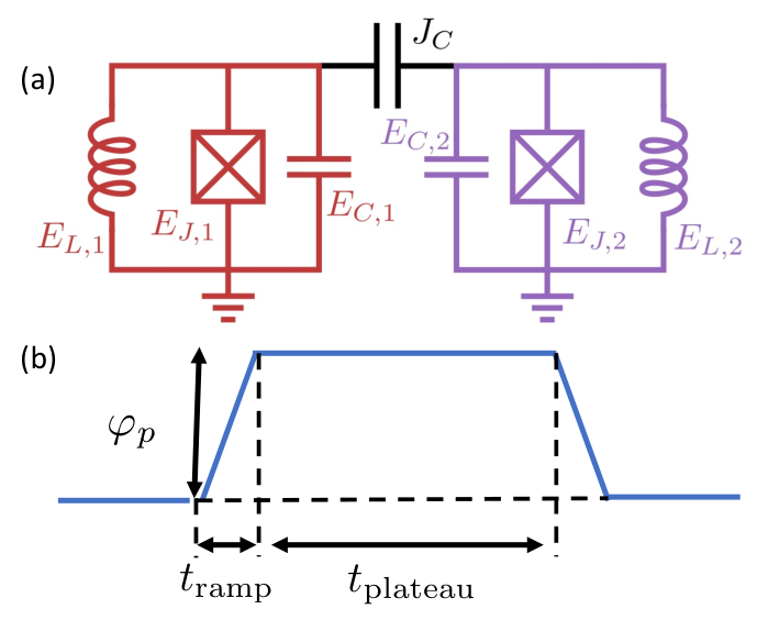
The Hamiltonian of the system is
| (5) |
where is the coupling strength between the two qubits, and is the Hamiltonian of the -th fluxonium qubit Manucharyan et al. 2009, defined as follows:
| (6) |
where , , and are the charging energy, the Josephson energy, and the inductive energy, respectively, is the phase operator, and is the conjugate charge operator. We set the external flux of the second qubit to be a time-dependent control field initially at , while for the first qubit, the external flux is fixed to be , that is, and . The waveform of is chosen to be a trapezoid pulse as shown in Fig. 2(b), which is given by
| (7) |
where and are the external flux bias and holding time of the plateau of the waveform, is the time for the rising and falling edges, and is a commonly used activation function in neural networks. We call , , , and the device parameters, and the parameters in are the control parameters 11 1 Though was part of the device Hamiltonian, it comes from the external flux control, so the parameters therein are more appropriately regarded as control parameters.. These are all parameters involved in the optimization.
Some details of the construction of the finite dimensional Hamiltonian are provided in what follows. We first write the Hamiltonian of the single-qubit fluxonium in the discretized phase basis over a finite range of phase values. To obtain sufficiently accurate low-energy eigenstates for the optimization task, we select the range to be and the number of basis points to be .
We select the average fidelity to be the objective function. The leakage is small for the iSWAP gate scheme, and the optimized results have a leakage smaller than . Therefore, it is a good approximation to compute the fidelity based on the truncated unitary matrix. However, there are usually single qubit phases accumulated during the implementation of the gate, and we can compensate for these phases at a very low cost McKay et al. 2017. Therefore, we will use a modified average fidelity with phase compensation included (see Appendix D). We include other terms in the total objective function. One is a penalty , which roughly estimates the infidelity caused by the decoherence of and . Another is , which discourages the frequencies of the two fluxonium qubits from being too close. This is useful for having addressable single qubit gates and it mitigates -crosstalk when both fluxonium qubits are at their sweet spots. The last one is , which forces the fluxonium parameters to be realistic for fabrication. The exact forms of these terms will be given in Appendix E.
In total, we set the objective function for minimization to be
| (8) |
Another desired feature of the iSWAP gate scheme is robustness against control errors. Here, we demonstrate how we can improve the robustness of the gate fidelity with respect to the amplitude parameter in Eqn. 7. To do this, we set , i.e., all the control parameters in other than are set to . Then, we can construct the robustness objective function from according to Eqn. 4. We use the Adam optimizer Kingma and Ba 2015 to minimize the objective functions and . For the initial condition and optimizer hyperparameters listed in Appendix E, the objective functions during optimization are shown in Fig. 3, and the comparison of the result’s robustness is shown in Fig. 4. While the optimization of has not converged, the result is good enough for the current experimental capabilities and demonstrating the viability of gradient optimization. As shown in Fig. 4, the parameters obtained by optimizing are indeed more robust with respect to the errors in compared to obtained by optimizing , and the minimum is lower. The latter effect was unintended. Retrospectively, due to the change of the objective function, escaped the local minimum of .
With this example, we show that the joint gradient optimization is viable for a practical problem. Because both capcitively coupled fluxonium qubits and the control pulse Eqn. 7 have been realized in the experiment Bao et al. 2021 and their behaviours coincide with the numerical simulation, we expect the gain from doing the optimization can transfer to the experiments as long as we have the correct decoherence model. For the optimization of objective , we reach a local minimum of both the device and control parameters in a single run of the gradient optimization. To understand the benefits of using reverse-mode gradient computations in the optimization, we can compare the speed of the reverse-mode gradient computation with the computation of finite differences (see Appendix B for an explanation of finite differences). This is because finite differences are widely used to estimate the gradients in the implementation of popular optimizers. For example, this is how the Broyden–Fletcher–Goldfarb–Shanno (BFGS) algorithm Nocedal and Wright 2006; Byrd et al. 1995 in SciPy Virtanen et al. 2020 estimates the gradients when they are not provided by the user. The speedup is about three times for this small optimization problem with seven device parameters and three control parameters (see Appendix E for the running time). In Appendix C, we use the task of diagonalizing fluxonium Hamiltonians to demonstrate that the speedup of the gradient optimization will grow when the system size and the number of parameters grow.
Discussion In this work, we extend the optimal control framework to superconducting circuit parameters. We showcase that we can optimize over the device and control parameters jointly for a figure of merit reflecting a design goal through reverse-mode gradient computation. This suggests that there is almost no downside in terms of the efficiency to add device parameters to the optimization variables.
We can further extend the proposed framework to other stages of quantum processor design. The Hamiltonian representation with device parameters such as , , and we discussed in the paper is an intermediate representation when designing a quantum processor. This representation is derived from the underlying lumped-element circuit representation, which is again derived from the processor’s two-dimensional (2D)/three-dimensional (3D) layout representation. There could be more freedom or design choices in the lumped-element circuit or layout representations. Moreover, the layout representation allows us to estimate substantial losses, such as the dielectric loss, based on the electric field energy distribution on the interfaces with contamination. However, electromagnetic simulations, which are used to evaluate the layout design, are very computationally expensive. This means that the gradient evaluation of the Hamiltonian parameters with respect to the layout parameters may be of substantial importance, as they will significantly reduce the number of iterations. We leave this for future study.
Most optimal control use cases focus on optimizing control solutions to realize a given quantum operation. However, for NISQ (noisy intermediate-scale quantum) applications or quantum error correction, the overall performance depends on native gates available on the device, the compilation scheme used, and other device aspects like the readout and reset.
In Appendix F, we illustrate how we can simultaneously optimize the -interaction on–off ratios on different pairs of transmon qubits on a square lattice amenable to fault-tolerant quantum error correction architectures such as the surface code. This can be viewed as a first step toward task-oriented optimization.
The authors would like to thank Dawei Ding and Fei Yan for their constructive comments and Yaoyun Shi for his encouragement and proof-reading of the manuscript.
References
- Rumelhart et al. (1986) D. E. Rumelhart, G. E. Hinton, and R. J. Williams, Nature 323, 533 (1986).
- Menke et al. (2021) T. Menke, F. Häse, S. Gustavsson, A. J. Kerman, W. D. Oliver, and A. Aspuru-Guzik, npj Quantum Information 7, 1 (2021).
- Liu et al. (2021) F.-M. Liu, M.-C. Chen, C. Wang, S.-W. Li, Z.-X. Shang, C. Ying, J.-W. Wang, C.-Z. Peng, X. Zhu, C.-Y. Lu, et al., arXiv preprint arXiv:2109.00994 (2021).
- Khaneja et al. (2005) N. Khaneja, T. Reiss, C. Kehlet, T. Schulte-Herbrüggen, and S. J. Glaser, Journal of Magnetic Resonance 172, 296 (2005).
- Machnes et al. (2018) S. Machnes, E. Assémat, D. Tannor, and F. K. Wilhelm, Physical review letters 120, 150401 (2018).
- Yamamoto et al. (2003) T. Yamamoto, Y. A. Pashkin, O. Astafiev, Y. Nakamura, and J. S. Tsai, Nature 425, 941 (2003).
- Chiorescu et al. (2003) I. Chiorescu, Y. Nakamura, C. J. P. M. Harmans, and J. E. Mooij, Science 299, 1869 (2003).
- Izmalkov et al. (2004) A. Izmalkov, M. Grajcar, E. Il’ichev, T. Wagner, H.-G. Meyer, A. Y. Smirnov, M. H. S. Amin, A. M. van den Brink, and A. M. Zagoskin, Phys. Rev. Lett. 93, 037003 (2004).
- Plourde et al. (2004) B. L. T. Plourde, J. Zhang, K. B. Whaley, F. K. Wilhelm, T. L. Robertson, T. Hime, S. Linzen, P. A. Reichardt, C.-E. Wu, and J. Clarke, Phys. Rev. B 70, 140501 (2004).
- Koch et al. (2007) J. Koch, T. M. Yu, J. Gambetta, A. A. Houck, D. I. Schuster, J. Majer, A. Blais, M. H. Devoret, S. M. Girvin, and R. J. Schoelkopf, Physical Review A 76, 042319 (2007).
- Majer et al. (2007) J. Majer, J. M. Chow, J. M. Gambetta, J. Koch, B. R. Johnson, J. A. Schreier, L. Frunzio, D. I. Schuster, A. A. Houck, A. Wallraff, A. Blais, M. H. Devoret, S. M. Girvin, and R. J. Schoelkopf, Nature 449, 443 (2007).
- Barends et al. (2014) R. Barends, J. Kelly, A. Megrant, A. Veitia, D. Sank, E. Jeffrey, T. C. White, J. Mutus, A. G. Fowler, B. Campbell, Y. Chen, Z. Chen, B. Chiaro, A. Dunsworth, C. Neill, P. O’Malley, P. Roushan, A. Vainsencher, J. Wenner, A. N. Korotkov, A. N. Cleland, and J. M. Martinis, Nature 508, 500 (2014).
- Manucharyan et al. (2009) V. E. Manucharyan, J. Koch, L. I. Glazman, and M. H. Devoret, Science 326, 113 (2009).
- Yan et al. (2018) F. Yan, P. Krantz, Y. Sung, M. Kjaergaard, D. L. Campbell, T. P. Orlando, S. Gustavsson, and W. D. Oliver, Physical Review Applied 10, 10.1103/PhysRevApplied.10.054062 (2018).
- Ofek et al. (2016) N. Ofek, A. Petrenko, R. Heeres, P. Reinhold, Z. Leghtas, B. Vlastakis, Y. Liu, L. Frunzio, S. M. Girvin, L. Jiang, M. Mirrahimi, M. H. Devoret, and R. J. Schoelkopf, Nature 536, 441 (2016).
- Chu and Yan (2021) J. Chu and F. Yan, Physical Review Applied 16, 054020 (2021).
- Goerz et al. (2017) M. H. Goerz, F. Motzoi, K. B. Whaley, and C. P. Koch, npj Quantum Information 3, 1 (2017).
- Heeres et al. (2017) R. W. Heeres, P. Reinhold, N. Ofek, L. Frunzio, L. Jiang, M. H. Devoret, and R. J. Schoelkopf, Nature Communications 8, 94 (2017).
- Hu et al. (2019) L. Hu, Y. Ma, W. Cai, X. Mu, Y. Xu, W. Wang, Y. Wu, H. Wang, Y. P. Song, C.-L. Zou, S. M. Girvin, L.-M. Duan, and L. Sun, Nature Physics 15, 503 (2019).
- Wang et al. (2021) Z. Wang, T. Rajabzadeh, N. Lee, and A. H. Safavi-Naeini, arXiv preprint arXiv:2108.02766 (2021).
- DiCarlo et al. (2009) L. DiCarlo, J. M. Chow, J. M. Gambetta, L. S. Bishop, B. R. Johnson, D. I. Schuster, J. Majer, A. Blais, L. Frunzio, S. M. Girvin, and R. J. Schoelkopf, Nature 460, 240 (2009).
- Stehlik et al. (2021) J. Stehlik, D. Zajac, D. Underwood, T. Phung, J. Blair, S. Carnevale, D. Klaus, G. Keefe, A. Carniol, M. Kumph, M. Steffen, and O. Dial, Physical Review Letters 127, 080505 (2021).
- Nielsen and Chuang (2000) M. A. Nielsen and I. L. Chuang, Quantum computation and quantum information (Cambridge University Press, 2000).
- Pontryagin et al. (1962) L. S. Pontryagin, E. Mishchenko, V. Boltyanskii, and R. Gamkrelidze, The mathematical theory of optimal processes (Wiley, 1962).
- Zhang et al. (2014) J. Zhang, L. Greenman, X. Deng, and K. B. Whaley, IEEE Transactions on Control Systems Technology 22, 2354 (2014).
- Chen et al. (2014) C. Chen, D. Dong, R. Long, I. R. Petersen, and H. A. Rabitz, Physical Review A 89, 023402 (2014).
- Kabytayev et al. (2014) C. Kabytayev, T. J. Green, K. Khodjasteh, M. J. Biercuk, L. Viola, and K. R. Brown, Physical Review A 90, 012316 (2014).
- (28) Though was part of the device Hamiltonian, it comes from the external flux control, so the parameters therein are more appropriately regarded as control parameters.
- McKay et al. (2017) D. C. McKay, C. J. Wood, S. Sheldon, J. M. Chow, and J. M. Gambetta, Physical Review A 96, 022330 (2017).
- Kingma and Ba (2015) D. P. Kingma and J. Ba, in 3rd International Conference on Learning Representations, ICLR 2015, San Diego, CA, USA, May 7-9, 2015, Conference Track Proceedings, edited by Y. Bengio and Y. LeCun (2015).
- Bao et al. (2021) F. Bao, H. Deng, D. Ding, R. Gao, X. Gao, C. Huang, X. Jiang, H.-S. Ku, Z. Li, X. Ma, et al., arXiv preprint arXiv:2111.13504 (2021).
- Nocedal and Wright (2006) J. Nocedal and S. Wright, Numerical optimization (Springer Science & Business Media, 2006).
- Byrd et al. (1995) R. H. Byrd, P. Lu, J. Nocedal, and C. Zhu, SIAM Journal on Scientific Computing 16, 1190 (1995).
- Virtanen et al. (2020) P. Virtanen, R. Gommers, T. E. Oliphant, M. Haberland, T. Reddy, D. Cournapeau, E. Burovski, P. Peterson, W. Weckesser, J. Bright, S. J. van der Walt, M. Brett, J. Wilson, K. J. Millman, N. Mayorov, A. R. J. Nelson, E. Jones, R. Kern, E. Larson, C. J. Carey, İ. Polat, Y. Feng, E. W. Moore, J. VanderPlas, D. Laxalde, J. Perktold, R. Cimrman, I. Henriksen, E. A. Quintero, C. R. Harris, A. M. Archibald, A. H. Ribeiro, F. Pedregosa, P. van Mulbregt, and SciPy 1.0 Contributors, Nature Methods 17, 261 (2020).
- Giles (2008) M. B. Giles, in Advances in Automatic Differentiation, edited by C. H. Bischof, H. M. Bücker, P. Hovland, U. Naumann, and J. Utke (Springer Berlin Heidelberg, Berlin, Heidelberg, 2008) pp. 35–44.
- Baur and Strassen (1983) W. Baur and V. Strassen, Theor. Comput. Sci. 22, 317 (1983).
- Bradbury et al. (2018) J. Bradbury, R. Frostig, P. Hawkins, M. J. Johnson, C. Leary, D. Maclaurin, G. Necula, A. Paszke, J. VanderPlas, S. Wanderman-Milne, and Q. Zhang, JAX: Composable transformations of Python+NumPy programs (2018).
- Negîrneac et al. (2021) V. Negîrneac, H. Ali, N. Muthusubramanian, F. Battistel, R. Sagastizabal, M. Moreira, J. Marques, W. Vlothuizen, M. Beekman, C. Zachariadis, N. Haider, A. Bruno, and L. DiCarlo, Physical Review Letters 126, 220502 (2021).
- Nguyen (2020) L. B. Nguyen, Toward the Fluxonium Quantum Processor, Ph.D. thesis, University of Maryland, College Park (2020).
- Nguyen et al. (2019) L. B. Nguyen, Y.-H. Lin, A. Somoroff, R. Mencia, N. Grabon, and V. E. Manucharyan, Physical Review X 9, 041041 (2019).
- Rol et al. (2019) M. A. Rol, F. Battistel, F. K. Malinowski, C. C. Bultink, B. M. Tarasinski, R. Vollmer, N. Haider, N. Muthusubramanian, A. Bruno, B. M. Terhal, and L. Dicarlo, Physical Review Letters 123, 10.1103/PhysRevLett.123.120502 (2019).
- Sung et al. (2021) Y. Sung, L. Ding, J. Braumüller, A. Vepsäläinen, B. Kannan, M. Kjaergaard, A. Greene, G. O. Samach, C. McNally, D. Kim, A. Melville, B. M. Niedzielski, M. E. Schwartz, J. L. Yoder, T. P. Orlando, S. Gustavsson, and W. D. Oliver, Physical Review X 11, 021058 (2021).
- Versluis et al. (2017) R. Versluis, S. Poletto, N. Khammassi, N. Haider, D. J. Michalak, A. Bruno, K. Bertels, and L. DiCarlo, Physical Review Applied 8, 034021 (2017).
- Blondel et al. (2021) M. Blondel, Q. Berthet, M. Cuturi, R. Frostig, S. Hoyer, F. Llinares-López, F. Pedregosa, and J.-P. Vert, arXiv preprint arXiv:2105.15183 (2021).
Appendix A Comparison of simultaneous optimization and alternating optimization
When using gradient optimization near a local minimum, it is generally better to optimize all the variables simultaneously instead of dividing them into groups and optimizing them one group at a time. We can illustrate this point by considering a quadratic objective function , which provides a good approximation for general objective functions near their minima. If we start the optimization with the coordinate such that is an eigenvector of , then the natural descent direction is along the vector . However, optimizing the elements of separately will force the optimization to move in less efficient directions. Fig. 5 shows a numerical simulation with the objective function , which confirms the above intuition.
It is not hard to construct toy gate optimization examples with similar objective function landscapes near local minima. For example, we consider the problem of implementing a controlled-Z (CZ) gate using the mechanism in Appendix F. For simplicity, we assume that we can only use a (nearly) square pulse to tune the interactions for time , and the only penalty is decoherence. The objective function can be selected as
| (9) |
where . The descent direction is in the direction of decreasing while maintaining , which we cannot follow if we optimize them separately.
Appendix B Efficient gradient computation
To have a baseline to compare to, we examine the following naive method of computing gradients. For a function , we can always the finite difference
| (10) |
as a way to estimate the -th element of the gradient, where is the unit vector corresponding to the -th direction. The drawbacks of this method are as follows:
- 1.
We need to evaluate the function times to compute the gradient, where is the dimension of .
- 2.
We need to have prior knowledge about for in a certain neighborhood to know how to choose .
- 3.
The smaller is, the higher the precision of needed to achieve the same level of precision in the final estimation becomes. In theory, this means we need longer computation times for small . In practice, this can be more complicated because commonly used numerical computation packages such as NumPy do not provide an option for arbitrary precision.
In this work, we use a more efficient and accurate method to compute the gradients. This is usually called reverse-mode differentiation in the literature Giles 2008. The method utilizes the decomposition of the function ,
| (11) |
and then the chain rule can be used to compute the gradient of .
If all the ’s are scalar valued, the reverse-mode differentiation can be performed in a single run, i.e., we need to compute the gradient of each once. For the more general case of vector valued functions, let us consider the example
| (12) |
The partial derivatives of and form the Jacobian
| (13) | ||||
| (14) |
We know . In other words, . For most operations used in the examples of this paper, the computational complexities of and are of the same order. Theoretically, this is related to the fact that in the function decomposition Eqn. 11, we can require functions to represent elemental computation steps, e.g., addition and multiplication. For this finite set of elemental steps, the costs of computing the derivatives are bounded by some constant times the costs of performing the steps. The above argument can be viewed as a sketch of the Baur–Strassen theorem Baur and Strassen 1983. Therefore, we can typically expect a -fold speedup with reverse-mode differentiation compared to the finite difference approach. In Appendix C, we perform some benchmarking for a common task, which also confirms the above conclusion.
Many matrix derivative formulas can be found in a previous publication Giles 2008. For demonstration, we consider the example of computing derivatives for matrix diagonalization, which is a key step for the computing spectral properties of Hamiltonians. Suppose that we have performed the forward computation , where is a diagonal matrix. Then, , where the operator set all the non-diagonal elements to . For , we have , where and is the operator for element-wise multiplication. These derivatives are essentially the first-order perturbation theory. The Jacobian can be extracted from these expressions.
We also want to discuss the compatibility of the differentiation and the control flows in programming languages, as there are misconceptions that using control flows will make a program non-differentiable. We consider the popular activation function that appeared in Eqn. 7. The derivative is
| (15) |
The derivative does not exist at , but this fact does not stop a reverse-mode differentiation algorithm from converting ReLU to by defining to be some arbitrary number. A typical numerical optimization process is unlikely to reach the non-differentiable point , so it may not matter in practice how we define . The same argument also holds for computing derivatives of the matrix diagonalization when the matrix has degenerate eigenvalues. For this work, we used the Python library JAX Bradbury et al. 2018 to perform the reverse-mode differentiation.
Appendix C Benchmark of exact diagonalization
In this subsection, we use the task of exact diagonalization to demonstrate the scaling of the speedup as the number of fluxonium qubits increases. Consider the Hamiltonian
| (16) |
i.e., a 1-dimensional chain of capacitively coupled fluxonium qubits. We construct the Hamiltonian by first truncating each fluxonium qubit to its lowest five (four for the case of six fluxonium qubits) energy levels. We want to compute the gradient of the lowest eigenvalue w.r.t the parameters of each fluxonium and their coupling. In Table 1, we list the ratios of the time needed for computing both the value and gradient to the time needed for only computing value. We can see it is roughly a constant when we increase the number of qubits. However, when we use finite difference to estimate the gradient, we need to compute the value times, where is the number of total parameters (see Appendix B). Therefore, the speedup is roughly proportional to the number of qubits in the chain. For the case of six fluxonium qubits, we will have an approximately speedup.
| 3 | 4 | 5 | 6 | |
|---|---|---|---|---|
| ratio | 2.77 | 3.06 | 2.39 | 2.37 |
Appendix D Fidelity computation with phase compensation
For multiple superconducting qubits, when we implement gates by tuning the flux, we inevitably change the energy difference between and . This will result in single qubit phases that need to compensated. For example, we can perform the compensation through virtual gates McKay et al. 2017 or real gates Negîrneac et al. 2021. For the case of using virtual , the fidelity is usually much higher than other operations, and thus, we can treat it as perfect. Naturally, we want to compute the fidelity after single qubit phase compensation is done. One way to perform the compensation, albeit not necessarily the best way, is as follows. Assume the unitary operator we obtained from simulating the time evolution is . We set
| (17) |
where computes the phase of a complex number. We then compensate with a diagonal matrix equal to the tensor product of two single qubit phase gates:
| (18) |
Then, we can compute the average gate fidelity:
| (19) |
Appendix E iSwap optimization details
In this section, we provide more details on the iSWAP gate optimization. First, we examine the objective function
| (20) |
For , we will consider two sources of decoherence mentioned previously Nguyen 2020. The first is the dielectric loss. By Fermi’s golden rule, we can obtain the corresponding relaxation rate as
| (21) |
where is the qubit angle frequency. We set the effective dielectric loss tangent and the device temperature . The second is white flux noise, with the corresponding dephasing rate expressed as
| (22) |
where we set . Here, we will not pursue a precise and accurate decoherence model, as it can vary drastically for different experimental setups. Rather, all the losses listed in Nguyen et al. 2019 have closed-form expressions that allow us to easily compute their gradients. Together, we will use a penalty that is linear in time to approximate the infidelity caused by these two decoherence sources:
| (23) |
To obtain functioning single qubit gates, we consider a penalty that stops the frequency difference between the two qubits from being too small:
| (24) |
where we set , and . The last penalty is . Considering the design feasibility, fabrication stability, and noise sensitivity, we set bounds for the variations of the fluxonium qubit parameters, as listed in Table 2.
| Parameter | Lower bounds (GHz) | Upper bounds (GHz) |
|---|---|---|
| 0.5 | 2.0 | |
| 2.0 | ||
| 0.5 | 1.5 |
For the optimization performed in this work, only the bound for will be violated. Thus, we set
| (25) |
where and .
Here, we list the hyperparameters used in the Adam optimizer. We set the initial learning rate to be for optimizing objective and for optimizing . In addition, we let the learning rate decay exponentially according to
| (26) |
The reasoning is to increase the rate of the optimization and simultaneously reduce the fluctuations in the later steps. Other hyperparameters for the Adam optimizer are , , and . There are gradient update steps for optimizing and steps for .
The values of the parameters before and after optimization are listed in Table 3 and Table 4, respectively. The initial values of the device parameters are chosen arbitrarily. For the control parameters, we compute such that it will ensure that the two fluxonium qubits are resonant. It is chosen this way because if it is too far from resonance, the optimization landscape might be a barren plateau. Determining the best way to perform the optimization without this kind of prior knowledge is an interesting subject, and we will examine it in future work.
| Device parameters | Control parameters | ||
|---|---|---|---|
| Parameter | Value (GHz) | Parameter | Value |
| 1.483 | 2.31 ns | ||
| 2.082 | 32.00 ns | ||
| 0.626 | 0.254 | ||
| 1.381 | |||
| 2.103 | |||
| 0.620 | |||
| 0.143 | |||
| Device parameters | Control parameters | ||
|---|---|---|---|
| Parameter | Value (GHz) | Parameter | Value |
| 1.492 | 2.21 ns | ||
| 2.074 | 31.14 ns | ||
| 0.634 | 0.245 | ||
| 1.412 | |||
| 2.050 | |||
| 0.612 | |||
| 0.139 | |||
| Device parameters | Control parameters | ||
|---|---|---|---|
| Parameter | Value (GHz) | Parameter | Value |
| 1.604 | 1.88 ns | ||
| 2.101 | 20.66 ns | ||
| 0.714 | 0.293 | ||
| 1.870 | |||
| 2.095 | |||
| 0.532 | |||
| 0.207 | |||
The computational times needed to compute the objective function and the gradient are listed in Table 6. Since JAX provides just-in-time (jit) compilation functionality and it is applicable to our computation of and , we also list the computation times after using a jit compilation. The speedup compared to the finite difference approach when not using jit is
while the speedup when using jit is
| Function | Running time (seconds) |
|---|---|
| loss | |
| grad | |
| jit | |
| jit(grad) |
We see that we already obtain speedups with a very small number of parameters. In Appendix C, we will use the common task Hamiltonian diagonalization as a first attempt to benchmark the speedup of the reverse-mode gradient computation with respect to the number of parameters.
Appendix F Adiabatic flux-tuning gates
As mentioned earlier, several popular cQED 2-qubit gate schemes are adiabatic Stehlik et al. 2021; Rol et al. 2019; Yan et al. 2018; Sung et al. 2021. For these adiabatic gate schemes, we can obtain a good estimate of the gate performance solely based on the spectral properties of the Hamiltonian. An example is that we can use the on–off ratio of the -interactions to benchmark the design of a tunable coupler. More generally, there is a class of “optimal design” problems where we only optimize the design parameters. Unsurprisingly, our gradient optimization techniques can also be applied to this class of problems, which we will demonstrate in the following example. Moreover, we will use the example to show how our method can be applied to transmons and how it can be applied to a chip-level optimization problem. The example is based on adiabatic flux-tuning CPhase gates obtained via -interactions caused by introducing one of the computational bases near an avoided crossing with a non-computational eigenstate.
For two capacitively coupled tunable transmons, the Hamiltonian has the form
| (27) |
where is the transmon Hamiltonian
| (28) |
with . For simplicity, we have set all effective offset charges to be .
The desired properties that we will try to optimize in this example are:
- •
Large -interactions at the gate operating point;
- •
Sufficiently small -interactions at the idle point, so that single qubit gates including the identity gate have good fidelities;
- •
Long coherence times.
As we approach an avoided crossing between a computational basis and an eigenstate outside the computational subspace, the -interactions will be larger, and we need to change the Hamiltonian slower to avoid leakage. For typical Hamiltonian parameters, we cannot reach the avoided crossing point adiabatically in a reasonable time compared to the coherence time. Therefore, as a first attempt, we use the following routine to estimate the gate operating points:
- 1.
Initialize the flux to the idle points.
- 2.
Changing the flux .
- 3.
Use the following stop condition to check whether it is close to the avoided crossing. If not, go back to step 2.
We choose the stop condition to be based on the overlap between the instantaneous eigenstates and the bare states , where and . The instantaneous eigenstates are the eigenstates of the total Hamiltonian , and the bare states are the tensor products of th and th single transmon eigenstates. The stop condition is then
| (29) |
where we set in this example. Then, we can use the procedure specified in Appendix G to compute the gradient of the above algorithm with a conditional loop.
The magnitudes of the interactions at the idle point and the gate operating point are computed from the energy of four computational basis states:
| (30) |
where are the eigenvalues corresponding to instantaneous eigenstates by , which has the largest overlap with . Because we never reach the middle of the avoided crossing, the above ’s can be defined unambiguously. Again, we will include a few additional terms in the objective function to estimate the infidelity caused by decoherence and ensure the functionality of single qubit operations. The objective function for minimization is
| (31) |
where is a penalty determined by the coherence time, punishes large -interactions when qubits are at sweet spots, ensures the ratio is large, requires the anharmonicity to be large enough for single qubit gates, and forces the frequencies of the two transmons to be different. The exact formulas for these terms can be found in Appendix H. In the above equation, is determined by Eqn. 29.
We can extend this optimization problem to a chip-level setting. We consider the surface code scheme presented previously Versluis et al. 2017. In short, the plan is to have three types of transmon qubits with different parameters arranged in a certain way on a 2D lattice. Sorting by their transition frequencies, we label the three different types of transmon qubits as H(igh), M(iddle), and L(ow). We want to have a CPhase gate between the H-M and M-L qubit pairs, while we still want the crosstalk to be small when idling. Since H and L transmons are spatially separated, we will assume their interactions are small and ignore them in this example. Therefore, we will add the objective function for H-M and H-L qubit pairs together:
| (32) |
We need to subtract the last two terms because they are counted twice in and . We can then use Adam Kingma and Ba 2015 to perform the optimization. The loss during optimization is shown in Fig. 6, and details about the optimization can be found in Appendix H.
Appendix G Computing gradients for conditional loops
Here, we explain how to perform the differentiation in the presence of the conditional loop that is used in the adiabatic flux-tuning gate optimization. The forward computation, i.e., the computation of the objective , is carried out as usual. When doing the reverse computation for the gradient, we utilize the fact that the gate operating point is a function of parameters in the optimization. The equation
| (33) |
implicitly defines the function . We can then use the implicit function theorem to compute the gradient of with respect to . In a previous publication Blondel et al. 2021, how to integrate the implicit function theorem with auto-differentiation frameworks is explained in more detail.
Appendix H Adiabatic CPhase gate optimization details
In this section, we will give more details on the adiabatic CPhase gate optimization. First, we consider the objective function
| (34) |
To achieve low -crosstalk when both qubits are idling at sweet spots, we introduce the penalty in the above objective function as follows:
| (35) |
where and . For the penalty related to the decoherence time, we first assume that is inversely proportional to the transition energy . With this approximation, we set
| (36) |
We also set to ensure that is in a normal scale for optimization. In addition, to obtain a low charge dispersion, we consider a penalty of the form
| (37) |
where . To have a reasonably large anharmonicity for single qubit operation, we add a penalty
| (38) |
where and . Similar to the previous example, a penalty related to the difference of the frequency is included, as follows:
| (39) |
where and .
For the Adam optimization, we set the initial learning rate to be . There is no learning rate decay. The other hyperparameters are the same as in Appendix E.
In Table 7, we list the important parameters before and after optimization for the adiabatic CPhase gate. We also include the computed interaction magnitudes defined in Eqn. 30.
| Parameter | Value before (GHz) | Value after (GHz) |
|---|---|---|
| 0.3 | 0.437 | |
| 21.5 | 21.87 | |
| 0.28 | 0.285 | |
| 16.5 | 16.51 | |
| 0.24 | 0.257 | |
| 14.5 | 14.15 | |
| , idle, H-M | ||
| , idle, M-L | ||
| , gate, H-M | ||
| , gate, M-L |