Bayesian rotation inversion of KIC 11145123Journal: ApJ

It is relatively simple to mathematically describe the frequency splitting caused by rotation (the rotational splitting) when the internal rotation is slow compared with the dynamical timescale and the oscillation periods of the system. In this case, we can treat rotation as a small perturbation to the system, and then, we can relate the internal rotation to the rotational shifts in frequencies based on the first-order perturbative approach (Unno et al. 1989; Aerts et al. 2010, see more details in e.g.). The explicit form for the rotational shift ($d_{i}=\delta\omega_{i}/m$, where $i$ represents a particular set of mode indices, namely, the radial order $n$, the spherical degree $l$, and the azimuthal order $m$) thus derived is as follows:

in which the internal rotation $\Omega(x,\mu)$ is expressed as a function of a position inside the star, represented by the fractional radius ($x=r/R$) and the cosine of the colatitude $\theta$ ($\mu=\mathrm{cos}\,\theta$). The observational uncertainty for the rotational shift is given by $e_{i}$. The rotational splitting kernel $K_{i}(x,\mu)$ can be obtained by calculating the linear adiabatic oscillation of a certain reference model, and the explicit form can be found in e.g. Aerts et al. 2010.

Then, what we have to do to estimate the internal rotation $\Omega(x,\mu)$ is to invert the set of the equations (1) (rotation inversion), where the number of the equations is identical to that of observed rotational shifts. Techniques such as the Regularized Least-Squares (RLS) method (Tikhonov and Arsenin 1977, e.g.) and the Optimally Localized Averaging (OLA) method (Backus and Gilbert 1967), both of which are well established, have been frequently used in helioseismology, which is also the case in asteroseismology.

Note that, in asteroseismology, we do not have a large number of rotational shifts (around a few dozens at most) compared with the case in helioseismology (of the order of $10^{5}$), and thus, it is sometimes difficult to draw definitive conclusions based on just one method (even when it is one of the standard methods) and comparisons of results obtained via different methods can help us to better understand the inversion results, which is another reason why we attempt to develop a new scheme of Bayesian rotation inversion in this study. In other words, there is no all-round method which enables us to solve any inverse problems completely, i.e., each inversion technique provides us with the corresponding estimate based on a particular criterion adopted for the technique. Therefore, we should be cautious not to jump to seemingly satisfactory conclusions, which is especially the case in asteroseismology where the relative scarcity of observed rotational shifts easily leads to the ill-posedness of the inverse problems.

In this section, we would like to give a few basic points in Bayesian statistics. Bayesian statistics allows us to, for example, investigate global properties of probabilities of parameters or compute probabilities of models, based on the latter of which we can conduct model comparison among possible models. In particular, such capability of the model comparison strongly motivates us to construct an inversion scheme based on Bayesian statistics, and the application can be found in Section IV, with which the possibility of the fast-convective-core rotation of KIC 11145123 is tested. For more thorough introductions and discussions on Bayesian statistics in astronomical contexts, readers should refer to e.g. Gregory 2005. Applications in global and local helioseismology can be also found in Kashyap et al. 2021 and Jackiewicz 2020, respectively.

Then, let us introduce one of the most fundamental equations in Bayesian statistics, the Bayes’ theorem, which has the following form:

which can be derived based on the definition of the conditional probability. Datasets (obtained by observation) and parameters (to be estimated) are represented by $\mathbf{d}$ and $\boldsymbol{\theta}$ following the notation in Benomar et al. 2009. The probabilities $p(\boldsymbol{\theta}|\mathbf{d})$, $p(\mathbf{d}|\boldsymbol{\theta})$, $p(\boldsymbol{\theta})$, and $p(\mathbf{d})$ should read the posterior probability of the parameters given the dataset, the probability of the dataset given the parameters (or, the likelihood of the parameters), the prior probability of the parameters, and the probability of the dataset marginalized by all the parameters (the so-called global likelihood), respectively.

What the Bayes’ theorem (2) indicates is actually not complex to interpret; though we have to begin with uninformative states (represented by the prior probability $p(\boldsymbol{\theta})$), once we conduct observations, we can estimate the probability of obtaining the resultant datasets assuming a set of parameters (represented by the likelihood of the parameters $p(\mathbf{d}|\boldsymbol{\theta})$), and finally, combining the prior probability and the likelihood enables us to update our understanding of the parameters (represented by the posterior probability $p(\boldsymbol{\theta}|\mathbf{d})$).

One of the goals in the Bayesian rotation inversion is to compute the posterior probability of parameters describing a rotational profile given the observed rotational shifts $p(\Omega(x,\mu)|\mathbf{d})$. To this end, we need to determine functional forms of the prior probability $p(\Omega(x,\mu))$ and the likelihood $p(\mathbf{d}|\Omega(x,\mu))$ beforehand as shown in Subsection II.3.1. We also describe how to carry out model comparison in the Bayesian framework in Subsection II.3.2. In this subsection, we basically follow the formulations in Benomar et al. 2009.

A rotational shift of a certain mode $d_{i}$ can be computed following expression (1) once we specify a “true” rotational profile $\Omega(x,\mu)$ and calculate the rotational splitting kernel $K_{i}(x,\mu)$ of the model. We present two models of rotational profile $\Omega(x)$ as below (note that we do not consider latitudinal dependence of the internal rotation for simplicity in this section). The first one is described with two parameters, namely, a rotation rate of the core $\Omega_{1}$ and that of the envelope $\Omega_{2}$ (the red lines in Figure 1). The other one has a linear profile in terms of the fractional radius, which is parameterized with a rotation rate of the center of the star $\Omega_{\mathrm{c}}$ and the surface rotation rate $\Omega_{\mathrm{s}}$ (the blue line in Figure 1). Let us call the former model $M_{\mathrm{sh}}$ and the latter one $M_{\mathrm{lin}}$. Specific parameters for two particular rotational profiles are here given as below:

and

in units of $2\pi\times 0.01\,d^{-1}$. Let us call the rotational profiles thus specified $\Omega_{\mathrm{sh}}$ and $\Omega_{\mathrm{lin}}$, respectively.

Note that, in this study, we concentrate on main-sequence stars with a convective core as is the case for KIC 11145123. Accordingly, we assume that the boundary in $\Omega_{\mathrm{sh}}$ is fixed to be the convective boundary; $\Omega_{1}$ and $\Omega_{2}$ represent the rotation rate of the convective core and that of the radiative envelope.

For computing splitting kernels $K_{i}(x,\mu)$, the linear adiabatic oscillation of the reference model, which is the non-standard model of KIC 11145123 constructed by Hatta et al. 2021 (see Section I), has been calculated via a linear adiabatic oscillation code GYRE (Townsend and Teitler 2013). Based on the eigenfunctions and eigenfrequencies thus obtained, we calculate the splitting kernels $K_{i}(x,\mu)$ (Aerts et al. 2010, the explicit form can be found in, e.g.,). We have computed splitting kernels for 33 eigenmodes, namely, 20 high-order g modes with $(l,m)=(1,1)$, 3 low-order p modes with $(l,m)=(1,1)$, 5 low-order mixed modes with $(l,m)=(2,1)$, and 5 low-order mixed modes with $(l,m)=(2,2)$. The eigenmodes are thus chosen since these types of modes (high-order g modes and low-order p/mixed modes) are frequently observed for $\gamma$ Dor-$\delta$ Sct type hybrid stars such as KIC 11145123 though the relatively larger number of modes compared with the actual observation are prepared to render rotation inversion as robust as possible. It should be noted that the results of the simple test here are qualitatively the same even if we use a smaller set of splitting kernels, which is identical to that in the case of KIC 11145123 (see Section IV.1).

Then, based on the rotational profiles, namely, $\Omega_{\mathrm{sh}}$ and $\Omega_{\mathrm{lin}}$, and the splitting kernels $K_{i}(x,\mu)$, we have computed the corresponding sets of rotational shifts following expression (1), in which the observational uncertainties $e_{i}$ are assumed to be realizations from a Gaussian distribution whose mean and standard deviation are $0$ and $10^{-3}$ (in units of $2\pi\times 0.01\,d^{-1}$). The standard deviation of the Gaussian distribution is chosen so that it is around a typical observational uncertainty of the rotational shifts for KIC 11145123. It is also assumed that the observational uncertainty $e_{i}$ is statistically independent of each other. We thus have two sets of 33 artificially generated rotational shifts with which Bayesian rotation inversion is to be carried out in the following sections. We denote the artificial dataset for the rotational profile with a velocity shear as $\delta\omega_{\mathrm{sh}}$ and that for the linear rotational profile as $\delta\omega_{\mathrm{lin}}$.

In this section, the Bayesian scheme has been utilized with the set of rotational shifts ($\delta\omega_{\mathrm{sh}}$ or $\delta\omega_{\mathrm{lin}}$), in order to test whether we can correctly choose the right model of rotational profile ($M_{\mathrm{sh}}$ or $M_{\mathrm{lin}}$, respectively) via the Bayesian scheme or not.

As mentioned in Subsection II.3.1, the first thing we have to do is to specify parameters to describe $\Omega(x,\mu)$ for which the posterior probabilities are to be computed. For simplicity, we have used the models of rotational profile $M_{\mathrm{sh}}$ described by $(\Omega_{1},\Omega_{2})$ and $M_{\mathrm{lin}}$ described by $(\Omega_{\mathrm{c}},\Omega_{\mathrm{s}})$ (Figure 1), the former of which contains $\Omega_{\mathrm{sh}}$ and the latter of which contains $\Omega_{\mathrm{lin}}$.

Secondly, prior probabilities for the prepared parameters have to be specified. We assume that the prior probabilities are uniform as below:

where $q\sim U[a,b]$ means that $q$ is a random variable uniformly distributed in a range from $a$ to $b$. The rotation rates are in units of $2\pi\times 0.01\,d^{-1}$. The joint prior probability is computed by taking products of prior probabilities assuming that the parameters are statistically independent of each other.

Based on the priors and likelihoods, which can be computed with expressions () and (4), we calculate the numerator of the right hand side in expression (2), integrate it over the parameter space to obtain the normalization constant $p(\mathbf{d})$ (or, the global likelihood), and finally compute the posterior probability of parameters given the dataset. Since the numbers of the parameters are just two for both of the models and it is not computationally expensive to numerically carry out such 2-dimensional computations, we have directly calculated the posterior probabilities.

Figure 2 shows two posterior probability density functions given $\delta\omega_{\mathrm{sh}}$. One is computed based on $M_{\mathrm{sh}}$ and the other is computed based on $M_{\mathrm{lin}}$ ($\mathrm{P}_{\mathrm{sh}}$ and $\mathrm{P}_{\mathrm{lin}}$, respectively, in Figure 2). Since both of the posterior probabilities are unimodal, we can estimate the parameters by, for instance, taking a parameter set that maximizes the corresponding posterior probability (the Maximum A Posteriori estimate).

It is apparent in Figure 2 that the Maximum A Posteriori estimate for $\mathrm{P}_{\mathrm{sh}}$ is almost identical to the prepared parameters (8) (red dotted lines in Figure 2) while those for $\mathrm{P}_{\mathrm{lin}}$ are biased. The important point, however, is that we cannot determine which model describes the dataset $\delta\omega_{\mathrm{sh}}$ more appropriately by just comparing the posterior probabilities without knowing the prepared parameters (8) beforehand. As it is described in Subsection II.3.2, such model comparison should be achieved by comparing the global likelihood, which is the normalization constant in expression (2).

In the case of this simple test with $\delta\omega_{\mathrm{sh}}$, we have obtained the following odds ratio (defined by equation (7)): $\mathrm{log}\,O_{M_{\mathrm{sh}},M_{\mathrm{lin}}}=23.10$ (Table 1), which is much larger than the conventionally adopted criterion $\mathrm{log}\,3\sim 0.5$ (Jeffreys 1998, e.g.). It is therefore correctly inferred that, in the light of the Bayesian scheme, the model of rotational profile with a velocity shear $M_{\mathrm{sh}}$ is more favorable to describe the artificially generated dataset $\delta\omega_{\mathrm{sh}}$.

The same is true when $\delta\omega_{\mathrm{lin}}$ is used for the test (Figure 3). The obtained odds ratio is $\mathrm{log}\,O_{M_{\mathrm{lin}},M_{\mathrm{sh}}}=135.6$ (Table 1). It is clear that the model $M_{\mathrm{lin}}$ is preferred, which is the right one we have used to generate the dataset $\delta\omega_{\mathrm{lin}}$. It should also be instructive to mention that the estimates are biased unless we have chosen the correct model (see $\mathrm{P}_{\mathrm{sh}}$ in Figure 3), highlighting the importance of the model comparison in the Bayesian context achieved by computing global likelihoods.

We have used a set of rotational shifts and observational uncertainties which have been measured and determined by Kurtz et al. 2014 (see Tables 1 and 2 in the paper). The set is composed of twenty-three eigenmodes, namely, fifteen high-order g modes with $(l,m)=(1,1)$, two low-order p modes with $(l,m)=(1,1)$, three low-order mixed modes with $(l,m)=(2,1)$, and three low-order mixed modes with $(l,m)=(2,2)$. The mode identification for the mode set has been conducted based on the non-standard model of the star constructed by Hatta et al. 2021, according to which the star is a low-mass star at the terminal age main-sequence stage. Some of basic global parameters of the non-standard model can also be found in the last paragraph of Section I.

The corresponding splitting kernels are calculated using the non-standard model as a reference model. We have three types of the splitting kernels. The first type corresponds to high-order g modes and it has sensitivity in the deep radiative region just above the convective core (Figure 4). The second type and the third correspond to low-order p modes and low-order mixed modes, respectively (Figures 5 and 6). Both of them have sensitivity in the outer envelope, but the low-order mixed modes with $(l,m)=(2,1)$ have sensitivity in the high-latitude region as well, which is not the case for other modes with $(l,m)=(1,1)$ or $(l,m)=(2,2)$. It should be emphasized that only the mixed-mode splitting kernels have finite sensitivity inside the convective core, which renders the detection of the convective-core rotation possible as it has been shown in Hatta et al. 2019. A close look into the splitting kernels around the convective boundary is later presented and discussed in Section IV.5.

For carrying out Bayesian rotation inversion in the case of KIC 11145123, we parameterize the rotational profile as below:

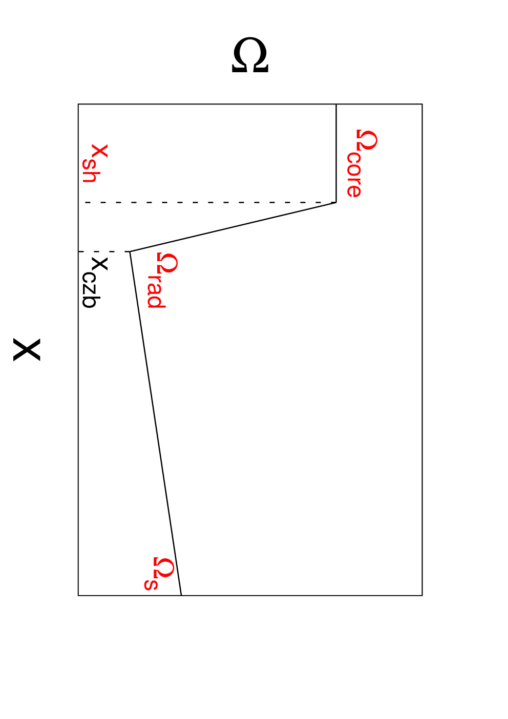
where $\Omega_{0}(x)$ can have a linear profile described with two parameters, namely, the rotation rate at the center $\Omega_{\mathrm{c}}$ and that at the surface $\Omega_{\mathrm{s}}$ (see the blue line in Figure 1) or can have a velocity shear (with four parameters, namely, the rotation rate below a velocity shear boundary $x_{\mathrm{sh}}$ which is assumed to be uniform at $\Omega_{\mathrm{core}}$, the rotation rate $\Omega_{\mathrm{rad}}$ at another side of the shear boundary fixed to be the convective core boundary ($x_{\mathrm{czb}}\sim 0.045$), and that at the surface $\Omega_{\mathrm{s}}$) (see Figure 7).

Another function $\Omega_{1}(x)$, which is related to the latitudinal dependence of the internal rotation, can be zero everywhere (with no parameters) or can have a linear profile (with two parameters, in almost the same way as a linear profile of $\Omega_{0}(x)$ but with additional indices as $\Omega_{1\mathrm{c}}$ and $\Omega_{1\mathrm{s}}$). We have taken such latitudinal dependence of the internal rotation into account in order to evaluate the effect on the global likelihood though it is not a primary subject to be investigated in this study. We note that the final inference on the convective-core rotation is not qualitatively changed due to the inclusion of the latitudinal dependence of the rotation in the analysis as we see later in Section IV.3.

With the definitions for $\Omega_{0}(x)$ and $\Omega_{1}(x)$, there are four ways of parameterization of the rotational profile in total. Let us denote the models as follows: $M_{\mathrm{1d2p}}$ for linear $\Omega_{0}$ and zero $\Omega_{1}$, $M_{\mathrm{1d4p}}$ for shear $\Omega_{0}$ and zero $\Omega_{1}$, $M_{\mathrm{2d4p}}$ for linear $\Omega_{0}$ and linear $\Omega_{1}$, and $M_{\mathrm{2d6p}}$ for shear $\Omega_{0}$ and linear $\Omega_{1}$, where the subscripts $\mathrm{d}$ and $\mathrm{p}$ stand for the dimension of a modeled rotational profile and the number of parameters in the model, respectively (Table 2).

Then, what we have to specify is the corresponding priors for the parameters. As described in Section III.2, each prior probability for a certain parameter is assumed to be uniform as below:

and

The parameters representing rotation rates are in units of $2\pi\times 0.01\,d^{-1}$, and $q\sim U[a,b]$ means that $q$ is a random variable uniformly distributed in a range from $a$ to $b$, as described in Section III.2. The joint prior probability is computed by taking products of the prior probabilities based on the assumption that the parameters are statistically independent of each other.

For each way of parameterization, the posterior probability of the parameters is computed based on the likelihood of the parameters and the joint prior probability. The likelihood is calculated with expressions () and (4). We carry out the so-called Metropolis method (Metropolis et al. 1953), which is one of the standard algorithms to carry out MCMC, to evaluate the posterior probability. The convergence of samples generated via the Metropolis method has been checked by visual inspection (see Figure 8) with several different sets of initial values for the samples. A typical number of iterations required is of the order of $10^{5}$, and small fractions of samples are discarded from the final samples as they are considered as samples in the burn-in periods (a period during which obtained samples are not thought to be realizations from the posterior probability distribution we would like to sample). More information on principles of MCMC, how to manage the outcomes of MCMC, and so on, can be found, for example, in Gregory 2005.

We consider that the posterior probabilities have been successfully sampled via MCMC, based on the convergence of MCMC samples (see Figure 8). Then, we compute the global likelihood for each way of parameterization of the rotational profile to carry out the Bayesian model comparison. Note that the global likelihood $p(\mathbf{d})$, which is the normalization constant in relation (2), cannot be determined with the MCMC samples alone. We therefore need some tools to compute the global likelihoods. This can be accomplished by following the procedures proposed by Chib and Jeliazkov 2001 in which an exact value of the posterior probability of a particular set of the parameters is directly evaluated, and then, the global likelihood is calculated based on relation (2). We have confirmed that the method correctly works for simple cases where we can analytically compute the posterior probability and the global likelihood.

The decimal logarithm of the odds ratios thus obtained are $\mathrm{log}\,O_{M_{\mathrm{1d4p}},M_{\mathrm{1d2p}}}=4710$, $\mathrm{log}\,O_{M_{\mathrm{1d4p}},M_{\mathrm{2d4p}}}=4090$, $\mathrm{log}\,O_{M_{\mathrm{2d6p}},M_{\mathrm{1d2p}}}=5390$, and $\mathrm{log}\,O_{M_{\mathrm{2d6p}},M_{\mathrm{2d4p}}}=4770$ (Table 2), clearly indicating that the rotational profiles with the velocity shear ($M_{\mathrm{1d4p}}$ and $M_{\mathrm{2d6p}}$) are more favored than those without the shear ($M_{\mathrm{1d2p}}$ and $M_{\mathrm{2d4p}}$). The validity of the computation of the global likelihoods has been checked with several different settings in MCMC, and the global likelihoods have been rounded to no more than four significant figures (Table 2).

We can also confirm that based on the posterior probability for the models with the velocity shear, the fast-core rotation is again inferred. Figure 9 shows the 2-dimensional contour map of the (marginalized) posterior probability density function as a function of $(\Omega_{\mathrm{conv}},x_{\mathrm{sh}})$, which is computed for the model $M_{\mathrm{2d6p}}$. Note that $\Omega_{\mathrm{conv}}$ is used instead of $\Omega_{\mathrm{core}}$ to describe the latitudinally averaged rotation rate of the convective core. When we adopt the Maximum A Posteriori estimates for the parameters, they are $(\Omega_{\mathrm{conv}},x_{\mathrm{sh}})\sim(13.4,0.0493)$, and thus, the fast-convective-core rotation has been inferred as in the case of Hatta et al. 2019 (see Figure 8 for $\Omega_{\mathrm{s}}$ and $\Omega_{\mathrm{rad}}$, which are of the order of $1$ in units of $2\pi\times 0.01\,d^{-1}$ and are much slower than $\Omega_{\mathrm{conv}}$).

Since the models used for Bayesian model comparison in the last section are much more complex than those in Section III, we would like to check whether we can conduct Bayesian model comparison even with such complex models, which eventually enables us to validate the results obtained in the last section. To this end, we present the same test as that described in Section III except for the following two points. Firstly, the Maximum A Posteriori estimates for the parameters, which are determined with the posterior probability given the model $M_{\mathrm{2d6p}}$ (computed in the last section), are used for constructing an artificial rotational profile and the corresponding rotational shifts. Let us call the artificial rotational shifts $\delta\omega_{\mathrm{2d6p}}$. Secondly, to compute the posterior probabilities given the artificial rotational shifts, we have used the four models, namely, $M_{\mathrm{1d2p}}$, $M_{\mathrm{1d4p}}$, $M_{\mathrm{2d4p}}$, and $M_{\mathrm{2d6p}}$ (see the definitions of the models in Section IV.2). What we would like to check is whether we can correctly choose the right model ($M_{\mathrm{2d6p}}$ in this case) among the models based on the global likelihoods or not.

The global likelihoods have been computed via the method of Chib and Jeliazkov 2001. The decimal logarithm of the resultant odds ratios are as follows: $\mathrm{log}\,O_{M_{\mathrm{2d6p}},M_{\mathrm{1d2p}}}=20540$, $\mathrm{log}\,O_{M_{\mathrm{2d6p}},M_{\mathrm{2d4p}}}=14390$, and $\mathrm{log}\,O_{M_{\mathrm{2d6p}},M_{\mathrm{1d4p}}}=668.4$ (Table 3). It is therefore evident that the correct model $M_{\mathrm{2d6p}}$ is preferred to the other models from the Bayesian perspective. This can be also confirmed when we see Figure 10, where the prepared parameters (represented by red dotted lines in the figure) can be estimated with little biases only if we choose the correct model $M_{\mathrm{2d6p}}$ (see $\mathrm{P}_{\mathrm{2d6p}}$ in the figure).

Based on the results obtained in Section IV.3, it has been inferred, via the Bayesian scheme, that the convective core of KIC 11145123 is rotating approximately $\sim 10$ times faster than the other regions of the star. We have also confirmed the validity of the results in Section IV.4. In this section, we have a brief discussion about the inferred position of the velocity shear.

Figure 11 shows the Brunt-$\rm{V}\ddot{a}is\ddot{a}l\ddot{a}$ frequency of the reference model (black curve) and the inferred position of the velocity shear (blue dashed line). What we would like to point out is that the inferred position of the velocity shear $x_{\mathrm{sh}}\sim 0.05$ is slightly above the convective boundary $x_{\mathrm{czb}}\sim 0.045$, at which the square of the Brunt-$\rm{V}\ddot{a}is\ddot{a}l\ddot{a}$ frequency is zero, and that the shear is located in the overshoot zone (represented as the blue shaded area in Figure 11). In the overshoot zone, where overhooting has been modeled as a diffusive process following Herwig 2000 in the case of the reference model, the square of the Brunt-$\rm{V}\ddot{a}is\ddot{a}l\ddot{a}$ frequency is positive so that the overshoot zone is included in the g-mode cavity. This is fairly relevant to the inversion analysis since not only the mixed-modes but also the high-order g modes should also have sensitivity for the fast-core rotation (compare the black curve and the orange curve in Figure 12).

The relevance described in the last paragraph can be actually confirmed by a test, in which the Bayesian rotation inversion is carried out without the mixed-mode rotational shifts. We then have the following odds ratio in the decimal logarithmic scale: $\mathrm{log}\,O_{M_{\mathrm{1d4p}},M_{\mathrm{1d2p}}}=20$, (Table 2). Note that the latitudinal dependence is not considered here for simplicity. Although the difference in the global likelihoods are much smaller than those computed with the mixed modes included in the analysis, we can still claim that the model with a velocity shear $M_{\mathrm{1d4p}}$ is more favorable in terms of the global likelihood; the inference of the velocity shear has just become more marginal.

The same analysis with the artificial rotational shifts $\delta\omega_{\mathrm{sh}}$ in Section III.2 has shown that it becomes rather marginal to distinguish the two models of rotational profile (one with a velocity shear ($M_{\mathrm{sh}}$) and the other without it ($M_{\mathrm{lin}}$ )) if we exclude the mixed modes. The odds ratio expressed in the decimal logarithm is $\mathrm{log}\,O_{M_{\mathrm{sh}},M_{\mathrm{lin}}}=1.25$. This is mainly because we artificially locate the position of the shear identical to the convective core boundary and there are no modes which are sensitive to the artificially generated fast-convective-core rotation other than the mixed modes. However, in the case of KIC 11145123, high-order g modes can be sensitive to the fast-core rotation which slightly invade the radiative region, possibly leading to the marginal preference to the model with a velocity shear $M_{\mathrm{1d4p}}$ despite the absence of the mixed-mode rotational shifts in the analysis.

References

- Aerts et al. (2010) Aerts, C., Christensen-Dalsgaard, J., Kurtz, D. W. 2010, AA Library, “Asteroseismology”
- Aerts et al. (2019) Aerts, C., Mathis, S., Rogers, T. M. 2019, Annu. Rev. Astron. Astrophys., 57, 35
- Backus and Gilbert (1967) Backus, G. E. Gilbert, J. F. 1967, Geophysical Journal, 13, p.247
- Beck et al. (2012) Beck, P. G., Montalban, J., Kallinger, T., et al. 2012, Nature, 481, 55
- Benomar et al. (2009) Benomar, O., Appourchaux, T., Baudin, F. 2009, AA, 506, 15
- Benomar et al. (2015) Benomar, O., Takata, M., Shibahashi, H., et al. 2015, MNRAS, 452, 2654
- Benomar et al. (2018) Benomar, O., Bazot, M., Nielsen, M. B., et al. 2018, Science, 361, 1231
- Bradley et al. (2015) Bradley, P. A., Guzik, J. A., Miles, L. F., et al. 2015, ApJ, 149, 68
- Cantiello et al. (2014) Cantiello, M., Mankovich, C., Bildsten, L., Christensen-Dalsgaard, J., Paxton, B. 2014, ApJ, 788, 93
- Chib and Jeliazkov (2001) Chib, S. Jeliazkov, I. 2001, Journal of the American Statistical Association, 96, 453, Theory and Methods
- Christophe et al. (2018) Christophe, S., Ballot, J., Ouazzani, R.-M., et al. 2018, AA, 618, A47
- Deheuvels et al. (2020) Deheuvels, S., Ballot, J., Eggenberger, P., et al. 2020, AA, 641, A117
- Di Mauro et al. (2018) Di Mauro, M. P., Ventura, R., Corsaro, E., et al. 2018, ApJ, 862, 9
- Eggenberger et al. (2017) Eggenberger, P., Lagarde, N., Miglio, A., et al. 2017, AA, 599, A18
- Fuller et al. (2019) Fuller, J., Piro, A. L., Jermyn, A. S. 2019, MNRAS, 485, 3661
- Gizon et al. (2016) Gizon, L., Sekii, T., Takata, M., et al. 2016, Science Advances, 2: e1601777
- Gregory (2005) Gregory, P. C. 2005, Bayesian Logical Data Analysis for the Physical Sciences: A Comparative Approach with Mathematica Support (Cambridge University Press)
- Hatta et al. (2019) Hatta, Y., Sekii, T., Takata, M., Kurtz, D. W. 2019, ApJ, 871, 135
- Hatta et al. (2021) Hatta, Y., Sekii, T., Takata, M., Benomar, O. 2021, ApJ, in press
- Herwig (2000) Herwig, F. 2000, AA, 360, 952
- Jackiewicz (2020) Jackiewicz, J. 2020, SoPh, 295, 137
- Jeffreys (1998) Jeffreys, H. 1998, The Theory of Probability (3rd ed.), Oxford, England, p. 432
- Kashyap et al. (2021) Kashyap, S. G., Das, S. B., Hanasoge, S. M., et al. 2021, ApJS, 253, 47
- Koch et al. (2010) Koch, D. G., Borucki, W. J., Basri, G., et al. 2010, ApJL, 713, L79
- Kurtz et al. (2014) Kurtz, D. W., Saio, H., Takata, M., et al. 2014, MNRAS, 444, 102
- Li et al. (2020) Li, G., Van Reeth, T., Bedding, T., et al. 2020, MNRAS, 491, 3586
- Maeder (2009) Maeder, A. 2009, Physics, Formation and Evolution of Rotating Stars (Berlin: Springer)
- Metropolis et al. (1953) Metropolis, N., Rosenbluth, A., Rosenbluth, M. 1953, J. Chem. Phys., 21, 188
- Mosser et al. (2012) Mosser, B., Goupil, M. J., Belkacem, K., et al. 2012, AA, 548, A10
- Ouazzani et al. (2019) Ouazzani, R.-M., Marques, J. P., Goupil, M-J., et al. 2019, AA, 626, A121
- Papics et al. (2017) Pápics, P. I., Tkachenko, A., Van Reeth, T., et al. 2017, AA, 598, A74
- Ricker et al. (2014) Ricker, G. R., Winn, J. N., Vanderspek, R., et al. 2014, SPIE, 9143, 20
- Rogers (2015) Rogers, T. M. 2015, ApJL, 815, L30
- Saio et al. (2015) Saio, H., Kurtz, D. W., Takata, M., et al. 2015, MNRAS 447, 3264
- Saio et al. (2021) Saio, H., Takata, M., Lee, U., et al. 2021, MNRAS, 502, 5856
- Schmid and Aerts (2016) Schmid, V. S., Aerts, C. 2016, AA, 592, A116
- Schunker et al. (2016a) Schunker, H., Schou, J., Ball, W. H. 2016a, AA, 586, A24
- Schunker et al. (2016b) Schunker, H., Schou, J., Ball, W. H., Nielsen, M. B., Gizon, L. 2016b, AA, 586, A79
- Tayar and Pinsonneault (2013) Tayar, J., Pinsonneault, M. H. 2013, ApJL, 775, L1
- Tikhonov and Arsenin (1977) Tikhonov, A. N. Arsenin, V. Y. 1977, Solutions of Ill-Posed Problems. Winston, Washington, DC
- Townsend and Teitler (2013) Townsend, R. H. D. Teitler, A., 2013, MNRAS 435, 3406-3418
- Unno et al. (1989) Unno, W., Osaki, Y., Ando, H., Saio, H., Shibahashi, H. 1989, Univ. Tokyo Press, “Nonradial Oscillations of Stars”