headingsoptiontoheadandtoc \KOMAoptionlistoftoc,leveldown \KOMAoptionbibliographytoc \addtokomafontsubparagraph
twoside=false
On the performance and programming of reversible molecular computers
‘Engines of Parsimony’
Hannah Amelie Earley
March 2021
This thesis is submitted for the degree of
Doctor of Philosophy,
and was supervised by
Gos Micklem
in the
Department of Applied Mathematics and Theoretical Physics,
and
Trinity Hall,
of the
.
.
twoside=false
This thesis was also advised by
Stephen Eglen,
and was examined internally by
Sebastian Ahnert
and externally by
Michael P. Frank
on the
30th of April, 2021.
to Ann, reunited with Dennis, and to Jim, who we and Patsy yet miss
| Acknowledgements |
| Gos, without whom none of this would be possible; |
| your guidance, identical sleep schedule, and tangents |
| have got me through this path ig-noble. |
| P.S. I forgive you for trying to kill me with peanuts. |
| Mum and Dad, you gave me life, |
| and helped me through my toil and strife, |
| not to mention my sisters three, |
| whose love and kinship supported me. |
| My office-mate Pete(r), |
| I miss our late-night pizza |
| and basketball sessions; |
| may MIT sustain your passions. |
| Swaraj, though you moved to Oxford, |
| your dependability never wavered; |
| your friendship is immeasuarable, |
| and willingness to read my drafts inexplicable. |
| Acknowledgements |
| Georgeos, in but a year of your acquaintance, |
| fast friends we have become; |
| though I have exploited it for articular comments, |
| fast friends I hope we go on. |
| Marianne, who accompanied me through much of my journey; |
| even though our relationship may not have survived the PhD, |
| I may not have survived the PhD if not for you, |
| for which you have my gratitude. |
| My office-mate subsequent Jiaee, |
| who cyclically accompanied me to Ely: |
| about the distance, you and Eleanor lied to me, |
| nonetheless, around your upbeat attitude is fun to be. |
| Finally, these acknowledgements would be incomplete, |
| wihout mentioning the bodies whose funding replete |
| upon me bestowed; DAMTP, Trinity Hall |
| and EPSRC, I thank you all. |
Declaration
This thesis is the result of my own work and includes nothing which is the outcome of work done in collaboration except as declared in the Preface and specified in the text. It is not substantially the same as any that I have submitted, or, is being concurrently submitted for a degree or diploma or other qualification at the University of Cambridge or any other University or similar institution except as declared in the Preface and specified in the text. I further state that no substantial part of my thesis has already been submitted, or, is being concurrently submitted for any such degree, diploma or other qualification at the University of Cambridge or any other University or similar institution except as declared in the Preface and specified in the text. It does not exceed the prescribed word limit for the relevant Degree Committee.
Variants of the core chapters of this thesis, id1, id1, id1 and , have been posted as preprints [earley-parsimony-i, earley-parsimony-ii, earley-parsimony-iii, earley-aleph]. This thesis is my own work, though I will exercise nosism throughout. This work was supported by the Engineering and Physical Sciences Research Council, project reference 1781682 [wearley-ukri].
Hannah Earley11 1 h.earley@damtp.cam.ac.uk, orcid.org/0000-0002-6628-2130
December 2020
Abstract
If the 20th century was known for the computational revolution, what will the 21st be known for? Perhaps the recent strides in the nascent fields of molecular programming and biological computation will help bring about the ‘Coming Era of Nanotechnology’ promised in Drexler’s Engines of Creation [drexler]. Though there is still far to go, there is much reason for optimism. This thesis examines the underlying principles needed to realise the computational aspects of such ‘engines’ in a performant way. Its main body focusses on the ways in which thermodynamics constrains the operation and design of such systems, and it ends with the proposal of a model of computation appropriate for exploiting these constraints.
These thermodynamic constraints are approached from three different directions. The first considers the maximum possible aggregate performance of a system of computers of given volume, , with a given supply of free energy. From this perspective, reversible computing is imperative in order to circumvent the Landauer limit [landauer-limit, szilard-engine]. A result of [frank-thesis] is refined and strengthened, showing that the adiabatic regime reversible computer performance is the best possible for any computer—quantum or classical. This therefore shows a universal scaling law governing the performance of compact computers of , compared to for conventional computers. For the case of molecular computers, it is shown how to attain this bound. The second direction extends this performance analysis to the case where individual computational particles or sub-units can interact with one another. The third extends it to interactions with shared, non-computational parts of the system. It is found that accommodating these interactions in molecular computers imposes a performance penalty that undermines the earlier scaling result. Nonetheless, scaling superior to that of irreversible computers can be preserved, and appropriate mitigations and considerations are discussed. These analyses are framed in a context of molecular computation, but where possible more general computational systems are considered.
The proposed model, the -calculus, is appropriate for programming reversible molecular computers taking into account these constraints. A variety of examples and mathematical analyses accompany it. Moreover, abstract sketches of potential molecular implementations are provided. Developing these into viable schemes suitable for experimental validation will be a focus of future work.
Chapter Introduction
In recent years, unconventional forms of computing ranging from molecular computers made out of DNA to quantum computers have started to be realised. Not only that, but they are becoming increasingly sophisticated and have a lot of potential to influence the future of computing. In this work, we will look at the intersection of molecular computing and another interesting class of unconventional computer: that of reversible computers.

Molecular Computation
The field of Molecular Computation began in 1994 with Len Adleman’s proof-of-concept use of DNA [adleman] in the solution of the classic Hamiltonian path problem, as illustrated in Figure 1. DNA and other nucleic acids proved an apt choice for building molecular/chemical computers, due to its information bearing capacity and the strong preference that single strands show for binding to complementary sequences, not to mention the low cost with which it can be synthesised and analysed as well as the large body of knowledge available from decades of biochemical research. Inspired by Adleman’s paper, a community of researchers designing and building DNA computers arose in concert with the DNAX (and shortly thereafter, the complementary FNANOX) series of conferences22 2 https://isnsce.org/conferences/.
DNA, or deoxyribonucleic acid, is a family of polymeric molecules that is employed by all known organisms to store their genomic information, amongst other uses. Each molecule can be characterised by its sequence: a string of the monomers adenine (A), cytosine (C), guanine (G) and thymine (T). These monomers are each bound to a deoxyribose sugar molecule, which are joined together by phosphodiester bonds. Whilst this ability to store information through the arbitrary combination of these monomers is advantageous, the key to its success is the special hydrogen-bonding properties that these monomers possess. When two DNA strands are aligned adjacently, if adenine and thymine are opposite each other they will be perfectly positioned to form two favourable hydrogen bonds; similarly, if cytosine and guanine are opposite each other they will be perfectly positioned to form three favourable hydrogen bonds. Whilst other combinations may also form hydrogen bonds, the positions are suboptimal and thermodynamically unfavourable when compared to the pairs A-T and C-G. In nature, DNA is found almost exclusively in double-stranded form, whereby each strand has a sequence complementary to the other: if one strand has sequence GGCACAACGT then the other will have sequence CCGTGTTGCA. These complementary strands then hybridise to one another. In fact, this is an oversimplification: in addition to their information content, DNA molecules have an intrinsic orientation, conventionally notated via the free 5’ phosphoryl and 3’ hydroxy groups on the terminal ribose sugars. DNA strands bind anti-parallel, and so the sequences should be written 5’-GGCACAACGT-3’ and 5’-ACGTTGTGCC-3’. Schematically, this looks like
but in reality the strands twist together into a double helix, the structure of which was found by Rosalind Franklin, James Watson and Francis Crick [wc-dna]. Eponymously, the characteristic complementary ‘base pairing’ is known as Watson-Crick base pairing. The DNA computing motifs designed by Adleman and others make use of this Watson-Crick base pairing, but exploit partial hybridisation and the dynamics and interactions of single-stranded DNA.


Whilst Adleman’s proof of concept required manual actuation of each step of the computation, and was limited to NP-complete problems, schemes demonstrating universal computation and autonomous operation were soon developed. An example from the first of the DNAX series is the proposed DNA and restriction enzyme implementation of a Turing Machine of [rothemund-tm]. Whilst universal in principle, it was still not autonomous and has never been experimentally realised due to its complexity. Nevertheless, successful approaches and motifs employing both DNA and enzymes have been developed, such as the PEN toolbox of Yannick Rondelez’s group [pen-toolbox] and the PER reaction of Jocelyn Kishi [per]. Arguably the most popular approaches in the field are enzyme-free approaches. Two famous examples are given by the Tile-Assembly Model (TAM), introduced by Erik Winfree [winfree-tam], and DNA-strand displacement (DSD) schemes, first popularised by Georg Seelig et al [dsd]. These are illustrated in Figure 2.
Some impressive feats have been achieved, from neural networks [qian-nn, cherry-nn] to cargo sorting robots [cargo-sorting] to reprogrammable iterative binary logic circuits [woods-21]. Nevertheless, DNA computing is not without its challenges. For example, DSD systems often exhibit spurious ‘leak’ reactions, and optimisation and tricks are required to mitigate this [leakless-dsd]. Moreover, traditional DSD systems occupy the entire reaction volume, which can therefore only perform a single computation. Strictly speaking, one could perform multiple computations by using orthogonal DNA sequences such that a set of DNA species performing one computation doesn’t interact with another performing a different computation; however, toeholds typically can’t be much longer than 6 nucleotides in length to ensure reversibility of association, limiting the set of distinct toeholds to . Worse still, it transpires that DNA’s sequence specificity is not absolute, and so only a fraction of this design space is useful: in fact, as a single mismatch or two does not prevent hybridisation but does affect the rate of hybridisation, it is often exploited for tuning kinetics [dsd-kin-i, dsd-kin-ii, dsd-kin-iii, dsd-kin-iv]. We have not even mentioned the influence of palindromic sequences and other motifs manifesting non-trivial secondary structures. This seriously limits the complexity that can be realised in these systems, because the CRNs that are compiled into DSD schemes (using, e.g., VisualDSD [visual-dsd]) do not make use of complexation of CRN species, and therefore each sub-module in a program requires a fresh set of CRN species with their own unique DNA sequences—even if the sub-module is identical to another, just used in a different place in the program. Additionally, these DNA computers are analogue which significantly limits their computational complexity if one wants to be certain of the result [crn-probab], although if one is comfortable with slightly less certainty then better complexity is possible [winfree-dna-crn-univ]. They are also very slow, taking on the order of several hours or even days to progress. The tour-de-force examples of neural networks [qian-nn] and (4-bit) square rooting [qian-sqrt], for example, took on the order of 10 hours to converge to an answer.
If instead one makes use of localisation, as with the TAM, then much of these issues with DSD can be avoided [chatterjee-localised]: localising DSD species to a surface allows ‘circuits’ to be constructed which are fast, modular, and can reuse sequence domains. The problem is that constructing these is substantially more difficult than free-solution DSD, and that gate strands are ‘consumed’ during computation making these one-shot reactions. Free-solution DSD also consumes its gate strands, but at least in this case it is possible (if non-trivial) to continually supply fresh gate and fuel species and remove waste complexes. The TAM does not get off completely unscathed either, and methods to suppress errors to mitigate its share of problems have also been developed [tam-err].
This is not to say that computing with molecules such as DNA is intrinsically flawed, but the difficulties in overcoming these issues has left many in the field pessimistic about initial beliefs that DNA could be used to perform arbitrary computation in an effective manner. Instead, the general consensus is that DNA computing may be best used to perform small logical calculations as part of a synthetic biological system. My view is more optimistic, in that I believe that an as-yet undiscovered DNA computing motif exists that will solve all these problems simultaneously. Whilst perhaps the existence of such a panacea is wishful thinking, I believe that the abstract molecular schemes discussed in Sections 19 and lend evidence to this view, and developing these further will be the subject of future work.
Reversible Computation

The problem is that this process requires the dæmon to learn information about the state of the gas particles. In effect, the entropy has simply moved from the state of the particles to the state of the dæmon’s memory. No entropy reduction has occurred. Moreover, eventually her memory will be filled up, and she will likely want to ‘erase’ it to continue her task. Forgetting all this information will correspond to moving the entropy into the state of another system. If this entropy now manifests as heat, then Landauer showed that discarding a quantity of information requires the production of heat where is Boltzmann’s constant, the temperature, and with equality only in the limit of a thermodynamically reversible process (i.e. taking infinite time).
As mentioned, the other class of unconventional computer we shall consider is that of reversible computers. Reversible computers impose the requirement that all state transitions be invertible, and therefore conserve information. The reason for this restriction is that the laws of physics, as far as is currently known33 3 This includes quantum mechanics; the Schrödinger equation specifies that the time evolution operator is unitary and hence invertible. Furthermore, it seems that even the supposedly irreversible process of wavefunction collapse is in fact a reversible one of progressive decoherence, as espoused by the Many-Worlds Interpretation [mwi]., are fundamentally reversible. In contrast, conventional computers are irreversible in the sense that they do not conserve information and that it is not generally possible to deterministically wind back the state of computation. This has surprising consequences: from a thermodynamic perspective, it transpires that this loss of information manifests as a commensurate increase in entropy, whilst from a quantum perspective, the loss of information of some quantum state necessarily results in decoherence of any quantum state entangled with said state. This quantum mechanical behaviour is not of great concern in classical computers, but is untenable for quantum computers and hence they must necessarily be programmed reversibly.


Expanding more on the entropic manifestation of information loss, simulating the ability to discard information in a reversible setting touches deeply on the connection between thermodynamics and information theory, and was formalised by [szilard-engine, landauer-limit]in the twentieth century in order to resolve Maxwell’s eponymous thought experiment, the Maxwell Dæmon (Figure 3). For every bit of information discarded, a commensurate entropy increase of at least is produced elsewhere, where is Boltzmann’s constant. Physically, the information is encoded into environmental degrees of freedom, and this information promptly decorrelates with the original computational system. This decorrelation is effectively irreversible, and hence the information becomes entropic. More generally, whenever a quantity of information is discarded, an entropy increase of manifests, with equality only in the limit of thermodynamic reversibility in which the discarding process takes infinitely long. If this entropy were allowed to remain in the computational system, it would eventually accumulate to such an extent that it would interfere with the well ordered operation of the computational mechanism. As a visceral example, should the entropy take the form of heat, where is the system temperature, the system will eventually transmute into a form incompatible with its function—such as melting or turning into a plasma—as the temperature becomes too great. Even if the system is physically heat-resistant, the increased entropy will result in errors so frequent that almost all the computational capacity is directed to error correction, slowing productive computation to a crawl.
At room temperature, this heat generation will be on the order of per bit discarded. Conventional computers typically expend a factor of around times this much for reasons relating to reliability, speed, and the relatively large size of their transistors in comparison to the atomic scale. It is somewhat challenging to precisely quantify this overhead as the information processing capacity of a modern consumer processor is difficult to ascertain, due to the extensive use of pipelining, vectorisation and multiple-instruction dispatch. Nevertheless, we can obtain a reasonable estimate. arm’s processors are well known for emphasising power efficiency, and are used extensively in mobile electronics as well as some laptops and desktops (notably, three of Apple’s new device lineup). Considering arm’s A-78 processor micro-architecture [arm-a78], we find numbers of around , with each core running at a clock speed of and executing up to per clock cycle with a width of up to . Taken together, these give an energy dissipation of roughly . In contrast, at a temperature of around , Landauer’s bound gives just , a overhead for the arm processor. Intel’s chips have thermal design powers typically exceeding , but have compensatingly greater vectorisation widths of some instructions, such that a similar Landauer overhead can be achieved when fully exploiting the processor’s capabilities.
The origin of irreversibility in conventional computers can be subtle, but it is in fact ubiquitous. This may be considered to ultimately originate in early mathematical models of computations such as the Turing Machine and Lambda Calculus in which overwriting and discarding, respectively, are implicit to the primitive operations of the models. At the lowest levels of abstraction of modern computers, semiconductor logic gates and buses are operated in an irreversible manner: somewhat oversimplifying, traditional CMOS-style logic dissipates energy every time the transistor states switch, and during each clock cycle an equilibration process occurs in which the nodes of the circuit are connected to bus lanes at various reference voltages and any transient voltage disparity is eliminated. Both of these processes are capable of discarding information in the system, although exactly where in these processes the information erasure should be attributed is a non-trivial matter. In fact it is possible to drive CMOS-style logic gates adiabatically [crl, sl-crl, s2lal], achieving asymptotically zero dissipation in the limit of infinitely slow switching. This is assuming that the instructions are logically invertible, perhaps subject to certain pre- and post-conditions in which case it is sometimes referred to as conditionally reversible. Reintroducing irreversibility is possible, but dissipation of information should be performed separately to maintain adiabaticity in the operation of the logic gates. The idea of using reversible logic gates in irreversible computation may seem counter-productive, but it is a useful potential way to make substantial gains in energy efficiency and to get closer to the Landauer bound.
At higher levels of abstraction potential sources of information erasure include the obvious, such as overwriting/mutating a variable, to the less obvious such as variables going out of scope or ignoring a function’s return value. Even more subtly, any iteration or recursion which does not maintain a record of its initiation condition as well as its termination condition is in fact irreversible, as shall later become clear.
With such ubiquitous application of information-destructive primitives, it is hard to see how algorithms can be rewritten reversibly. Indeed, whilst Landauer could envisage what logically reversible logic gates might look like, even describing [landauer-limit] what would eventually become known as the Toffoli or CCNOT gate (see Figure 4), he came to the conclusion that one would end up having to manually keep track of the lost information thus rapidly filling the computer’s memory with useless ‘garbage’ or ‘history’ data. 12 years later, Charles Bennett—often considered the ‘Father of Reversible Computing’—developed a remarkably simple algorithm [bennett-tm] (Figure 5(a)) for embedding any irreversible function as the reversible injection without producing any net garbage. Later, he extended this algorithm [bennett-pebbling] to reduce the amount of interim garbage data produced via a recursive application of the original algorithm, the general principle of which is illustrated in Figure 5(b).


With the viability of reversible computing proven, the stage was then set for more faithful programming of reversible computers to be demonstrated beyond simple injective embedding of irreversible programs. Whilst Bennett did introduce the idea of a Reversible Turing Machine, arguably the first description of a reversible computer that might be physically realisable was given by [fredkin-conlog]. Fredkin and Toffoli introduced conservative logic, in which the number of 1 bits (and optionally also the number of 0 bits) is conserved; they proceeded to show that this logic could be implemented by a system of ideal elastic ‘billiard balls’, projected across an ideal frictionless surface decorated with ideally rigid walls. The motivation for this construction was that it is precisely the sort of system considered by classical mechanics. If one could build such a billiard-ball computer, then aside from the initial kinetic energy supplied to the system, there would be no need to supply additional energy nor any dissipation; moreover, one could recover the kinetic energy at the end for amortised-free computation. To illustrate the principles of billiard-ball computation, Andrew Ressler’s implementation of a Fredkin gate is shown in Figure 6. Going further, Ressler designed an entire reversible computer processor—complete with arithmetic logic unit—within the billiard-ball scheme for his Master’s thesis [ressler], demonstrating that not only were reversible computers theoretically as capable as irreversible ones from a Turing universality perspective, but that they were also practically as capable.
Unfortunately, Bennett’s analysis of the billiard-ball model showed it to be impracticable as a fully dissipationless model of reversible computation:
“Even if classical balls could be shot with perfect accuracy into a perfect apparatus, fluctuating tidal forces from turbulence in the atmospheres of nearby stars would be enough to randomise their motion within a few hundred collisions. Needless to say, the trajectory would be spoiled much sooner if stronger nearby noise sources (e.g., thermal radiation and conduction) were not eliminated.” — [bennett-rev]
We shall have more to say about this in id1, but since then a number of adiabatic designs of classical reversible computers have been developed and experimentally verified, not to mention the recent progress in building quantum computers. We highlight the Pendulum Instruction-Set Architecture (PISA), first introduced by [pendulum] and later refined by [frank-thesis, pendulum2]. This architecture was successfully realised adiabatically with semiconductors by employing the ‘Split-Level Charge Recovery Logic’ (SCRL) motif [sl-crl], as shown in Figure 7. Adiabatic reversible computers achieve far lower dissipation than irreversible computers, but still dissipate energy at a rate inversely proportional to the time per operation. Questions of whether or not lower energy dissipation, or even the ‘holy grail’ of fully dissipationless computation, are achievable have continued to be asked44 4 Such as at the recent 2020 Physics and Engineering Issues in Adiabatic/Reversible Classical Computing Visioning Workshop., and we believe we have answered these in the negative in id1.


Programming Reversibly
With such ubiquitous application of information-destructive primitives, it is hard to see how algorithms and programs can be rewritten reversibly. In we shall introduce a model of reversible computation appropriate for Brownian computers such as the molecular computers discussed earlier, in addition to many examples illustrating the principles of programming reversibly. Learning to do so requires a paradigm shift in one’s thought process, in much the same way as an imperative/procedural programmer undergoes when learning a functional programming language for the first time. Reversibility as a concept is orthogonal to other language paradigms such as imperative/procedural, functional, and declarative, and indeed examples of reversible languages exist for each of these (we believe the -calculus and alethe, introduced in , constitute the first example of a reversible declarative language).
To program reversibly takes some care. At a high level, one must ensure that each block (whether a function, a subroutine, a loop, a conditional branch, a statement, etc) is information preserving: that is, there must be a bijective map between the set of legal inputs and legal outputs. We say legal, because it is possible for some inputs to not map to outputs and vice-versa, instead producing a logical error during execution or entering an infinite loop. For example, consider Bennett’s embedding protocol applied to the factorial function. This would produce a reversible program performing the map , e.g. . If, however, one attempted to feed in the output and run this program backwards then an error55 5 If we assume this is implemented on an RTM, then the error occurs when reversing the copy step: tapes 1 and 3 are initialised to 4 and 30 respectively, then the irreversible factorial TM is run forwards on tapes 1 and 2 to obtain 24 and some entropic garbage; the RTM then attempts to consume the copy of 24 on tape 3, but and so the machine will either stall or its state may become corrupt and meaningless. would occur because there is no input mapping to this output. Once one has ensured that a block is information preserving, the next step is to try to decompose it into smaller information-preserving blocks, just as with regular programming. Expertise with this comes with practice, and my experience with reversible programming leads me to believe that it is possible to become just as proficient with reversible programming as with irreversible. Whilst programming reversibly is to be preferred where practicable, a useful ‘trick’ for implementing a difficult bijection can be achieved by first writing irreversible programs for and , embedding these using Bennett’s algorithm as and , and then constructing the composition .

Arguably the most challenging concepts to learn are those of reversible control flow: conditional branching and loops. Provided the information used to discriminate the different cases in a branch is available before and after, then this branching is clearly reversible. The problem comes when merging these branches later: in irreversible languages this merging of control flow is implicit, but in a reversible language we must ensure that we are able to tell from which branch we came immediately after merging and so merging must be made explicit. In fact, reversibility provides an elegantly symmetric solution to this without introducing a new primitive for merging. The idea is that merging is simply branching in reverse, and so one reuses the branching primitive and supplies a set of orthogonal conditions that must be satisfied by each branch of the computation before control is merged. If the information used to perform the original branch is preserved, then the original conditions can be reused; it is not necessary that the final conditions be the same as the initial, however, and this can often be used for good effect when data is transformed to a different—but provably isomorphic—representation. A loop is similar to a two-branch conditional, except that instead of the execution direction on both sides being in the same direction, they are in opposite directions in order to produce a loop. The consequence is that effectively the entry to a loop is a merge of control flow: one must know whether a loop iteration is being entered for the first time, or as a continuation, so that on reversal it is possible to ‘un-enter’ the loop. The termination condition remains the same as in the irreversible case: at the end of each iteration, it is checked whether we should continue looping or exit the loop. These principles are illustrated abstractly in Figure 8, more concretely in Figure 9, and more extensively in .
We conclude with a brief review66 6 In some code snippets, notation of some arithmetic expressions and operators has been slightly modified where it is thought that the medium of mathematical typesetting provides greater clarity than the ASCII source. of some (classical) reversible programming languages.
(Janus)
To our knowledge, the first such programming language—Janus—was designed by [janus] in 1982 for a Caltech class project, and later formalised by [janus-analysis]. It is an imperative procedural language, and is named after the Roman god associated with duality and time. Listing 10 illustrates most of its syntax through three increasingly sophisticated examples, or see 0.1 for a more detailed exposition.
[t].27
[t].32
[t].41
The first example (due to [janus-analysis]), fib, is a recursive procedure which computes the and Fibonacci numbers into and respectively, consuming in the process. The second (due to us), fac, is an iterative procedure that replaces with (providing ), using as a ‘scratch’ variables for implementing and to hold the burgeoning factorial as is consumed. The third (due to [janus]), sort, performs a bubble sort on the list of length , and sets to the permutation mapping between the original and sorted lists (as a precondition, must be set to the identity permutation ). The absence of dynamic-length arrays or memory allocation (and hence use of 99 as a fixed buffer size in the above) shows a limitation of Janus, though the augmentation of Janus to support such features would be a straightforward extension.
Definition 0.1 (Syntax and semantics of Janus).
A program consists of a series of (global) variable declarations and procedure declarations. Variables are either machine-precision integers, initialised to 0, or fixed-length arrays thereof as indicated by the square brackets. Variables are modified by in-place updates, or can be swapped with . There are three possible in-place operators, , and (in-place bit-wise XOR), and the right-hand side of a statement can be any compound expression making use of the unary operators (arithmetic negation), (bit-wise negation); the arithmetical binary operators , , , (quotient), (remainder); the bit-wise binary operators , , ; or the Boolean binary operators , , , , , where False is represented by 0 and True by . These expressions need not be information-preserving, as the semantics make use of a Bennett embedding: computing in the forward direction the value, performing the modification, and then uncomputing the value. As a result, it is illegal for the variable being modified to appear in the expression modifying it.
Procedures can be called in their forward direction by the aptly-named statement, and in their reverse direction by . Janus also supports conditionals and looping, per the aforementioned principles. Conditionals are represented by . They consist of a branch and unbranch condition, respectively and , and optional statements to be executed in the True () and False () cases. If evaluates to True before the branch, then must evaluate to True afterwards, and similarly for the converse, or else a run-time error occurs. Loops are similarly defined, represented by . Upon reaching a loop, must evaluate to True. The statement(s) , if any, are then executed. Then is tested; if it evaluates to False then the statement(s) are executed, else the loop exits. Otherwise, is evaluated once again (and must this time evaluate to False), and execution continues from . Not described here are the rudimentary I/O operations and Janus run-time system.
(-Lisp)
A little while later, in 1992, Henry Baker introduced two Lisp variants: Linear Lisp [linear-lisp] and -Lisp [psi-lisp]. The former employs linear logic [linlog], in which every value must be consumed precisely once (usage optional), in order to do away with expensive garbage collection in functional languages. This idea is seeing a resurgence, with support in recent updates to languages like Haskell [linear-hs]. Whilst linear logic shares some properties with reversible computation, indeed quantum logic is often contextualised as a subset of linear logic, it is not restrictive enough to guarantee reversibility. Baker’s etymologically-palindromic -Lisp, however, does guarantee injectivity of its primitives and is therefore reversible. It is itself a variant of Linear Lisp appropriately modified. The most conspicuous modification is that of the -expression. Baker introduces the merge condition in an asymmetrical way, as the return value is not necessarily named: the first two sub-expressions are, respectively, a Boolean expression indicating which branch to take, and a Boolean predicate to be applied to the result. These predicates are handled specially, in comparison to the rest of the language, in that they are permitted to be non-invertible. As with expressions in Janus, these predicates are run forwards to select a branch, and then backwards to erase the garbage. Unfortunately the paper is somewhat lacking in precise detail of the language design, and so it is not clear how one defines new predicates (other than the mention of an implicitly instantiated history stack created when these predicates are evaluated), nor is it clear what happens if a predicate is called outside of such a scope.
To showcase the syntax and semantics of -Lisp, [psi-lisp] provides a reference implementation of the factorial function (reproduced in Listing 11). Unfortunately, this definition is not reversible as it is not possible, given output 24, to mechanically invert the expression to obtain . In fact this is not a failure of the reversibility of -Lisp, but rather a failure to adhere to the principles of linearity: is used twice in this expression! Moreover, the presumed definition of is not invertible or possible. This demonstrates the ease with which one can introduce a bug when programming reversibly, although were an interpreter/compiler for -Lisp available it would surely not accept the proposed program.
In Listing 12, we attempt to provide a corrected -Lisp implementation of the factorial. This implementation is an iterative loop disguised in recursive form, as it does not appear that tail-recursion is possible in a reversible context due to the loss of information pertaining to recursion depth. The original paper is somewhat light on details, and so this definition is somewhat speculative, particularly with regard to user-defined predicates: here we define an auxiliary function first-onep which returns whether its first argument is 1 or not, and assume the existence of a primitive to access the implicit history stack. We also (reasonably) assume an invertible implementation of in which evaluates to , although the linearity restrictions in -Lisp mean we must refer to the output by a different name than the input . The parameter tracks recursion depth, increasing from an initial value of to a maximum of , whilst is simultaneously decremented from to 1. As we retrace our steps, we multiply by the depth counter , and then decrement , such that when we finally return from fac the depth counter has been restored to its initial value (e.g. 1). The wrapper function fact handles supplying and consuming this depth counter, and assumes that -Lisp permits pattern matching on constants or some other way to consume a known constant.
( R R)
Another language with Lisp-like syntax, R R (“yar”), was introduced in 1997 by [frank-r]. However, unlike -Lisp, the language is procedural and C-like—using the Lisp-like syntax for convenience of implementation (which is written in Common Lisp). To the best of our knowledge, this is the first, and perhaps only, (classical) language for which a compiler targeting a reversible processor exists; namely, the aforementioned Pendulum Instruction-Set Architecture (PISA). Indeed, the example program in Listing 13 was compiled to PISA assembly and executed on an emulator (though, to our knowledge, not on a physical PISA implementation such as Pendulum).
Semantically, R R is not dissimilar to Janus, but it does support local variable scoping which makes it more powerful as a structured programming language. On the other hand, it does not (as of 1999) possess the ability to have different conditions on entry and exit for conditionals and loops, nor does it appear to support unbounded loops. Nonetheless, such features can be simulated and so this is not a fundamental limitation of the language.
The example in Listing 13 begs some further discussion. The Schrödinger equation was first discretised in a reversible way by [schro-rev]. It has the remarkable property that, although its update rule is in some sense inexact, it nevertheless conserves amplitude (observed by Fredkin and proved by Feynman). To understand the example, we first briefly sketch how the Schrödinger equation, which describes the time evolution of the wavefunction under the action of the Hamiltonian , may be discretised. This equation has the formal solution ; this is formal in the sense that is an operator, which in common formulations takes the form of a Hermitian matrix or a partial differential operator, and so some care must be taken when manipulating it. Supposing we wish to use a timestep , we can write for any value of . It may be more convenient to supply the program with , having also pre-discretised such that is a matrix and a vector, in which case the simulation can be performed exactly and reversibly77 7 It may be observed that matrix multiplication for non-singular (which is, being unitary) may be performed reversibly using Gaussian-elimination. Specifically, applying the row reduction algorithm to yields where is the identity matrix. As is unitary, computing its inverse is trivial (the inverse of a unitary matrix is its conjugate transpose).. Here, however, the program receives . Specifically, we are considering a one-dimensional cyclic potential well in which , and the value of the potential is supplied at each discretised point. Expanding for small and discretising space, we find
Here the approaches of Fredkin and Frank differ; Frank identifies that the real part of the wavefunction at the next timestep is only informed by the imaginary part of the wavefunction at the previous and vice-versa, in order to use this directly. In contrast, Fredkin seeks a more symmetric approach, transforming this to a form : in this form the reversible implementation is more obvious without needing the observation of real-imaginary orthogonality, but one must retain copies of the wavefunction at two timepoints instead of the one in Frank’s version. With the discretised Schrödinger equation thus derived, Frank’s program is a simple transcription of this (after performing the routine algebra to discriminate the real and imaginary parts) with the array corresponding to and to the coefficient (twice the phase rotation per time-step due to the particle’s kinetic energy). It also assumes space has been discretised 128-fold. Finally we comment on the operator which indexes into an array, and the operator , peculiar to R R, which returns the upper 32 bits of the 64-bit product of two 32-bit signed integers (the purpose being to implement the rounded product of an integer with a fixed point number in ).
(Kayak)
Perhaps marking the debut of reversible programming into public perception, Ben Rudiak-Gould introduced Kayak in 2002 as an entry [kayak] for the second instance of the Esoteric Awards (‘Essies’). The Essies are an annual competition in design and use of esoteric programming languages. Esoteric programming languages are not targeted for real-world use but instead are experiments in designing languages that may, for example, be intentionally difficult to program in or are very minimal whilst remaining Turing complete. The most well-known esoteric language is Brainfuck (BF), created in 1993 by [brainfuck]. As well as being known for being hard to program in (though certainly not the most difficult, the honour of which arguably goes to Malbolge [malbolge]), its syntactic minimalism and semantic simplicity make BF attractive for proving Turing-completeness of new languages and indeed the original distribution of Kayak included a BF-to-Kayak compiler (as does our language, alethe, introduced in ).
Definition 0.2 (Syntax and semantics of Kayak).
Kayak has very few primitives. A program is a series of procedures, each consisting of a bipartite name (e.g. ), an input and output set of -delimited variables (these sets should be of equal length), and a body. Procedure bodies can contain one of four ‘commands’: variable invocation, temporary register negation, conditional execution and procedure invocation. Variables are infinite stacks of bits, and invoking a variable will pop the top-most bit and place it in the ‘temporary’ register if this register is empty, otherwise it will empty the temporary register onto the top of the named stack. The temporary register is local to procedure bodies and conditional blocks. Variables not named in the inputs/outputs are also local to procedure bodies (but not conditionals), and are initialised to an infinite number of 0s (and should be restored as such upon procedure exit). If the temporary register is occupied, then the command will negate its bit. The command is a conditional block, which will run the nested commands if and only if the temporary register is occupied and set to 1. Finally, a procedure can be invoked by calling its bipartite name with some variables; for example, will swap the contents of the stacks and . Procedures can be run in reverse by reversing their names; for example, a factorial calculated using the program in Listing 14 can be un-calculated by calling . Of course, if a name is palindromic then its reverse is inaccessible, and so it is recommend that only self-inverse procedures have palindromic names. A fascinating property of this syntax is that inverting a program is as simple as reversing the characters of its file and mirroring the characters .
Kayak seems inspired by BF in terms of its syntactic obscurity, as may be gleaned from 0.2. Nevertheless, it is possible to write useful programs in it as we demonstrate in Listing 14 with an implementation of the factorial function. In fact, the algorithm employed is much the same as that we used in Listing 12. Moreover, we also provide88 8 https://github.com/hannah-earley/kayak/blob/master/arith.kayak convenience routines for the reading and writing of base-10 ASCII representations of numbers, thus showing that the presence of modular abstractions—even in a language as cryptic as Kayak—permits arbitrarily complex programs to be readily written. In keeping with its obscure intention, we also provide a ‘golfed’ variant in Listing 15.
(‘YAG’)
Whilst -Lisp went some way towards the construction of a functional reversible programming language, its incomplete definition leaves it unclear whether this was achieved—not to mention that Lisp-esque languages are not deemed to be ‘pure’ functional languages. In 2012, [yag-lang] introduced a language—hereafter referred to as ‘YAG’—which seems to meet the criterion of being a functional language. The example of computing Fibonacci numbers from the paper is reproduced in Listing 16, and the semantics are summarised in 0.3.
Definition 0.3 (Syntax and semantics of ‘YAG’).
Like most functional languages, ‘YAG’ is expression oriented. A primary difference, however, is that function application may only occur in and expressions; this increased indirection helps enforce the reversibility of the semantics. These expressions take the form where and are what we shall call99 9 In the original paper, these are called left-expressions by analogy to the common understanding of left-expressions in language syntaxes, however the occurence of left-expressions on the right-hand side of the equals sign is somewhat confusing. patterns, is a function name, and an expression in which to substitute the bindings of . The form runs forwards with input , and the runs backwards with output . A pattern is either a variable, e.g. , a constructor applied to some number of sub-patterns, e.g. the Peano numbers would be encoded inductively by the forms and , or the special ‘duplication’ pattern (where , , etc are syntactic sugar for the tuple constructors , , etc). The ‘duplication’ pattern is unique1010 10 Duplication and equality testing as concepts are of course not unique to ‘YAG’, but the particular place this concept holds in the syntax and semantics is a seemingly novel feature. to ‘YAG’; for a full explanation, the paper [yag-lang] is the best source, but essentially reduces to whilst reduces to if , else to , and thus by matching on these two forms via a expression, equality can be tested (and exploited to un-copy in a safe way). The remaining expression form is given by , where the body defines some number of branches . Here also ‘YAG’ takes a slightly different approach from other languages in this space. Whilst most languages require that the potential matching patterns be orthogonal, in ‘YAG’ this is not the case; instead, the first pattern matching the input selects the branch taken. Similarly, once the branch returns an output from , this must be unique only amongst the expressions in contrast to most other languages where it must be unique amongst all the expressions. Finally, a program is a series of function definitions of the form .
(Theseus)
The last language we will review is Theseus, whose name is inspired by the legendary Ship of Theseus in that its computation ‘[replaces] values by apparently equal values’. Based on the family of point-free1111 11 Point-free languages do not support explicit variable binding, instead modelling computation as ‘flow through pipelines’; a point-free approach can often be used to elegant effect, and in languages supporting a mixed approach such as Haskell this is encouraged. Honourable mentions in this space are the languages Inv and Fun of [inv-lang], whose motivation was in developing a language for bi-directional transformations. Bi-directional transformations are another thread in the field of reversible computation, useful for such applications as editors in which there is an isomorphism between the (editable) document description and the resultant document view. combinator calculi introduced by Roshan James for his graduate thesis [pi-calc], [theseus] introduced an equivalent higher level language. The motivation for is to provide a Category-Theoretic underpinning of reversible programming: specifically, corresponds to dagger symmetric traced bimonoidal categories. Category Theory has long been a source of fruitful cross-fertilisation between the realms of mathematics and computer science, with monadic effects in Haskell a prime example. The typical direction is to attempt to find a category that models an existing programming language, such as Hask1212 12 The familiar reader will object that Hask is not, strictly speaking, a category due to the interaction of the primitive seq with bottom values. for Haskell; Theseus goes the other direction, deriving a language from a category. The objective of this is as an aid to reasoning about categorical constructions rather than to produce a useful language as such, nevertheless a reference interpreter exists1313 13 Mirrored at https://github.com/hannah-earley/theseus.
Definition 0.4 (Syntax and semantics of Theseus).
Theseus is based on type isomorphisms, and has the strongest and most developed type system of those reviewed here. A Theseus program is a series of type definitions and isomorphism (‘map’) definitions, and its syntax largely resembles a subset of Haskell’s. A map is defined by a name, a type isomorphism, an optional name for its inverse, and a series of pattern clauses. Unlike in Haskell, either side of a pattern clause may invoke an isomorphism; if an invocation occurs on a ‘target’ side then it will be called and its return value substituted, as expected, if it occurs on the ‘matching’ side, however, then its inverse will be called and the result then matched. There are two further extensions to maps. Firstly, maps may be parameterised in order to simulate higher-order isomorphisms (this is just a simulation, as maps are not first-class values in Theseus). Secondly, maps may have typed ‘labels’, syntactically represented by where is its appropriately typed argument. The function of labels is as a sort of ‘go-to’ operator. Implicitly a map with type and label types and is transformed to a map . Then, the map is called repeatedly (‘traced’) until it returns a value of type and can thus be used to implement looping. For example, if such a labelled map yields a loop of 3 iterations, then we would call the modified map four times on and then match on the output, i.e. . A core difference between this language and the others reviewed here is that the clauses of a map must not only be orthogonal, but also exhaustive. This complicates definitions of even something as simple as adding 1 to a natural number, because the output of add1 cannot be 0; to circumvent this, explicit divergence of these cases must be employed, i.e. introducing an infinite loop.
The semantics of Theseus are summarised in 0.4 and illustrated in the example implementation of Fibonacci numbers in Listing 17. In Listing 17, the definitions of trace, addSub, add1 and add are due to [theseus] whilst the remaining definitions, cantorUnpair, fib’ and fib, are due to us1414 14 The original paper also supplies a definition of fib, but as a Bennett-esque embedding.. The aforementioned exhaustivity requirement makes this substantially more complicated than, e.g., that in Listing 16 because we must manufacture an exhaustive handling of the error condition. In fib this is very prominent because the subset of corresponding to valid Fibonacci pairs has vanishing measure. Additionally, we attempt to reduce the extraneous cases by internally operating on . James and Sabry do suggest at the end of their paper that it may be possible to extend Theseus with more conventional error handling, which we believe would be the more optimal choice for a programming language. Explicit divergence has a number of downsides in our opinion: from a programmer perspective, coding up divergence conditions is quite cumbersome1515 15 We would estimate it occupied of our time in constructing the fib example!, and there is no ‘correct’ choice of how to do so as these cases are meaningless, thus making it more of an art than a science. Furthermore, from a user’s perspective this divergence behaviour is sub-optimal as one cannot distinguish a long-running/intentionally non-halting computation from an error condition or bug, not to mention the excessive resultant CPU utilisation. Of course, these objections are besides the point of Theseus, but would serve as a small modification with disproportionate benefit for adoption of Theseus as a viable typed functional language for reversible computation.
We will revisit the matter of reversible programming languages in , but for the next three chapters we shall return to the physics of reversible computation.
In this chapter we will consider the maximum sustained computational performance—in terms of operations per second—that can be extracted from a given region of space, under fairly general assumptions. Namely, we assume the known laws of physics, and that one will need to supply the system with energy over time in order to keep it going. We show, similarly to early work by [frank-thesis], that for any realisable computer reversible computers are strictly better than irreversible computers at any size. We also derive universal scaling laws describing just how much better a reversible computer could be compared to an irreversible computer, proving that the adiabatic Time-Proportionally Reversible Architectures (TPRAs) of Frank are the best possible, and suggest a path to achieving this bound with molecular computers.
To illustrate these results, summarised in Figure 18, suppose we wish to build the most powerful computer we can within some spherical region of space, of radius . If the computer is irreversible, such as conventional silicon-based processors, then it is found that essentially only the surface of this sphere can be used for computation and the interior must be empty or inert. This clearly limits the rate of computation proportional to . The reason for this restriction is thermodynamic, arising from constraints on both supply of power and rejection of heat. If is very big, such that the computer threatens to collapse into a black hole, then it is found that the computational rate can now only scale proportional to .
For a reversible computer the situation is substantially improved. In principle, a reversible computer can operate without producing an increase in entropy and without requiring any input of energy, and so the rate of computation could scale with the volume. Unfortunately in practice this is not possible, and a more careful consideration of the system’s entropy is required. The rate of computation is found to scale proportional to , geometrically between the area and volume. For large , general relativistic effects become significant and this falls to the more restrictive bound . For even larger this eventually falls to proportional to , coinciding with the irreversible computer. The reason for this additional threshold between scaling laws is that the sub-relativistic reversible computers—where gravitational effects on spacetime are negligible—are not taking full computational advantage of their volume due to thermodynamic constraints; as the system gets larger beyond the collapse threshold (when the geometry transitions to a thick shell rather than a sphere) the thermodynamic constraints gradually relax, allowing a scaling that ‘temporarily’ exceeds the limit value of .
Therefore we see that at almost all scales, reversible computers substantially outperform irreversible ones, whilst at extremely small—typically sub-nanometer—and large—order of the visible universe in size—scales they coincide.
Chapter Limits on Computational Rates in Physical Systems

reversible computers at absolute zero; reversible computers at finite temperature; irreversible/canonical computers; critical density (thick shell on the cusp of gravitational collapse); critical density (thin shell on the cusp of gravitational collapse).
1 Introduction


The ubiquity of computer technology—and the increasing demands set upon it by intensive algorithms from fields such as machine learning, physics simulations, and cloud computing, among others—render the question of computer performance of considerable interest. Perhaps the most well known observation on computer performance was published by [moore-law], who noticed the trend of microchip component density doubling every 18 months, later dubbed ‘Moore’s law’ in his honour. This law seemed to apply to many quantities in computing, including clock speed, FLOPS1616 16 FLOPS, or FLoating point Operations Per Second, is a common measure of supercomputer performance. of the top 500 supercomputers combined, and inverse storage cost. A popular debate arose over when, if ever, Moore’s law would stagnate; for clock speed, this point has come and gone, with consumer processor clock speeds frozen around .
Whilst it is not surprising that contemporary technology may pose limits on computational performance, it is pertinent to ask whether the laws of physics impose hard bounds on performance. Indeed, our knowledge of quantum physics, thermodynamics and relativity reveals the answer to be affirmative, as hinted at in the introduction chapter. For a brief overview of some of these constraints see, for example, Lloyd’s analysis [lloyd-ultimate].
In this chapter, we investigate how these bounds vary as a given computational system is scaled up. The results we find apply, with different constants of proportionality, for any given computational architecture. A computer constructed from a mix of architectures can be treated as a linear combination, and therefore these scaling results apply to any computer. This builds upon the work of [frank-thesis], proving that his notion of adiabatic Time-Proportionally Reversible Architectures (TPRAs) are the best possible, confirming the relevant scaling results in the mesoscopic regime (as well as analysing scaling in very small and very large regimes in more detail), and excluding the possibility of architectures of lower dissipation. Moreover, the detailed calculations herein yield specific constants of proportionality for broad classes of reversible computational architectures.
There are many metrics by which one may wish to measure computational performance. In this chapter, we shall investigate ‘speed’ as defined by the rate of state transitions the computer is able to execute. As we are more concerned with the general form of scaling law rather than the specific constants for a specific architecture, the exact definition of ‘state’ and ‘transition’ are not too important. In general the most ‘obvious’ definitions can be assumed, for example a conventional silicon-based computer would have as its states each possible value of all its registers, memory and any attached storage device, and as its transitions a single machine instruction1717 17 To be specific, we refer to the combination of a single op-code and its parameters.. More rigorous definitions can be found in quantum mechanics, wherein a state would be an eigenstate of the computational basis Hamiltonian, and a transition would correspond to the complete evolution of the state between orthogonal eigenstates.
Other performance metrics of interest might concern synchronisation between distinct computational elements within a parallel system, and interaction with some arbitrary non-equilibrium system such as a supply of additional memory resources. These shall be covered in id1 and id1, respectively.
Quantum Constraint on Computer Performance
As a first approach to bounding computational performance, we turn to quantum mechanics. [bremermann-limit] gave a back of the envelope calculation in 1962, subsequently refined and elaborated upon by [margolus-levitin] and summarised in Figure 19(a), to show that a system with energy can change state at a maximum rate of where is Planck’s constant. Assuming this energy is due primarily to rest mass, this gives . Restricting our attention to a specific architecture as defined earlier, we assume a fixed density—or at least that the density is bounded from above—such that . This immediately implies that the maximum rate of computation scales with volume.
Thermodynamic and Geometric Constraint on Computer Performance
This quantum limit assumes a closed computational system, requiring no external power source. As we saw earlier this is not possible for conventional computing architectures, being irreversible and hence subject to the Landauer bound [landauer-limit, szilard-engine]. To recall, the Landauer bound quantifies the increase in entropy that occurs whenever information is irreversibly discarded into the environment (as must occur when trying to overwrite data or otherwise reset some arbitrary state to a known state). Explicitly, whenever a quantity of information is discarded, an entropy increase of manifests where is Boltzmann’s constant, with equality only in the limit of thermodynamic reversibility in which the discarding process takes an infinite period of time.
In order to sustain computation then, it is necessary to remove the additional entropy at the same amortised rate as its production. In the case of heat, this is achieved by cooling the system; this process can be generalised to other forms of entropy, such as disorder in a spin bath [landauer-spin], but we shall restrict out attention to heat for conceptual convenience. We must thus enact a flow of work into the system and heat out in order to sustain computation, but here we encounter a geometric constraint. This energy flow applies at every bounding surface, assuming that the heat is ultimately rejected to infinity. Consider a convex bounding surface of area , and assume our technology of choice is capable of transporting energy up to a certain flux , then the maximal power that can be exchanged with the system is given by . As has been established, however, the rate of heat generation scales with the rate of computational transitions for an irreversible computer, and therefore the rate of computation is ultimately bounded by the system’s convex surface area, rather than its volume as contended by the quantum mechanical limit. See Figure 19(b) for an illustration.
This is far more restrictive than the volumetric upper bound derived earlier, and suggests that for large computers only a subvolume equivalent to the outermost shell of the volume can perform useful computation with the remaining bulk relegated to dormant inactivity1818 18 The remaining bulk need not be entirely devoid of purpose. It may, for example, be used for storage and memory. It must however have negligible entropy generation, such as that resulting from structural deterioration due to cosmic rays, spontaneous tautomerisation, etc.. That is, we take the more restrictive of the two bounds, which for small systems is the volumetric bound and for larger (irreversible) systems is this areametric bound.
Ballistic Computation
Does this areametric thermodynamic bound render the volumetric quantum bound inaccessible? A trivial exception is found at small scales, where the surface area to volume ratio becomes so large that the volumetric bound is in fact more restrictive than the areametric bound, and thus takes priority. To more robustly improve on the rate of computation, however, we must reduce the entropic cost associated with a computational transition. As was elaborated upon in the introduction chapter, this necessitates conserving information during computation by using the concept of reversible computation. Whilst the utility of reversible computation was initially controversial, with Landauer initially [landauer-limit] believing it to not be useful, it was soon shown by [bennett-tm] that reversible computation was viable. Moreover, he showed how any irreversible program could be efficiently simulated on such a reversible computer without excessive memory overhead, thus proving that reversible computing was equipotent with conventional computing. For a brief exposition of reversible programming, refer back to id1.
An idealised reversible computer would produce no entropy in its transitions. [fredkin-conlog] described such an idealised system, a physical model of reversible computing that could operate without being actively powered. This model consisted of a frictionless table upon which hard elastic billiard balls were projected. The balls would bounce off of each other and some strategically placed walls, with the precise configuration describing the resultant computation. As a testament to its capability, Fredkin’s student, [ressler], proposed the design of a fully programmable billiard ball computer, complete with arithmetic logic unit. See Figure 6 for an illustration of the general principles of the billiard ball model. Given that such a computer would be powered solely by its initial kinetic energy, the volumetric quantum bound would be attainable. Unfortunately, [bennett-rev] calculated that such a design would ultimately be infeasible as even the most distant and subtle influences would be sufficient to rapidly and completely thermalise the motions of the system. Such influences could in principle be suppressed by error correction mechanisms, but error correction corresponds to the discarding of excess entropy, and would seem to reconstitute the very issues we were trying to avoid.
Our last refuge against unwarranted entropic influences is in quantum ground state condensates. Phenomena such as superfluidity and superconductivity arise in a sufficiently cooled system, wherein a macroscopic fraction of particles are found to inhabit their ground state, manifesting macroscopic quantum behaviours and a subsystem with vanishing entropy and temperature. The utility of such systems is manifold, but unfortunately it is doubtful that they can be exploited for dissipationless computation; the reason is that, in order to enact transitions to orthogonal quantum states, the Schrödinger equation requires us to prepare a superposition of (distinct) energy states which then rotates under the action of the Hamiltonian. The presence of non-ground eigenstates will necessarily result in a renewed vulnerability to thermodynamic perturbations. Nevertheless, such cold temperatures are not altogether useless, as unwanted fluctuations would still be significantly suppressed.
Brownian Dynamics
The fluctuations and dissipation that result from these thermodynamic perturbations lead to diffusion of the distribution in phase space, and hence loss of absolute control over it. Consequently there will be some level of unpredictability to the state of the system and its (generalised) velocities. In the limit of negligible control, the dynamics are (mostly) dominated by the noise source; this regime is referred to variously as Brownian or Langevin dynamics. In Section 4 it shall be shown how to leverage the minimal extant control over the system to make net progress, and to even robustly surpass irreversible computers in performance.
Summary
Whilst fully dissipationless computation is all but impossible, it is still possible in principle to tune the system so as to bring the entropic transition cost as close to zero as desired. In exchange, the rate of computation may itself be diminished. In the chapter that follows, this compromise is evaluated across the range of known physics—from quantum to classical, non-relativistic to relativistic—covering the full spectrum of feasible computational architectures. In so doing, a universal scaling limit is discovered, exceeding that of irreversible computers yet still falling short of the volumetric quantum bound.
2 Quantum Ballistic Architectures and the Quantum Zeno Effect
We first consider a quantum architecture. A viable quantum architecture must be ballistic in the sense of following an exact prescribed trajectory in phase space, as to do otherwise would lead to decoherence undermining the computational state. Of course we have established that a ballistic quantum system cannot truly be isolated from entropic effects; in particular, the third law of thermodynamics precludes lowering the temperature of any system to absolute zero, and so we must incorporate a heat bath into our analysis.
Suppose the ballistic Hamiltonian is given by and the perturbative effect of the heat bath by , such that the true Hamiltonian is . Further, let the initial density be and introduce the projector corresponding to the subspace of valid states, such that . To ensure processive computation, we must therefore periodically correct errors introduced by the perturbation. The cost of such error correction will be bounded from below by the entropy increase due to , which can be expressed in terms of the probability of an error corresponding to the erroneous subspace .
If corrections are to be made at intervals , then this error will be found to be . For a time-dependent Hamiltonian, the quantum Liouville equation tells us that where is Planck’s constant. We can expand as
where we have omitted explicit time dependence for brevity and written . We then find
where the last line uses the fact that . Note that if the term vanishes, then so do all higher terms, and therefore this term is always the leading order approximant.
In order to evaluate this trace, we first write and as block matrices in the basis , yielding
Using the idempotence of projectors, i.e. , and the fact , we can see that . Therefore, we have
The first thing to notice about this expression is that it varies with the square of . This is characteristic of the Quantum Zeno Effect (QZE [qze])—that is, in the limit of constant measurement (i.e. ), we can freeze dynamical evolution. Here, we are performing a partial measurement by projecting onto the subspace of either valid or erroneous computational states, thus allowing computational evolution to continue. Of course, the Zeno rate itself is subject to the Margolus-Levitin limit [margolus-levitin] and so such constant measurement is not possible.
To proceed in further determining , and thereby , it is important to elaborate on certain architectural details. Margolus and Levitin’s analysis shows that one gets the same total rate regardless of whether one considers transitions of the system as a whole (‘serial’) or the combined transitions of a system partitioned into subsystems (‘parallel’). For a physically realistic system, measuring large subsystems as a whole is impractical and so a more fine-grained architecture is likely preferable. Nevertheless, we shall proceed generally, finding the result is independent of this detail.
Let the subsystems be indexed by . For a fully serial system, . We allow each subsystem to evolve independently, assuming that interaction events are negligibly frequent relative to our Zeno corrections. Specialising our above result for , we have
The strength of the perturbations will be controlled by an effective temperature for that subsystem, . Suppose the subsystem has degrees of freedom1919 19 Excluding any frozen out by low temperatures., hereafter referred to as computational primitives. By the equipartition theorem, the energies of each primitive will be individually perturbed. For an uncorrelated perturbation, we expect that where is the time-average value of . Therefore, . The expected aggregate perturbation over all primitives, then, is assuming is Gaussian and where is Boltzmann’s constant.
As for the second term, , we expect that on average will mix (near-)degenerate states indiscriminately. represents the probability that the perturbation stays within the intended computational subspace. The state space can be divided into disjoint computational subspaces, within which the dynamics perform a reversible cycle over computational states. Let the total state space have cardinality , and the number of microstates associated with each subspace be where indexes the different subspaces such that . Assuming similar energy distributions between subspaces, the chance of remaining within the original subspace is . We further approximate this by where is the average subspace cardinality. Equivalently, we can define , the number of distinct programs that the subsystem is capable of executing. Therefore,
In fact, we may wish to correct the second term errors in which we jump within the same subspace, as this may interfere with synchronisation between different subsystems (or it may be difficult to ascertain whether we have jumped within the same subspace). In this case, the expression reduces to
In any case, is always finite and for any useful subsystem; that is, a useful subsystem should have . For composite/non-primitive subsystems, we would like the number of useful programs to scale exponentially with the number of primitives, i.e. for some (typically on the order of unity but greater than 1). For a composite subsystem of even moderate size, this exponential scaling will render the term effectively unity.
We are now able to determine the entropy increase between Zeno cycles. The indiscriminate mixing of the perturbation means that, in the event of an error, the entropy attains its maximum value. This yields the following expression for the information entropy2020 20 We use to refer to the information theoretical entropy, connected to the thermodynamical entropy as . Furthermore, we use the lowercase quantity to refer to the entropy of a subsystem or particle.,
This expression assumes ignorance of states within the current computational subspace; again, we may wish to correct these errors too, in which case we may simply substitute . This would effectively lead to taking where , and so the inequality remains valid.
Putting these together, we get
where is the Zeno measurement rate for the subsystem and . The aggregate rate of entropy generation is given by and is subject to the constraint where is the system temperature that governs the Landauer bound and is the heat dissipation power, proportional to the system’s surface area. It may seem surprising that . In fact, this only applies for sufficiently small ; when becomes significantly large, approaches its maximum of .
We wish to maximise the computational rate, subject to this constrained entropy production. Per Margolus and Levitin, this rate depends on the combined energy of the computational primitives. If the average energy per primitive in subsystem is , then the energy available for computation is and the computational rate is subject to .
Introducing the Lagrangian multiplier , we wish to maximise with respect to ;
This gives and so
solving for and summing over ,
where the average is taken over the computational energy distribution and gives the net Zeno rate of the system as a whole. Substituting into the constraint and making use of the fact that ,
where can be called the ‘Szilard’ temperature: the temperature of the system in which entropy is generated and must be subsequently erased. Finally, we obtain an expression for the net computational rate ,
Now, as the upper bound of is proportional to the bounding surface area, and the upper bound of is proportional to the system’s volume, we get the scaling law
consistent with the scaling law for adiabatic architectures found by [frank-thesis] and showing it to be an upper bound.
We note that [levitin-toffoli-full] derive a related expression for the rate of energy dissipation/heat production within a quantum harmonic oscillator (QHO),
where is the probability of error per state transition and is the number of QHO energy levels. Given that their analysis assumes maximal , however, this simplifies to
where is the separation of energy levels. Given that is assumed constant in the analysis, this then yields an areametric bound on . Our analysis permits to vary, and its optimum value as a function of system parameters is obtained. We also remain general in the systems studied, and thus confirm the conjecture that for a fixed error probability the energy-dissipation rate increases quadratically with the rate of computation.
We also note the recent results2121 21 The author gratefully acknowledges Mike Frank for pointing them towards this body of work. of [pidaparthi-lent] on the Landau-Zener effect (LZE) [lze1, lze2]. In a closed quantum system, with no thermal coupling to the external environment, the Landau-Zener effect predicts that the energy dissipation decays exponentially with the switching time of the system (the inverse of the computation rate). That this is non-zero even in the absence of an external environment shows the difficulty in achieving ballistic computation even in ‘idealised’ conditions, but it certainly points towards a route to achieving near-ballistic computation in regimes in which thermal coupling is negligible. As expected, once thermal coupling is re-introduced to the system Pidaparthi and Lent show how the adiabatic behaviour is recovered. Moreover, their numerical results indicate that the LZE does not appear to be a practicable approach to achieving super-adiabaticity, except perhaps in a very narrow region of system conditions and size. Moreover, the results of Pidaparthi and Lent show the occurrence of a local minimum of dissipation with respect to switching time that would lead to engineering difficulties in increasing computer size for this parameter range. In any case, our asymptotic results stand, although it would be instructive to characterise the parameter range in which the LZE is exploitable and in which the aforementioned engineering difficulties arise.
3 Classical Architectures I: A General Lagrangian Approach
If use of the QZE is not possible, perhaps because of high temperatures or an excessive Zeno rate, then Fermi’s golden rule applies, giving . Consequently —and thus —is subject to a finite lower bound. We find , yielding . Combining with our constraint , the inequality in becomes
where here is Planck’s constant, and so the scaling law falls to . That is, any ballistic system not making use of the QZE will be subject to the same areametric limit as irreversible computers.
The breakdown of the QZE corresponds to an increase in thermal coupling. By abandoning the desire to maintain well defined quantum states, we instead enter the incoherent regime of the classical realm wherein quantum effects are significantly suppressed. Proceeding generally, we adopt a Lagrangian formalism in order to remain noncommittal in our choice of coordinates .
We introduce a reasonably general Lagrangian, ,
where the coefficients , , … may depend continuously on the coordinates , and Einstein notation is used for repeated indices. We have rewritten the Lagrangian in matrix form for concision, where is a matrix, a scalar, a row vector, and a column vector. We assume the system is (effectively) closed, self-contained, or otherwise independent of its environment, and thus will not formally depend on the time parameter. In addition, this property implies invariance under global translation of any of its coordinates and thus conservation of all associated momenta. We obtain the Hamiltonian and generalised momenta thus
Notice that the terms of our potential linearly dependent on the velocities drop out of the Hamiltonian. Those dependent on the cube or higher remain, but will turn out to be negligible at the velocities optimal for computation (and are typically not physically relevant in any case).
For brief collisions, the change in coordinates is negligible and so the spatiotemporal variance in coefficients can be neglected. In this case, we should conserve the Hamiltonian and momenta. We introduce superscripts to the coordinates, , to represent different particles. We also introduce notation for the velocities before, , after, , and their change, . For a collision between particles and ,
where we use the fact that is symmetric. Substituting into , we find,
where is the generalised reduced mass of the system. We can solve for , and thereby , by rewriting thus,
This form reflects the fact that we lack sufficient constraints to unambiguously solve for the post-collision picture. In Cartesian coordinates for point particles, this manifests as an unknown direction of motion afterwards. This is usually resolved by introducing the constraint that momenta perpendicular to the normal vector between the colliding bodies are unchanged. In our generalised coordinate system, the appropriate constraint is unspecified. The general solution is given by
where is a unit vector of unknown direction. We now find an expression for the change in kinetic energy of our particle of interest, ,
where we have introduced a factor to take into account our uncertainty in the final direction, and where we have assumed . Being more careful, we can determine thus,
where is the average of prior velocities, weighted by their generalised masses , and is another uncertainty factor related to . When is large compared to , . When it is small, . Thus a better approximation to is given by
gives the energy lost from the computational particle to some environmental particle , and thus is the amount of energy that must be supplied to the computational system and dissipated from the thermal system. In order to proceed we must determine the rate of this energy transfer; if we assume that the kinetic dynamics of the system are significantly faster than the computational transitions, as suggested by our inability to sufficiently control the quantum state, then we can assume negligible extant correlations between the positions and velocities of different particles. Thus we can employ a kinetic theory approach to determine this rate.
We first determine the mean free path , the average distance a particle travels between collisions. Given the vanishing correlations, we are able to treat collisions between different species of particle separately. For spherically symmetric particles, we find for the mean free path of particles between collisions with particles, where is the number density of particles. More generally, we can replace with , the effective collision cross-section for arbitrarily shaped particles averaged over impact orientation. We also need to determine the average relative speed between and particles,
where we have used the fact that the velocities are uncorrelated to cancel the cross term. Summing over these rates for each class, we can find the rate of loss of kinetic energy for particles,
When particles are heavy and fast, this reduces to
where is the generalised density. Notice that this takes the same form as the equation for hydrodynamic drag, taking the drag coefficient to be . Assuming there exists some correspondence between the generalised velocity and the rate of computation, we find
where ranges over computational particles and is the characteristic generalised displacement corresponding to a single computational transition. To maximise the net computational rate , we find that we need to let , but this violates our assumption that particles are fast. For finite velocity computational particles, we thus find that our net computational rate scales as .
In the limit of slow particles, , instead reduces to
where we have taken . If the generalised mass of the particles is not significantly heavier than the particles, then will have a strong dependence on and this will lead to the same scaling limit of . In order to improve on this, we must let the particles be significantly heavier. In this limit, and we get
To proceed, we maximise the rate subject to this power constraint,
where is the total number of computational particles. To maximise the computational rate , then, we let scale with the volume of the system, leading once again to the scaling law
4 Classical Architectures II: Brownian Machines
Whilst the previous two sections should suffice to cover all physical computational systems, the high mass-low speed limit of the classical system is not ideal from an engineering perspective. For improved practicality, we reformulate this limit in terms of an abstract chemical reaction network (CRN) near equilibrium, and show that we obtain the same result. This result is thus more robust in terms of its attainability.
Entropy generation rate
We first seek a general expression for the rate of entropy generation for a chemical reaction network. Consider any such dynamical system consisting of a set of species and a set of reversible reactions , where we sum over and the are stoichiometries. By the convergence theorem for reversible Markov systems, the system will converge to a unique steady state/equilibrium distribution for any initial conditions. As the reactions are reversible, the steady state will also satisfy detailed balance such that the forward and backward rates coincide separately for each reaction, i.e. , where is a rate of the whole system rather than per unit volume.
Let us look for a quantity that measures progress towards equilibrium and satisfies the following properties:
- 1.
is a state function of the system2222 22 More accurately, on the joint state of an ensemble of iid systems., depending only on its instantaneous description;
- 2.
increases monotonically with time;
- 3.
is additive, i.e. for any set of disjoint regions .
By properties 1 and 2 and the convergence theorem, will approach a unique maximum at equilibrium. Microscopically, reactions occur discretely and so the rate of change of can be written
for any reaction , where we have used reversibility to identify and where is the entropy of the region associated with precisely particles of each species . In order to satisfy property 2, the sign of must equal that of .
Now, consider fixing and , and varying ; this is possible unless the reaction is trivial with for all species , i.e. it does nothing. To maintain property 2, it must therefore be the case that . To satisfy property 3, we require where is some arbitrary scaling factor of the system. We can therefore infer the functional form for some constants and .
We have therefore derived an entropy-like quantity, unique up to choice of logarithmic unit via and entropy at via . Without loss of generality we choose and , and therefore find that
where is the effective bias of reaction and is its gross reaction rate.
Entropy generation rate for elementary chemical reactions
We now calculate our entropy quantity for elementary chemical reactions and compare against the expected value. The rates for elementary chemical reactions are given by collision theory as
where and are rate constants and are rates per unit volume. Assuming no inter-particle interactions, the canonical entropy is given by the Sackur-Tetrode equation which can be obtained simply by considering the spatial distribution of the particles along with any other degrees of freedom. For species , consider an arbitrary volume available to it; if the thermal volume of the particles is where is the thermal de Broglie wavelength, then there will be loci available to the particle, and so the associated entropy within the volume will be
where is the number of particles in the volume, and the concentration. We have also taken into account indistinguishability of the particles with the Gibb’s factor, and allowed for additional degrees of freedom with the term. Strictly speaking the spatial distribution should be calculated combinatorially via the multinomial coefficient
where we have assumed all the particles inhabit the same region and have the same wavelength. Applying Stirling’s approximation and assuming that , this reduces to however, so our simplistic derivation is valid.
Therefore we find the canonical entropy change due to reaction is given by
using a slight abuse of notation (the logarithmands are not unitless, but their combination is). Comparing with our quantity , we find
which should be compared to the Arrhenius equation. Indeed, the terms confer the appropriate units to the pre-exponential factor and, by expanding the enthalpy term in terms of as , we can group the roughly constant terms of the enthalpy into the pre-exponential factor, leaving the exponential term in the form .
Maximising performance in Brownian machines
We wish to maximise the net reaction rate of the system by selecting the biases of each individual reaction, subject to bounded total entropy production. If is the total gross reaction rate, then the total net rate is where the expectation value is with respect to the fractional contribution of each reaction, i.e. weighted by . We denote this by assuming that each reaction contributes to computational progress; if this is not true then will be less than this value. The entropy rate is similarly given by . We use a Lagrange multiplier approach as usual,
that is, the optimum is achieved by setting all the equal to a constant, . This gives and hence
leading once again to the scaling limit , as the power scales with area and the gross computation rate with volume. Here we have presented a constructive proof of this scaling limit, as any valid reversible CRN implementation will yield this scaling limit.
5 Relativistic Effects at Scale
At different scales, from the microscopic to the cosmic, different constraints predominate in the analysis of maximum computation rate. For macroscopic systems at worldly scales, the aforementioned thermodynamic constraints are most directly relevant, yielding an upper bound of . At sufficiently small scales, however, the surface area to volume ratio will be great enough that this thermodynamic constraint will no longer be limiting, with the volumetric Margolus-Levitin bound instead dominating. This reflects the fact that there is simply insufficient energy enclosed in the system for the resultant rate of computation to saturate the heat dissipation capacity at the boundary. If one were to use a denser computational architecture, the computational capacity of the region could be increased to the point that the power-flux bound is saturated, and thus recovering the more restrictive bound.
It transpires that there are two further regimes. As our systems approach cosmic scales, the threat of gravitational collapse becomes pertinent. In order to avoid this fate, we must lower the average density such that the system’s radius always exceeds its Schwarzschild radius2323 23 In reality, the threshold radius for gravitational collapse exceeds the Schwarzschild radius by a factor not less than . The reasons for this shall be discussed in due course.. As the Schwarzschild radius is proportional to the mass of the system, this implies that the computational rate of such large systems varies linearly in radius. In fact, there is an intermediate regime: as we have not been utilising the full computational potential of our mass due to the thermodynamic constraint, we can gradually increase said utilisation whilst simultaneously reducing our overall density until the Margolus-Levitin limit is attained, at which point we default to the linear regime. This intermediate regime is thus still described by the limit, which in this post-Schwarzschild realm equates to . In summary, the scaling laws of these four regimes go as , , and , in order of increasing scale.
A more detailed analysis reveals that these large systems are subject to a further consideration. So far we have assumed a Galilean invariance worldview. At small and medium scales, this approximation is very good. At larger scales, however, relativistic effects threaten to reduce our overall computation rate via time dilation, and at even larger scales they can constrain the amount of mass we can fit within a volume lest the system undergo gravitational collapse as mentioned earlier. Special relativistic time dilation is easily avoided by minimising relative motion within the computational parts of the system (this implies that message packets will have reduced computational capacity compared to the static computational background, but message packets can generally be assumed static anyway).
Gravitational time dilation is a more serious issue, which cannot be eluded at large scales. In the case of a hypothetical supermassive computational system, local computation proceeds unabated, but distant users interfacing with the system will observe slower than expected operation, as depicted in Figure 20(a). To calculate this slowdown factor, we shall proceed by modelling the system as spherically symmetric. This is not unreasonable at these scales, where a body’s self-gravitation makes maintaining other geometries unstable and impractical. We will not consider rotational systems which could allow for an ellipsoidal shape, as the requisite angular velocities would almost certainly abrogate nearly all computational progress solely due to special relativistic effects.
The metric2424 24 We use a signature. of an isotropic and spherically symmetric body in hydrostatic equilibrium can be obtained via the Tolman-Oppenheimer-Volkoff (TOV) equation [tov-eqn],
| (1) |
where is the pressure, is the mass enclosed by the concentric spherical shell of radius , and is the local mass-energy density. All masses are as observed by a distant observer.
The rate of dynamics of a point as observed from a point is well known to be
where is the metric tensor. We assume our distant observer to be moving slowly (relative to the computer) in approximately flat space, and thus that . This yields a slowdown factor of . The total slowdown for an extended body is hence found to be
| (spherically symmetric) | ||||
where is the total mass and is the least upper bound of its radial extent.
In order to maximise , we must clearly maximise throughout the body. It can be seen that , and in fact within solid regions where this inequality is strict. Furthermore, in empty space the TOV equation breaks down; instead, we use our Schwarzschild matching conditions to find
which shows that this inequality is always strict whenever . at the surface is fixed by the Schwarzschild metric, in accordance with Birkhoff’s theorem, and thus for a fixed extent our only control over is the distribution between the surface and core. Approaching the core from the surface, strictly decreases until vanishes. Furthermore is at least as great as in empty space, being strictly greater in massive regions. Therefore it is desirable to concentrate mass towards the surface.
We assume that the density of our architecture of choice is bounded from above, thus limiting the degree to which we can concentrate mass towards the surface. The optimum is then achieved by a thick shell of limiting density from the surface inwards. The two extreme cases of a thin shell and a solid sphere can be treated exactly, but an arbitrarily thick spherical shell must be treated numerically.
Solid Sphere
A solid sphere coincides with the Schwarzschild geometry. The usual Schwarzschild metric corresponds to the exterior of the object, instead we must use the interior solution which can be derived from the TOV equation (1), yielding
where is the Schwarzschild radius. Before computing , note that vanishes when . This limit is in fact of great importance; whilst an object of size would exceed the Schwarzschild radius and be presumed stable against gravitational collapse, this is not the case. At this point, such an object is unstable towards spontaneous oscillations, its core pressure diverges, and it readily collapses to a black hole [schwarz-lim-main]. Furthermore, depending on its heat capacity ratio , a gaseous hydrostatic sphere may be unstable at even larger radii as tabulated by [schwarz-lims]. This threshold is thus a stronger bound on the size of massive objects. Integrating over the mass of this solid sphere, we find
where we have introduced the normalised coordinate . At the threshold, we get .
Thin Shell
For a thin shell, we first identify that the pressure on the outer boundary vanishes. Let the inner radius be and the thickness be such that and . We also introduce the unitless variable ,
where . Integrating from the surface inwards, we have and , yielding
Therefore in the limit , the pressure throughout the thin shell vanishes. As a result, we also have that is constant for all , taking the value and giving
At the threshold, we get .
Thick Shell
For general , we integrate numerically. We rewrite the TOV equations in normalised and unitless form thus
where , and . We integrate the system from down to , with initial conditions , and . Our slowdown factor is given by , and explicit results are given in the following section.
6 Variance in Performance at Different Scales
In order to calculate the maximum performance of a system at different sizes, we compute the optimum speed within each constraint—thermodynamic and Margolus-Levitin—with relativistic corrections, and then pick the least of these upper bounds. To apply the relativistic constraint, we substitute for mass where is the Schwarzschild radius, and then multiply by our slowdown factor . For better parametericity, we actually use where is the system’s radius/linear dimension. This yields the two bounds,
where and are constants of proportionality that depend on the system architecture. Notice that there is in fact some choice available in system geometry; we can pick any constant density thick shell solution, with parameters . As we increase , the factor will decrease, and so there will be an optimum pair maximising the given bound. The maximum density constraint is equivalent to setting a maximum value to the mass and hence ,
where the last constraint is to avoid gravitational collapse. For a given then, we have and we maximise the two bounds in .
An illustrative example of these regimes is depicted in . Notice how the solid sphere, though maximising usable computational matter and thus its local computational rate, has its observable computational rate abrogated as it approaches the point of gravitational self-collapse. This demonstrates how reducing the available matter can enable the observable computational rate to increase, though the difference between the dashed and solid lines shows that there remains a relativistic penalty in the form of gravitational time dilation. We also see that an irreversible system underperforms with respect to a reversible system across a large range of length scales, otherwise matching it at the extremes. The exact range again depends on system architecture specifics, and for some architectures the irreversible system may give transient superior performance at certain scales.
7 Discussion
Additional Entropic Sources
The preceding analysis has been restricted to dissipating entropy arising in the course of the computation itself. However, a physical computer will be subject to other sources of entropy in addition to this. As mentioned in the introduction, Bennett calculated that the influence of turbulence in the atmospheres of nearby stars would be sufficient to thermalise a billiard ball computer within a few hundred collisions. Thus, in general, we must aim to shield our computer from such external influences, for example by error correction procedures. Fortunately, the influences of such external sources may only interact with our system via the same boundary through which we dissipate computational entropy, and as such their rate is at most proportional to this surface area2525 25 Even though such external influences may indeed permeate the entire volume, such as gravitational waves or neutrinos, the rate of incidence of these interaction will necessarily scale areametrically. Moreover, gravitational waves and neutrinos only penetrate the entire volume because they are so weakly interacting. A more strongly coupled interaction such as ultraviolet light or particulate matter will primarily affect only the ‘skin’ of the system, and thus illustrates how such external influences are genuinely only areametric in strength.. Thus, as long as the external sources are not overwhelmingly strong we should be able to suppress them at all scales with equal ease.
A more challenging source of errors and entropy comes from within. Assuming a non-vanishing system temperature, the entire system volume will generate thermodynamic fluctuations at a commensurate rate. These fluctuations can manifest in a variety of ways, perhaps the most damaging of which are nuclear transitions. Some nuclear transitions, such as radioactive decay leading to the production of damaging radicals, are not of great concern over long timescales as the proportion of unstable isotopes will decay to zero exponentially fast. More problematic is the tendency of all nuclei to decay to the baryonic ground state2626 26 In fact, the ground state of nuclear matter depends on density, and at higher densities the equilibrium state may be as high as ; beyond this, various forms of degenerate matter may dominate [baryon-ground-state]., [nickel62] (either by fission or fusion); except for systems composed purely of , these spontaneous transitions must be reversed in order to maintain the intended structure. Every event leading to a change in computational state or requiring repair invokes an entropic cost, and given that these events occur with a rate proportional to the computationally active volume, this ultimately recovers an areametric bound to our computational rate,
This does not necessarily render our reversible computation performance gains unattainable, however. Providing is sufficiently small, we can outperform irreversible computers at scales up to
where is the thickness of the irreversible computational shell that can be supported by such an architecture. If this threshold size is sufficiently large as to coincide with the Schwarzschild threshold of then such a reversible architecture would in fact outperform its irreversible analogue at all scales. Furthermore, it is likely that is smaller than it would be in an irreversible system as they have one fewer source of fluctuations to combat; namely, irreversible computers expend significant quantities of energy to ensure unidirectional operation, and any deviation from this is a potentially fatal error. In contrast, a reversible computer is intrinsically robust to such ‘errors’, particularly the Brownian architecture described, which actively exploits this. Expending less energy has the added advantage of permitting lower operating temperatures, further reducing .
Mixed Architectures
Because of the generality of the scaling law, systems of maximal computational rate can be constructed using any desired mix of architectures in order to meet the requirements of a given problem. Providing entropy and input power can be efficiently transported between the surface and the computational bulk, the entropy generation and power constraints superpose linearly. Thus in principle it is possible to have a mix of quantum and Brownian architectures within a single system. A caveat is that these two architectures may need to operate at different temperatures, and a temperature gradient introduces an additional source of entropy. Thus, the area of the boundary between these subsystems must be at most proportional to the system’s bounding area in order that the entropy generated can be effectively countered.
This principle is more general: any non-equilibrium inhomogeneity in the system’s structure will result in entropy generation. To quantify this, we assume that such inhomogeneities equilibrate via an uncorrelated diffusive process, and we proceed via a Fokker-Planck approach.
The Fokker-Planck equation (see Section 10.2 for a more detailed exploration) describes the evolution of a probability distribution in space due to stochastic dynamics. Specifically, it pertains to the influence of a Langevin force with rapidly decaying correlations in time. In this limit, Brownian particles will exhibit a combination of drift and diffusion depending on the properties of the system. The evolution of the probability distribution is found [risken] to obey2727 27 In [risken], the convention is . We use a different convention here for convenience, wherein .
where is a drift vector and is a diffusion matrix. We also identify the probability current . In order to establish the rate of entropy generation, we must first determine the steady state distribution. We make the assumption that the steady state probability current is everywhere zero, i.e. there are no persistent current flows or vortices, and therefore find that
Now we obtain an expression for the entropy of the system. As there are many particles, we can reinterpret as a concentration of particles (as the Fokker-Planck equation does not impose any normalisation), and so each particle will have an associated entropy of where . This yields intensional entropy and . At equilibrium, cannot have a leading order linear term in , and so which gives
We now substitute the Fokker-Planck equation for , obtaining
where is the number of particles of diffusive species . In the second line we have assumed that the probability current across the system boundary vanishes and in the last line we have generalised to multiple diffusive species.
The consequence is that a system may only sustain the use of spatial variation in its architecture if at least one of the following three conditions holds for each such species,
- 1.
The region of variation scales with the system’s surface area, such as if the gradient is localised to a hemispheric plane,
- 2.
The diffusion rate is vanishingly small,
- 3.
The average relative strength of the gradient, , has scaling no greater than .
These conditions may be violated only to the extent that another condition is exploited to achieve a commensurate reduction in the entropy rate.
Modes of Computation
The quantum Zeno architecture is inherently processive, meaning that every transition it makes is useful. This is in contrast to the Brownian architecture, in which only a vanishingly small fraction of transitions lead to a net advance in computational state. There are a number of consequences to this distinction that make the quantum architecture preferable.
Firstly, a quantum architecture equivalent to a given Brownian architecture will only use active computational elements compared to , which significantly reduces the risk of errors due to internal fluctuation. In addition, the properties of the QZE mean that the fluctuations within the computational subvolume of the quantum architecture can be rectified at all scales in contrast to the classical system. Of course, fluctuations in the remaining bulk of the volume are still problematic, but their rectification is less critical.
Secondly, whilst the two systems would have the same net rate of computation, the computational elements of the quantum system operate at the same maximum speed regardless of scale, and the degree of parallelism can be tuned between maximally parallel () and fully serial (). This means that the quantum architecture can operate equally well for parallel and serial problems. One caveat is that the maximal attainable parallelism of the quantum system, , is lower than for the Brownian, . In practice this is not too problematic as parallel problems can be simulated serially, and because the total computation rate is independent of the degree of parallelism, the quantum system experiences no penalty for this choice. For the Brownian system, however, even a problem maximally exploiting the available parallelism will be limited by the time for each element to perform a single net operation. In addition, whilst the quantum system has fewer computational foci than the Brownian system, the remaining bulk can be used for ‘cold’ computation such as data storage.
Thirdly, almost all parallel problems will involve inter-element communication and synchronisation. As will be discussed in id1, these processes present significant challenges in the Brownian architecture that in the worst case would throttle the system down to . This arises because synchronisation processes map to constrictions in phase space, and Brownian diffusion through such a constriction is very slow. As the quantum architecture evolves processively, it is less subject to this effect and thus its computational elements can communicate much more freely.
Fourthly, the quantum architecture permits quantum computation whereas the Brownian architecture is unlikely to be capable of supporting quantum computation. The reason for this is that the average time for each computational transition in the Brownian system is typically large, increasing as the system size does, whereas the decoherence timescale for a quantum state is fixed and typically small. Furthermore, the decoherence timescale is likely significantly smaller than for the QZE architecture as the Brownian system probably operates at a higher temperature. Altogether, these factors make it incredibly unlikely that a quantum state can be reliably maintained through a quantum computation within such an environment.
Despite all these disadvantages, the Brownian architecture is perhaps of more interest as it is ostensibly easier and cheaper to construct with current technology. The most exciting avenue for this may lie in the fields of biological and molecular computing, in which molecules such as DNA are constructed in such a way that their resulting dynamics encode a computational process [winfree-tam, cardelli-dsd]. Chemical systems are a natural substrate for Brownian dynamics, and the manipulation of DNA is becoming ever cheaper and more sophisticated. With improvements in synthetic biology, we may even be able to readily prepare self-repairing DNA computers in the near future.
We finish by discussing the timestep for a net computational transition in the Brownian architecture. This timestep is controlled by the biases, . To maximise the system’s computation rate, we take . If, at operating reactant concentrations, the time for any computational step (forwards or backwards) is , then the net timestep is given by
which can be seen to get larger as the system gets larger. Fortunately this scaling is sublinear, and so depending on the available power, the achievable bias may be significant. For example, assuming a radiative capacity and a radius system consisting of fairly conservative computational particles of size operating at a gross rate of , a bias as high as is possible.
Another approach to managing modes of computation in a Brownian computer is to institute a hierarchy of bias levels at different concentrations. For example, a viable system may consist of the following tuples ,
and computations requiring faster steps may use higher biases at the expense of less computational capacity. Additionally, the highest bias level admits irreversible computation, and so we may enclose our computer with a thin irreversible shell, whilst the internal bulk consists of reversible computations at various bias levels. Going further, we could have a hot inner Brownian core, a cold outer quantum core, and an enveloping irreversible silicon shell. Additionally, a hierarchical Brownian system need not employ spatial variation; by using different species for each bias, the subsystems can be mixed homogeneously.
8 Conclusion
We have shown that, subject to reasonable geometric constraints on power delivery and heat dissipation, the rate of computation of a given convex region is subject to a universal bound, scaling as , and that this can only be achieved with reversible computation. For irreversible computation, this bound falls to . The scaling laws persist at all practical scales, only breaking down when the system size approaches the Schwarzschild scale. For typical densities (), this threshold scale is . Recall that we are considering systems of fixed uniform density; building and maintaining a structure of this density at such sizes may not be practical without some combination of high tensile-strength materials, orbital motion2828 28 Orbital motion near the Schwarzschild regime is not sufficient. For such an object, stable circular orbits only exist for at which point the orbital velocity approaches the speed of light., and propulsion. Beyond this scale, the maximum computational rate is attained by localising mass into as thin a shell as possible, reminiscent of megastructures such as Dyson spheres from the world of science fiction. At very small scales, the rate scales with as the surface area to volume ratio is negligible. The scaling then falls to , to , and finally to as the system increases in size. At the Schwarzschild regime and beyond, the computation rate is suppressed by a factor of order unity due to gravitational time dilation.
This analysis has assumed that each computational element acts independently. In our next two chapters we shall investigate the constraints affecting cooperative reversible architectures, in particular the thermodynamic cost of synchronisation processes, such as communication and resource sharing. These costs turn out to be quite significant, even prohibitive.
In id1, the limits on the sustained performance of large reversible computers were investigated and found to scale as where is the convex bounding surface area of the system and its internal volume, verifying and strengthening a result of [frank-thesis], compared to for an irreversible computer. This analysis neglected, however, to consider interactions between subunits of these computers. In particular, a large computer will be composed of many small computational subunits. Each of these subunits will perform independent computation, but for useful programs one often wishes to combine the results of these independent computations. To do so, the subunits must communicate—they must synchronise their individual states. In an irreversible computer with ample free energy density, this is a non-issue. In contrast, when free energy is limiting, the hidden entropic cost of synchronisation is made manifest and must be considered.
To illustrate, consider two reversible Brownian computers which would like to communicate with one another. A reversible Brownian computer is free to wander back and forth along its configuration space, the set of possible computational states it can take, and we can illustrate this by the analogy of two wagons on intersecting train tracks as shown in Figure 21. In order to synchronise their states, and progress past the intersection, both wagons need to arrive simultaneously. If one wagon arrives before the other, however, then it is almost certain to wander backwards instead of waiting for the other to arrive. If the probability of moving forward is and backward is , then the system is said to have ‘computational bias’ , and the probability that a wagon is at the intersection point is . The rate of synchronisation can then be found approximately by the probability that both are there simultaneously, .
Already the rate of independent computation for each subunit is vanishingly small in the limit of large system sizes, and so synchronisation and communication events in Brownian computers are seen to progress even more slowly and appear to ‘freeze out’ as free energy gets sparser and sparser. In this chapter, we show that there is indeed no way to design a better system for synchronisation of Brownian computers, evaluating the ‘time penalty’ for a synchronisation event across a broad range of possible designs. We also briefly consider the applicability to non-Brownian reversible computers, conjecturing that all reversible computers whose computational elements evolve independently are subject to the same penalty. We conclude with a discussion of design approaches and mitigations to circumvent the synchronisation time penalty in those reversible computers subject to such a penalty.
Chapter Performance Trade-offs for Communicating Reversible Computers


9 Introduction
In id1, we investigated how the laws of physics constrain the maximum rate of sustained computation within a given region of space. In fact, this performance measure of operations per unit time is not the only one of interest. As we are considering computers of arbitrary size, interaction between different subvolumes will often be of considerable import. In this chapter and id1, we evaluate performance within this context. id1 concerns the statistical dynamics of communication between two or more distinct computational units, whilst id1 concerns the statistical dynamics of computational units interacting with resources or chemical species, of which there may be a variable number of identical units or particles. Within these analyses we shall work with Brownian computers as our canonical computational system. Nevertheless, we believe our results are more general, and in the conclusion of this chapter we conjecture upon the classes of reversible computational systems to which our results do and do not apply.
To proceed we must define what we mean by a ‘Brownian computer’. We already introduced a notion of Brownian computer in Section 4 in which we used the formalism of Chemical Reaction Networks (CRNs), but the analyses of id1 and id1 shall require some elaboration. First, it will be helpful to introduce some terminology to distinguish the unique properties of computational particles from those of more traditional chemical species:
Definition 9.1 (Mona and Klona).
A chemical system is generally comprised of a number of species. Each of these species is present at some count; that is, there is some number of particles of this species in the system, and these are identical copies of each other. The study of chemical thermodynamics and statistical mechanics then builds atop this. In contrast, chemical and Brownian computational particles are typically unique within the system: each particle represents the state of some computer, and each evolves independently of one another. It may be that occasionally two or more such particles are transiently identical, but this is a coincidental occasion. An alternative instance of effectively unique computational particles arises in fixed lattices of simple elements, such as in amorphous computers. Here, the elements at each lattice point may not be globally unique, but as they are uniquely addressable by their lattice location they take on much the same properties. We refer to particles which are generally uniquely distinguishable or addressable mona (sg. monon), after the Greek for unique, μοναδικός. Similarly, we will call indistinct particles belonging to a species klona (sg. klonon).
To get a feel for mona, consider the example of a solution containing a concentration of random nucleic acids of length 80 nucleotides. As explained in the introduction, DNA molecules are polymers formed from an arbitrary sequence of four nucleotide monomers. Random nucleic acids are easily obtained from DNA synthesis companies. There are possible distinct 80-mers (nucleic acid of length 80), and the birthday paradox says that we need of these random molecules before it is likely that there are duplicates present. Our , solution contains just shy of such molecules, and it can be calculated that the probability that there are any duplicates in the solution is less than 1 in 350 million. Therefore, it is almost certain that every nucleic acid in said solution is a monon.
We can therefore say that id1 studies mona-mona interactions, and id1 mona-klona interactions. We do not cover klona-klona interactions as these are well understood within the domains of chemistry and statistical physics.
Informally, Brownian computers are the sorts of systems embodied by the examples of the DNA-Strand Displacement (DSD) and Tile-Assembly Model (TAM) computer paradigms illustrated in the introduction and shown in Figure 2. Those DNA computers using DSD as their mechanism have a klonal representation of their computational state, whereas those using the TAM have a monal representation. This is made clearer in 9.2 below:
Definition 9.2 (Brownian Computers).
A Brownian computer is a region of space (typically bounded or otherwise confined) containing particles. The definitions of particles and space are not important, and they may be complex macromolecules or simple elementary particles or even abstract entities in an abstract topological space. These particles are generally static in isolation, but when two or more particles collide they may alter their states during the interaction, in much the same way as a molecule of ATP and a molecule of may collide, react, and beget the products ADP, and (particle number need not be conserved). These interactions must be reversible, such that the products may collide and reform the reactants. To enable these interactions, particles must be endowed with velocities, and these velocities are assumed to follow a thermal distribution.
A Brownian computer is characterised by being able to interpret the current state of the particles as a computational state: perhaps some particles are ‘computers’ in their own right, and thus the evolution of their state over time is isomorphic to some model of computation, or perhaps the joint state of a number of particles must be considered. The former, wherein the computational particles are mona, is more powerful, whereas the latter approach, representing computational state with klona, typically results in the entire reaction volume being dedicated to a single program and thus limits the computational power. Multiple programs can be run if their components are orthogonal in the sense that they don’t interact with components of a different program, but designing orthogonal klona is challenging and limited. An alternative mitigation approach is to use multiple bounded sub-volumes containing just the klona for that particular program; these sub-volumes may then be considered as abstract ‘particles’ or mona, as can the combination of orthogonal sub-klona (forming a virtual sub-volume, if you will). Computational mona can be driven forward in computational phase space by a computational bias (9.3, below).
Definition 9.3 (Computational Bias).
Recall from id1 that in a Brownian computer, transitions are mediated by systems of klona representing ‘positive’ and ‘negative’ bias. Physically, such klona act as a source of free energy and a real world example is given by and in biochemical systems. In the simplest case, there are and klona such that where is the state of some monon, and this is positively biased when the concentration of exceeds that of . We define the bias in this case to be .
To take full advantage of these molecular computers we need to let them communicate and interact. Each interaction event will be between specific mona. If these mona diffuse freely throughout the volume, then communicating with a specific monon will be impracticable except in the case of very small (effective) volumes. On average, the time between collisions of such mona in a system of volume will scale as . Moreover, we shall see that a significant problem in reversible communication is that even after mona meet they can go backwards in phase space at which point we must wait for them to collide again; clearly in the freely diffusive case this is untenable. To improve upon this scaling, we are forced to introduce a lattice-like structure into the system. This lattice should be endowed with a coordinate system and the coordinates should be logically chosen so that it is ‘easy’ to deterministically compute a unique path between any pair of reachable coordinates. Interacting mona should bind to this lattice, and couple their movement along it to their computational bias (9.3). In so doing, translocation along the lattice becomes just another part of the monon’s computational state—the information content of the monon that may be transformed in the course of computation.
In order for two or more mona to communicate, or more generally to synchronise their joint state, we must arrange for their states to coincide at some point. Moreover, no monon will be able to proceed past this synchronisation point without the other(s). In the irreversible limit of computing, this problem is inconsequential as each computational entity can simply wait for the others. In reality, ‘waiting’ is not a physically reversible process: If the dynamics were reversed it would not be possible for the entity to ‘know’ how long to wait before going backwards. In an irreversible system, waiting can be simulated by raising the entropy of the environment; for example, the system could continually ‘forget’ how long it has been since it arrived by resetting some internal state using the Landauer-Szilard principle [szilard-engine, landauer-limit], or the system could transfer its generalised computational ‘momentum’ to some other computational entity. In the reversible computers we are considering, there is a dearth of free energy2929 29 Free energy is the ability of the system to drive an entropically unfavourable reaction, by increasing the entropy of the environment at least as much as the reaction reduces the local entropy. as we are distributing the free energy supplied at the computer’s surface throughout its entire volume, and so these approaches are not generally possible.
Instead, the simplest approach is to let the mona ‘bounce off’ the synchronisation point until the other arrives, relying on the (weak) computational bias to drive them towards this. That is, upon reaching the synchronisation point the monon cannot proceed and has a high chance of walking backwards, but the weak bias will keep it within a loose vicinity of the synchronisation point. Some initial estimates (Section 11.1) will show that, in addition to the time for each monon to reach the synchronisation point independently, there is a ‘penalty’ term. For computational bias , each net computational step for lone mona takes time where is the rate at which mona collide with bias klona. If each participating monon starts at a phase distance from the synchronisation point, then the expected time for all to have briefly reached the synchronisation point is . The penalty depends on the joint probability distribution of the mona, and how often they are all found at the synchronisation point. Analysing this in detail turns out to be surprisingly difficult, but we will succeed in showing a range of approximate, empirical and exact results, confirming the initial estimate of a penalty for mona. As generally, this will be very large compared to the timescales of independent computation by individual mona, and thus potentially rendering reversible communication impracticable.
In this chapter, we shall study this problem in detail for general shapes of synchronisation phase spaces and illustrate with examples of the forms of phase space that would be commonly found in reversibly communicating mona. We divide approaches to synchronisation in two: Section 11 will concern the ‘constrictive’ case in which there is a constriction in phase space, as illustrated in . Section 12 will concern the ‘recessive’ case in which the phase space is not restricted, and therefore other methods must be used to synchronise the joint state of the mona as illustrated in . In fact, there are two more related cases, dilatory and processive, which are in a sense complementary to the constrictive and recessive cases respectively. In the dilatory case, the phase space widens towards the synchronisation point rather than shrinking, whilst in the processive case the boundary of the post-synchronisation subspace (green quadrant in ) is concave rather than convex. In both of these, the penalty will be negligibly small, zero, or even negative as the phase coordinate is pushed entropically towards larger regions of phase space. Nevertheless, they are not desirable because such asymmetry implies an increase in entropy and hence irreversibility. We can therefore make a stronger and more accurate statement: rather than forbidding dilatory cases, we require synchronisation phase spaces to be symmetric in the synchronisation point or subspace.
10 Methodology
Isolated Mona
To formalise the problem statement, we begin by considering computation by isolated mona in more detail. A monon’s evolution is best understood by considering the state space of the computation it is simulating as depicted in Figure 22. Ignoring any possible intermediate states, there will be an isomorphism between the states of the monon and the states of its underlying computation. As was made apparent in the previous chapter, we will want to drive computation forward by coupling the monon’s state transitions to some non-equilibrium system of klona, which we term a bias source. Each transition may be coupled to a different bias source, and the strengths of the bias sources may vary over time. The definition of bias sources and their strengths is recalled in 9.3. Where possible, we will remain general in our analysis; however, Section 4 showed that optimal performance is achieved for bias constant in time and uniform in space, and our illustrative examples will reflect this fact.


The dynamics of this system can therefore be seen to be a walk in a 1-dimensional phase space where at any point, there are at most two transitions available: one to the successor state, and one to the predecessor state, should they exist. Depending on whether we use a model with discrete or continuous time3030 30 Continuous time is the more apt model, however for generating function approaches discrete time must be employed. Fortunately, when the bias rates are uniform, it is easy to convert between the two by simply dividing the times by the gross bias rate, ., these transitions will be labelled with probabilities or rates that depend on the strength of the bias source(s). We note that we expect the strength of the bias sources to be very small, such that the timescale of making one step of net progress is very large compared to that of a single transition. As a result, the monon will experience a time-averaged bias, and any correlations in the system will be expected to have been exponentially suppressed by diffusive processes. Therefore, we can model the monon’s dynamics as a Markov process or chain; namely, the dynamics of the system depend only on its current state, rather than its history.
As mentioned in the introduction, we shall incorporate spatial position as just another part of our computational state, such that translocation along a lattice (or indeed any other environmental interaction) can be treated as just another computational transition. This abstraction allows us to greatly simplify our analysis, as we need only track position in phase space; the exact meaning of different phase coordinates is irrelevant, and so our results will remain general in a large class of synchronisation processes.
Interacting Mona
For a system of multiple particles, the state of the system is given by a coordinate in their joint phase space. In a classical physical system of particles, this manifests as a -dimensional phase space as each particle has six degrees of freedom: three for the particle’s position, and three for its momentum vector. Similarly, our system of mona has as states coordinates in an -dimensional phase space. When these mona do not interact, the phase space naturally decomposes into a tensor product of each monon’s individual phase space. If, however, of these mona happen to interact with one another, then the subspace formed from their degrees of freedom is irreducible: it cannot be further decomposed into a tensor product. The reason is that a synchronisation manifests as a constraint on the joint state.
To make this more concrete, suppose three mona are to share some information. Let their individual states be indexed by , such that their joint phase space is given by a subset of . Suppose the interaction occurs when each monon is in state 0, i.e. the coordinate at which they interact is . As the future state of each monon depends on this interaction/communication/synchronisation event, we observe that some coordinates are causally impossible. For example, would imply that the first and third mona have received information from the second, despite the second having never given them this information. In fact, we find that the only valid states are given by . This corresponds to the negative and positive octants of , and the system must pass through the origin. The equivalent case of two mona is depicted in and .
This is not the only way for mona to interact as illustrated by other examples in . The common factor is that a synchronisation event between mona with individual phase spaces corresponds to their joint state being a strict subset of . Our aim is to analyse the mean time to get from some region of phase space to another, and for this we shall need to specify some regions: will be the initial region of phase space (or more generally, a distribution over phase space), will be the region ‘before’ synchronisation, the region ‘after’, and the interfacial region corresponding to the process of synchronisation. These phase regions must satisfy the relations , , and . It should be noted that the synchronisation region is arbitrary, although in practice there is usually a natural choice.
The question naturally arises of what happens at the boundaries of this phase space. Quite simply, transitions which would take the mona outside of the valid phase region are blocked; that is, there is no reaction with reactants and if the other mona are not all receptive to synchronisation. A more abstract but more general answer is that the boundaries of are reflective: the probability flux/current normal to them vanishes.
We now introduce a canonical slicing of into hypersurfaces . The hypersurface is given by the locus of nodes whose shortest path (i.e. the minimum number of transitions) to is . By definition, , and it can be shown that to get from a node in to , one must pass through the hypersurfaces in turn. We will usually take for some ‘distance’ .
These definitions allow us to categorise the forms of synchronisation events. If for all within an appropriate vicinity of where is the number of nodes in said hypersurface, then we call this a constrictive synchronisation. If instead we call it dilatory. These categories intersect in the special case of constant; this can be likened to a tube, and has zero penalty. For uniformly positive bias, a dilatory synchronisation problem does not present an impediment to synchronisation and in fact may even aid the process, as the reflective boundary serves to ‘push’ probability density towards . In practice, dilatory synchronisations only occur in contrived scenarios, if at all, and synchronisations can be assumed constrictive. If a synchronisation geometry does not fit into either of these categories, then it may need to be partitioned into constrictive and dilatory regions, each of which can be analysed separately. Alternatively, if the geometry is ‘on average’ constrictive then one should be able to cautiously apply the relevant results.
Locally Unconstrained Synchronisation
As alluded to in the introduction and , a synchronisation problem can be modified to ‘fill in’ the missing regions of phase space. This is achieved by introducing a ‘dummy’ counter for each monon. Whenever a monon reaches the synchronisation subspace (i.e. it is receptive to synchronisation) it begins counting the time it has waited. This is not quite accurate, as the counter is just another part of the monon’s computational state and so it can go down as well as up; nevertheless, on average it counts up. The consequence is that every monon can continue to evolve unimpeded. Once the last monon becomes receptive to synchronisation, the mona finally synchronise. At this point, the latent mona begin to decrement their counters. When a monon reaches zero, it may resume its original computation. Though a subtle point, this is indeed a reversible computation despite appearing to erase information, and is made clearer in .
In return for the elimination of phase space boundaries, the phase space becomes effectively larger, and control over the state of the mona is more limited. In particular, with a weak bias the mona are free to wander into these dummy regions. We will analyse this case in Section 12 in order to compare its performance to the constrictive case. As with the constrictive/dilatory cases, we can classify these problems into recessive and processive cases. Recessive cases correspond to being convex, and processive to it being concave. Again, it is not obvious how a processive case could be constructed, if indeed it can be. Moreover, it is unclear how to analyse a case that does not fall into these categories.
Problem Statement
With the synchronisation phase space well defined, we are now in a position to formulate a question. Our goal is to determine the mean time to get from to , and to compare this to the unsynchronised system . For homogeneous constant bias , it is straightforward to show that unconstrained evolution from to takes mean time . That is, the computational ’speed’ is . More generally, we can define this quantity by . That is, it is the least time for which the mean position in phase space never leaves the post-synchronisation domain. For many systems, this can be identified with the first time at which the mean position in phase space enters the post-synchronisation domain, .
To compute this latter quantity in general cases, we consider the evolution of the phase space probability distribution, . This quantity is well known in the literature, and is termed the Mean First-Passage Time, or MFPT. We will generally follow the approach of [risken], in particular Chapter 8. The first observation we can make is that we need not track particles that cross the boundary between the two domains; that is, we can place an absorbing boundary at . The total extant probability, , can then be interpreted as a survival probability, . Introducing a probability density for the MFPT, such that , we can see that and hence .
We proceed by reducing the dimension of the problem. Surprisingly, it transpires that we can in fact eliminate the time variable. We recall the standard approach from [risken]. The moment of is found to be
Let be an operator describing the time evolution of the phase distribution, i.e. . Here we require that not depend on time, and so we will not consider time-variable biases from here on. Integrating by parts and then applying , we can relate the to each other:
Evaluating the base case, , we thus have an inductive definition of the , from which we can obtain each moment of . As these turn out to be non-trivial to evaluate, we will focus on the first moment—the mean—in this chapter, i.e. with where is the initial distribution on . That is, we merely need to compute the steady state distribution of the system with absorbing boundary at , subject to forcing . Note that, whilst is a normalised probability distribution with total density 1, is not. In fact, its total density is precisely the MFPT.
A useful observation is that phase density is conserved by the operator . This means we can write for discrete phase space, where is the discrete vector derivative (or finite difference) and is the phase current. For continuous phase space, we have instead . Current will be very important to our analysis, and is informed by the sources and sinks due to the forcing and absorbing boundary respectively.
10.1 Techniques for Discrete Phase Space
Recurrence Relations
There are a number of ways to represent the operator for a discrete system. The canonical approach to describe a Markov chain is by introducing a distribution vector with indices corresponding to loci in phase space. For example, the phase space corresponding to would be represented by a vector in the infinite dimensional vector space indexed by the set . The operator is then an infinite matrix for this space. Whilst a convenient approach due to the wealth of techniques built around this representation, in addition to the ability to solve for the steady state as an eigenvector problem, it is too unwieldy to make much progress here.
A better representation is given by considering the local structure of , as alluded to earlier when we introduced current. For the one-dimensional phase space of a bi-infinite monon with transition rates and , we can write the system in the following two convenient ways:
Note how , as expected. Also keep in mind that the expression for needs to be modified to incorporate sources and sinks. These representations are just recurrence relations, and methods to solve these include elimination, induction, and generating functions. To demonstrate, we solve for the MFPT from to .
To set up the problem, we place an absorbing boundary at such that and we force the system by placing a negative unit-strength source at such that . The boundary condition at is , as is the current. Therefore, we find that for and for . That is, the current transports density from the source to the sink. Writing out the current equations,
we can find the densities in the vicinity of the boundary;
More generally, we can write
That is, we have exact expressions for the entire steady state distribution. Adding these up will yield the MFPT, . This expression is not particularly convenient; we can instead rewrite the recurrence relation as
from which we find
where the expectation value is taken over the steady state probability distribution. Even if the steady state distribution is unknown, we can nevertheless use this to obtain bounds on . In the specific case of homogeneous bias, and , the bounds coincide and thus we can obtain an exact expression without knowledge of the exact distribution (though the distribution also reduces to a reasonably simple form), finding
as expected.
Generating Functions
When the values of take on a particularly nice form, such as constant uniform, generating functions provide a tempting approach. A generating function is used to represent a series as coefficients of a power series. For example, the series has generating function because its series expansion is . Using multiple variables, complicated structures such as walks can be encoded in a generating function3131 31 For introductions to generating functions and enumerative combinatorics, see [gen-fun, enum-comb]. For a review of techniques used to analyse walks in two or more dimensions with generating functions, see [bm-walks].. We will seek a generating function, , whose terms correspond to walks starting at each position , and end when they reach for the first time. For convenience, we are walking down towards 0 from positive states, rather than up from negative states. It turns out that the easiest way to construct these walks is in reverse: we start from and add either an ‘up’ step or a ‘down’ step, providing we never go down to . Stated another way, a walk is either the empty walk (with generating function ), another walk followed by an ‘up’ step (), or another (positive) walk followed by a ‘down’ step (). This way, the walks described are only those right up to the point they cross the origin.
To get meaningful statistical information, we label each step with its probability. In the reversed walk, an ‘up’ step has probability and a ‘down’ step . This leads to the implicit functional equation
where , is a variable that records the final position of the walk, and is a variable that records the number of steps in the walk. To prevent a downward step at , we ignore these walks when constructing the next step. Expanding , we can see that it has the terms we expect:
To proceed, we seek a closed form expression. Rewriting, we have . It would appear that we are now stuck, as there is an unknown which depends on the complete generating function . Fortunately there is a powerful technique that can be used here, the Kernel method [gf-kernel]. We require that have no negative powers of , and therefore the kernel, , must be a factor of the right hand side of the equation. Among other things, this means that when the kernel vanishes, so must the right hand side. The kernel has two roots, , although only one of these turns out to be appropriate (in the sense of not containing negative powers of ):
Substituting into our functional equation, we obtain
In fact, this is not quite the generating function we want. We want the final step to be into an absorbing boundary, so we define the ‘true’ generating function to be . A little thought shows that the coefficient of in is the probability generating function of the first passage time; that is, the coefficient of is the probability that a walk starting at takes steps to reach . In order to find the MFPT, we want to calculate where is the coefficient of in V. In fact, we can obtain a generating function encoding this information by taking the -derivative of , exploiting the fact that . If we then set , we sum up all the coefficients and therefore obtain the generating function for the MFPTs, parametrised by s. That is, . Evaluating this gives
i.e. the MFPT for is as expected for discrete time. Converting to continuous time recovers .
Unfortunately, these techniques do not extend easily to multiple dimensions. Nevertheless, there is a growing selection of techniques applicable to two-dimensional quadrant walks. See [bm-walks] for a review. We had partial success in applying these techniques, and some of our results are summarised in Section 13, but ultimately we were unable to use these to obtain expressions for the MFPT. Instead, we focussed on obtaining lower and upper bounds by making use of the recurrence relations and properties such as detailed balance; these results are presented in Section 11.2.
10.2 Techniques for Continuous Phase Space
Fokker-Planck Equation
The phase spaces we are interested in are discrete, but for completeness we shall also consider continuous phase spaces. Many of the definitions for discrete phase space generalise naturally such as the phase regions , , , , , and . The distribution is to be interpreted as a density, but otherwise , , , , etc. generalise as expected. The boundaries of are enforced by a no-flux boundary condition. The hypersurface slicing is less obvious, and will require us to first define the dynamics of the system.
Being stochastic, the dynamics are conventionally described by a Langevin stochastic differential equation. If is the phase coordinate, then we can write where is the noise term, a family of vectors of random variables indexed by the time coordinate. It is standard to use the decomposition where is a deterministic ‘forcing’ term, and is a noise term with zero mean. Moreover, we expect the noise term to be uncorrelated in time, i.e. our dynamics should have the Markov property. Following the approach of [risken] in Chapter 3.4, we find we can write where is a vector of independent unit-variance zero-mean Gaussian variables, and is a noise strength matrix. Using the Kramers-Moyal expansion, we can derive an equation for the evolution of the probability density ,
where is the drift coefficient and the diffusion matrix, both deriving from and . This equation is known as the Fokker-Planck equation (FPE).
We can now define hypersurface slicing for continuous phase space, remaining robust against coordinate transforms. Geodesic paths can be found by integrating the drift coefficient, , from some initial coordinate . A hypersurface is defined by the locus of points which take the same time to reach . The label is arbitrary as long as it increases monotonically with ; typically will be chosen to correspond to geodesic path lengths in the ‘physically relevant’ coordinate system, e.g. in the case of uniform constant bias.
To relate the drift coefficient and diffusion matrix to the computational bias, we need to compare the statistical properties of the two systems. For constant bias, this will be straightforward and will result in a constant drift coefficient and diffusion matrix. Where the bias varies, more care is required to ensure the desired properties are replicated in the continuous case.
We match the statistical properties for a single degree of freedom. In the discrete case, the relevant distribution is given by the difference between two Poisson distributions. One Poisson distribution represents the number of tokens received, and the other the number of tokens. This is known as the Skellam distribution, and our parameters are and , yielding mean and variance . In the continuous case, the FPE is given by and its exact solution can be obtained by a routine application of Fourier transforms:
That is, the initial distribution is convolved with a Gaussian of mean and variance . Comparing with the Skellam distribution, we identify and .
11 Constrictive Case
Using these techniques, we will be able to obtain a variety of exact, approximate, and numeric results for the constrictive case for general geometries. In practice, we are more interested in truncated simplicial geometries (11.1) as their construction is more ‘natural’. The construction is natural because it comprises mona which evolve independently at all times except for the moment of synchronisation.
Definition 11.1 (Truncated Simplex).
We refer to our primary geometry of interest as a ‘truncated simplex’. A simplex is a generalisation of the concept of a triangle to arbitrary dimensions. That is, in dimension one it is a line segment, and in dimension three it is a tetrahedron. The pre-synchronisation subspace of can be considered to be a right simplex in two dimensions, i.e. a right triangle, of infinite extent. It is defined by the set (restricted to for the discrete case or for the continuous). The pre-synchronisation subspace of , meanwhile, is a truncated simplex in two dimensions. Its set definition is where is the side-length of the constriction surface . In dimensions, the set is given by
It will be useful to determine the sizes of hypersurfaces for truncated simplices. These hypersurfaces are in fact regular simplices, which in have hypervolume
In we can use generating functions. The size of is equivalent to the number of ways can be made from the sum of natural numbers. This is conveniently given by the coefficient of in ,
11.1 Initial Estimates
Information Erasure Model
We shall begin first with some quick initial estimates in order to better understand the qualitative behaviour of our results. Consider the lateral evolution of some initial distribution ; whilst this initial distribution can in principle be chosen arbitrarily, it will tend to diffuse to fill the entire hypersurface. Moreover, the timescale of this lateral diffusion will be much shorter than that of the approach of the mean position towards the interfacial region in the case of vanishing bias. To clarify, the bias between two adjacent nodes and is given by
Therefore, without significant loss of generality, we assume a substantially delocalised initial distribution. This distribution need not be uniform, but it will have an entropy that scales roughly proportional to , where is the size of the initial hypersurface. In order for an interaction to occur, the distribution must pass through the interfacial hypersurface whereupon it will have a distributional entropy proportional to . As the geometry is constrictive, and therefore this process requires an erasure of information. For constant bias , information can be erased (see id1) at a maximum rate where is the gross transition rate. We can therefore bound the synchronisation time from below by
which, for a truncated simplex, is
Note the factor in the denominator which arises because each monon is able to independently erase information at the given rate.
This neglects the time for the individual mona to reach the synchronisation surface, which is . For , the erasure time will dominate and so the MFPT can be approximated as
which shows that there is a ‘penalty’ term for synchronisation. When it is less clear as it is possible that the mona could perform some or all of the erasure along their journey leading to no penalty at all. From a practical point of view, any penalty in this case is negligible as the journey time will be larger, but it is instructive to understand what occurs in this case in order to understand how the system erases information. If the penalty were eliminated, then it would suggest that the lateral distribution of the mona should collimate into a narrow ‘beam’ in anticipation of the synchronisation surface. This is clearly nonsensical, as the tendency is for the mona to diffuse laterally. A simple way to model the interaction is to divide the mona into 1 ‘latent’ monon and ‘precocious’ mona. The latent monon is identified as the last monon to arrive, and as such the precocious mona can be assumed to have reached a steady state distribution. For uniform constant bias, each monon’s steady state distribution is geometric with and entropy . For the latent monon to pass through the constriction point, each of the precocious mona’s distributions must be erased. As these erasures could in principle occur simultaneously, this gives a lower bound for such a penalty as
Putting the two results together, we see that the lower bound on the penalty should increase logarithmically with distance before reaching a plateau as .
Quasi-Steady State Approximation
Whilst the above is reasonable from an information theory perspective, it does not provide a mechanism for information erasure. A simple mechanistic model for synchronisation can be given by the Quasi-Steady State Approximation. This approximation consists of two phases; first, the initial distribution evolves and approaches the interfacial surface , which is taken to be reflective. We then assume the distribution to have roughly attained its steady state form, at which point the second phase begins. In the second phase, there is a steady leak of density through per the transition rates of the system which is assumed to not significantly affect the form of the distribution in .
For constant uniform bias, the steady state is given by . Evaluating the normalisation constant is non-trivial for arbitrary , but we find approximately that . The leak rate is , and therefore the Quasi-Steady State approximation gives an exponential decay process with half life . This is the approximate penalty term, giving an overall MFPT
and showing that, whilst in principle an order penalty term is possible via information erasure, in practice a -dimensional synchronisation will incur a substantially greater penalty for (as ). Fortunately this can be mitigated, either by replacing the synchronisation with a series of -dimensional interactions or by making the information erasure explicit. Explicating the information erasure in such a case can be achieved using the ‘naive’ approach of making the interfacial hypersurface sticky at the cost of erasing at least of information (representing the state mononIsMoving).
11.2 Discrete Phase Spaces
Whilst the preceding approximations are reasonable, they make significant simplifications that neglect much of the specific dynamics of the system. In order to be more confident in their conclusions, we shall proceed by making use of the analytical techniques discussed in Section 10. We begin with the discrete case, being that this corresponds to the underlying geometry of the phase spaces of interest.
11.2.1 Exact results
Recall that the MFPT can be obtained as the total phase density at steady state of the modified system, wherein the initial distribution is instead supplied as a constant forcing term. Equivalently, this modified system can be understood as the ‘teleportation’ of density absorbed at back into the system according to . This is because, at steady state, the rate of density loss at the absorbing boundary must exactly balance the rate of the forcing term. Observe now that, if (i.e. ), then the ‘teleportation’ of density from to resembles a reflective boundary. An unforced system with reflecting boundaries and whose underlying Markov chain is reversible has the convenient property that the current is everywhere vanishing. Such a reversible Markov system with vanishing current permits us to readily obtain the steady state using the principle of detailed balance: the densities of each pair of states and are such that .
Before continuing, we must first clarify the constraint on . We begin by introducing a labelling for the states in each hypersurface as . It is important to note that the steady state densities in the initial hypersurface, , do not generally correspond in a simple way to the initial distribution . In the reflective system, the effective forcing term is given simply by the reflection rates,
That is, the only permissible initial distribution is prescribed by the steady state distribution of and is in proportion to the forward transition rates. As shall be seen shortly, for the example geometry shown in this yields the initial distribution
which, for large , is effectively uniform. Finally, to ensure that the density sum yields the MFPT, we pick the normalisation such that . Bear also in mind that the reflecting boundary is an artefact of this representation, with its density in the original system being zero; therefore, in computing the MFPT, we must remember to neglect its contribution.
Truncated Simplices
In addition to being a relatively simple geometry, the truncated simplex systems have constant uniform bias. This property gives rise to a particularly simple steady state. Suppose the forward and backward rates are given by and respectively where and is the dimension of the simplex. More precisely, given that each non-boundary state is adjacent to states in the forward direction and states in the backward direction for , the rates may be written as and . Using detailed balance, we can deduce therefore that for any and hence . As each pair of adjacent hypersurfaces in a truncated simplex forms a connected subgraph, one can show inductively that for all (including boundary states). Combining the results thus far, we obtain . Finally, we find the normalisation as which leads to the complete description of the steady state distribution and hence the MFPT,
where we have neglected the contribution of the reflective boundary density, as this is just an artefact of our representation.
Using the expression for the hypersurface sizes, we can compute the MFPT for an arbitrary dimension . The factor reduces to and therefore the MFPT is given by . Enumerating for dimensions , we find the -dimensional MFPTs ,
| (2) | ||||||
Obtaining an expression for general is non-trivial, but we can see that the leading order term will be whenever . When , we can also obtain an approximate expression,
General Geometries
Other geometries can be evaluated in the same way as for truncated simplices. We will now generalise the preceding argument as far as possible. First, we use detailed balance to compute the average state density for each hypersurface,
where for each , is any node adjacent to (i.e. such that the transition rates between them are non-zero). In so doing, we have generalised the factor , used for constant uniform bias, to . These densities can then be summed to obtain an expression for the MFPT,
where we have used the normalisation condition to solve for .
We can now try to extract general scaling behaviour for a broad class of systems. As we are considering constrictive geometries, is a monotonically increasing function as . Therefore, we must have as or else the MFPT will diverge (the physical reason being that implies negative bias). Moreover, the must, in the limit, decrease faster than grows. Provided that (most) of the are less than 1 this is usually true as it ensures exponential decay whereas we expect to grow only polynomially. It is reasonable to assume that regions of (negative bias) are brief and rare. Given this assumption, the can be characterised by a decay length , i.e. the distance from over which it decays by a factor . This decay length is an estimator of the bias, .
Consider the function for and ; the function increases monotonically until its one turning point, before decaying inexorably towards zero. The turning point can be shown to occur at where ; consequently, the integral under the curve is dominated by the range . The integral can therefore be approximated as by assumption that within this range . Returning to our general MFPT expression, and using the fact that is monotonic, we can come to the same approximate conclusion. Interpolating quantities to be continuous in , the turning point occurs when . Expanding as a polynomial in over this range, we can approximate it by its leading order term as , and therefore obtain the same range . Finally then, the MFPT can be approximated to leading order (up to a constant multiplicative factor of order unity) as
and we identify as the effective dimensionality of the system.
11.2.2 Bounded Results
To extend to the case of we proceed inductively. The MFPT from a node is given by the recurrence relation where the are adjacent to . To rewrite this inductively, first pick a contiguous hypersurface lying between and such that all paths from to pass through at least once. It can then be seen that where can be written as where . This itself can be proven inductively by assumption that any node in the region before can be written thus and using the trivial base case of where . We then introduce the distributional quantity to write this as where is the unique distribution of states in as they are first reached from .
Using this inductive form, we can rewrite the MFPT as the sum of a series of MFPTs, where is the unique distribution over as first reached from . This immediately yields a first approximation to the MFPT for arbitrary by assuming that is similar to the reflective distribution used in Section 11.2.1. Calculating for the general geometry restricted to uniform constant bias, we find
| (3) | ||||
where is the unilateral -transform.
Unfortunately we have been unable to generally determine from , but we can extract sufficient information to be able to bound the MFPT from above and below. In the reflective approach for , recall that the steady state distribution is given by for all . Notice also that the transitions to are precisely those that are to be ‘absorbed’, and those from are precisely those to be ‘teleported’. The consequence is that the distribution on is the unique distribution as earlier defined, induced by . Consider then the case where the initial distribution is this ‘reflective’ distribution. The MFPT can be decomposed into ; we know the first term as it is just that given by our calculation, but the second term requires us to know the MFPT for a uniform initial distribution.
The ‘reflective’ distribution is defined by ; for example, the distribution for the Truncated 2-Simplex is given ratiometrically as . The uniform distribution can thus be considered as a normalised superposition of the reflective distribution and a pure-boundary distribution . This is useful because the MFPT is linear, and therefore we can apply the principle of linear superposition. Now, for uniform constant bias in a constrictive geometry, the boundary nodes within a given hypersurface must have maximal MFPT because the expected transition direction from the boundary nodes is backwards whereas for all other nodes it is forwards. As a result, the MFPT for a uniform distribution is greater than for a reflective distribution. This applies for each subsequently induced hypersurface distribution, as the effective negativity of the boundary transitions causes it to be ‘sticky’ and attract density to itself.
Lower Bound
Therefore, for an initially reflective distribution, the estimate of the MFPT given by Equation 3 is in fact a lower bound. Moreover, it is a lower bound for any distribution lying between the reflective distribution and the limiting distribution induced by the aforementioned boundary attraction phenomenon.
Upper Bound
A trivial upper bound is given by the sum of the MFPTs for pure-boundary distributions, but this is needlessly loose. To obtain a tighter upper bound, we appeal to the distributional superposition,
The value of can be found by taking the ratiometric vector for the reflective distribution, say , and then finding the boundary distribution which makes this up to uniform, i.e. . The uniform distribution would then be , and so the proportion of density in the reflective component is , or the normalised average where is the number of forward transitions for node .
The boundary MFPT is harder to find, but we can bound it from above. First consider the exact MFPT when ; in this case, is formed entirely from boundary nodes and therefore its MFPT is precisely the boundary MFPT. In fact, this boundary MFPT is an upper bound on all the other boundary MFPTs as it corresponds to the special case of no interior nodes; when interior nodes do exist, they will have lower MFPTs than the boundary and density in the boundary will diffuse into these interior nodes, thus reducing the boundary MFPT. These definitions of and boundary MFPTs will become clearer with a concrete example.
Truncated Simplices
Specialising to truncated simplices, we can quantify these lower and upper bounds. The MFPTs have already been obtained earlier for in Equation 2, and so the MFPT lower bounds can be obtained thus,
where with the digamma function. The factor closely resembles the information loss in the synchronisation interaction for 2-simplices, and the coefficient of in resembles that for 3-simplices, as expected. Notice that these lower bounds do not plateau as as conjectured in Section 11.1; whilst it is in principle possible from an information theoretic perspective to reach this plateau penalty, the passive dynamics of these interactions preclude this possibility. Nevertheless, at the point where the plateau becomes relevant, the penalty becomes insignificant in comparison to the for and therefore this is of little concern. For and above, penalties of order and above are present and remain significant beyond .
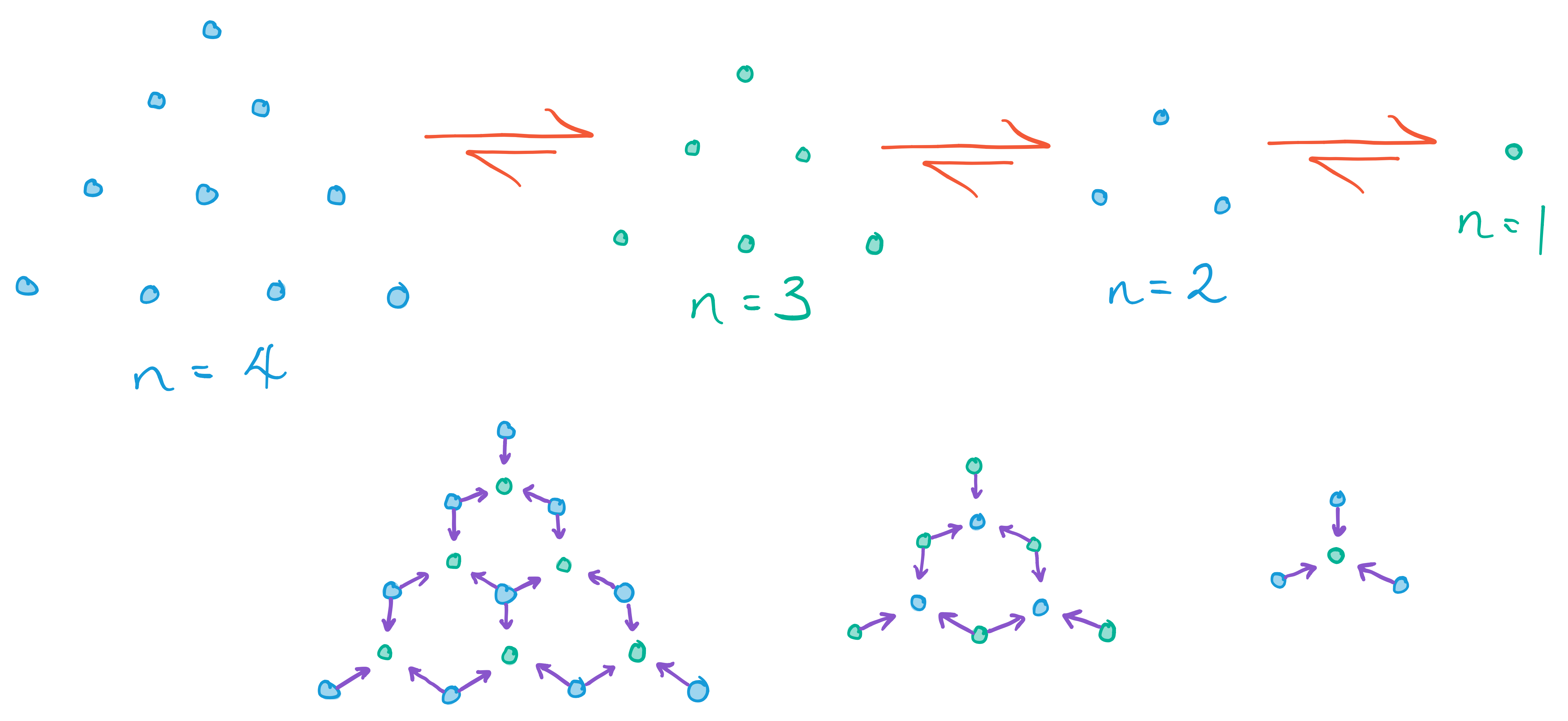
For the upper bound, we first obtain the upper bound on the boundary MFPT as for and for . One needs to be particularly careful for and above as there are different ‘classes’ of boundary nodes: for (as shown in Figure 23), there are ‘vertex’ boundary nodes which have only one forward transition, and ‘edge’ boundary nodes which have two forward transitions, whilst interior nodes have three. More generally, in dimension there are classes of boundary nodes with forward transitions respectively (and interior nodes with forward transitions). The vertex nodes will have the highest MFPTs and correspond precisely to the MFPT, and are therefore what we shall use for MFPT bounds in higher dimensions. The values of can be found by counting transitions, and are , and .
Using these values of the boundary MFPTs and superposition fractions, we can write a recurrence relation for each dimension in ,
with initial conditions
These can finally be solved to yield
and, in the limit of large , these simplify to
In summary, the MFPT penalties for truncated simplices are bounded above and below by
where and . Expressions for higher dimensions can be obtained using the same approach, but the key point to note is that the terms in each order of are present and significant in both the lower and upper bounds and therefore a synchronisation interaction in dimension will be subject to a penalty of order , with the coefficient of the penalty term bounded below by the information loss in the interaction.
11.2.3 Numerical Simulation
In the course of investigating this synchronisation problem, a suite of tools3232 32 https://github.com/hannah-earley/revcomp-synch-rw-mfpt for computing MFPTs was developed, as well as an assortment of other tools3333 33 https://github.com/hannah-earley/revcomp-synch-rw-distribution3434 34 https://github.com/hannah-earley/revcomp-synch-rw-distribution-2. Computing MFPTs in regimes of low bias and unbounded state space is challenging because the probability density tends to diffuse very far from . Attempting to compute it in a deterministic way via the explicit steady state distribution has a high spatial complexity as one must make sure not to prematurely truncate the state space, or else risk underestimating the MFPT. A rough estimate gives a spatial complexity of , and the time complexity will be the product of this spatial complexity and the number of simulation steps to convergence, which will be at least to allow particles from the initial distribution to explore the entire state space.
The alternative is to exploit the Markov property of the system in order to use a stochastic Markov-Chain Monte-Carlo simulation approach, or MCMC. In an MCMC approach we essentially apply the stochastic dynamics of the system to an ensemble of instances of the system. In this case, each instance is a single phase particle, whose coordinate represents the joint state of the underlying mona. Therefore, for an ensemble of size , the spatial complexity will be . Again, the goal is to obtain the steady state distribution of the forced absorbing-boundary system; to ensure conservation of density, we use the teleporting form in which there is a one-to-one correspondence between each particle incident on the absorbing boundary and a particle injected into the initial distribution.
The naive approach is to record the number of time-steps between injection and absorption for each particle. Unfortunately this approach is not robust enough here as the high-diffusion negligible-drift regime leads to substantial variance in the FPT distribution such that a significant proportion of particles in the ensemble will get ‘lost’ in the phase space for an unboundedly long time. Therefore the mean of the particles’ injection-absorption times will typically be divergent, or the program will run indefinitely as it waits for each particle to be absorbed. A possible solution is to exclude particles which have not returned after some predefined number of time-steps, but this will lead to an underestimate of the MFPT.
The correct solution, it transpires, is to instead record the absorption current: that is, within some time-step window , count the number of particles incident on the absorbing boundary in order to obtain an unbiased estimate of the current where is the ensemble size. This process can be repeated as many times as one likes to obtain a series of measurements of the current, from which basic statistics can be used to find an improved estimate of the mean current and its standard error.
There remains, however, a caveat common to all MCMC simulations. Assuming our particles are distributed according to the desired steady state, then their distribution will remain so as they evolve under the stochastic dynamics of the system. The problem is in ensuring that the initial distribution of the system is the steady state, despite not knowing what that is. To address this, one typically initialises the system to an approximation of the steady state and then lets the distribution ‘burn in’ by running the simulation for some number of initial time-steps, after which it is hoped that the approximation will have converged to the steady state. The poorer the quality of the initial approximation to the steady state, the longer this burn-in phase will take. Moreover, the length of the burn-in time can be hard to ascertain and so often one must resort to a heuristic judgement.
Oft forgotten can be the quality of the random number generator used to simulate the stochastic dynamics. In an earlier iteration of this tool, we neglected to consider this and as a result used the standard rand function: a linear congruential generator with period . As the simulation times required to obtain good quality MFPT estimates for many of our parameters exceeded this period, the data obtained was invalid. It can be hard to detect this, and we only realised when a debug trace of the intermediate outputs showed a noticeable and unexpected periodicity. As a result, our MFPT suite now uses the PCG family of PRNGs [pcg] which have an internal state space size and period of whilst also being very fast.
Whilst the dynamics of this system are very simple, some several quadrillion time-steps were required to obtain the data shown in Figure 24 and so a sophisticated toolchain was built around the MCMC routine to improve robustness and automatability. The core program, ./walk, is written in C++ and makes use of OpenMP for parallelisation. Simulating an ensemble of random walkers is an embarrassingly parallel problem, meaning that performance can generally scale linearly with the number of available CPUs due to the minimal amount of inter-thread synchronisation necessary. Unfortunately the GCC and LLVM compilers3535 35 In our experience, LLVM’s optimisation was far better than that of GCC in this case. were not able to fully optimise the inner loop responsible for executing the stochastic dynamics, and so some hand tuning was necessary to improve the assembly output and bring down the iteration time to on the machines used. To ensure resumable operation and cooperation with cluster scheduling systems such as slurm, the program supports checkpointing (both intermittent and in response to trappable signals). The program is also reasonably modular, making it straightforward to adapt to new random walk systems.
To coordinate simulating the large number of parameters across different topologies of networked systems and to minimise need for manual intervention, a batched job runner was developed in the form of a python script. The job runner has three modes of operation; it can take a description of a set of jobs and generate specific instructions for each job, it can connect to a distributed job queue to request and run these jobs, and it can query the status of all the jobs and job runners (optionally sending updates by email at regular intervals). A key feature is that it can analyse the output of ./walk to determine whether the error has converged to a sufficiently small value, whereupon it will move onto the next job. Finally, a number of tools were created to analyse the resulting data, including the ability to infer and inspect the approximate steady state distribution over the phase space.
The results of these simulation tools are shown in Figure 24. As well as serving as a sanity check on the derived MFPT bounds, we were also able to obtain an estimated empirical equation for the true MFPT as
| (4) |
where the term is inspired by the exact MFPT for , given by . In particular these tools were very helpful in getting an intuitive feel for the parametric dependence of the MFPT when analytic approaches seemed unyielding.
11.3 Continuous Phase Spaces
The approach for continuous phase spaces will largely follow that for discrete, except that we shall make use of the Fokker-Planck equation as introduced in Section 10.2. In order to solve for the reflective steady state, we shall use the fact that its current vanishes. Recall that the continuous current is given by where is the phase density, the drift coefficient and the diffusion matrix. When is non-singular, this can be rewritten as where and is defined by . If the current is identically zero, then it immediately follows that the density is given by where is a normalisation constant. This is fairly standard, and a similar result is obtained in Chapter 6 of [risken].
To connect this reflective-boundary distribution with the absorbing-boundary distribution, we must find the absorption current. We assume that our reflective-boundary distribution is approximately equivalent to an absorbing-boundary distribution with forcing applied at the hypersurface, where is a coordinate orthogonal to the hypersurfaces; in the limit this becomes exact, in analogy with the discrete case. The true absorbing-boundary distribution has vanishing density at by definition, and therefore we can recover our desired distribution by introducing an appropriate decay from to . In the limit any higher order polynomial terms in this decay will vanish, and therefore the decay can be assumed linear. The absorption current is then given by
Using the fact that the current is along the direction, we can find the normalisation constant subject to the constraint that the total absorption current is 1 as . Therefore we find that the MFPT from is given by , from which we find the lower bound for the MFPT from arbitrary ,
where is averaged over the given hypersurface and is the area of that hypersurface. We see that the MFPT for general phase space is easier to express in the continuum limit, and in the particular case of linear in , i.e. , this reduces to a Laplace transform:
Truncated Simplices
For the Truncated Simplex example in dimensions, the drift coefficient is constant uniform in the direction and the diffusion matrix is the constant uniform and isotropic . Therefore, and we have from earlier that
Hence, the MFPT lower bound for arbitrary may be obtained thus:
12 Recessive Case
We turn now to the recessive case, for which we shall assume a continuous phase space for simplicity. We shall also restrict our attention to recessive systems whose diffusion matrices are uniform and isotropic, , across and whose drift vectors are constant uniform in ; the condition on in will become apparent later, but for now we shall assume it takes the same value as in . Finally, we adopt an orthogonal coordinate system where is chosen such that . It may appear that indexes the hypersurfaces, but this is in fact not the case; a coordinate transform that would render a hypersurface index would apply a shear and therefore make anisotropic.
MFPT Approach
Unfortunately the reflective steady state approach used for the constrictive case is inapplicable here as the unbounded transverse width of the space means the steady state is everywhere vanishing. Moreover, ignoring the zero normalisation, the uniform initial distribution is undesirable. For the canonical example shown in , initial distributions of interest are typically centered on the line (corresponding to the white dashed line in the Figure). Nonetheless, we can apply3636 36 Our simulation suite is specialised to the case of walks in a single quadrant (with a possibly truncated boundary). Whilst it would not be too difficult to handle more general geometries, this particular three-quadrant example can be easily transformed into a single quadrant walk. First, we identify that the geometry is symmetric in the line and therefore the three quadrants are mapped to one and a half, with a reflective boundary placed at . That is, . Next, we apply a shear to map the region to the top-left quadrant. The transformed transitions turn out to correspond to those of Gessel walks, a summary of which is presented by [bm-gessel] along with an investigation of their generating function. the simulation suite introduced in Section 11.2.3. The results for an initial delta distribution on the line and a distance from are shown in Figure 25 and reveal an empirical MFPT of and therefore a penalty of order .
This penalty would appear to be a significant improvement over that for the constrictive case of . Unfortunately this penalty is invalid because in fact the MFPT is not an appropriate quantity to use here. The reason is that the time quantity we are seeking is where is a hypersurface index, and the use of the MFPT is predicated upon the idea that an initial distribution within has for all positive . It is straightforward to see that this property does not apply in the recessive case: Consider a simplified view of as just the four quadrant domain such that and and with ; the hypersurfaces are given by , i.e. . Now, the evolution of a phase particle may be decomposed into that along the line and perpendicular to this line. Calling these coordinates and respectively, i.e. and , we see that the distribution is given by the product of two Gaussians, with probability density
Now, the expected hypersurface is given by
and therefore an initial distribution will tend to go backwards in -space for a time , retreating as far back as before it begins to advance; at time it returns to its initial position whereupon it begins to make net progress. The consequence is that there is a time penalty for all , and hence the appropriate boundary to consider for the MFPT calculation is given by .
Of course, in the case of constant uniform across we are able to use the far simpler approach of considering the exact probability distribution, as detailed above. We can also extend easily to arbitrary boundary shape. Unfortunately, as mentioned, may well differ between and . For our canonical example in coordinates,
That is, in the drift direction is towards the axis. Recall also that we have ignored the six-quadrant structure, and so there is in a sense a lot more ‘space’ in . Nevertheless, we will be able to obtain lower and upper bounds.
Probability Distribution Approach
Ignoring the caveat about for now, we proceed for a general boundary shape . For the canonical example, . Without loss of generality, we pick and we note that a recessive geometry implies increases monotonically away from . We then have ; decomposing into its even and odd parts, and respectively, we see that whenever the initial distribution is even because the transverse dynamics respect evenness. As we are considering the initial distribution , we discard the odd part of without loss of generality.
If has a power series expansion about , it will take the form . Series representations do not exist for many boundary shape functions of interest however, in particular has no such expansion. Consider instead a smooth function such that ; if exists, it has series expansion and hence will have series expansion . We can then compute as where and , and is the double factorial.
For the case , and we will find a penalty of order as earlier. If instead is quadratic, then and there are two subcases: if then the rate of computation is reduced to within a large vicinity of the synchronisation interaction; if then computation halts or goes backwards, and the synchronisation never3737 37 It is possible to escape if the phase geometry eventually changes to a permissible form, but the penalty will be substantial. occurs. As we are considering systems with arbitrarily low bias, and hence , this effectively means that quadratic boundaries are untenable. For cubic and above, briefly increases before decreasing forever. From these, we can deduce that should ideally be (absolute) linear, though it is admissible to also have a small quadratic component if is bounded from below by .
We now show how to find lower and upper bounds for per our canonical example, that is and . In both regions, the action of the drift vector alone is to increase . The direction of in acts to pull the distribution further away from than would be the case if pointed -wards; therefore, picking constant uniform will retard the process of synchronisation and thereby result in an upper bound. Alternatively we can advance the process by picking a uniform superposition of the two, , letting the extra ‘space’ in the axis apply to too. This extra ‘space’ would appear to complicate matters further, but we can avoid this complication by realising that the action of this -wards drift is simply to increase the value of and therefore it is equivalent to setting . Solving for the bounds finally yields
which for our canonical example reduces to
This shows that the penalty is at least of order and, for small , is as high as . In other words, the penalty is worse than for the constrictive case. Interestingly however, the penalty is almost exactly the same for higher dimensions if the boundary is replaced by a hypersurface of revolution of ; in fact, in dimension we find
but otherwise the form of the synchronisation times remains the same. As a result, using a recessive synchronisation geometry is an alternative way of efficiently synchronising in dimensions and above. Of course, a sequence of constrictive synchronisations will limit the penalty to order and so constrictive synchronisation geometries remain the most effective approach.
13 Constrictive Generating Functions
Finally, we present some limited successes towards generating functions for the MFPT for arbitrary initial distribution. We shall consider the truncated simplex for and , as shown in . To do so, we must construct a function to enumerate all possible walks from each initial position and weight them by their probabilities. A walk starts at some initial position (for convenience we use the upper right quadrant), takes a number of up, down, left and right steps, and terminates at the origin. It is also subject to the constraint that it must not reach the origin until its final step, and if the walker is on a reflective boundary then a forbidden step (left or down, depending on which boundary) is replaced by a null step with the same probability but which leaves its position unchanged.
Constructing a generating function subject to these constraints is easier in reverse. Let the variables of the generating function be , and , such that a term indicates that a walk starting at reaches the origin in steps with probability . As all walks almost surely reach the origin in a finite time, and so if then . To construct such a from walks in reverse, we start from the origin and walk anywhere in the plane for any number of steps. As we shall be handling the origin specially, we start with the last step which must be from either or . The probability that the next step from either of these reaches the origin is , and therefore these two particular walks are given by the initial term . Given a walk of length starting at , we can construct a walk of length by prepending it with each of the four possible steps. Ignoring the boundary conditions, this means we can generate a longer walk as where . Note that corresponds to prepending a downward step with probability , but we increase the power of because the power of is the starting position. If is of the form or , then we replace respectively the steps or with (this is not a typo; to see that is correct it is helpful to work through an example walk). Lastly we must ensure walks avoid the origin, or at least that we ignore those walks which prematurely reach the origin. We do so by ‘trapping’ such walks so that they get stuck there by excluding these walks from the transitions. Assembling these, we obtain the functional equation
| (5) |
which can be written more usefully in the form
| (6) | ||||
where , , , and is known as the kernel.
Orbital Sum Approach
We now apply the orbital sum approach as detailed by [bm-walks]. The group of the kernel is defined to be the set of maps that leave the kernel unchanged, with the group operation taken to be function composition, . For this kernel it is generated by the orthogonal involutions and , and hence is finite with order 4. Explicitly, the elements of the group are . We also define the ‘sign’ of each element, , as and . When finite, this group has the interesting property that the ‘orbital sum’ of a function of just or under this group vanishes, i.e. .
Looking at our functional equation 6, all of the terms on the right hand side are functions of both and . However, by dividing through by we can make two of these terms functions of only one of and . We need to be careful however, as generating functions have ring structure but don’t generally admit an operation corresponding to division. Moreover, we are dividing through by series in negative powers of and , and so we need to consider the Laurent series structure. Specifically our series belong to the ring of formal power series in whose coefficients are Laurent polynomials in and , and the series belongs to the ring of formal power series in whose coefficients are polynomials in and . To perform the division, we observe that the series annihilates under multiplication and therefore is an appropriate multiplicative inverse to use.
Multiplying through then and taking the orbital sum, we find
Recalling that is invariant with respect to the group, we can rewrite as
To proceed, observe that remains part of the ring . Moreover, every term has a positive power in and . Therefore, the orbital sum yields the sum of series in the rings , , and , and so if we extract the positive part consisting of only the terms with positive powers of and , then we can find an expression for
where is the positive part of . There is a limitation here: if can be written as then the orbital sum of the term in this scheme will vanish because is invariant under the group, as is the part. Moreover, any other functions which vanish under the orbital sum will also be excluded from our apparent . This means, for example, that evaluating the above expression for will yield 0 because is in fact .
The MFPT starting from is given by , and its generating function is . It is easy to show, therefore, that and so we find
assuming that has no terms which vanish under the orbital sum. It remains to find , and to determine whether or not has any such terms.
Obstinate Kernel Method
Another approach is given by the obstinate kernel method, wherein we exploit roots of the kernel. A pair of such roots is given by where , , and is a symmetric function of and . It will be helpful to note the elementary symmetric polynomials of as and . Only one of these roots, , is a power series in ; the other includes a term in , and so we shall substitute into the functional equation 6 to get
To solve for , and thence , we eliminate by making use of the kernel’s group; in particular applying yields a second equation in ,
from which we find
with . Extracting the positive part then gives
From , can be obtained and thereby and . Alternatively, the MFPTs for arbitrary positions can be computed using the recurrence relations and the boundary MFPTs . In order to do so, we shall need to obtain an expression for . Letting , we see that and we compute using Equation 5 to find . Therefore we can obtain an expression for ,
Using the symmetric variable helps to evaluate the positive parts of the antisymmetric series , but we were unable to proceed beyond this point.
14 Applicability to Other Architectures
Finally, we comment on the applicability of these results to non-Brownian reversible computers in the limit of vanishing free energy density. The concepts of mona and synchronisation phase space can be readily extended to other models of communicating reversible computer, but the time evolution of the phase space distribution may differ. In many architectures, the probability of a backward transition approaches 0. Nevertheless, it is still possible for the joint distribution of mona in phase space to expand over time. In particular, if the eigenstates of the Hamiltonian change over time due to thermal fluctuations, then the rate of computation at different independent loci will fluctuate and so synchronisation will be lost. Moreover, universal phenomena such as the Heisenberg uncertainty principle and general relativistic time dilation effects suggest that even a system at absolute zero would experience desynchronisation.
An important assumption in the above, and indeed this chapter, was that the mona evolve independently except during synchronisation events. As argued by [frank-coupled-sync] in a thought experiment, however, it is possible to couple the mona in a system with a potential that increases with increasing desynchronisation. In particular he imagined a lattice of clockwork computational units driven by a series of motors, with adjacent axles connected by bicycle chains. At low speeds , the power supplied to counter frictional losses in the system would scale with where is the number of mona, which recovers the scaling law. Any tension due to desynchronisation between adjacent mona would not substantially increase this power requirement, not least because adjacent axles experience equal and opposite tensions. Therefore the introduction of such potentials may be used to constrain the size of the joint phase distribution of adjacent mona; that is, mona remain locally in approximate synchronisation. Globally, remote mona may accumulate more significant desynchronisation, scaling with where is linear dimension of the system and the temperature, but this would not pose any problems to long-distance communication as long as message packets remain in local synchronisation at all points along their routes.
As a corollary, we extend Frank’s thought experiment to a general conjecture about which classes of reversible computer are and are not subject to a synchronisation penalty:
Conjecture 14.1 (Inter-monon synchronisation potentials are a necessary condition for cheap communication).
By the above arguments, we conjecture that the joint phase space of independently evolving mona cannot remain localised, and hence that the synchronisation penalties derived in this chapter apply for all such reversible computer architectures. Conversely, mona whose evolution is coupled by a potential that increases with increasing desynchronisation will remain localised, and therefore can in principle pass through synchronisation windows with arbitrarily low penalty. If the distribution can be constrained to be compact, then the penalty may be eliminated.
However, this is predicated on communicating mona being carefully programmed. Communicating mona must anticipate each other’s computational states, such that they are both simultaneously (up to the width of the synchronisation window) receptive to communication. If a monon attempts to send information to another monon that is not expecting to receive such information, then this will incur an entropic synchronisation penalty by the mechanisms discussed in this chapter. Alternatively, a radically different approach to eliminating communication penalties is given by fully serial architectures, such as is theoretically permitted by a Quantum Zeno architecture (Section 2).
An interesting example of an architecture where careful ordering is intrinsic to the computation itself is the BARC3838 38 BARC was historically referred to as ABRC, the Asynchronous Ballistic Reversible Computing model. (Ballistic Asynchronous Reversible Computing) model of [frank-barc]. BARC systems consist of devices with an internal state, and wires between them along which pulses can travel. Devices are designed to interact with at most one pulse at a given time, the effect of which may be to change the device’s internal state and to re-emit the pulse along a different wire. As the order of signals is important to the computation, any well-designed BARC computer will satisfy the synchronisation simultaneity condition. In this case, the synchronisation window depends on pulse spacing. Additionally it is an architecture without backwards transitions. However, the architecture—as presented—does not couple pulses to each other with a synchronisation potential, and so it is subject to the conclusions of this chapter as the ordering between free signals is subject to change. Nevertheless, this desynchronisation can be kept impressively minimal through the high efficiencies and engineering tolerances afforded by superconducting circuits (see [frank-barc-fluxon] for progress towards a Single Flux Quanta implementation of the BARC model).
Petri Nets
Another model of asynchronous concurrency that is quite popular is that of Petri Nets (see [petri] for a review). A Petri Net is a weighted directed graph with two types of nodes, ‘places’ and ‘transitions’. A place contains tokens, and the configuration of tokens in all places—a ‘marking’—represents the state of the system. Tokens can be consumed, generated, and moved by the activation of a transition. A transition node consumes some tokens from each place connected to it by an incoming edge, and deposits some tokens to each place connected by an outgoing edge. Edges may only be drawn between a transition and a place, and the weight of the edge dictates the number of tokens involved in the transition. A transition may only activate if there are enough input tokens.
Whilst a Petri Net is not necessarily reversible in the sense of having a corresponding inverse transition for every transition, it is always possible to construct an ‘inverse Petri Net’ by inverting each edge’s direction. From this perspective, a Petri Net along with its sequence of transitions form a logically reversible system. It is not immediately obvious where entropy costs manifest in a Petri Net, and so it may appear that they offer a route to avoid the conclusions of this chapter. In order to accommodate entropy costs, the sequence of transitions needs closer attention. Without loss of generality, assume discrete time where at each time step a single3939 39 Multiple transitions can occur simultaneously only if they do not share any places, but then they can always be assigned an arbitrary order and treated as sequential. transition is attempted. If every transition is always successful, then there is no entropy increase. If, however, a transition may fail, then reversibility requires us to record a binary outcome of success or failure. That is, the input is a stream of symbols—each corresponding to a particular transition—and the output is a stream of symbol-outcome pairs. This is where entropy may increase, and is another example of a breakdown of simultaneity in synchronisation. Moreover, such a system—in which the transition order is sequential—does not allow for separate independent entities, let alone spatial structure. Therefore the notion of synchronisation/communication is not particularly relevant. To accommodate this, multiple transition streams can be introduced. For avoidance of conflict, the streams must satisfy the constraint that no two transitions sharing a place fire at the same time. Now the issues of synchronicity of signals and events become manifest: if these transition streams can be coupled to each other to maintain some local synchronisation then low cost communication can be supported, otherwise there will be a synchronisation penalty. Therefore, whilst Petri Nets are a convenient framework for modelling asynchronous systems, they are not particularly convenient for modelling the possibility of desynchronisation and the resultant resynchronisation entropy costs.
15 Conclusion
The primary result of this chapter is that communication between distinct reversible computers in a Brownian system (and arguably any reversible architecture whose mona evolve independently) with a limiting supply of free energy is very expensive in comparison to independent computation. A single computational step takes time for gross computational rate and bias , where is the rate of supply of free energy, is the number of mona, is Boltzmann’s constant, and is the system’s average temperature. In contrast, an interaction event such as communication takes at least a time . As the bias scales as for a system of convex bounding surface area , internal volume and radius , communication will tend to ‘freeze’ out as the system gets bigger. This cost is unavoidable as it is due to the implicit erasure of information involved in synchronising divergent computational states; however, if synchronisation is rare then the temporal cost can be reduced. Suppose that the average proportion of mona wishing to communicate at a given time is , then the free energy can be divided into two supplies: and for independent computation and synchronisation events respectively, as intimated in Section 7. A separate set of bias klona can then be introduced for the synchronising mona,
In order for the synchronisation to be viable we therefore require and hence find
If we want to maintain our asymptotic independent computation rate of , then we will have and , giving . That is, the number of synchronising mona can be as high as . In fact, this subpopulation of mona are also permitted to perform arbitrary operations subject to entropic costs, with the proviso that their individual net transition rates will be . The consequence is that, for a very large reversible Brownian computer, any parallel computation should be structured to minimise the need to synchronise the joint state of the system. Equivalently, the proportion of computational steps that are permitted to synchronise is . If one wishes to increase the proportion of synchronising mona, then the total computational rate must necessarily be reduced or an architecture satisfying 14.1 must be employed.
Impact on Algorithms
The consequence of this ‘freezing’ out of synchronisation is that the most natural computational problems for these computers are those which are ‘embarrasingly parallel’. An embarrasingly parallel problem is one which can be easily divided into many tasks with very infrequent synchronisations between them. Some examples of such problems are Monte Carlo algorithms, brute force searches, and ray tracing. In contrast, highly serial problems, or parallel problems involving significant synchronisation, are not well accommodated. Serial programs suffer because the rate of computation by individual mona is asymptotically vanishing. Highly synchronous parallel programs suffer because of the time penalty for synchronisations. In limiting cases where no parallelisation is possible or where synchronisation cannot be made arbitrarily infrequent, the rate of these computations will fall to as with irreversible computers. Nevertheless, as discussed in Section 7, hybrid computational systems supporting both high-bias and low-bias subsystems can be constructed. Therefore serial/highly synchronous problems can be executed on a thin outer shell of the computer, and embarrassingly parallel problems can make use of the inner bulk of the computational matter.
A common example of highly synchronous parallel problems is that of simulating systems involving local interactions on a lattice, such as cellular automata, Ising models, and molecular dynamics simulations. Indeed, in [frank-thesis] (Section 6.3.2.1), he examines local computation by a three dimensional array of computing elements. For the class of non-Brownian computers under consideration, he finds an asymptotic benefit for reversible architectures over irreversible architectures. Unfortunately the results of this chapter show that problems like these are not well-supported by Brownian architectures, and so this asymptotic benefit is not seen in this case. However, the thought experiment of [frank-coupled-sync] and 14.1 do support the realisation of such asymptotic benefit in architectures in which the computing elements are appropriately coupled.
This chapter concludes our analysis of the limits the laws of physics place on the sustained performance of reversible computers. id1 concerned aggregate performance in terms of computational operations per unit time, but neglected to consider interactions among computational sub-units or between computational sub-units and shared resources such as memory or chemical species. id1 extended the analysis to consider the former set of interactions. In this chapter we extend the analysis to consider the latter set, which in general will be governed by the laws of thermodynamics and statistical mechanics. When the free energy available to the computational subunits is limiting, this becomes a challenging endeavour as perturbations to these subsystems may have a corresponding entropy cost for which our available free energy is insufficient.
In the first half we pay particular attention to resource distribution: Our Brownian computational subunits—themselves being small and particulate—will likely lack adequate internal memory for many programs of interest; as such, it can be expected that a realistic Brownian system will make heavy use of a shared pool of memory resources that can be dynamically distributed amongst the computational subunits according to their need. It is found that most schemes imaginable fail to function effectively in the limit of vanishing ‘computational bias’ , which measures the net fraction of transitions which are successful and which falls as the system grows in size.
Driving thermodynamically unfavourable reactions, such as resource distribution, is a very general problem for such systems and can be solved by supplying a sufficient excess of free energy. In order to make these interactions viable, we propose an abstract chemical scheme to dynamically infer how much free energy is needed, and to supply it by accumulating just enough from the (weak) ambient free energy. The scheme takes any reaction, arbitrarily far from equilibrium, and sequesters some of the reactants and products such that the extant reactants and products are in equilibrium. The scheme rapidly adjusts to changes in the equilibrium position, and makes use of molecular computation for its inference algorithm. Unfortunately there is a cost in applying this scheme: the reaction is slowed by a factor inversely proportional to the ‘computational bias’, (the net proportion of computational transitions that are successful). In fact, this overhead is comparable to that found for synchronisation interactions in id1.
Chapter Performance Trade-offs for Reversible Computers Sharing Resources

16 Introduction
This is the final chapter investigating the influence of the laws of physics on computation, particularly as they apply to large reversible Brownian computers (see 9.2). As discussed in id1, the net computational rate (in terms of primitive computational operations per unit time) studied in id1 is not the only performance metric of interest. Therefore, in id1 we evaluated computational performance of reversible Brownian computers (and argued for the applicability of the results to other reversible computers whose computational units evolve independently) whose individual computational components were permitted to interact with one another, i.e. to communicate and to perform concurrent/parallel computation. A key property of these interactions is that computational ‘particles’ can be uniquely referenced, and therefore the traditional thermodynamic principles that apply to chemical systems were inapplicable. In this chapter, we now consider the interface between traditional chemical species, of which there may be a variable number of identical units or particles, and the computational particles. See Figure 26 for an illustration. For convenience, we shall refer to these as klona and mona respectively, following the formulation introduced in 9.1. Recalling the definitions, we call particles which are uniquely distinguishable or addressable mona (sg. monon), after the Greek for unique, μοναδικός. Similarly, we call indistinct particles belonging to a species klona (sg. klonon). Klona may be likened to traditional chemical species such as glucose and ATP. Mona are less obvious; an example would be a solution containing a concentration of random nucleic acids of length 80 nucleotides.
Interactions between mona and klona are of great practical importance for Brownian computers; whilst mona by themselves may be capable of arbitrary computation, this computation only becomes useful when used to actuate some other system or when it otherwise produces some observable output. Examples may include the activation of a fluorophore upon reaching some logical condition, or directing the translation of a particular messenger RNA into a protein. Moreover, interaction with klona may be essential for computation: general computation requires access to an unbounded amount of memory, but by their very nature mona are limited in size and thus memory. Therefore it is important for mona to be able to recruit more memory as required, and release it for use by other mona when the need passes. Resources other than memory may also be considered, such as structural monomers for use in constructing and deconstructing molecular machines or computers.
In this chapter we shall be most interested in the case of resource distribution, and will consider various such schemes in Section 17. One approach is a centralised store which mona can access, either by travelling there themselves or by sending a ‘courier’ monon on their behalf to fetch and retrieve (or carry and return) a resource. This approach is undesirable. If the couriers float freely in solution, then reaching the central store and returning will both take a time ; if on the other hand we introduce a lattice as in id1, then the average distance will be proportional to the radius and, given , the average time will be . As the time for a single net computational step is , both of these are untenable. Instead we shall seek a decentralised approach by making use of klona; intuitively it must become harder to access a resource as its scarcity increases, but we would like the timescale to do so to not be substantially more costly than where is the available concentration of the resource.
We will unfortunately find that the reactions involved in all possible schemes are unfavourable except in a very limited range of resource availability. In Section 18 we shall return to considering general mona-klona interactions, and demonstrate how mona can dynamically drive any unfavourable reaction with klona by inferring the number of bias tokens required to balance the entropic cost of the reaction. Alas, there will turn out to be an overhead in achieving this even in the case when the driven reaction is at equilibrium and hence cost-free.
17 Resource Distribution Schemes
A resource distribution scheme for a resource is a set of klona from which can be extracted and into which it can be deposited. Formally, resources are conserved discrete quantities analogous to charges in physics. Letting the set of resource species be indexed by and the set of resource klona by , then to each klonon is associated a resource charge : a vector over the field of naturals and indexed by the resource species. In any reaction, the net resource charge must be conserved; for example, for the reaction involving the transition of a monon between states and and the interaction of said monon with resource klona according to the stoichiometries , this conservation law can be expressed as .
Free Klona
The simplest possible scheme is that in which the resource is freely present in solution, as shown in . That is, a system with , and . This system will be a viable resource pool so long as the free energy change involved in both extraction and deposition of is less than the available computational free energy, . Note that our notion of ‘free energy’ uses a different convention than is normally taken, namely we are giving the change in information entropy of the universe , whereas normally the free energy change is expressed as . The free energy change vanishes when the system is in equilibrium, which for an ideal gas can be calculated (via the Sackur-Tetrode equation) to occur at a concentration
whereh_PmXuXμ_Xμ_X= log [X]γ X [X]γ X — (eq.) γ_XXXQX[X]QδQQ ∂ log γ ∂ log Q =-1≪1X
Bounded Carriers
Perhaps the primary issue with free klona is that there is a change in particle number, implying a substantial entropy change when resources are traded with the pool. A possible improvement is suggested in ensuring total particle number remains constant by binding the resource to carrier klona, as shown in . This may manifest, for example, as with and . More generally, we have polymeric klona with for some integer . Once again, we shall consider a perturbation to the equilibrium distribution of the pool; it will be convenient to introduce a partition function where the thermodynamic variable correlates with the amount of resource stored by the pool. The partition function will take the form where contains all the thermodynamically pertinent information about klona, such as its energy and internal degrees of freedom. In fact, we will take as any -dependence of the would only serve to reduce the effective value of by narrowing the distribution4040 40 Assuming that the equilibrium distribution is unimodal, this corresponds to a reduction in variance. If the distribution is multimodal then instead there is a reduced ‘local’ variance about each mode..
The free energy change for a reaction is given by the logarithm of the ratios of reaction rates (see, e.g., Section 4 for a derivation). Therefore in this case it is given by , and so at equilibrium (when ) we find . For a perturbation from equilibrium, this reduces (exactly) to . Now, the average -charge of each klonon is given by , and the charge density by . The proportional resource accessibility is then given by
using and . This suggests taking to ensure full resource availability. Unfortunately, doing so would mean the total system charge scales as which clearly cannot be sustained in the limit of large systems. One potential resolution is to reduce the carrier concentration to and then take so that the total charge scales with ; whilst this would slow down resource reactions commensurately, mona could use this additional time to accumulate tokens in order to raise their free energy budget to , thereby obtaining a resource accessibility of at a time penalty of .
Unbounded Carriers
It is also possible to consider polymeric klona of unbounded size, i.e. the limit , in which case the partition function is given by . It should be noted that in this limit there is no equilibrium distribution of the resources, as diverges as . In fact, distributions only exist for whilst the free energy constraint bounds it from above and hence . This range corresponds to and therefore a total enclosed charge ; for lower densities, the only favourable reaction is resource deposition. Therefore, whilst conceptually simpler, unbounded carriers are to be avoided.
Isobaric Compartments
The problem inherent to seemingly all schemes is that a resource reaction must necessarily reduce the quantity of reactants and increase the quantity of products, and this will in turn bias the resource reactions in the opposite direction per Le Chatelier’s principle. As our last attempt to circumvent these issues, we introduce a scheme exploiting varying partial volumes in order to maintain equal concentrations of reactants and products. This ‘Isobaric Compartment’ scheme is illustrated in and consists of dividing the system into two compartments by means of a massless and infinitely flexible membrane, impermeable to the carrier species and . Referring to the two compartments by and , we then establish the invariants that only contains and only contains . A monon wishing to exchange resources with the pool must first bind to the membrane, and then to maintain the invariant it will translocate the carrier species between the two compartments. At equilibrium, the concentrations of carrier species in each compartment must be equal and thus it would appear that we have been successful in eliminating the free energy cost for this mona-klona interaction.
Unfortunately, whilst the carrier species concentrations are equal, concentration is not the correct quantity for determining the reaction rates and thence the free energy difference. From a collision theory perspective, the reaction rates are given by the frequency with which mona and klona collide (in the correct orientation and conformation). Consider the case where all but one carrier reside within : if the total number of carriers is then the mean volume of will be and the mean concentration . This would suggest that a monon bound to the interfacial membrane will encounter the klonon as often as it does an klonon, but this clearly cannot be the case. If we imagine the klonon as residing within a small bubble of volume , then whilst its local concentration is indeed the same as for the klona, the bubble itself is free to migrate anywhere along the membrane. Consequently, in a system in which particles can bind to the boundary of the system in addition to exploring their volume, the effective concentration becomes where is the effective ‘volume’ of the boundary (proportional to its area) and is the enclosed conventional volume. For our isobaric system, (and similarly for ) where the constant is the volume available to each particle. We can therefore write where is the ‘true’ concentration; redefining terms, we let .
The system can be generalised to carriers for by letting the membrane be semi-permeable to , as these klona can participate as both reactants and products in either reaction. We can then write for the partition function of and similarly for . The effective concentrations of in each compartment must be equal for , i.e. . As this must apply for each , must be constant with respect to and therefore . Moreover, . Equilibrium occurs once again for with corresponding ‘true’ concentrations . The free energy difference is then given by
Finally, the resource charge is and hence the proportional availability is given by
recallingthatγ≡1/[X]n∼1/bα∼bn=1αα∼b^2Aα∼1∼b^-1α∼b∼V^5/6∼b^-2
18 Driving Unfavourable Reactions
We conjecture that the results in the previous section are general; that is, no resource scheme can achieve better resource availability under the same constraints. In order to make use of a greater proportion of the resource pool, more free energy must be supplied and, ideally, the amount of free energy supplied should be the minimum necessary to avoid wasting the supply of negentropy. As alluded to in the introduction, we shall now consider general mona-klona interactions of arbitrary free energy cost.
Reactions of Known or Bounded Cost
Consider an arbitrary reaction with forward reaction rate and backward rate . Recalling that the free energy change for the forward reaction is given by , it can be seen that computational bias tokens are needed to drive the reaction forward in the case ; similarly, if then tokens are needed to drive the reaction backward. In addition, if we wish to couple such an unfavourable reaction to our computational mona then we should ensure by some means that the reaction does not occur in uncoupled isolation, such as raising the activation energy of the reaction or by employing a reaction mechanism that requires interaction with the mona. This kind of coupling abounds in nature, wherein a variety of bias systems are exploited. In fact, the bias system is itself generated from a number of other bias sources. One particular example involves the conversion of the free energy of a transmembrane proton gradient for which ; the molecular machine responsible for this coupling, ATP synthase, is a molecular motor which translocates 11 protons4141 41 The exact number varies between species, and even between different organelles of the same species, but is typically between 10 and 14. across the membrane per revolution, in the process converting 3 molecules of to , an entropically unfavourable process.
When is known and fixed (or, at least, bounded from above) an optimal approach is provided by the simple scheme that performs transitions between each unfavourable reaction. Indexing the mona states, , modulo , the scheme can be written thus
The reactions between and serve to increase the ratio such that it counteracts the ratio . To solve for the steady state dynamics of this system, we write the currents
andusethefactthat,atsteadystate,thecurrentsmustbeequal.Moreover,thecurrentwillcorrespondtothenetrateatwhichthetargetreactionisdriven,andthereforewecanfindtheoptimalchoiceofn¿—Δh/2arctanhb—nnand . This yields , precisely the threshold value of . The attentive reader may point out that this value of is not necessarily integral, and therefore a cyclic chain of length may not exist; this is true, but we shall be seeking larger values of to increase the rate of the reaction and for which picking the nearest integral value shall be acceptable. Alternatively, one could consider the superposition of two such chains for and in the appropriate proportions.
To solve for non-vanishing current, we perform two telescopic sums
wheret≡ p q S(↦)[][]γ≡β/αn=2n_0 + n_0=—Δh—/2arctanhbnS →[M]min(2b^2λ α β , 2bα)nnbλ
Reactions of Unknown or Unbounded Cost
The preceding scheme suffers from a number of shortcomings due to the fact that is fixed; when is lower than that designed for, the system expends more bias tokens than necessary, whereas when it is greater the system will stall. Moreover the system is asymmetric with respect to direction of the driven reaction: if then the forward reaction should be driven with tokens whilst the reverse reaction needs no additional bias, but this complicates the act of running a subroutine in reverse as each bias chain for the forward reaction must be removed, and a bias chain must be introduced for each instance of the reverse reaction. This is further complicated if the intermediate transitions along the chain perform useful computation. Whilst these problems are not insurmountable, it is possible to solve them all with a revised scheme in which is permitted to vary.
A scheme with variable is incompatible with the specific implementation of that for fixed , and so we first migrate the mona chains into a distinct system of klona consisting of the species and subject to reactions , with steady state . To demonstrate practicability, an abstract molecular realisation is provided in Section 19. The idea is to sequester some of the reactants and products in an inactive state, with those remaining in an active state being at equilibrium (for an isenthalpic reaction, this manifests as equal concentrations). Representing the reactants by and the products by , this effective sequestration behaviour is achieved by the reaction with . For fixed , this scheme already solves all the aforementioned problems as the complexed system is an equilibrated abstraction over the underlying reaction, and hence can be coupled directly to the computational mona system.
In the course of system operation, the value of will almost certainly vary. Introducing the sequestration klona for all values of , and letting and , we see that the desired equilibrium condition is given by . Therefore, if the values of and deviate from equilibrium then we should counteract this deviation by perturbing the -distribution of the sequestration klona. Ideal kinetics are attained if this -distribution converges to exponentially fast, i.e. . This target kinetics arises because and , hence increasing increases . A first attempt at implementation might be given by , but this doesn’t quite replicate the desired kinetics. Instead we separate the concerns of the computational bias and the reaction coupling thus:
| (7) |
Assuming that at steady state , the coupled reaction then replicates the kinetics . For symmetry, we have introduced two intermediate mona with their inter-monon transitions used for coupling to the computational bias. In order to ensure that only a single token’s worth of bias is consumed in the reaction, we also introduce two leak reactions such that the total free energy change is precisely that for a single token: .
To verify that this system has the desired properties, we now solve for the steady state distribution. Employing detailed balance, we find for each that
wherewehaveusedtheintra-X[X^(n)_k]/[X^(n)_0]=( p q )^knn_0β’=α’{X:k}t= p q t^nt^- 1 2 (n+ 1 2 -n_0)^2+ 1 2 ( 1 2 -n_0)^2=t^- 1 2 (n- 1 2 -n_0)^2+ 1 2 ( 1 2 +n_0)^2n_0n_0=0—n_0—≫1[X]= b 1+b β’=α’= αb 1+b ∑_n∈ℤt^ 1 8 - 1 2 (n- 1 2 )^22∫_0^∞t^- 1 2 (s+ 1 2 )^2 d s 2∫_0^∞t^- 1 2 (s- 1 2 )^2 d s α’=α πb +n_0≫1β≫αn¿0α’2bα+ β≫α2bβ+ α≫βBβ¿αα’=β’=α( πb ,2b)∝b∼b^-3/2∼b^-2
19 Molecular Counter Implementation
Here we present example implementations of the counter klona used in Section 18. These implementations are abstract, but point towards a viable molecular realisation.
Unary Representation
(intra–bias) M+A: :B + M (pos–step) M+A: :B + M (pos–base) M+A: :B + M (neg–base) M+A: :B + M (neg–step)
Thesimplestimplementationofcountersisgivenbyrepresentingnumbersinunary,i.e. aPeanoaxiomaticapproach.Foranaturalintegern∈ℕn
0≤k≤n
n+1nk
n=k=0
n=-4,0,4knn = ⟦
⟧
Binary Representation
Whilst particularly simple, the unary representation is very space inefficient; worse, incrementing and decrementing , for the purpose of modulating access to a sparse resource/disequilibrium reaction, will itself require interaction with a resource pool in order to acquire and release monomers. Fortunately an exponentially more compact representation exists in the form of positional notations such as binary, with spatial complexity logarithmic in and hence needing far fewer interactions with its respective monomer pool.
Unlike with the unary case, we cannot exploit the structure of the representation of to represent . Instead we shall need to store both explicitly. We will also require the ability to recognise the states and , both for determining whether the coupled reaction should proceed and for ensuring the reactions that generate the intra- distribution do not produce illegal values of . These two states correspond respectively to all the digits of being or being identical to those of . Since , its minimal representation will be no larger than that of and hence a convenient structure for encoding the pair with the ability to easily check the condition is given by a ‘zipped’ double-stranded polymer which we denote by