Singular Bifurcations : a Regularization Theory
Abstract
Several nonlinear and nonequilibrium driven as well as active systems (e.g. microswimmers) show bifurcations from one state to another (for example a transition from a non motile to motile state for microswimmers) when some control parameter reaches a critical value. Bifurcation analysis relies either on a regular perturbative expansion close to the critical point, or on a direct numerical simulation. While many systems exhibit a regular bifurcation such as a pitchfork one, other systems undergo a singular bifurcation not falling in the classical nomenclature, in that the bifurcation normal form is not analytic. We present a swimmer model which offers an exact solution showing a singular normal form, and serves as a guide for the general theory. We provide an adequate general regularization theory that allows us to handle properly the limit of singular bifurcations, and provide several explicit examples of normal forms of singular bifurcations. This study fills a longstanding gap in bifurcations theory.
Introduction.—
Nonequilirium driven systems constitute a large branch of science which has been the subject of active research in the last decades Cross and Hohenberg 1993; Hoyle 2010; Misbah 2017; Cross and Greenside 2012. Typical examples are Bénard convection Goluskin 2015, Turing patterns Turing 1951; Bourgine and Lesne 2011; Misbah 2017, crystal growth Kassner 1996; Saito 1996; Misbah et al. 2010 and so on. By varying a control parameter (e.g. Rayleigh number in convection) the system exhibits a bifurcation from one state (e.g. quiescent fluid) into a new state (the fluid shows convection rolls) when a control parameter reaches a critical value. If designates the distance of the control parameter from the bifurcation point, the amplitude of the field of interest, say convection amplitude , behaves as , known as a pitchfork (classical) bifurcation. In other situations, like driven fluids in a pipe, a transition from a laminar to a non-laminar (turbument) flow takes place beyond a critical Reynolds number in the form of a saddle-node bifurcation Hof et al. 2004. This behavior is also generic for many pattern-forming systemsCross and Hohenberg 1993; Hoyle 2010; Misbah 2017; Cross and Greenside 2012. The dynamics of the amplitude (known as normal form) of these two bifurcations (pitchfork and saddle-node) read respectively
| (1) |
where dot designates time derivative. Other types of bifurcations are also common, such as transcritical, subcriticalCross and Hohenberg 1993; Hoyle 2010; Misbah 2017; Cross and Greenside 2012 and so on. A hallmark of classical bifurcations theory is the regular (analytic) expansion in powers of in Eq.(1). The same holds also in catastrophe theory à la René Thom Thom 2018.
More recently, active matter, a subject of great topicality, has revealed several bifurcations from a non-motile state to a motile one when activity reaches a critical value Izri et al. 2014; Michelin et al. 2013; Rednikov et al. 1994; Jin et al. 2017; Hu et al. 2019; Morozov and Michelin 2019a; Izzet et al. 2020; Hokmabad et al. 2021; Chen et al. 2021. In its simplest version this consists of a particle emitting/absorbing a solute which diffuses and is advected in the suspending fluid. If the emission/absorption rate exceeds a critical value the particle transits from a non-motile to a motile state. The amplitude of the swimming velocity is found to behave (for infinite system size) Rednikov et al. 1994; Morozov and Michelin 2019b; Saha et al. 2021 as (or , ). This is a singular bifurcation behavior as encoded in . In a marked contrast with the classical picture represented by (1) the corresponding normal form reads
| (2) |
This means that the regular amplitude expansion ceases to be valid, as manifested by the non analytical term . Numerical simulations Hu et al. 2019 of this system are, in contrast, consistent with a classical pitchfork bifurcation, . We will see that this is due to finite size in numerical simulations.
Examples of singular nature have been also encountered in crystal growth. It has been shown that the usual perturbative scheme in terms of the crystal surface deformation amplitude is not legitimate Pierre-Louis et al. 1998. Besides these examples, the emergence of singular bifurcations is likely to be abundant, and has been probably overlooked in many numerical simulations (see also conclusion). The purpose of this Letter is to fill this gap.We will show how to handle singular bifurcations from the usual commonly used regular perturbative scheme. We will first illustrate the theory on an explicit example of microswimmer for which an exact analytical solution is obtained. We then present a systematic method on how to properly treat singular bifurcations.
Theory—
It is instructive to begin with an explicit model revealing a singular bifurcation. We first introduce the full model, before considering a simplified version which can be handled fully analytically. The model consists Michelin et al. 2013 of a rigid particle (taken to be a sphere with radius ), which emits/absorbs a solute that diffuses and is advected by the flow. The advection-diffusion equations read as
| (3) |
where is the solute concentration, is the diffusion constant, and are the velocity and pressure fields, obeying Stokes equations. The associated boundary conditions of surface activity and the swimming speed (which will be taken to be along the -direction) are
| (4) |
with , where is the azimuthal angle in spherical coordinates, is the particle radius is the emission rate (: emission, : adsorption), is a mobility factor (which can be either positive or negative); see Michelin et al. 2013 for more details. This model has been studied numerically Michelin et al. 2013; Morozov and Michelin 2019a; Hu et al. 2019, coming to the conclusion that for (with ) sufficiently small the only solution is the non-moving state of the particle, with a concentration field which is symmetric around the particle. When exceeds a critical value it is shown that the concentration field loses its spherical symmetry and a concentration comet develops, resulting in a motion of the particle with a constant velocity . It is found numerically Hu et al. 2019 that is well represented by , where is the critical value of at which the transition from a non motile to a motile state occurs. The determination of the critical condition has also been analyzed by linear stability analysis Michelin et al. 2013; Morozov and Michelin 2019a; Hu et al. 2019. Analytical asymptotic perturbative studiesRednikov et al. 1994; Morozov and Michelin 2019b; Saha et al. 2021 (for an infinite system size) revealed that the velocity of the swimmer follows in fact the following singular behavior .
Exactly solvable model–
The main simplification adopted here is to disregard the fluid, in that the variable is ignored in what follows. A justification of this is the fact that the singular behavior is associated with the concentration field at long distanceRednikov et al. 1994; Morozov and Michelin 2019b; Saha et al. 2021, while the velocity field vanishes at infinite distance from the swimmer. We consider a particle moving at constant speed . A further simplification is that we assume that the particle size is small in comparison to length scales of interest. The only length scale is given by , so our assumption corresponds to assuming . Under this assumption the particle can be taken as a quasi-material point. With these assumptions the corresponding simplified model reads (in the laboratory frame )
| (5) |
where is the emission rate (related to , by )
Using the diffusion propagator the solution is given by
| (6) |
Expression (S22) can be integrated to yield
| (7) |
with (the coordinate in the frame attached to the particle). Along , it is clear that the concentration decays exponentially with distance ahead of the particle, while it decays only algebraically at the rear ( has front-back symmetry). Indeed, the emitted solute is advected (by swimming speed) backwards, enriching the rear zone, whereas ahead of the particle only diffusion can be effective.
Using (4), only the first spherical harmonics enters the expression of velocity, and we obtain , being the first harmonic amplitude, obtained by projection of (8) on that harmonic, so that the velocity satisfies
| (8) |
Expanding for small we obtain
| (9) |
where , and , is the critical Péclet number. In the full model Michelin et al. 2013. Including hydrodynamics close to particle surface we can capture analytically this result SM. The result (9) has been also obtained thanks to a singular perturbative scheme Rednikov et al. 1994; Morozov and Michelin 2019b; Saha et al. 2021. We see from (9) that always exists. When , there exists another solution given by
| (10) |
Expression (10) corresponds to a pitchfork bifurcation (and not trancritical Morozov and Michelin 2019b) where the solution becomes unstable in favor of two symmetric solutions, . This is, however, an atypical behavior of a pitchfork solution, and is traced back to the infinite system size (as seen below). We refer to this bifurcation as singular pitchfork bifurcation. The term ’singular’ refers to the non analytic nature .
Finite size regularizes the bifurcation and turns the singular bifurcation into a classical pitchfork bifurcation (see SM). Another way to regularize the model is via a consupmtion of solute in the bulk. In that case we modify Eq.(5) by adding on the left hide side, where is the consumption rate. We have in mind the possibility that the emitted solute reacts in the bulk and is consumed by another reaction, giving rise to some secondary product. The solution for becomes
| (11) |
with . The equation for becomes
| (12) |
For we recover the singular bifurcation solution, and for we obtain a regular pitchfork bifurcation. Expansion for small provides
| (13) |
Besides the trivial solution , we have which is a classical pitchfork bifurcation, with . Consumption has turned the singular bifurcation into a regular bifurcation.
Regularization theory–
The expression of type (13) is the one that one would usually obtain by an analytical expansion in in the absence of an exact solution. By trying to compare it to the exact solution (12) in the vicinity of bifurcation where is small (Fig.1) one realizes that the smaller is the worse the approximation (13) is, and a fortiori this expression can in no way account for the singular limit , a limit where the coefficients of the series (13) diverge. One could then be tempted to say that (13) is of little practical interest for small . However, and this is the main point, we will be able, in a way that may seem a little surprising, to extract from analysis of a regular expansion (13) the singular behavior (for ) dictated by the exact calculation (12), without any a priori knowledge on an exact solution. Moreover, we will regularize the expression (13) in such a way that it represents correctly the exact behavior when is nonzero but small.
The crux of our theory is the observation that the singular behavior in the above model is due to the existence of a singular point in the complex plane, namely , arising from in (12). This model will serve as a precious guide, but the theory can be made general. We assume that the trivial solution always exist ( in the above model), so that the search for nontrivial solutions amounts to setting in (12) the r.h.s. divided by (to be denoted below as ) equal to unity. We focus on the behavior of . We use below the notation to present the general theory. Suppose, without restriction, that singularity is located on the imaginary axis at . We propose the following transformation
| (14) |
with a real positive number. Thanks to this transformation remains constant. is a parametrization, and the singular limit corresponds to .The above transformation means that instead of taking the singular limit at given , we move in the plane along the circle of radius . This transformation renders the expansion in terms of regular since is constant along the circle. Another way to appreciate our choice is that the singularity in the original coordinate, , reads which has no solution meaning that in terms of -variable the original singularity has been moved to infinity. This guarantees absolute convergence of series in term of . The procedure consists now in substituting in the regular expansion
| (15) |
and as functions of and (Eq.(14)) and expand in a Taylor series in terms of as
| (16) |
The relation between and is easily deduced (see SM). Close to the bifurcation point is small, so we will retain only , and . Let us illustrate the study on the phoretic system. Taylor expansion of (12) to order (in the form (15)) yields
| (17) |
from which are determined and reads
| (18) |
A remarkable feature is that due to our regularization theory we are able to extract, by using the traditional analytical expansion (15), the singular behavior exhibiting the absolute value . Referring to the exact result obtained in the limit (Eq. 8)), we can check that to leading order in we obtain exactly the result (18) (recall we omit the trivial solution ).This shows the consistency of the theory. Another virtue of the theory is that it allows to transform the expansion (13), which has a small radius of convergence of order , into a form having a wider radius of convergence by applying the method above (used for ) for a finite with a corresponding value . For that purpose we use the substitutions and in the second expression of (16). To leading order in we get , where prime designates derivative with respect to argument. As an illustration for the phoretic model the function takes now the form
| (19) |
instead of (13). We have now omitted the stars for simplicity. It can be checked that this expression reduces to (13) after expansion in to order 2. Figure 1 summarizes the results. Use of expansion (13) –dotted linesin Fig.1– fails to capture properly the bifurcation from obtained from the exact result (Eq. (12), represented by solid lines in Fig. 1), and tis becomes worst as goes to zero. In contrast (19) –dashed lines in Fig.1– impressively captures the exact result (Eq. (12), solid lines in Fig. 1). The regularization theory does not only account properly for the singular limit (; Eq.(18)) but also it offers a precious way to approach this limit (Eq.19).
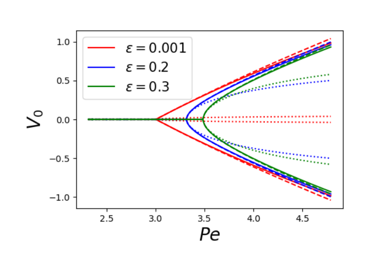
Generally, in nonlinear systems an exact solution is the exception. The traditional way is then to expand the model equations in power series in an amplitude (denoted here as ) to obtain the final result in the form (15). The present study shows that wee can extract from the traditional expansion thee results (15) (18) and (19), the correct singular behavior and the appropriate regularized form when is small but finite. This highlights the generality of the method and its application to various nonlinear systems with a hidden singularity.
Let us finally briefly classify singular bifurcations on the basis of the behavior of the general traditional expansion (15). Suppose that the singularity is due to the presence of terms of the form where is real non integer positive number such that . Following the general procedure presented above, we straightforwardly obtain to leading order
| (20) |
where is a real number, and where we have rescaled so that the coefficient in front of the singular term can be set to unity. If the first dominant term is and to leading order the expansion is regular. Note that we have assumed the first nonlinear term to saturate the linear growth, this is why we set its coefficient to be negative. In the opposite case higher order terms (such as ) must be taken into account). This question is beyond our scope here. In terms of a dynamical system, and by remembering that we assume to exist always as a solution, the corresponding normal form is
| (21) |
with . Equation (21) constitutes the generic normal form for singular bifurcation. We used here the notation , as often adopted in bifurcation theory. The nontrivial fixed point behaves as . The bifurcation structure is qualitatively different depending on whether or . In the first case the bifurcation diagram is similar to a pitchfork bifurcation with infinite slope at , whereas in the second case the slope vanishes for . is a special case with finite slope. Finally for the normal form is
| (22) |
We adopted the positive sign in front of the nonlinear term to guarantee a stable branch for . Note that this does not affect the bifurcation diagram topology. The nontrivial fixed point is given . Figure 2 summarizes the results. We note four different singular bifurcations (in blue in Fig.2) corresponding to (i) , (ii) , (iii) , (iv) . We refer to these four singular bifurcations as (i) fold, (ii) cusp, (iii) angular and (iv) unbounded. When these bifurcations are regularized, they all fall into a pitchfork bifurcation (Figure 2). We may refer to the above bifurcations as singular pitchfork bifurcations as well, albeit the singular limits have different behaviors. It must be noted that the above classification does not exhaust by far all kinds of singularities. For example, the 2D phoretic model provides an example of transcendental singularity where the velocity behaves as SM.


Some important remarks are in order. We have assumed that the singularity of lies on the imaginary axis, . Note, however, that it can happen (as in the phoretic model with finite size; see SM) that there exists an infinite countable set of singularities on the imaginary axis. It is also not excluded that there may be systems with several singularities scattered in the complex plane, for which no general theory is at present available. However, in SM we provide a condition of validity of the theory even when singularity does not lie on the imaginary axis.
Conclusion–
We have provided a framework to deal with singular bifurcations. The few concrete examples mentioned in the introduction are far from having exhausted all cases where singular bifurcations manifest themeselves. Suzade et al Sauzade et al. 2011 analyzed the speed of the Taylor swimmer sheet in perturbation theory as a function amplitude of the swimmer deformation by including up to 1000 terms in the series expansion. They found that the series diverges beyond an amplitude of deformation (which is moderate). This is symptomatic of a hidden singularity in the model. In another problem, that of vesicles (a simple model of red blood cells) in a flow Farutin et al. 2012; Farutin and Misbah 2013, the perturbative schemes for vesicle dynamics (in power series of excess area from a sphere) has a small range of applicability even when including higher and higher order terms in the series expansion. This is indicative of potential singularity in complex plane. It is hoped that this study serves as a general framework to analyze singular bifurcations.
We thank CNES (Centre National d’Etudes Spatiales) for financial support and for having access to data of microgravity, and the French-German university programme ”Living Fluids” (Grant CFDA-Q1-14) for financial support.
References
- Cross and Hohenberg (1993) M. C. Cross and P. C. Hohenberg, Rev. Mod. Phys. 65, 851 (1993).
- Hoyle (2010) R. Hoyle, Pattern Formation An Introduction to Methods (Cambridge University Press, 2010).
- Misbah (2017) C. Misbah, Complex Dynamics and Morphogenesis (Springer, Berlin, 2017).
- Cross and Greenside (2012) M. Cross and H. Greenside, Pattern Formation and Dynamics in Nonequilibrium Systems (Cambridge University Press, 2012).
- Goluskin (2015) D. Goluskin, Internally Heated Convection and Rayleigh-Benard Convection (Springer Berlin, 2015).
- Turing (1951) A. M. Turing, Phil. Trans. R. Soc. Lond. B 273, 37 (1951).
- Bourgine and Lesne (2011) P. Bourgine and A. Lesne, Morphogenesis Origin of Shape and Patterns (Springer, 2011).
- Kassner (1996) K. Kassner, Pattern Formation in Diffusion-Limited Crystal Growth: Beyond the Single Dendrite (World Scientific, 1996).
- Saito (1996) Y. Saito, Statistical Physics Of Crystal Growth (World Scientific, 1996).
- Misbah et al. (2010) C. Misbah, O. Pierre-Louis, and Y. Saito, Rev. Mod. Phys. 82, 981 (2010).
- Hof et al. (2004) B. Hof, C. W. H. van Doorne, J. Westerweel, F. T. M. Nieuwstadt, H. Faisst, B. Eckhardt, H. Wedin, R. R. Kerswell, and F. Waleffe, Science 305, 1594 (2004).
- Thom (2018) R. Thom, Structural Stability and Morphogenesis (CRC Press, 2018).
- Izri et al. (2014) Z. Izri, M. N. Van Der Linden, S. Michelin, and O. Dauchot, Phys. Rev. Lett. 113, 248302 (2014).
- Michelin et al. (2013) S. Michelin, E. Lauga, and D. Bartolo, Phys. Fluids 25, 061701 (2013).
- Rednikov et al. (1994) A. Y. Rednikov, Y. S. Ryazantsev, and M. G. Velarde, Physics of Fluids 6, 451 (1994).
- Jin et al. (2017) C. Jin, C. Krüger, and C. C. Maass, Proceedings of the National Academy of Sciences 114, 5089 (2017), https://www.pnas.org/content/114/20/5089.full.pdf .
- Hu et al. (2019) W. F. Hu, T. S. Lin, S. Rafai, and C. Misbah, Phys. Rev. Lett. 123, 238004 (2019).
- Morozov and Michelin (2019a) M. Morozov and S. Michelin, J. Chem. Phys. 150, 044110 (2019a).
- Izzet et al. (2020) A. Izzet, P. G. Moerman, P. Gross, J. Groenewold, A. D. Hollingsworth, J. Bibette, and J. Brujic, Phys. Rev. X 10, 021035 (2020).
- Hokmabad et al. (2021) B. V. Hokmabad, R. Dey, M. Jalaal, D. Mohanty, M. Almukambetova, K. A. Baldwin, D. Lohse, and C. C. Maass, Phys. Rev. X 11, 011043 (2021).
- Chen et al. (2021) Y. Chen, K. L. Chong, L. Liu, R. Verzicco, and D. Lohse, Journal of Fluid Mechanics 919, A10 (2021).
- Morozov and Michelin (2019b) M. Morozov and S. Michelin, Journal of Fluid Mechanics 860, 711 (2019b).
- Saha et al. (2021) S. Saha, E. Yariv, and O. Schnitzer, Journal of Fluid Mechanics 916, A47 (2021).
- Pierre-Louis et al. (1998) O. Pierre-Louis, C. Misbah, Y. Saito, J. Krug, and P. Politi, Phys. Rev. Lett. 80, 4221 (1998).
- (25) See supplemental material at [URL will be inserted by publisher] .
- Sauzade et al. (2011) M. Sauzade, G. J. lfring, and E. Lauga, Physica D 240, 1567 (2011).
- Farutin et al. (2012) A. Farutin, O. Aouane, and C. Misbah, Phys. Rev. E 85, 061922 (2012).
- Farutin and Misbah (2013) A. Farutin and C. Misbah, Phys. Rev. Lett. 110, 108104 (2013).
Supplemental Materials: Singular Bifurcations: a Regularization Theory
Supplementary Information: Singular Bifurcations : a Regularization Theory
August 11, 2026
We provide here the regularization solution for the phoretic model for finite size in 3D. We also present the singular behavior in 2D, which is quite distinct from that in 3D. More details about the results discussed in the main text are also presented.
I Effect of hydrodynamics on critical condition
The goal of this section is to introduce the corrections into the exactly solvable model in order to account for the finite size of the particle. These corrections are evaluated for small propulsion velocity and provide quantitatively correct value of the critical Peclet number. There are two finite-size effects that are neglected in the main model: First, the near-field flow disturbance due to a translating spherical particle is neglected, and second, the particle emission is represented by a point source, while the finite-size particle should be represented by a homogeneous distribution of sources along the particle surface. Both of these two effects are essential for quantitative evaluation of the concentration field close to the critical point.
This problem is solved in the reference frame comoving with the particle. The concentration evolution equation is then written as
| (S1) |
where is the fluid velocity relative to the particle, represents a distribution of sources and source dipoles on the particle surface which accounts for the concentration emission or consumption, and is the position vector relative to the particle center. It is known that the velocity field in the comoving frame can be written as
| (S2) |
for a rigid force-free spherical particle or radius , moving with velocity relative to the laboratory frame. The flow field in eq. (S2) can be written in potential representation , where
| (S3) |
We also have for due to the flow incompressibility.
We focus on the steady-state solution of Eq. (S1). Multiplying eq. (S1) by , yields
| (S4) |
where and .
The original model corresponds to setting to , to , and to a point source in eq. (S4). Here we still simplify to because this term is quadratic in velocity and thus should be small close to the critical point. We keep, however, the full expression for and replace the term with a combination of a point source and a point source dipole. The amplitude of the source dipole is chosen in a way that corresponds to an isotropic emission rate at distance from the particle center.
We thus consider the following equation
| (S5) |
This equation can be solved analytically, yielding
| (S6) |
The constant is found by taking the concentration field and setting the first harmonic of to zero:
| (S7) |
where . Substituting eq. (S7) into eq. (S6) yields the corrected concentration field. We extract the first harmonic of the concentration for from this solution, which gives us the following expression of the swimming velocity
| (S8) |
Dividing both sides of eq. S8 by and setting to 0 yields for the critical Peclet number, which agrees with the previous works.
II Finite size effect
We consider the same phoretic model except that the size is finite. We focus here only on steady state solutions in the co-moving frame with velocity . The concentration field obeys in this frame
| (S9) |
The particle is taken to move along the direction. Making the substitution we find
| (S10) |
This is the so-called screened Helmotz equation with a delta source term. The associated Green’s function is defined as
| (S11) |
We consider the domain to be finite and bounded by a sphere with radius (counted from the point source). The boundary condition is taken as . We use the eigenfunctions of the Laplacian in order to express the Green’s function. The Laplacian eigenfunctions are spherical harmonics times spherical Bessel functions . Let define the zero’s of , we have . The Laplacian eigenfunction which vanishes at can be written as
| (S12) |
Then making use of the classical method to express the Green’s function in terms of eigenfunctions, we obtain
| (S13) |
Note that the eigenvalues of the Laplacian are , meaning that the eigenvalues of the full operator in (S10) are . The above Green’s function can be rewritten as
| (S14) |
after having used the addition theorem for spherical harmonics, where is the Legendre polynomial of order and . Since the source term is assumed to be at the center, we set , so that . Due to the properties of only survives in the sum. Using the definition of and functions, we obtain (upon using that ) that the concentration field can be written as
| (S15) |
where we have used the result , being the hyperbolic cosecant function. Projecting on the first spherical harmonic, and using the condition that (recall that is the concentration contribution of the first harmonic at ) we find
| (S16) |
where . Expanding this result for small we obtain to cubic order
| (S17) |
We see that the expansion is regular; the finite size has regularized the singular pitchfork behavior. The solution always exists. Beyond a certain critical value there exists another solution behaving as , with . If we take first the limit in Eq. (S16), we obtain
| (S18) |
yielding the same expression as in the main text for infinite size. The function has a infinite and countable set of singularities on the imaginary axis, , being an integer.
III Relation between and
It is easy to obtain the general relation between and . However here we only list the relations for the first three terms (generalization to arbitrary order is straightforward). The starting point is to write the Taylor expanion in terms of and makes the substitution and , so that we have
| (S19) |
Then expansing in Taylor series with respect to , we obtain to leading order
| (S20) |
with the relations
| (S21) |
where as well as and , which designate first and second derivative with respect to , are evaluated at .
IV 2D model with consumption
In 2D we only need to substitute in the denominator of the propagator by , so that the concentration field takes the form
| (S22) |
.
yielding
| (S23) |
where , and is the Bessel function of the second kind. Projecting (S17) on the first Fourier mode and using the equation fixing velocity as a function of concentration (see main text) we find (where is the amplitude of the first Fourier mode), obtaining finally
| (S24) |
where is the Bessel function of the first kind. Besides the trivial solution, this equation exhibits a pitchfork bifurcation. For the bifurcation becomes singular with ; for a small argument and .
V Singularities outside of the imaginary axis
Here we discuss the applicability of the method for the problems in which the singularities are not necessary on the imaginary axis. Suppose there is a function , where is the expansion parameter and is the regularization parameter, as in the Main Letter. The function is an analytic function of with exception of singular points . Here we allow to be arbitrary complex numbers. Applying the transformation and , we obtain a function of and . This function is an analytical function of with exception of singular points given by
| (S25) |
The radius of convergence of the expansion of in powers of is governed by the singular point with the lowest absolute value. The success of the proposed method requires this radius of convergence to be greater than 1. The method thus works if all are such that , where is given by (S25). Figure S1 shows the region of the complex plane which must contain for all singular points of in order for the expansion in to converge for .
