跳到论文正文
W Papers独立论文阅读器 arXiv:2112.12048 论文正文 计算阅读时间 · 0%
引用这篇论文根据当前论文元数据生成,正式投稿前建议核对。


License: arXiv.org perpetual non-exclusive license
arXiv:2112.12048v1 [gr-qc] 22 Dec 2021
\IDnumber

1706626 \courseFisica \courseorganizerFacoltà di Scienze Matematiche, Fisiche e Naturali \AcademicYear2019/2020 \copyyear2020 \advisorProf. Paolo Pani \coadvisorDr. Taishi Ikeda \authoremailfabrizio.corelli@uniroma1.it \versiondate22nd December 2021

Instability of Schwarzschild Black Holes in Einstein-scalar-Gauss-Bonnet Gravity: Perturbative Approach and Time-Domain Analysis

Fabrizio Corelli
Abstract

We study the instability of Schwarzschild black holes and the appearance of scalarized solutions in Einstein-scalar-Gauss-Bonnet gravity performing a time-domain analysis in a perturbative scheme. First we consider a quadratic coupling function and we perform an expansion for a small perturbation of the scalar field around the Schwarzschild solution up to the second order; we do not observe any stable scalarized configuration, in agreement with previous studies. We then consider the cases of quartic and exponential coupling, using an expansion for small values of the Newton’s constant, in order to include the nonlinear terms introduced by the coupling in the field equations; in this case we observe the appearance of stable scalarized solutions different from those found in literature. The discrepancy can be an artifact of the perturbative approach.

Chapter 1 Introduction

General Relativity was introduced by Albert Einstein in 1915. It represents one of the most important theories of the last century, and has been widely tested in the range of lenghts 1​μ​m≲l≲1011​m1\,\mu m\lesssim l\lesssim 10^{11}\,m. In particular the recent observations of binary black hole mergers and binary neutron star mergers have provided excellent confirmations of the predictions of the Einstein’s theory of gravity.
However there are some critical aspects from a theoretical and cosmological point of view that suggest to investigate alternative theories of gravity. For instance, it can be shown that General Relativity is not renormalizable and therefore it cannot be easily treated from quantum field theory point of view. Moreover, the accelerated expansion of the universe leads to the introduction of dark energy, which can be explained with a nonzero cosmological constant. However, the measurements of the cosmological constant from experimental observations are in contrast with the estimations of the zero-point energy obtained by quantum field theory computations.

An interesting way to extend General Relativity is to introduce a dynamical scalar field in the action; in this case the equations for the metric contain also the scalar field and they are different from the Einstein’s equations. When the scalar field is nonminimally coupled to gravity the theory goes under the name of scalar-tensor gravity.
A critical issue of scalar-tensor theories is that the field equations can be of order higher than two. This can lead to the appearance of a ghost-like instability called Ostrogradsky instability. However this phenomenon can be avoided by considering the so called Horndeski theories, which are the most general scalar-tensor theories whose field equations are of order two.
Another interesting theory is quadratic gravity, in which the action contains quadratic terms in the curvature, and it can be considered as a low-energy approximation of a more general action in a quantum field theory model that includes gravity.

In this work we are going to study Einstein-scalar-Gauss-Bonnet (EsGB) gravity, in which the coupling between the scalar field and the metric is given by a coupling function multiplied by the Gauss-Bonnet invariant 𝒢=R2−4​Rμ​ν​Rμ​ν+Rμ​ν​α​β​Rμ​ν​α​β\mathcal{G}=R^{2}-4R_{\mu\nu}R^{\mu\nu}+R_{\mu\nu\alpha\beta}R^{\mu\nu\alpha\beta}. This theory belongs simultaneously to the classes of Horndeski and quadratic gravity.
The corrections of EsGB gravity to General Relativity are in the high curvature/energy regime and it is interesting to analyze the characteristics of compact objects, in particular black holes.

Thanks to the no-hair theorem in General Relativity black holes are described by the Kerr-Newman metric, which is defined using only three quantities: mass, angular momentum and electric charge. This theorem is very stringent and expresses a conceptual simplicity in the description of black holes, that can be used to test the validity of an alternative theory of gravity: the eventual observation of deviations from the predictions of the no-hair theorem can give a confirmation to a theory that introduces auxiliary quantities for the description of the black hole metric. Moreover, even if these deviations are absent, the prediction of a theory of modified gravity can be useful to understand from an observational point of view how the no-hair theorem operates and why it is not violated.

In some EsGB gravities when the scalar field assumes a trivial configuration, the black hole solution reduces to the one predicted by General Relativity. Nevertheless there are choices of the coupling function for which the scalar field can assume nontrivial configurations that require additional constants (usually referred as “hairs”) to be described.
Recently a new phenomenon called spontaneous black hole scalarization has been found to occur in EsGB gravity (refs. [42, 44]). This phenomenon is the analog of the spontaneous scalarization introduced in the 90’s by Damour and Esposito-Farèse for neutron stars (refs. [45, 46]), and it consists in the development of an instability in the trivial solution of the scalar field and in the appearance of stable nontrivial configurations. The additional parameter required to describe the black hole solutions is called scalar charge, while the nontrivial configurations of the scalar field are called scalarized solutions.
From an observational point of view, the effects of the presence of the scalar charge may be seen in gravitational waves. In fact a binary system of scalarized black holes possesses a scalar dipole moment that, rotating, emits scalar dipole radiation, affecting the gravitational wave signal (see e.g. ref. [25]).
Spontaneous scalarization has been studied for quadratic, quartic and exponential coupling functions in the case of massless scalar field. It has been found that for certain choices of the parameters in the coupling function the Schwarzschild solution is unstable, and there are scalarized solutions that can be classified by the number of nodes and the scalar charge. In the case of quadratic coupling function there are not stable scalarized solutions, while in the other two cases there are stable nontrivial configurations of the scalar field, and the scalarized solutions with n≥1n\geq 1 nodes are unstable. According to ref. [49] this behavior is related to the presence of nonlinear terms in the equation for the scalar field. In fact the quadratic term of the coupling function contributes with a linear term in the equation, and the higher order terms in the coupling function provide nonlinear terms that can quench the instability. In the case of quadratic coupling these nonlinear terms are absent and the scalarized solutions are unstable.
In recent years spontaneous scalarization has also been studied for charged black holes (see refs. [52, 53]), for massive scalar field (see refs. [51, 47]) and for spinning black holes (see refs. [54, 55]). We will not analyze these studies, but we will focus only on the spherically symmetric case with massless scalar field.

In this work we will study the instability of a Schwarzschild black hole and the appearance of stable scalarized solutions in some EsGB gravities performing a time-domain analysis in a perturbative scheme. The time-domain approach allows us to delineate the evolution of the solutions, to study how the instability appears, and how the stable configurations are reached.
In order to compute the time evolution of the system we developed a 1+1 code in C for the numerical integration of time dependent partially differential equations with a constraint.
In the first part we are going to consider a quadratic coupling function F⁡[ϕ]=λ​ϕ2F[\phi]=\lambda\phi^{2}, where ϕ\phi is the scalar field and λ\lambda is a coupling constant. We will assume ϕ\phi as a small perturbation around the Schwarzschild solution and then we will expand up to the second order in the field equations. In this approximation we can consider the effects of the backreaction of the scalar field on the metric, and the equation for ϕ\phi can be integrated using the Schwarzschild metric as background. This remarkable simplification in the field equations is the point of strength of the perturbative approach.
Our intent is to determine the values of the coupling parameter λ\lambda for which the Schwarzschild solution is stable and to characterize the instability. We will also discuss the possibility of studying the evolution of the position of the apparent horizon in this perturbative scheme.

Then we are going to consider the instability of a Schwarzschild black hole with a quartic coupling function F⁡[ϕ]=λ​ϕ2+γ​ϕ4F[\phi]=\lambda\phi^{2}+\gamma\phi^{4}. In this case the equation for the scalar field contains nonlinear terms in ϕ\phi, and stable nodeless scalarized solutions have been found, therefore it is interesting to study how the instability of the Schwarzschild solution is quenched and how the scalar field reaches a nontrivial stable configuration.
However the perturbative scheme we are going to use for the quadratic coupling function cannot be used with the quartic coupling. In fact, expanding in a perturbation of the scalar field, the terms that come from ϕ4\phi^{4} do not appear in the equations at the second order. Therefore we will perform an expansion for a small Newton’s constant GG, in such a way that we can treat the linear and the nonlinear terms in the equation for the scalar field at the same order in perturbation theory.
We will determine with a time-domain analysis the ranges of values for the parameters λ\lambda and γ\gamma where the Schwarzschild solution is unstable, we will discuss the appearance of stable scalarized solutions and compute their scalar charge.
We will also consider the case of exponential coupling F⁡[ϕ]=λ3​(1−e−3​ϕ2)F[\phi]=\frac{\lambda}{3}\Bigl(1-e^{-3\phi^{2}}\Bigr) using the expansion in the Newton’s constant. As in the case of quartic coupling, the equation for the scalar field contains nonlinearities and stable scalarized solutions appear.

The structure of the thesis is the following.
In chapter 2 we will discuss the reasons to introduce modifications in General Relativity and a scheme to classify the alternative theories on the basis of the violation of the Lovelock’s theorem, following the structure of ref. [23]. We will introduce scalar-tensor theories, Horndeski theories and quadratic gravity, arriving then to Einstein-scalar-Gauss-Bonnet gravity. We will explore the no-hair theorem in General Relativity, and some extensions in scalar-tensor theories, analyzing in detail the case of EsGB gravity. Finally we will discuss the phenomenon of spontaneous scalarization, and we will review some results obtained in recent years.
In chapter 3 we will analyze the case of quadratic coupling function. We will perform the expansion for a perturbation around the trivial configuration of the scalar field, and we will integrate numerically the equations analyzing the stability of the solutions. We will then compute the evolution of the position of the apparent horizon and discuss the possibility of studying it in the perturbative scheme.
In chapter 4 and 5 we will consider respectively the quartic and the exponential couplings with the expansion in the Newton’s constant, analyzing the stability of the scalarized solutions and computing their scalar charge.
The thesis ends with the conclusions in chapter 6.

Chapter 2 Modifications of General Relativity and Hairy Black Holes

In this chapter we will discuss some possible approaches for extending General Relativity. In particular we will describe scalar-tensor theories and quadratic gravity, and we will focus on EsGB gravity. We will discuss about possible extensions of the no-hair theorems in EsGB gravity, and the occurrence of the so called spontaneous scalarization, reporting some results obtained in recent years.
In the first part of the chapter we will follow the presentation in ref. [23].

2.1 Necessity for a Modification of General Relativity

General Relativity (GR) has received several confirmations during the last century, from the deflection of light discovered by Arthur Eddington in 1919 [1] to the recent detections of gravitational waves from binary systems by the LIGO-Virgo collaboration starting from 2015 [2, 3, 4, 5, 6, 7, 8, 9, 10, 11] and the image of a black hole with its shadow obtained in 2019 by the EHT collaboration [12, 13, 14, 15, 16, 17].
However, there are reasons to investigate possible modifications of GR, and they come mainly from theoretical and cosmological arguments.
From a theoretical perspective the main issue is the classical nature of General Relativity. Using the renormalizability criterion it can be shown that GR is a non-renormalizable theory; in fact the dimension of the coupling constant in natural units (ℏ=c=1\hbar=c=1) are given by the dimensions of the gravitational constant, which are [G]=[E−2][G]=[E^{-2}] (see ref. [18]). Therefore GR cannot be included in a quantum field theory description of the universe.
At the same time, the discovery of the accelerated expansion of the universe in 1998 [20] highlighted new criticalities from a cosmological point of view. In GR this phenomenon can be described with a positive cosmological constant11 1 See also ref. [19] for a review on the Dark Energy and the accelerated expansion of the universe. [21], whose evaluation poses new critical issues in the context of the General Relativity and the Standard Model of particle physics, such as the cosmological constant problem (or vacuum catastrophe), which is the discrepancy between the measured value of the cosmological constant and the quantum field theory prediction of the zero-point energy [22].
A modified version of General Relativity must include correction at low or high energies, while it must reduce to GR in the intermediate energy regime, in order to be consistent with the current experimental results. In particular, the length scale where GR has been tested is 1​μ​m≲l≲1011​m1\,\mu m\lesssim\mathit{l}\lesssim 10^{11}\,m (see ref. [23]) and the corrections must appear out of this range. Corrections at high energy and small length scales are called ultraviolet (UV) corrections, whose effects can appear in astrophysical compact objects, such as Black Holes (BH) and Neutron Stars (NS), while corrections at low energy and long length scales are called infrared (IR) corrections, and they can be investigated by examining cosmological phenomena and also from the gravitational waves (see e.g. [24]).

2.2 Lovelock’s Theorem and Possible Modifications of GR

Let us now delineate a possible scheme to introduce modifications in GR. This scheme is described in detail in ref. [23], and we are going to summarize it without dwelling on the illustration of all the theories referable to it. According to Lovelock’s theorem [26], in four dimensions any rank-2 symmetric tensor Aμ​ν=Aν​μA^{\mu\nu}=A^{\nu\mu} with null divergence A;νμ​ν​\mathchoice{A^{{{\mu\nu}\mathchoice{\makebox[7.63892pt][c]{$\displaystyle$}}{\makebox[7.63892pt][c]{$\textstyle$}}{\makebox[3.78163pt][c]{$\scriptstyle$}}{\makebox[2.70114pt][c]{$\scriptscriptstyle$}}}}_{{\mathchoice{\makebox[8.8716pt][c]{$\displaystyle$}}{\makebox[8.8716pt][c]{$\textstyle$}}{\makebox[5.373pt][c]{$\scriptstyle$}}{\makebox[3.83784pt][c]{$\scriptscriptstyle$}}{;\nu}}}}{A^{{{\mu\nu}\mathchoice{\makebox[7.63892pt][c]{$\displaystyle$}}{\makebox[7.63892pt][c]{$\textstyle$}}{\makebox[3.78163pt][c]{$\scriptstyle$}}{\makebox[2.70114pt][c]{$\scriptscriptstyle$}}}}_{{\mathchoice{\makebox[8.8716pt][c]{$\displaystyle$}}{\makebox[8.8716pt][c]{$\textstyle$}}{\makebox[5.373pt][c]{$\scriptstyle$}}{\makebox[3.83784pt][c]{$\scriptscriptstyle$}}{;\nu}}}}{A^{{{\mu\nu}\mathchoice{\makebox[7.63892pt][c]{$\displaystyle$}}{\makebox[7.63892pt][c]{$\textstyle$}}{\makebox[3.78163pt][c]{$\scriptstyle$}}{\makebox[2.70114pt][c]{$\scriptscriptstyle$}}}}_{{\mathchoice{\makebox[8.8716pt][c]{$\displaystyle$}}{\makebox[8.8716pt][c]{$\textstyle$}}{\makebox[5.373pt][c]{$\scriptstyle$}}{\makebox[3.83784pt][c]{$\scriptscriptstyle$}}{;\nu}}}}{A^{{{\mu\nu}\mathchoice{\makebox[7.63892pt][c]{$\displaystyle$}}{\makebox[7.63892pt][c]{$\textstyle$}}{\makebox[3.78163pt][c]{$\scriptstyle$}}{\makebox[2.70114pt][c]{$\scriptscriptstyle$}}}}_{{\mathchoice{\makebox[8.8716pt][c]{$\displaystyle$}}{\makebox[8.8716pt][c]{$\textstyle$}}{\makebox[5.373pt][c]{$\scriptstyle$}}{\makebox[3.83784pt][c]{$\scriptscriptstyle$}}{;\nu}}}}, constructed only from the metric tensor gμ​νg^{\mu\nu} and its first and second order derivatives, and which preserves diffeomorphism invariance, can be written as a linear combination of the Einstein tensor Gμ​ν=Rμ​ν−12​R​gμ​νG^{\mu\nu}=R^{\mu\nu}-\frac{1}{2}Rg^{\mu\nu} and gμ​νg^{\mu\nu}:

Aμ​ν=α​Gμ​ν+β​gμ​ν.A^{\mu\nu}=\alpha G^{\mu\nu}+\beta g^{\mu\nu}. (2.1)

This leads to the Einstein’s equations with the addiction of a cosmological term

Gμ​ν+Λ​gμ​ν=8​π​Gc4​Tμ​ν,G_{\mu\nu}+\Lambda g_{\mu\nu}=\frac{8\pi G}{c^{4}}T_{\mu\nu}, (2.2)

where Tμ​νT_{\mu\nu} is the matter stress-energy tensor and Λ\Lambda is the cosmological constant.
In order to modify GR we have to violate one or more hypotheses of the Lovelock’s theorem. We are now going to list some possible violations of the postulates, following ref. [23], and some theories proposed.

  1. 1.

    Violation of the hypothesis that Aμ​νA^{\mu\nu} must be constructed only with gμ​νg^{\mu\nu} and its first and second derivatives.

    This hypothesis can be violated by adding a field, which can be either dynamical and nondynamical. In the case of dynamical field we can add in the left hand side of the Einstein’s equations some couplings between the metric tensor and the field [23]. Einstein-scalar-Gauss-Bonnet (EsGB) gravity belongs to this class of theories. Instead in the case of nondynamical field the aim is to write the Einstein’s equations with Gμ​νG_{\mu\nu} on the left hand side, and, on the right hand side, a nonlinear combination of a stress-energy tensor that satisfies the condition T;νμ​ν​=0\mathchoice{T^{{{\mu\nu}\mathchoice{\makebox[7.63892pt][c]{$\displaystyle$}}{\makebox[7.63892pt][c]{$\textstyle$}}{\makebox[3.78163pt][c]{$\scriptstyle$}}{\makebox[2.70114pt][c]{$\scriptscriptstyle$}}}}_{{\mathchoice{\makebox[8.8716pt][c]{$\displaystyle$}}{\makebox[8.8716pt][c]{$\textstyle$}}{\makebox[5.373pt][c]{$\scriptstyle$}}{\makebox[3.83784pt][c]{$\scriptscriptstyle$}}{;\nu}}}}{T^{{{\mu\nu}\mathchoice{\makebox[7.63892pt][c]{$\displaystyle$}}{\makebox[7.63892pt][c]{$\textstyle$}}{\makebox[3.78163pt][c]{$\scriptstyle$}}{\makebox[2.70114pt][c]{$\scriptscriptstyle$}}}}_{{\mathchoice{\makebox[8.8716pt][c]{$\displaystyle$}}{\makebox[8.8716pt][c]{$\textstyle$}}{\makebox[5.373pt][c]{$\scriptstyle$}}{\makebox[3.83784pt][c]{$\scriptscriptstyle$}}{;\nu}}}}{T^{{{\mu\nu}\mathchoice{\makebox[7.63892pt][c]{$\displaystyle$}}{\makebox[7.63892pt][c]{$\textstyle$}}{\makebox[3.78163pt][c]{$\scriptstyle$}}{\makebox[2.70114pt][c]{$\scriptscriptstyle$}}}}_{{\mathchoice{\makebox[8.8716pt][c]{$\displaystyle$}}{\makebox[8.8716pt][c]{$\textstyle$}}{\makebox[5.373pt][c]{$\scriptstyle$}}{\makebox[3.83784pt][c]{$\scriptscriptstyle$}}{;\nu}}}}{T^{{{\mu\nu}\mathchoice{\makebox[7.63892pt][c]{$\displaystyle$}}{\makebox[7.63892pt][c]{$\textstyle$}}{\makebox[3.78163pt][c]{$\scriptstyle$}}{\makebox[2.70114pt][c]{$\scriptscriptstyle$}}}}_{{\mathchoice{\makebox[8.8716pt][c]{$\displaystyle$}}{\makebox[8.8716pt][c]{$\textstyle$}}{\makebox[5.373pt][c]{$\scriptstyle$}}{\makebox[3.83784pt][c]{$\scriptscriptstyle$}}{;\nu}}}}=0, in such a way that the weak equivalence principle holds. A theory of this type is the Palatini f⁡(ℛ)f(\mathcal{R}) gravity [23].

  2. 2.

    Violation of the hypothesis of a 4 dimensional spacetime.

    This hypothesis is violated by considering the number of dimensions as a parameter of the theory. This could be interesting in order to study how the theory depends on the number of dimensions, and also in the context of string theory. An example of higher dimensional theory is the Kaluza-Klein gravity [23].

  3. 3.

    Violation of the diffeomorphism invariance hypothesis.

    Two common ways of violating the diffeomorphism invariance are to break Lorentz invariance or to consider a model of massive gravity. In the first case the idea is that Lorentz symmetry is broken at high energy and hence this type of theory can provide UV corrections to GR. A Lorentz violating theory is, for instance, Einstein-Æther gravity [23]. Instead in the second case the idea is to consider a massive graviton, i.e. a massive spin-2 field. An example of massive gravity theory is de Rham-Gabadadze-Tolley (dRGT) gravity [23].

  4. 4.

    Violation of the hypothesis A;νμ​ν​=0\mathchoice{A^{{{\mu\nu}\mathchoice{\makebox[7.63892pt][c]{$\displaystyle$}}{\makebox[7.63892pt][c]{$\textstyle$}}{\makebox[3.78163pt][c]{$\scriptstyle$}}{\makebox[2.70114pt][c]{$\scriptscriptstyle$}}}}_{{\mathchoice{\makebox[8.8716pt][c]{$\displaystyle$}}{\makebox[8.8716pt][c]{$\textstyle$}}{\makebox[5.373pt][c]{$\scriptstyle$}}{\makebox[3.83784pt][c]{$\scriptscriptstyle$}}{;\nu}}}}{A^{{{\mu\nu}\mathchoice{\makebox[7.63892pt][c]{$\displaystyle$}}{\makebox[7.63892pt][c]{$\textstyle$}}{\makebox[3.78163pt][c]{$\scriptstyle$}}{\makebox[2.70114pt][c]{$\scriptscriptstyle$}}}}_{{\mathchoice{\makebox[8.8716pt][c]{$\displaystyle$}}{\makebox[8.8716pt][c]{$\textstyle$}}{\makebox[5.373pt][c]{$\scriptstyle$}}{\makebox[3.83784pt][c]{$\scriptscriptstyle$}}{;\nu}}}}{A^{{{\mu\nu}\mathchoice{\makebox[7.63892pt][c]{$\displaystyle$}}{\makebox[7.63892pt][c]{$\textstyle$}}{\makebox[3.78163pt][c]{$\scriptstyle$}}{\makebox[2.70114pt][c]{$\scriptscriptstyle$}}}}_{{\mathchoice{\makebox[8.8716pt][c]{$\displaystyle$}}{\makebox[8.8716pt][c]{$\textstyle$}}{\makebox[5.373pt][c]{$\scriptstyle$}}{\makebox[3.83784pt][c]{$\scriptscriptstyle$}}{;\nu}}}}{A^{{{\mu\nu}\mathchoice{\makebox[7.63892pt][c]{$\displaystyle$}}{\makebox[7.63892pt][c]{$\textstyle$}}{\makebox[3.78163pt][c]{$\scriptstyle$}}{\makebox[2.70114pt][c]{$\scriptscriptstyle$}}}}_{{\mathchoice{\makebox[8.8716pt][c]{$\displaystyle$}}{\makebox[8.8716pt][c]{$\textstyle$}}{\makebox[5.373pt][c]{$\scriptstyle$}}{\makebox[3.83784pt][c]{$\scriptscriptstyle$}}{;\nu}}}}=0.

    In this case the general idea is that if we violate the Weak Equivalence Principle (WEP), then condition T;νμ​ν​=0\mathchoice{T^{{{\mu\nu}\mathchoice{\makebox[7.63892pt][c]{$\displaystyle$}}{\makebox[7.63892pt][c]{$\textstyle$}}{\makebox[3.78163pt][c]{$\scriptstyle$}}{\makebox[2.70114pt][c]{$\scriptscriptstyle$}}}}_{{\mathchoice{\makebox[8.8716pt][c]{$\displaystyle$}}{\makebox[8.8716pt][c]{$\textstyle$}}{\makebox[5.373pt][c]{$\scriptstyle$}}{\makebox[3.83784pt][c]{$\scriptscriptstyle$}}{;\nu}}}}{T^{{{\mu\nu}\mathchoice{\makebox[7.63892pt][c]{$\displaystyle$}}{\makebox[7.63892pt][c]{$\textstyle$}}{\makebox[3.78163pt][c]{$\scriptstyle$}}{\makebox[2.70114pt][c]{$\scriptscriptstyle$}}}}_{{\mathchoice{\makebox[8.8716pt][c]{$\displaystyle$}}{\makebox[8.8716pt][c]{$\textstyle$}}{\makebox[5.373pt][c]{$\scriptstyle$}}{\makebox[3.83784pt][c]{$\scriptscriptstyle$}}{;\nu}}}}{T^{{{\mu\nu}\mathchoice{\makebox[7.63892pt][c]{$\displaystyle$}}{\makebox[7.63892pt][c]{$\textstyle$}}{\makebox[3.78163pt][c]{$\scriptstyle$}}{\makebox[2.70114pt][c]{$\scriptscriptstyle$}}}}_{{\mathchoice{\makebox[8.8716pt][c]{$\displaystyle$}}{\makebox[8.8716pt][c]{$\textstyle$}}{\makebox[5.373pt][c]{$\scriptstyle$}}{\makebox[3.83784pt][c]{$\scriptscriptstyle$}}{;\nu}}}}{T^{{{\mu\nu}\mathchoice{\makebox[7.63892pt][c]{$\displaystyle$}}{\makebox[7.63892pt][c]{$\textstyle$}}{\makebox[3.78163pt][c]{$\scriptstyle$}}{\makebox[2.70114pt][c]{$\scriptscriptstyle$}}}}_{{\mathchoice{\makebox[8.8716pt][c]{$\displaystyle$}}{\makebox[8.8716pt][c]{$\textstyle$}}{\makebox[5.373pt][c]{$\scriptstyle$}}{\makebox[3.83784pt][c]{$\scriptscriptstyle$}}{;\nu}}}}=0 does not hold anymore and the hypothesis A;νμ​ν​=0\mathchoice{A^{{{\mu\nu}\mathchoice{\makebox[7.63892pt][c]{$\displaystyle$}}{\makebox[7.63892pt][c]{$\textstyle$}}{\makebox[3.78163pt][c]{$\scriptstyle$}}{\makebox[2.70114pt][c]{$\scriptscriptstyle$}}}}_{{\mathchoice{\makebox[8.8716pt][c]{$\displaystyle$}}{\makebox[8.8716pt][c]{$\textstyle$}}{\makebox[5.373pt][c]{$\scriptstyle$}}{\makebox[3.83784pt][c]{$\scriptscriptstyle$}}{;\nu}}}}{A^{{{\mu\nu}\mathchoice{\makebox[7.63892pt][c]{$\displaystyle$}}{\makebox[7.63892pt][c]{$\textstyle$}}{\makebox[3.78163pt][c]{$\scriptstyle$}}{\makebox[2.70114pt][c]{$\scriptscriptstyle$}}}}_{{\mathchoice{\makebox[8.8716pt][c]{$\displaystyle$}}{\makebox[8.8716pt][c]{$\textstyle$}}{\makebox[5.373pt][c]{$\scriptstyle$}}{\makebox[3.83784pt][c]{$\scriptscriptstyle$}}{;\nu}}}}{A^{{{\mu\nu}\mathchoice{\makebox[7.63892pt][c]{$\displaystyle$}}{\makebox[7.63892pt][c]{$\textstyle$}}{\makebox[3.78163pt][c]{$\scriptstyle$}}{\makebox[2.70114pt][c]{$\scriptscriptstyle$}}}}_{{\mathchoice{\makebox[8.8716pt][c]{$\displaystyle$}}{\makebox[8.8716pt][c]{$\textstyle$}}{\makebox[5.373pt][c]{$\scriptstyle$}}{\makebox[3.83784pt][c]{$\scriptscriptstyle$}}{;\nu}}}}{A^{{{\mu\nu}\mathchoice{\makebox[7.63892pt][c]{$\displaystyle$}}{\makebox[7.63892pt][c]{$\textstyle$}}{\makebox[3.78163pt][c]{$\scriptstyle$}}{\makebox[2.70114pt][c]{$\scriptscriptstyle$}}}}_{{\mathchoice{\makebox[8.8716pt][c]{$\displaystyle$}}{\makebox[8.8716pt][c]{$\textstyle$}}{\makebox[5.373pt][c]{$\scriptstyle$}}{\makebox[3.83784pt][c]{$\scriptscriptstyle$}}{;\nu}}}}=0 can be released [23].

2.3 EsGB Gravity Introduction and General Aspects

Now we are going to discuss about the theory of modified gravity we want to study in this work. To explain the general aspects of the theory we are following ref. [23]. From now we will use geometrized units (c=8​π​G=1c=8\pi G=1).

2.3.1 Scalar-Tensor Theories and Horndeski Gravity

Let us start writing the Einstein-Hilbert action, whose variation yields the Einstein’s equations in vacuum:

SE​H=12​∫Ωd4​x​−g​R.S_{EH}=\frac{1}{2}\int_{\Omega}d^{4}x\,\sqrt{-g}\,R. (2.3)

Eq. (2.3) is the starting point for introducing modifications to GR.

Our approach to avoid the Lovelock’s theorem is to introduce a dynamical scalar field ϕ\phi, with scalar potential V⁡(ϕ)V(\phi), and add interaction terms between the metric and the field. The theory we want to consider belongs to the class called Scalar-Tensor gravity, whose theories are characterized by an action that contains a nonminimal coupling between the scalar field ϕ\phi and the metric as follows [23, 28, 29]

SS​T=12​∫Ω−g​{ϕ​R−ω⁡[ϕ]ϕ​(∇ϕ)2−V⁡[ϕ]}+SM​[ψ,gμ​ν],S_{ST}=\frac{1}{2}\int_{\Omega}\,\sqrt{-g}\biggl\{\phi R-\frac{\omega[\phi]}{\phi}(\nabla\phi)^{2}-V[\phi]\biggr\}+S_{M}[\psi,g_{\mu\nu}], (2.4)

where (∇ϕ)2=∇μϕ​∇μϕ=∂μϕ​∂μϕ(\nabla\phi)^{2}=\nabla_{\mu}\phi\nabla^{\mu}\phi=\partial_{\mu}\phi\partial^{\mu}\phi, and SM​[ψ,gμ​ν]S_{M}[\psi,g_{\mu\nu}] is the action of matter.
Alternatively, with a redefinition of the ϕ\phi and ω⁡[ϕ]\omega[\phi], the action can be written as [29]

SS​T=12​∫Ω−g​{F⁡[ϕ]​R−ω⁡[ϕ]​(∇ϕ)2−V⁡[ϕ]}+SM​[ψ,gμ​ν].S_{ST}=\frac{1}{2}\int_{\Omega}\,\sqrt{-g}\biggl\{F[\phi]R-\omega[\phi](\nabla\phi)^{2}-V[\phi]\biggr\}+S_{M}[\psi,g_{\mu\nu}]. (2.5)

These actions are defined in the so called Jordan Frame. Another representation of the theory can be given in the Einstein Frame and it can be obtained from (2.4) redefining the scalar field and performing a conformal transformation:

φ=φ⁡[ϕ],\displaystyle\varphi=\varphi[\phi],
gμ​ν∗=A−2​[φ]​gμ​ν.\displaystyle g^{*}_{\mu\nu}=A^{-2}[\varphi]g_{\mu\nu}. (2.6)

After these transformations the action can be rewritten as [23]

SS​T=12​∫Ω−g∗​{R∗−(∇∗φ)2−V⁡[φ]}+SM​[ψ,A2​[φ]​gμ​ν∗],S_{ST}=\frac{1}{2}\int_{\Omega}\,\sqrt{-g^{*}}\biggl\{R^{*}-(\nabla^{*}\varphi)^{2}-V[\varphi]\biggr\}+S_{M}[\psi,A^{2}[\varphi]g^{*}_{\mu\nu}], (2.7)

where (∇∗φ)2=gμ​ν∗​∂μφ​∂νφ(\nabla^{*}\varphi)^{2}=g^{*}_{\mu\nu}\partial^{\mu}\varphi\partial^{\nu}\varphi.
In the Einstein frame the scalar field is minimally coupled to gravity while in SMS_{M} there is a nonminimal coupling between the matter and the scalar field [23, 30].

Scalar-tensor theories are subject to the so called Ostrogradsky instability, which is a ghost-like instability related to the presence of a nondegenerate lagrangian whose Euler-Lagrange equations are of order higher than two. We will not go through the details of Ostrogradsky’s construction, that can be found in ref. [31], but we will show how this instability appears using the example in the context of classical mechanics that can be found in ref. [32].
Let aa be a non-null real constant, ϕ\phi a lagrangian variable and V⁡(ϕ)V(\phi) a potential. Let us consider a system described by the lagrangian

L=a2​ϕ¨2−V⁡(ϕ).L=\frac{a}{2}\ddot{\phi}^{2}-V(\phi). (2.8)

When the lagrangian contains a time derivative of order two the Lagrange equation is

−d2d​t2​∂L∂ϕ¨+dd​t​∂L∂ϕ˙−∂L∂ϕ=0.-\frac{d^{2}}{dt^{2}}\frac{\partial L}{\partial\ddot{\phi}}+\frac{d}{dt}\frac{\partial L}{\partial\dot{\phi}}-\frac{\partial L}{\partial\phi}=0. (2.9)

For the lagrangian (2.8) we obtain

a​ϕ˙˙˙˙−∂V⁡(ϕ)∂ϕ=0.a\ddddot{\phi}-\frac{\partial V(\phi)}{\partial\phi}=0. (2.10)

To solve this Cauchy problem we should impose four initial conditions: ϕ⁡(t=0)\phi(t=0), ϕ˙​(t=0)\dot{\phi}(t=0), ϕ¨​(t=0)\ddot{\phi}(t=0), ϕ˙˙˙​(t=0)\dddot{\phi}(t=0). Defining the variable ψ=ϕ¨\psi=\ddot{\phi} the lagrangian can be written as

L=a​ψ​ϕ¨−a2​ψ2−V⁡(ϕ)=a​dd​t​(ψ​ϕ˙)−a​ψ˙​ϕ˙−a2​ψ2−V⁡(ϕ)L=a\psi\ddot{\phi}-\frac{a}{2}\psi^{2}-V(\phi)=a\frac{d}{dt}\bigl(\psi\dot{\phi})-a\dot{\psi}\dot{\phi}-\frac{a}{2}\psi^{2}-V(\phi) (2.11)

The lagrangian is defined up to the total time derivative of a function, and therefore the first term in the second step can be neglected. In the new lagrangian the two dynamical degrees of freedom have been made explicit in two lagrangian variables, for each of which two initial conditions are required.
Defining the new variables

q=ϕ+ψ2,Q=ϕ−ψ2,q=\frac{\phi+\psi}{\sqrt{2}},\qquad\qquad Q=\frac{\phi-\psi}{\sqrt{2}}, (2.12)

we can rewrite the lagrangian as

L=−a2​q˙2+a2​Q˙2−U⁡(q,Q),L=-\frac{a}{2}\dot{q}^{2}+\frac{a}{2}\dot{Q}^{2}-U(q,Q), (2.13)

where U⁡(q,Q)=V⁡(q+Q2)+a2​(q−Q2)2U(q,Q)=V\Bigl(\frac{q+Q}{\sqrt{2}}\Bigr)+\frac{a}{2}\Bigl(\frac{q-Q}{\sqrt{2}}\Bigr)^{2}. As we can see in this coordinates one of the two degrees of freedom (depending on the sign of aa) has a negative kinetic term, and therefore it generates the Ostrogradsky instability. Such a degree of freedom is called ghost.

In order to avoid the Ostrogradsky instability we should restrict ourselves to Horndeski gravity, which is defined as the most general scalar-tensor theory with second order field equations [23, 32]. The action of Horndeski gravity is

SH=∫Ωd4−g{G2[ϕ,X]−G3[ϕ,X]□ϕ++G4​[ϕ,X]​R+G4,X​[ϕ,X]​[(□​ϕ)2−(∇μ∇ν​ϕ)​(∇μ∇ν​ϕ)]++G5[ϕ,X]Gμ​ν∇μ∇νϕ−G5,X​[ϕ,X]6[(□ϕ)3−3(□ϕ)(∇μ∇νϕ)(∇μ∇νϕ)++2(∇μ∇νϕ)(∇μ∇σϕ)(∇ν∇σϕ)]},S_{H}=\int_{\Omega}d^{4}\,\sqrt{-g}\biggl\{G_{2}[\phi,X]-G_{3}[\phi,X]\Box\phi+\\ +G_{4}[\phi,X]R+G_{4,X}[\phi,X]\Bigl[(\Box\phi)^{2}-(\nabla_{\mu}\nabla_{\nu}\phi)(\nabla^{\mu}\nabla^{\nu}\phi)\Bigr]+\\ +G_{5}[\phi,X]G_{\mu\nu}\nabla^{\mu}\nabla^{\nu}\phi-\frac{G_{5,X}[\phi,X]}{6}\Bigl[(\Box\phi)^{3}-3(\Box\phi)(\nabla_{\mu}\nabla_{\nu}\phi)(\nabla^{\mu}\nabla^{\nu}\phi)+\\ +2(\nabla_{\mu}\nabla_{\nu}\phi)(\nabla^{\mu}\nabla_{\sigma}\phi)(\nabla^{\nu}\nabla^{\sigma}\phi)\Bigr]\biggr\}, (2.14)

where X:=−12​(∇ϕ)2X:=-\frac{1}{2}(\nabla\phi)^{2}, Gi​[ϕ,X]G_{i}[\phi,X] with i∈{2,3,4,5}i\in\{2,3,4,5\} are functions of ϕ\phi and XX, and Gi,X=∂Gi∂XG_{i,X}=\frac{\partial G_{i}}{\partial X}.

2.3.2 Renormalizability and Quadratic Gravity

Let us now focus on a different aspect: renormalizability.
As we said earlier in this chapter, it has been proven that the Einstein-Hilbert action is not renormalizable. A possible approach to treat this problem is to include in the action terms quadratic in curvature. In fact it has been proven by Stelle in ref. [33] that such an action would be renormalizable. A reason for the introduction of quadratic terms in the action comes from low-energy effective string theories and is to consider the Einstein-Hilbert action as the first term of an expansion that contains other curvature invariants [23].

In the context of scalar-tensor theories, the interaction term of a quadratic gravity with a dynamical scalar field ϕ\phi can be written multiplying all the algebraic independent quadratic curvature invariants by some functions of the field f1​[ϕ],…,f4​[ϕ]f_{1}[\phi],\dots,f_{4}[\phi], obtaining the action22 2 We are using a different normalization from the one used by Berti et al. in ref. [23]. In particular, if ϕB\phi_{B} is the scalar field used in [23] then ϕ=2​ϕB\phi=\sqrt{2}\phi_{B}. The normalization we are using is the one used in [34]. [23]

SQ=12∫Ωd4x−g{R−(∇ϕ)2−V[ϕ]+f1[ϕ]R2+f2[ϕ]Rμ​νRμ​ν+f3[ϕ]Rμ​ν​ρ​σRμ​ν​ρ​σ+f4[ϕ]12Rμ​ν​ρ​σϵμ​ν​λ​κRρ​σ​​λ​κ}+SM[ψ,γ[ϕ]gμ​ν],S_{Q}=\frac{1}{2}\int_{\Omega}d^{4}x\,\sqrt{-g}\biggl\{R-(\nabla\phi)^{2}-V[\phi]+f_{1}[\phi]R^{2}+f_{2}[\phi]R_{\mu\nu}R^{\mu\nu}+\\ f_{3}[\phi]R_{\mu\nu\rho\sigma}R^{\mu\nu\rho\sigma}+f_{4}[\phi]\frac{1}{2}R_{\mu\nu\rho\sigma}\epsilon^{\mu\nu\lambda\kappa}\mathchoice{R^{{{\rho\sigma}\mathchoice{\makebox[9.42482pt][c]{$\displaystyle$}}{\makebox[9.42482pt][c]{$\textstyle$}}{\makebox[5.68152pt][c]{$\scriptstyle$}}{\makebox[4.05823pt][c]{$\scriptscriptstyle$}}}}_{{\mathchoice{\makebox[8.78293pt][c]{$\displaystyle$}}{\makebox[8.78293pt][c]{$\textstyle$}}{\makebox[5.3333pt][c]{$\scriptstyle$}}{\makebox[3.80948pt][c]{$\scriptscriptstyle$}}{\lambda\kappa}}}}{R^{{{\rho\sigma}\mathchoice{\makebox[9.42482pt][c]{$\displaystyle$}}{\makebox[9.42482pt][c]{$\textstyle$}}{\makebox[5.68152pt][c]{$\scriptstyle$}}{\makebox[4.05823pt][c]{$\scriptscriptstyle$}}}}_{{\mathchoice{\makebox[8.78293pt][c]{$\displaystyle$}}{\makebox[8.78293pt][c]{$\textstyle$}}{\makebox[5.3333pt][c]{$\scriptstyle$}}{\makebox[3.80948pt][c]{$\scriptscriptstyle$}}{\lambda\kappa}}}}{R^{{{\rho\sigma}\mathchoice{\makebox[9.42482pt][c]{$\displaystyle$}}{\makebox[9.42482pt][c]{$\textstyle$}}{\makebox[5.68152pt][c]{$\scriptstyle$}}{\makebox[4.05823pt][c]{$\scriptscriptstyle$}}}}_{{\mathchoice{\makebox[8.78293pt][c]{$\displaystyle$}}{\makebox[8.78293pt][c]{$\textstyle$}}{\makebox[5.3333pt][c]{$\scriptstyle$}}{\makebox[3.80948pt][c]{$\scriptscriptstyle$}}{\lambda\kappa}}}}{R^{{{\rho\sigma}\mathchoice{\makebox[9.42482pt][c]{$\displaystyle$}}{\makebox[9.42482pt][c]{$\textstyle$}}{\makebox[5.68152pt][c]{$\scriptstyle$}}{\makebox[4.05823pt][c]{$\scriptscriptstyle$}}}}_{{\mathchoice{\makebox[8.78293pt][c]{$\displaystyle$}}{\makebox[8.78293pt][c]{$\textstyle$}}{\makebox[5.3333pt][c]{$\scriptstyle$}}{\makebox[3.80948pt][c]{$\scriptscriptstyle$}}{\lambda\kappa}}}}\biggr\}+S_{M}\Bigl[\psi,\gamma[\phi]g_{\mu\nu}\Bigr], (2.15)

where ϵμ​ν​λ​κ\epsilon^{\mu\nu\lambda\kappa} is the totally antisymmetric Levi-Civita symbol.
In (2.15) the function γ⁡[ϕ]\gamma[\phi] is a nonminimal coupling between the matter and ϕ\phi.
The field equation derived from this action can in general be of order higher than two and thus can appear ghosts related to Ostrogradsky instability. However for some choices of the functions f1​[ϕ],…,f4​[ϕ]f_{1}[\phi],\dots,f_{4}[\phi] the theory belongs to the class of Horndeski gravity, and the instability does not appear [23].

In the other cases a possible approach could be to treat the theory as an Effective Field Theory (EFT), which we will describe following ref. [23]. This approach can be applied when a theory involves two well separated fundamental energy scales M1<<M2M_{1}<<M_{2}. In this case the action can be written as a function of the field hh in the high energy regime E∼M2E\sim M_{2} and the field ll in the low energy regime E∼M1E\sim M_{1}. If we consider measurements at the lower scale, using functions that depend only on ll and not on hh, then the observables can be written as

⟨𝒪1⋯𝒪n⟩=∫𝒟h𝒟l[𝒪1(l)⋯𝒪n(l)]ei​S​(h,l)==∫𝒟l[𝒪1(l)⋯𝒪n(l)]ei​Seff​(l),\langle\mathcal{O}_{1}\cdots\mathcal{O}_{n}\rangle=\int\mathcal{D}h\,\mathcal{D}l\,[\mathcal{O}_{1}(l)\cdots\mathcal{O}_{n}(l)]\,e^{iS(h,l)}=\\ =\int\mathcal{D}l\,[\mathcal{O}_{1}(l)\cdots\mathcal{O}_{n}(l)]\,e^{iS_{\text{eff}}(l)}, (2.16)

where Seff​(l)S_{\text{eff}}(l) is called effective action and it can be defined by the relation

ei​Seff​(l)=∫𝒟​h​ei​S​(h,l).e^{iS_{\text{eff}}(l)}=\int\mathcal{D}h\,e^{iS(h,l)}. (2.17)

Then SeffS_{\text{eff}} is expanded in powers of 1M2\frac{1}{M_{2}}. The effective action can now be interpreted also as an expansion in derivatives of ll.
Using this formalism the action (2.15) can be read as an expansion of the action of an effective field theory that derives from a more general quantum gravity theory. In this way the field equations can be treated perturbatively eliminating terms of order higher than two and thus avoiding Ostrogradsky instability.

2.3.3 Einstein-scalar-Gauss-Bonnet Gravity

The theory we want to study in this work is Einstein-scalar-Gauss-Bonnet (EsGB) gravity, whose action in vacuum is given by [23]

SE​s​G​B=12​∫Ωd4​x​−g​{R−(∇ϕ)2−V⁡[ϕ]+F⁡[ϕ]​𝒢},S_{EsGB}=\frac{1}{2}\int_{\Omega}d^{4}x\,\sqrt{-g}\,\biggl\{R-(\nabla\phi)^{2}-V[\phi]+F[\phi]\mathcal{G}\biggr\}, (2.18)

where 𝒢=14​δρ​σ​λ​ωα​β​μ​ν​R​α​βρ​σ​​R​μ​νλ​ω​=R2−4​Rμ​ν​Rμ​ν+Rμ​ν​α​β​Rμ​ν​α​β\mathcal{G}=\frac{1}{4}\delta^{\alpha\beta\mu\nu}_{\rho\sigma\lambda\omega}\mathchoice{R^{{{\rho\sigma}\mathchoice{\makebox[9.73317pt][c]{$\displaystyle$}}{\makebox[9.73317pt][c]{$\textstyle$}}{\makebox[5.9061pt][c]{$\scriptstyle$}}{\makebox[4.21864pt][c]{$\scriptscriptstyle$}}}}_{{\mathchoice{\makebox[8.78293pt][c]{$\displaystyle$}}{\makebox[8.78293pt][c]{$\textstyle$}}{\makebox[5.3333pt][c]{$\scriptstyle$}}{\makebox[3.80948pt][c]{$\scriptscriptstyle$}}{\alpha\beta}}}}{R^{{{\rho\sigma}\mathchoice{\makebox[9.73317pt][c]{$\displaystyle$}}{\makebox[9.73317pt][c]{$\textstyle$}}{\makebox[5.9061pt][c]{$\scriptstyle$}}{\makebox[4.21864pt][c]{$\scriptscriptstyle$}}}}_{{\mathchoice{\makebox[8.78293pt][c]{$\displaystyle$}}{\makebox[8.78293pt][c]{$\textstyle$}}{\makebox[5.3333pt][c]{$\scriptstyle$}}{\makebox[3.80948pt][c]{$\scriptscriptstyle$}}{\alpha\beta}}}}{R^{{{\rho\sigma}\mathchoice{\makebox[9.73317pt][c]{$\displaystyle$}}{\makebox[9.73317pt][c]{$\textstyle$}}{\makebox[5.9061pt][c]{$\scriptstyle$}}{\makebox[4.21864pt][c]{$\scriptscriptstyle$}}}}_{{\mathchoice{\makebox[8.78293pt][c]{$\displaystyle$}}{\makebox[8.78293pt][c]{$\textstyle$}}{\makebox[5.3333pt][c]{$\scriptstyle$}}{\makebox[3.80948pt][c]{$\scriptscriptstyle$}}{\alpha\beta}}}}{R^{{{\rho\sigma}\mathchoice{\makebox[9.73317pt][c]{$\displaystyle$}}{\makebox[9.73317pt][c]{$\textstyle$}}{\makebox[5.9061pt][c]{$\scriptstyle$}}{\makebox[4.21864pt][c]{$\scriptscriptstyle$}}}}_{{\mathchoice{\makebox[8.78293pt][c]{$\displaystyle$}}{\makebox[8.78293pt][c]{$\textstyle$}}{\makebox[5.3333pt][c]{$\scriptstyle$}}{\makebox[3.80948pt][c]{$\scriptscriptstyle$}}{\alpha\beta}}}}\mathchoice{R^{{{\lambda\omega}\mathchoice{\makebox[8.8716pt][c]{$\displaystyle$}}{\makebox[8.8716pt][c]{$\textstyle$}}{\makebox[5.373pt][c]{$\scriptstyle$}}{\makebox[3.83784pt][c]{$\scriptscriptstyle$}}}}_{{\mathchoice{\makebox[9.78084pt][c]{$\displaystyle$}}{\makebox[9.78084pt][c]{$\textstyle$}}{\makebox[5.90836pt][c]{$\scriptstyle$}}{\makebox[4.22026pt][c]{$\scriptscriptstyle$}}{\mu\nu}}}}{R^{{{\lambda\omega}\mathchoice{\makebox[8.8716pt][c]{$\displaystyle$}}{\makebox[8.8716pt][c]{$\textstyle$}}{\makebox[5.373pt][c]{$\scriptstyle$}}{\makebox[3.83784pt][c]{$\scriptscriptstyle$}}}}_{{\mathchoice{\makebox[9.78084pt][c]{$\displaystyle$}}{\makebox[9.78084pt][c]{$\textstyle$}}{\makebox[5.90836pt][c]{$\scriptstyle$}}{\makebox[4.22026pt][c]{$\scriptscriptstyle$}}{\mu\nu}}}}{R^{{{\lambda\omega}\mathchoice{\makebox[8.8716pt][c]{$\displaystyle$}}{\makebox[8.8716pt][c]{$\textstyle$}}{\makebox[5.373pt][c]{$\scriptstyle$}}{\makebox[3.83784pt][c]{$\scriptscriptstyle$}}}}_{{\mathchoice{\makebox[9.78084pt][c]{$\displaystyle$}}{\makebox[9.78084pt][c]{$\textstyle$}}{\makebox[5.90836pt][c]{$\scriptstyle$}}{\makebox[4.22026pt][c]{$\scriptscriptstyle$}}{\mu\nu}}}}{R^{{{\lambda\omega}\mathchoice{\makebox[8.8716pt][c]{$\displaystyle$}}{\makebox[8.8716pt][c]{$\textstyle$}}{\makebox[5.373pt][c]{$\scriptstyle$}}{\makebox[3.83784pt][c]{$\scriptscriptstyle$}}}}_{{\mathchoice{\makebox[9.78084pt][c]{$\displaystyle$}}{\makebox[9.78084pt][c]{$\textstyle$}}{\makebox[5.90836pt][c]{$\scriptstyle$}}{\makebox[4.22026pt][c]{$\scriptscriptstyle$}}{\mu\nu}}}}=R^{2}-4R_{\mu\nu}R^{\mu\nu}+R_{\mu\nu\alpha\beta}R^{\mu\nu\alpha\beta} is the Gauss-Bonnet invariant and δρ​σ​λ​ωα​β​μ​ν=ϵα​β​μ​ν​ϵρ​σ​λ​ω\delta^{\alpha\beta\mu\nu}_{\rho\sigma\lambda\omega}=\epsilon^{\alpha\beta\mu\nu}\epsilon_{\rho\sigma\lambda\omega} is the generalized Kronecker delta.
This action has the following features [23]:

  • •

    it is a scalar-tensor theory whose Euler-Lagrange equations are of second order, therefore it is a Horndeski theory and it is free from Ostrogradsky instability and the relative ghosts;

  • •

    it can be obtained from (2.15) imposing f1​[ϕ]=−14​f2​[ϕ]=f3​[ϕ]=F⁡[ϕ]f_{1}[\phi]=-\frac{1}{4}f_{2}[\phi]=f_{3}[\phi]=F[\phi] and f4​[ϕ]=0f_{4}[\phi]=0, which means that it is a quadratic gravity and it can be considered as a low-energy approximation of a more general theory.

These characteristics make Einstein-scalar-Gauss-Bonnet gravity a very interesting GR modification to investigate. Moreover, black holes in this theories can evade no-hair theorem and exhibit a phenomenon called spontaneous scalarization. We will discuss these topics in the following sections.

We conclude this section with a small classification of EsGB theories on the basis of the choice of F⁡[ϕ]F[\phi]. The most common coupling functions are:

  • •

    F⁡[ϕ]=λ​eγ​ϕF[\phi]=\lambda e^{\gamma\phi}

    Theories with this exponential coupling function go under the name of Einstein-dilaton-Gauss-Bonnet (EdGB). This action is motivated by low-energy effective string theory, and in this context the scalar field is called dilaton.

  • •

    F⁡[ϕ]=λ​ϕF[\phi]=\lambda\phi

    In this case the action is invariant under the transformation ϕ→ϕ+α\phi\to\phi+\alpha, where α\alpha is a constant, and for this reason these theories are called shift-symmetric Gauss-Bonnet.

  • •

    F⁡[ϕ]=λ​ϕ2F[\phi]=\lambda\phi^{2}

    In this case the action is invariant under ℤ2\mathbb{Z}_{2}-symmetry, i.e. under the transformation ϕ→−ϕ\phi\to-\phi. In chapter 3 we are going to study this theory.

2.4 Black Holes and No-Hair Theorems

EsGB gravity provides corrections to GR in the high curvature/energy regime and for this reason an interesting research subject to study the modifications introduced is represented by black holes (BH) [23]. We are now going to discuss about BHs and no-hair theorems starting from GR and then moving to EsGB.

2.4.1 General Relativity

In GR a static, stationary and spherically symmetric black hole is described by the Schwarzschild metric33 3 The mass variable in eq. (2.19) in geometrized units with 8​π​G=c=18\pi G=c=1 is actually M=M08​πM=\frac{M_{0}}{8\pi}, where M0M_{0} is the (geometrical) mass of the BH. This choice allows to write the Einstein’s equations as Gμ​ν=Tμ​νG_{\mu\nu}=T_{\mu\nu}. In the rest of the thesis we will refer to MM as the mass of the BH.

d​s2=−(1−2​Mr)​d​t2+11−2​Mr​d​r2+r2​(d​θ2+sin2⁡θ​d​φ2).ds^{2}=-\biggl(1-\frac{2M}{r}\biggr)dt^{2}+\frac{1}{1-\frac{2M}{r}}dr^{2}+r^{2}(d\theta^{2}+\sin^{2}{\theta}d\varphi^{2}). (2.19)

The Birkhoff’s theorem guarantees that under the hypotheses of spherical symmetry and asymptotic flatness the metric in eq. (2.19) is the unique solution of the Einstein’s equations in vacuum [27].
Instead, for a spinning BH with angular momentum JJ, the line element is given by the Kerr metric and in Boyer-Lindquist coordinates has the form

d​s2=−d​t2+Σ⁡(d​r2Δ+d​θ2)+(r2+a2)​sin2⁡θ​d​φ2++2​M​rΣ​(a​sin2⁡θ​d​φ−d​t)2,ds^{2}=-dt^{2}+\Sigma\biggl(\frac{dr^{2}}{\Delta}+d\theta^{2}\biggr)+(r^{2}+a^{2})\sin^{2}{\theta}\,d\varphi^{2}+\\ +\frac{2Mr}{\Sigma}\Bigl(a\sin^{2}{\theta}\,d\varphi-dt\Bigr)^{2}, (2.20)

where a=JMa=\frac{J}{M}, Δ=r2−2​M​r+a2\Delta=r^{2}-2Mr+a^{2} and Σ=r2+a2​cos2⁡θ\Sigma=r^{2}+a^{2}\cos^{2}{\theta}. In this case the metric is not static and the spherical symmetry of eq. (2.19) has been replaced by axial symmetry. However for a=0a=0 eq. (2.20) reduces to the Schwarzschild metric [27].
Another possible extension is to consider electric charge. This can be done in the Einstein-Maxwell theory, whose action in electric units (4​π​ε0=14\pi\varepsilon_{0}=1) is [27]

SE​M=∫Ωd4​x​−g​{12​R−116​π​Fμ​ν​Fμ​ν},S_{EM}=\int_{\Omega}d^{4}x\,\sqrt{-g}\biggl\{\frac{1}{2}R-\frac{1}{16\pi}F_{\mu\nu}F^{\mu\nu}\biggr\}, (2.21)

where Fμ​νF_{\mu\nu} is the electromagnetic tensor. In this context a charged spinning black hole is described by the so called Kerr-Newman metric, which in Boyer-Lindquist coordinates is given by [27]

d​s2=−ΔΣ​(d​t−a​sin2⁡θ​d​φ)2+sin2⁡θΣ​[a​d​t−(r2+a2)​d​φ]2+ΣΔ​d​r2+Σ​d​θ2,ds^{2}=-\frac{\Delta}{\Sigma}(dt-a\sin^{2}{\theta}\,d\varphi)^{2}+\frac{\sin^{2}{\theta}}{\Sigma}[adt-(r^{2}+a^{2})\,d\varphi]^{2}+\frac{\Sigma}{\Delta}dr^{2}+\Sigma\,d\theta^{2}, (2.22)

where Δ=r2−2​M​r+a2+Q2\Delta=r^{2}-2Mr+a^{2}+Q^{2}, Σ=r2+a2​cos2⁡θ\Sigma=r^{2}+a^{2}\cos^{2}{\theta} and QQ is the BH electric charge. However this metric is interesting from a conceptual perspective rather than from a practical point of view. In fact the Q/MQ/M of a BH must be smaller than the mass-to-charge ratio of the electron, which is extremely small, and therefore astrophysical BH are assumed to be neutral [27].
For the sake of completeness we cite the Reissner-Nordström metric, which describes a charged BH with zero angular momentum [27]

d​s2=−(1−2​Mr+Q2r2)​d​t2+11−2​Mr+Q2r2​d​r2+r2​(d​θ2+sin2⁡θ​d​φ2).ds^{2}=-\biggl(1-\frac{2M}{r}+\frac{Q^{2}}{r^{2}}\biggr)dt^{2}+\frac{1}{1-\frac{2M}{r}+\frac{Q^{2}}{r^{2}}}dr^{2}+r^{2}(d\theta^{2}+\sin^{2}{\theta}d\varphi^{2}). (2.23)

In GR a uniqueness theorem holds, the no-hair theorem, which we report in the form written in [35]:

An isolated, stationary and regular BH in Einstein-Maxwell theory is described by the Kerr-Newman family.

This means that in a Einstein-Maxwell theory from the hypotheses of asymptotic flatness and stationarity derives the axial symmetry, and the metric of the BH can be determined using only three parameters: mass, angular momentum and electric charge [35, 27].

2.4.2 Scalar-Tensor Theories

An interesting point in modified gravity is whether the no-hair theorem can be extended to these theories or not. Some results have been found in the context of scalar-tensor theories [36, 37]. Here we report two theorems as written in [35].
The first is the following:

An isolated, stationary and regular BH in the Einstein-Klein-Gordon or Einstein-Proca theory with a time-independent boson is described by the Kerr family.

The Einstein-Klein-Gordon gravity is the theory with a scalar field minimally coupled to gravity, therefore the action is

SE​K​G=12​∫Ωd4​x​−g​{R−(∇ϕ)2−V⁡[ϕ]},S_{EKG}=\frac{1}{2}\int_{\Omega}d^{4}x\,\sqrt{-g}\biggl\{R-(\nabla\phi)^{2}-V[\phi]\biggr\}, (2.24)

which is the action of a scalar-tensor theory in absence of a matter field.
In the case of Einstein-Klein-Gordon the hypothesis of a time-independent boson can be relaxed if the scalar field is real, and this is the content of the second theorem we report from [35]:

An isolated, stationary and regular BH in the Einstein-Klein-Gordon theory with one real scalar is described by the Kerr family.

In Horndeski gravity a no-hair theorem has been proved by Hui and Nicolis in [39] with the additional hypothesis that the theory must be shift-symmetric with respect to the scalar field, i.e. the action must be invariant under the transformation ϕ→ϕ+α\phi\to\phi+\alpha with α\alpha constant. However it has been found [40] that in shift-symmetric Gauss-Bonnet gravity the scalar field can assume some nontrivial configuration, and this could mean that to describe the black hole metric a scalar hair must be introduced, i.e. a charge related to the scalar field. Nevertheless in this case the scalar charge depends on the BH mass and for this reason the hair is said to be of the second kind [23].
The case of EsGB gravity is particularly interesting and hairy solutions have been found also in EdGB [41].

2.4.3 Einstein-scalar-Gauss-Bonnet Gravity

In EsGB gravity a no-hair theorem has been proved by Silva et al. in [42]. In what follows we are going to repeat the proof presented in the paper.
We consider the action of EsGB gravity with null scalar potential written as

SE​s​G​B=12​∫Ωd4​x​−g​{R−(∇ϕ)2+2​F​[ϕ]​𝒢}.S_{EsGB}=\frac{1}{2}\int_{\Omega}d^{4}x\,\sqrt{-g}\,\biggl\{R-(\nabla\phi)^{2}+2F[\phi]\mathcal{G}\biggr\}. (2.25)

We write the field equations that can be obtained from the action (2.25)

∇μ∇μ​ϕ+δ​F​[ϕ]δ​ϕ​𝒢=0,\displaystyle\nabla_{\mu}\nabla^{\mu}\phi+\frac{\delta F[\phi]}{\delta\phi}\mathcal{G}=0, (2.26)
Gμ​ν=Tμ​ν,\displaystyle G_{\mu\nu}=T_{\mu\nu}, (2.27)

where the stress-energy tensor Tμ​νT_{\mu\nu} is given by

Tμ​ν=−12​(∇ϕ)2​gμ​ν+(∇μϕ)​(∇νϕ)−2​(∇γ∇α​F​[ϕ])​δα​β​ρ​σγ​δ​κ​λ​R​κ​λρ​σ​​δμβ​gν​δ.\mathchoice{T^{{\mathchoice{\makebox[8.8716pt][c]{$\displaystyle$}}{\makebox[8.8716pt][c]{$\textstyle$}}{\makebox[5.373pt][c]{$\scriptstyle$}}{\makebox[3.83784pt][c]{$\scriptscriptstyle$}}}}_{{{\mu\nu}}}}{T^{{\mathchoice{\makebox[8.8716pt][c]{$\displaystyle$}}{\makebox[8.8716pt][c]{$\textstyle$}}{\makebox[5.373pt][c]{$\scriptstyle$}}{\makebox[3.83784pt][c]{$\scriptscriptstyle$}}}}_{{{\mu\nu}}}}{T^{{\mathchoice{\makebox[8.8716pt][c]{$\displaystyle$}}{\makebox[8.8716pt][c]{$\textstyle$}}{\makebox[5.373pt][c]{$\scriptstyle$}}{\makebox[3.83784pt][c]{$\scriptscriptstyle$}}}}_{{{\mu\nu}}}}{T^{{\mathchoice{\makebox[8.8716pt][c]{$\displaystyle$}}{\makebox[8.8716pt][c]{$\textstyle$}}{\makebox[5.373pt][c]{$\scriptstyle$}}{\makebox[3.83784pt][c]{$\scriptscriptstyle$}}}}_{{{\mu\nu}}}}=-\frac{1}{2}\bigl(\nabla\phi\bigr)^{2}g_{\mu\nu}+\bigl(\nabla_{\mu}\phi\bigr)\bigl(\nabla_{\nu}\phi\bigr)-2\Bigl(\nabla_{\gamma}\nabla^{\alpha}F[\phi]\Bigr)\delta^{\gamma\delta\kappa\lambda}_{\alpha\beta\rho\sigma}\mathchoice{R^{{{\rho\sigma}\mathchoice{\makebox[9.42482pt][c]{$\displaystyle$}}{\makebox[9.42482pt][c]{$\textstyle$}}{\makebox[5.68152pt][c]{$\scriptstyle$}}{\makebox[4.05823pt][c]{$\scriptscriptstyle$}}}}_{{\mathchoice{\makebox[8.78293pt][c]{$\displaystyle$}}{\makebox[8.78293pt][c]{$\textstyle$}}{\makebox[5.3333pt][c]{$\scriptstyle$}}{\makebox[3.80948pt][c]{$\scriptscriptstyle$}}{\kappa\lambda}}}}{R^{{{\rho\sigma}\mathchoice{\makebox[9.42482pt][c]{$\displaystyle$}}{\makebox[9.42482pt][c]{$\textstyle$}}{\makebox[5.68152pt][c]{$\scriptstyle$}}{\makebox[4.05823pt][c]{$\scriptscriptstyle$}}}}_{{\mathchoice{\makebox[8.78293pt][c]{$\displaystyle$}}{\makebox[8.78293pt][c]{$\textstyle$}}{\makebox[5.3333pt][c]{$\scriptstyle$}}{\makebox[3.80948pt][c]{$\scriptscriptstyle$}}{\kappa\lambda}}}}{R^{{{\rho\sigma}\mathchoice{\makebox[9.42482pt][c]{$\displaystyle$}}{\makebox[9.42482pt][c]{$\textstyle$}}{\makebox[5.68152pt][c]{$\scriptstyle$}}{\makebox[4.05823pt][c]{$\scriptscriptstyle$}}}}_{{\mathchoice{\makebox[8.78293pt][c]{$\displaystyle$}}{\makebox[8.78293pt][c]{$\textstyle$}}{\makebox[5.3333pt][c]{$\scriptstyle$}}{\makebox[3.80948pt][c]{$\scriptscriptstyle$}}{\kappa\lambda}}}}{R^{{{\rho\sigma}\mathchoice{\makebox[9.42482pt][c]{$\displaystyle$}}{\makebox[9.42482pt][c]{$\textstyle$}}{\makebox[5.68152pt][c]{$\scriptstyle$}}{\makebox[4.05823pt][c]{$\scriptscriptstyle$}}}}_{{\mathchoice{\makebox[8.78293pt][c]{$\displaystyle$}}{\makebox[8.78293pt][c]{$\textstyle$}}{\makebox[5.3333pt][c]{$\scriptstyle$}}{\makebox[3.80948pt][c]{$\scriptscriptstyle$}}{\kappa\lambda}}}}\delta^{\beta}_{\mu}g_{\nu\delta}. (2.28)

We are going to derive the field equations and the expression of the stress-energy tensor Tμ​νT_{\mu\nu} in the appendix.

The hypotheses of the theorem are:

  1. 1.

    the BH is stationary and asymptotically flat, therefore there exists a Killing vector ξμ\xi^{\mu} which is timelike at infinity and at the event horizon acts as a generator of the horizon itself;

  2. 2.

    the scalar field satisfies the stationarity condition

    ξμ​∇μϕ=0;\xi^{\mu}\nabla_{\mu}\phi=0; (2.29)
  3. 3.

    there exists a constant ϕ0\phi_{0} such that

    δ​F​[ϕ]δ​ϕ|ϕ=ϕ0=0;\frac{\delta F[\phi]}{\delta\phi}\biggr|_{\phi=\phi_{0}}=0; (2.30)
  4. 4.

    the following condition holds:

    δ2​F​[ϕ]δ​ϕ2​𝒢<0.\frac{\delta^{2}F[\phi]}{\delta\phi^{2}}\mathcal{G}<0. (2.31)

The aim is to show that the field equations are only satisfied by a constant configuration of the scalar field. In this case the stress-energy tensor becomes null and eq. (2.27) reduces to Gμ​ν=0G_{\mu\nu}=0, therefore the BH solution coincides with the GR one.

Let us start the proof by defining a volume 𝒱\mathcal{V} in the spacetime whose boundaries are the event horizon, the spatial infinity and two partial Cauchy surfaces. If we multiply the Euler-Lagrange equation for the scalar field (2.26) by δ​F​[ϕ]δ​ϕ\frac{\delta F[\phi]}{\delta\phi} and we integrate over 𝒱\mathcal{V} we obtain

0=∫𝒱d4​x​−g​{δ​F​[ϕ]δ​ϕ​∇μ​∇μϕ+(δ​F​[ϕ]δ​ϕ)2​𝒢}==∫𝒱d4​x​−g​{∇μ(δ​F​[ϕ]δ​ϕ​∇μϕ)−∇μ(δ​F​[ϕ]δ​ϕ)​∇μϕ+(δ​F​[ϕ]δ​ϕ)2​𝒢}==∫𝒱d4​x​−g​{−δ2​F​[ϕ]δ​ϕ2​(∇μϕ)​(∇μϕ)+(δ​F​[ϕ]δ​ϕ)2​𝒢}++∫∂𝒱d3y|h|δ​F​[ϕ]δ​ϕnμ∇μϕ,0=\int_{\mathcal{V}}d^{4}x\,\sqrt{-g}\biggl\{\frac{\delta F[\phi]}{\delta\phi}\nabla_{\mu}\nabla^{\mu}\phi+\biggl(\frac{\delta F[\phi]}{\delta\phi}\biggr)^{2}\mathcal{G}\biggr\}=\\ =\int_{\mathcal{V}}d^{4}x\,\sqrt{-g}\biggl\{\nabla_{\mu}\biggl(\frac{\delta F[\phi]}{\delta\phi}\nabla^{\mu}\phi\biggr)-\nabla_{\mu}\biggl(\frac{\delta F[\phi]}{\delta\phi}\biggr)\nabla^{\mu}\phi+\biggl(\frac{\delta F[\phi]}{\delta\phi}\biggr)^{2}\mathcal{G}\biggr\}=\\ =\int_{\mathcal{V}}d^{4}x\,\sqrt{-g}\biggl\{-\frac{\delta^{2}F[\phi]}{\delta\phi^{2}}(\nabla_{\mu}\phi)(\nabla^{\mu}\phi)+\biggl(\frac{\delta F[\phi]}{\delta\phi}\biggr)^{2}\mathcal{G}\biggr\}+\\ +\int_{\partial\mathcal{V}}d^{3}y\,\sqrt{\lvert h\rvert}\frac{\delta F[\phi]}{\delta\phi}n_{\mu}\nabla^{\mu}\phi, (2.32)

where in the last step we used the divergence theorem in curved space.
In the integral over ∂𝒱\partial\mathcal{V} the contribution from the spatial infinity vanishes for the asymptotic flatness, the contributions from the Cauchy surfaces cancel each other because they can be generated by an isometry, and at the event horizon ξμ=nμ\xi_{\mu}=n_{\mu} for the first hypothesis, therefore nμ​∇μϕ=ξμ​∇μϕ=0n_{\mu}\nabla^{\mu}\phi=\xi_{\mu}\nabla^{\mu}\phi=0 for the second hypothesis, thus the integral over the horizon is zero. Hence ∫∂𝒱d3​y​|h|​δ​F​[ϕ]δ​ϕ​nμ​∇μϕ=0\int_{\partial\mathcal{V}}d^{3}y\,\sqrt{\lvert h\rvert}\frac{\delta F[\phi]}{\delta\phi}n_{\mu}\nabla^{\mu}\phi=0 and we are left with

∫𝒱d4​x​−g​{−δ2​F​[ϕ]δ​ϕ2​(∇μϕ)​(∇μϕ)+(δ​F​[ϕ]δ​ϕ)2​𝒢}=0.\int_{\mathcal{V}}d^{4}x\,\sqrt{-g}\biggl\{-\frac{\delta^{2}F[\phi]}{\delta\phi^{2}}(\nabla_{\mu}\phi)(\nabla^{\mu}\phi)+\biggl(\frac{\delta F[\phi]}{\delta\phi}\biggr)^{2}\mathcal{G}\biggr\}=0.\\ (2.33)

Now for the condition (2.31) the quantities δ2​F​[ϕ]δ​ϕ2\frac{\delta^{2}F[\phi]}{\delta\phi^{2}} and 𝒢\mathcal{G} have opposite sign, and since (∇μϕ)​(∇μϕ)>0(\nabla_{\mu}\phi)(\nabla^{\mu}\phi)>0 then −δ2​F​[ϕ]δ​ϕ2​(∇μϕ)​(∇μϕ)-\frac{\delta^{2}F[\phi]}{\delta\phi^{2}}(\nabla_{\mu}\phi)(\nabla^{\mu}\phi) and (δ​F​[ϕ]δ​ϕ)2​𝒢\Bigl(\frac{\delta F[\phi]}{\delta\phi}\Bigr)^{2}\mathcal{G} have the same definite sign. This means that the two terms of the integrand in eq. (2.33) must vanish separately in every point of 𝒱\mathcal{V} and therefore ϕ=ϕ0\phi=\phi_{0}. In other words the Euler-Lagrange equations for a BH are satisfied only with a trivial configuration of the scalar field and the proof is completed.

Before moving on the possible violation of this theorem and the so-called spontaneous scalarization, we want to make some comments on the third and the fourth hypotheses of the theorem.
The third hypothesis requires the existence of a trivial configuration of the scalar field that is solution of the Euler-Lagrange equations. Thus it is a condition for the existence of a solution without hairs. Coupling functions such F⁡[ϕ]=λ​ϕ2F[\phi]=\lambda\phi^{2} or F⁡[ϕ]=λ​ϕ2+γ​ϕ4F[\phi]=\lambda\phi^{2}+\gamma\phi^{4} satisfy this requirement, on the other hand EdGB gravity, with F⁡[ϕ]=λ​eγ​ϕF[\phi]=\lambda e^{\gamma\phi}, and shift-symmetric Gauss-Bonnet gravity, with F⁡[ϕ]=λ​ϕF[\phi]=\lambda\phi, do not admit the existence of a constant ϕ0\phi_{0} that satisfies (2.30) [42].
The fourth hypothesis was used in the proof as a technical requirement to characterize the sign of the terms involved. Nevertheless it has a physical meaning that can be understood by linearizing the equation of the scalar field around ϕ0\phi_{0}, obtaining

[∇μ∇μ+δ2​F​[ϕ]δ​ϕ2|ϕ=ϕ0​𝒢]​δ​ϕ=0,\biggl[\nabla_{\mu}\nabla^{\mu}+\frac{\delta^{2}F[\phi]}{\delta\phi^{2}}\biggr|_{\phi=\phi_{0}}\mathcal{G}\biggr]\delta\phi=0, (2.34)

where δ​ϕ\delta\phi is the perturbation of the scalar field, defined by the relation ϕ=ϕ0+δ​ϕ\phi=\phi_{0}+\delta\phi.
With the signature that we are using, eq. (2.34) can be seen as a Klein-Gordon equation with effective mass meff2=−δ2​F​[ϕ]δ​ϕ2|ϕ=ϕ0​𝒢m_{\text{eff}}^{2}=-\frac{\delta^{2}F[\phi]}{\delta\phi^{2}}\Bigr|_{\phi=\phi_{0}}\mathcal{G}. Therefore the hypothesis requires the positivity of the effective mass [42].

2.5 Spontaneous Scalarization of a BH

In EsGB gravity hairy BH solutions can appear when some of the hypotheses of the no-hair theorem are violated. A particularly interesting case is when only the fourth requirement does not hold. In this case the BH admits a GR solution, but meff2m_{\text{eff}}^{2} in the linearized equation (2.34) is negative and this can trigger a tachyonic44 4 The tachyon is an hypothetical particle which travels faster than light and has an imaginary mass. The name has been proposed by Feinberg in 1967 [43]. instability. The scalar field can assume a nontrivial configuration and the BH can acquire a hair [42]. This phenomenon, called spontaneous scalarization, is the analog for black holes of a phenomenon introduced by Damour and Esposito-Farèse for neutron stars [45, 46]. However, a remarkable difference is that for black holes the spontaneous scalarization can occur in vacuum and it is generated by the curvature, while for neutron stars it is related to the presence of a coupling between the scalar field and the matter [42, 44, 49].
In recent years this spontaneous black hole scalarization has been studied with different choices of the coupling function. In particular the theory with F⁡[ϕ]=λ3​(1−e−3​ϕ2)F[\phi]=\frac{\lambda}{3}\Bigl(1-e^{-3\phi^{2}}\Bigr) has been analyzed in refs. [44, 48], the coupling F⁡[ϕ]=λ​ϕ2F[\phi]=\lambda\phi^{2} in refs. [42, 48, 49, 50, 51], and the case with F⁡[ϕ]=λ​ϕ2+γ​ϕ4F[\phi]=\lambda\phi^{2}+\gamma\phi^{4} in refs. [50, 51].

Before discussing about some of the results that have been found in the mentioned papers, we want to mention that, although EsGB theories are in the class of Horndeski gravity and they are not subject Ostrogradsky instability, the effective field theory approach could be invoked to treat the theories from a quantum field theory point of view. In this context the Gauss-Bonnet term can be considered as a coupling term between a scalar field and a massless spin-2 field and the spontaneous scalarization can be seen as a phenomenon that occurs in EsGB theories whose action is invariant under ℤ2\mathbb{Z}_{2} transformations of the scalar field [51]. As mentioned in [42], the ℤ2\mathbb{Z}_{2}-symmetry is required in order to avoid the appearance of hairy solutions related to the presence of the coupling term λ​ϕ​𝒢\lambda\phi\mathcal{G}, as those found in ref. [40].

2.5.1 Instability of Schwarzschild BH

The tachyonic instability of Schwarzschild BH has been studied in refs. [42, 44, 50] with a frequency-domain analysis. We are now going to describe the procedure used by Doneva and Yazadjiev in [44].
Let us start by writing the coupling function as F⁡[ϕ]=λ​f​[ϕ]F[\phi]=\lambda f[\phi], where λ\lambda is a coupling constant and δ2​f​[ϕ]δ​ϕ2|ϕ=ϕ0>0\frac{\delta^{2}f[\phi]}{\delta\phi^{2}}\Bigr|_{\phi=\phi_{0}}>0. In order to simplify the equations we rescale λ\lambda and f⁡[ϕ]f[\phi] in such a way that δ2​f​[ϕ]δ​ϕ2|ϕ=ϕ0=1\frac{\delta^{2}f[\phi]}{\delta\phi^{2}}\Bigr|_{\phi=\phi_{0}}=1.
Eq. (2.34) can now be rewritten as55 5 In ref. [44] is used a different normalization and a different coupling constant. In this work we have modified the equations in order to be consistent with the action (2.25).

[∇μ∇μ+λ​𝒢]​δ​ϕ=0,\biggl[\nabla_{\mu}\nabla^{\mu}+\lambda\mathcal{G}\biggr]\delta\phi=0, (2.35)

where 𝒢=48​M2r6\mathcal{G}=\frac{48M^{2}}{r^{6}} is the Gauss-Bonnet invariant for the Schwarzschild metric.
Since the background spacetime is static and spherically symmetric, the perturbation of the scalar field can be written as

δ​ϕ=u⁡(r)r​e−i​ω​t​Ylm​(θ,φ),\delta\phi=\frac{u(r)}{r}e^{-i\omega t}Y_{l}^{m}(\theta,\varphi), (2.36)

where Ylm​(θ,φ)Y_{l}^{m}(\theta,\varphi) are the spherical harmonics. Substituting this expression for δ​ϕ\delta\phi in eq. (2.35) it reduces to a Schrödinger-like form

[−d2d​r∗2+Veff​(r)]​u​(r)=ω2​u​(r),\biggl[-\frac{d^{2}}{dr_{*}^{2}}+V_{\text{eff}}(r)\biggr]u(r)=\omega^{2}u(r), (2.37)

where dr∗=(1−2​Mr)−1drdr_{*}=\Bigl(1-\frac{2M}{r}\Bigl)^{-1}dr is the tortoise coordinate and Veff​(r)V_{\text{eff}}(r) is the effective potential

Veff​(r)=(1−2​Mr)​[2​Mr3+l⁡(l+1)r2−λ​48​M2r6].V_{\text{eff}}(r)=\biggl(1-\frac{2M}{r}\biggr)\biggl[\frac{2M}{r^{3}}+\frac{l(l+1)}{r^{2}}-\lambda\frac{48M^{2}}{r^{6}}\biggr]. (2.38)

Eq. (2.37) can now be treated as an eingenvalue problem for ω2\omega^{2}. In particular we are interested in modes with imaginary ω\omega since they can indicate the presence of unstable modes. In fact if ω=i​ωI\omega=i\omega_{I} the exponent in (2.36) becomes real and for ωI>0\omega_{I}>0 the perturbation δ​ϕ\delta\phi grows exponentially and the mode is unstable.
Pure imaginary modes are absent as long as Veff​(r)≥0V_{\text{eff}}(r)\geq 0 outside the horizon [50]. For F⁡[ϕ]=λ​ϕ2F[\phi]=\lambda\phi^{2} this condition holds for λM2<16∼0.167\frac{\lambda}{M^{2}}<\frac{1}{6}\sim 0.167 and the Schwarzschild BH is linearly stable under radial perturbations (l=0l=0) [48, 50]. The same condition holds for F⁡[ϕ]=λ3​[1−e−3​ϕ2]F[\phi]=\frac{\lambda}{3}\Bigl[1-e^{-3\phi^{2}}\Bigr], and in both cases the instability starts to appear for λM2>0.363\frac{\lambda}{M^{2}}>0.363 [48].

2.5.2 Stability of Scalarized Solutions

Now we are going to discuss the procedure and the results obtained in refs. [48, 49, 50] for the analysis of the stability of the scalarized solutions.
In this case the metric was written as [48]

d​s2=exp⁡[2​Φ​(r)+ϵ​Ft​(r,t)]​d​t2+exp⁡[2​Λ​(r)+ϵ​Fr​(r,t)]+r2​d​Ω2,ds^{2}=\exp{\Bigl[2\Phi(r)+\epsilon F_{t}(r,t)\Bigr]}\,dt^{2}+\exp{\Bigl[2\Lambda(r)+\epsilon F_{r}(r,t)\Bigr]}+r^{2}\,d\Omega^{2}, (2.39)

where d​Ω2=d​θ2+sin2⁡θ​d​φ2d\Omega^{2}=d\theta^{2}+\sin^{2}{\theta}\,d\varphi^{2}, and ϵ\epsilon is a bookkeeping parameter. The scalar field was expanded as [48]

ϕ=ϕ0​(r)+ϵ​ϕ1​(r,t),\phi=\phi_{0}(r)+\epsilon\phi_{1}(r,t), (2.40)

where ϕ0\phi_{0} is a nontrivial solution of eq. (2.26).
The scalarized BH solution must be regular at the horizon and must behave as the Schwarzschild solution at the infinity. Therefore at the horizon rhr_{h} the conditions are [49, 50]:

exp⁡[2​Φ​(r)]=α⁡(r−rh)+𝒪⁡[(r−rh)2],\displaystyle\exp{\Bigl[2\Phi(r)\Bigr]}=\alpha(r-r_{h})+\mathcal{O}\bigl[(r-r_{h})^{2}\bigr], (2.41)
exp⁡[−2​Λ​(r)]=β⁡(r−rh)+𝒪⁡[(r−rh)2],\displaystyle\exp{\Bigl[-2\Lambda(r)\Bigr]}=\beta(r-r_{h})+\mathcal{O}\bigl[(r-r_{h})^{2}\bigr], (2.42)
ϕ0​(r)=ϕ0​(rh)+d​ϕ0d​r|r=rh​(r−rh)+𝒪⁡[(r−rh)2],\displaystyle\phi_{0}(r)=\phi_{0}(r_{h})+\frac{d\phi_{0}}{dr}\Bigl|_{r=r_{h}}(r-r_{h})+\mathcal{O}\bigl[(r-r_{h})^{2}\bigr], (2.43)

where α\alpha and β\beta are constants. At spatial infinity the conditions to impose are [49, 50]:

exp⁡[2​Φ​(r)]=1−2​Mr+𝒪⁡(1r2),\displaystyle\exp{\Bigl[2\Phi(r)\Bigr]}=1-\frac{2M}{r}+\mathcal{O}\biggl(\frac{1}{r^{2}}\biggr), (2.44)
exp⁡[−2​Λ​(r)]=1−2​Mr+𝒪⁡(1r2),\displaystyle\exp{\Bigl[-2\Lambda(r)\Bigr]}=1-\frac{2M}{r}+\mathcal{O}\biggl(\frac{1}{r^{2}}\biggr), (2.45)
ϕ0​(r)=ϕ0​(r∞)+Qr+𝒪⁡(1r2),\displaystyle\phi_{0}(r)=\phi_{0}(r_{\infty})+\frac{Q}{r}+\mathcal{O}\biggl(\frac{1}{r^{2}}\biggr), (2.46)

where MM is the mass and QQ is the scalar charge. Using these conditions MM and QQ can be computed as [50]

M=limr→+∞r2​(1−exp⁡[−2​Λ​(r)]),\displaystyle M=\lim_{r\to+\infty}\frac{r}{2}\biggl(1-\exp{\Bigl[-2\Lambda(r)\Bigr]}\biggr), (2.47)
Q=−limr→+∞r2d​ϕ0​(r)d​r.\displaystyle Q=-\lim_{r\to+\infty}r^{2}\frac{d\phi_{0}(r)}{dr}. (2.48)

From the field equations it can be obtained a second order differential equation which has the form [48]

g2​(r)​∂2ϕ1∂t2−∂2ϕ1∂r2+C1​(r)​∂ϕ1∂r+U⁡(r)​ϕ1=0.g^{2}(r)\frac{\partial^{2}\phi_{1}}{\partial t^{2}}-\frac{\partial^{2}\phi_{1}}{\partial r^{2}}+C_{1}(r)\frac{\partial\phi_{1}}{\partial r}+U(r)\phi_{1}=0. (2.49)

Then the perturbation of the scalar field is written as66 6 In ref. [48] eq. (2.50) is written as ϕ1​(r,t)=ϕ1​(r)​ei​ω​t\phi_{1}(r,t)=\phi_{1}(r)e^{i\omega t}. We used the minus sign at the exponent in order to maintain the convention of eq. (2.36).

ϕ1​(r,t)=ϕ1​(r)​e−i​ω​t,\phi_{1}(r,t)=\phi_{1}(r)e^{-i\omega t}, (2.50)

and ϕ1​(r)=C0​(r)​Z​(r)\phi_{1}(r)=C_{0}(r)Z(r), where C0​(r)C_{0}(r) satisfies the equation

1C0​d​C0d​r=C1−1g​d​gd​r.\frac{1}{C_{0}}\frac{dC_{0}}{dr}=C_{1}-\frac{1}{g}\frac{dg}{dr}. (2.51)

The final equation in tortoise coordinates d​r∗=g​d​rdr_{*}=g\,dr can be written in a Schrödinger-like form as [48]

[−d2d​r∗2+Veff​(r∗)]​Z=ω2​Z.\biggl[-\frac{d^{2}}{dr_{*}^{2}}+V_{\text{eff}}(r_{*})\biggr]Z=\omega^{2}Z. (2.52)

The expressions of gg, UU, C0C_{0} and VeffV_{\text{eff}} can be found in ref. [48], here we only showed the main passages contained in the paper, in order to summarize the procedure used to analyze the stability of the scalarized solutions.

Using the coupling function F⁡[ϕ]=λ3​(1−e−3​ϕ2)F[\phi]=\frac{\lambda}{3}\Bigl(1-e^{-3\phi^{2}}\Bigr) several scalarized solutions have been found in ref. [48], and they can be classified using the number of nodes nn and the scalar charge QQ. The scalarized solutions with n=0n=0 nodes exist for λM2>0.363\frac{\lambda}{M^{2}}>0.363, where the Schwarzschild solution is unstable, while the branches with n≥1n\geq 1 nodes exist in some intervals of λM2\frac{\lambda}{M^{2}}, and they extend from the Schwarzschild branch (Q=0Q=0) up to finite values of the scalar charge symmetrically in positive and negative directions, due to the ℤ2\mathbb{Z}_{2}-invariance of the action.
Studying the frequencies it has been found (ref. [48]) that there are different sets of unstable Schwarzschild modes from which the unstable scalarized modes bifurcate. In particular each set starts from a bifurcation point with a scalarized solution with n~\tilde{n} nodes and continues up to infinite values of λM2\frac{\lambda}{M^{2}}, containing the bifurcations with the modes of the solutions with n>n~n>\tilde{n} nodes.
Moreover, analyzing the effective potential, Blázquez-Salcedo et al. (ref. [48]) found that the scalarized solutions with n≥1n\geq 1 nodes are unstable. Instead for the nodeless branch the authors observed that V⁡(r∗)V(r_{*}) is positive for 0.426≲λM2≲1.540.426\lesssim\frac{\lambda}{M^{2}}\lesssim 1.54, and the scalarized solutions are stable. They also found strong indications that the nodeless configurations can be stable for λM2≲4.27\frac{\lambda}{M^{2}}\lesssim 4.27.
In the same paper is also analyzed the case with F⁡[ϕ]=λ​ϕ2F[\phi]=\lambda\phi^{2} and the behavior of the scalarized solutions with n≥1n\geq 1 nodes is the same as with exponential coupling. The significant difference appears for the nodeless solutions: in this case the branch exists only in a finite interval of λM2\frac{\lambda}{M^{2}} and it is unstable.
A theory with a quartic coupling function F⁡[ϕ]=λ​ϕ2+γ​ϕ4F[\phi]=\lambda\phi^{2}+\gamma\phi^{4} was considered in [49, 50]. It has been shown in ref. [50] that for the scalarized configurations with n≥1n\geq 1 the effective potential is negative in some regions and the solutions are unstable against radial perturbations. For the nodeless branch the bifurcation point from the Schwarzschild solution is independent of γ\gamma and it is at λM2=0.363\frac{\lambda}{M^{2}}=0.363, as for the other couplings. For α:=γλ>0\alpha:=\frac{\gamma}{\lambda}>0 the nodeless solutions are unstable, while for large negative values of α\alpha the effective potential becomes non-negative and the solutions are stable. These results are in agreement with ref. [49], in which the authors conclude that the nodeless configurations are stable for α<−0.8\alpha<-0.8.
According to ref. [49] the linear term in the equation for the scalar field affects the onset of the tachyonic instability, while the nonlinear terms can provide a quenching mechanism and some stable scalarized solutions can appear. The linear term in the equation is provided by λ​ϕ2\lambda\phi^{2} in the coupling function, while γ​ϕ4\gamma\phi^{4} contributes with a nonlinear term that can quench the instability. For this reason in the case of quartic coupling function there are stable scalarized solutions. On the other hand, when the coupling function is quadratic, there are not nonlinear terms in the equation for the scalar field and the scalarized configurations are unstable.

Chapter 3 Schwarzschild BHs in EsGB Gravity with Quadratic Coupling

In this chapter we will study the Schwarzschild BHs in Einstein-scalar-Gauss-Bonnet gravity with quadratic coupling using a perturbative approach. We will start by writing the equations that can be obtained from a perturbative expansion of the field equations in the scalar field around the Schwarzschild solution, then we will use a numerical integration to study the stability of the BH. Finally we will discuss about the possibility of analyzing the behavior of the eventual apparent horizon with perturbative methods.

3.1 Perturbative Approach in EsGB for a Schwarzchild BH

The conceptual scheme that we will use for deriving the equations of a perturbed Schwarzschild BH in EsGB is the following:

  1. 1.

    we will start from the field equations of EsGB gravity in a 1+1 formalism;

  2. 2.

    we will find the constant configuration of the scalar field that reduces the field equations to the Schwarzschild case;

  3. 3.

    we will expand perturbatively the field equations around the trivial configuration of the scalar field up to the second order, and reduce to a set of two equations and two constraints;

  4. 4.

    finally we will make a coordinate transformation to write the equations in tortoise coordinates.

3.1.1 1+1 Decomposition and Schwarzschild Solution

The equation for the scalar field is11 1 See the appendix for the derivation.

E(ϕ):=∇μ∇μ​ϕ+δ​F​[ϕ]δ​ϕ​𝒢=0,E^{(\phi)}:=\nabla_{\mu}\nabla^{\mu}\phi+\frac{\delta F[\phi]}{\delta\phi}\mathcal{G}=0, (3.1)

while the equation for the metric is

Eμ​ν(g):=Rμ​ν−12​gμ​ν​R+12​(∇ϕ)2​gμ​ν−(∇μϕ)​(∇νϕ)++2​(∇γ∇α​F​[ϕ])​δα​β​ρ​σγ​δ​κ​λ​R​κ​λρ​σ​​δμβ​gν​δ=0.E^{(g)}_{\mu\nu}:=R_{\mu\nu}-\frac{1}{2}g_{\mu\nu}R+\frac{1}{2}\bigl(\nabla\phi\bigr)^{2}g_{\mu\nu}-\bigl(\nabla_{\mu}\phi\bigr)\bigl(\nabla_{\nu}\phi\bigr)+\\ +2\Bigl(\nabla_{\gamma}\nabla^{\alpha}F[\phi]\Bigr)\delta^{\gamma\delta\kappa\lambda}_{\alpha\beta\rho\sigma}\mathchoice{R^{{{\rho\sigma}\mathchoice{\makebox[9.42482pt][c]{$\displaystyle$}}{\makebox[9.42482pt][c]{$\textstyle$}}{\makebox[5.68152pt][c]{$\scriptstyle$}}{\makebox[4.05823pt][c]{$\scriptscriptstyle$}}}}_{{\mathchoice{\makebox[8.78293pt][c]{$\displaystyle$}}{\makebox[8.78293pt][c]{$\textstyle$}}{\makebox[5.3333pt][c]{$\scriptstyle$}}{\makebox[3.80948pt][c]{$\scriptscriptstyle$}}{\kappa\lambda}}}}{R^{{{\rho\sigma}\mathchoice{\makebox[9.42482pt][c]{$\displaystyle$}}{\makebox[9.42482pt][c]{$\textstyle$}}{\makebox[5.68152pt][c]{$\scriptstyle$}}{\makebox[4.05823pt][c]{$\scriptscriptstyle$}}}}_{{\mathchoice{\makebox[8.78293pt][c]{$\displaystyle$}}{\makebox[8.78293pt][c]{$\textstyle$}}{\makebox[5.3333pt][c]{$\scriptstyle$}}{\makebox[3.80948pt][c]{$\scriptscriptstyle$}}{\kappa\lambda}}}}{R^{{{\rho\sigma}\mathchoice{\makebox[9.42482pt][c]{$\displaystyle$}}{\makebox[9.42482pt][c]{$\textstyle$}}{\makebox[5.68152pt][c]{$\scriptstyle$}}{\makebox[4.05823pt][c]{$\scriptscriptstyle$}}}}_{{\mathchoice{\makebox[8.78293pt][c]{$\displaystyle$}}{\makebox[8.78293pt][c]{$\textstyle$}}{\makebox[5.3333pt][c]{$\scriptstyle$}}{\makebox[3.80948pt][c]{$\scriptscriptstyle$}}{\kappa\lambda}}}}{R^{{{\rho\sigma}\mathchoice{\makebox[9.42482pt][c]{$\displaystyle$}}{\makebox[9.42482pt][c]{$\textstyle$}}{\makebox[5.68152pt][c]{$\scriptstyle$}}{\makebox[4.05823pt][c]{$\scriptscriptstyle$}}}}_{{\mathchoice{\makebox[8.78293pt][c]{$\displaystyle$}}{\makebox[8.78293pt][c]{$\textstyle$}}{\makebox[5.3333pt][c]{$\scriptstyle$}}{\makebox[3.80948pt][c]{$\scriptscriptstyle$}}{\kappa\lambda}}}}\delta^{\beta}_{\mu}g_{\nu\delta}=0. (3.2)

Eq. (3.2) can be rewritten in the standard form of the Einstein’s equations

Gμ​ν=Tμ​ν,G_{\mu\nu}=T_{\mu\nu}, (3.3)

where Gμ​ν=Rμ​ν−12​gμ​ν​RG_{\mu\nu}=R_{\mu\nu}-\frac{1}{2}g_{\mu\nu}R is the Einstein tensor, and the stress-energy tensor Tμ​νT_{\mu\nu} is given by

Tμ​ν=−12​(∇ϕ)2​gμ​ν+(∇μϕ)​(∇νϕ)−2​(∇γ∇α​F​[ϕ])​δα​β​ρ​σγ​δ​κ​λ​R​κ​λρ​σ​​δμβ​gν​δ.\mathchoice{T^{{\mathchoice{\makebox[8.8716pt][c]{$\displaystyle$}}{\makebox[8.8716pt][c]{$\textstyle$}}{\makebox[5.373pt][c]{$\scriptstyle$}}{\makebox[3.83784pt][c]{$\scriptscriptstyle$}}}}_{{{\mu\nu}}}}{T^{{\mathchoice{\makebox[8.8716pt][c]{$\displaystyle$}}{\makebox[8.8716pt][c]{$\textstyle$}}{\makebox[5.373pt][c]{$\scriptstyle$}}{\makebox[3.83784pt][c]{$\scriptscriptstyle$}}}}_{{{\mu\nu}}}}{T^{{\mathchoice{\makebox[8.8716pt][c]{$\displaystyle$}}{\makebox[8.8716pt][c]{$\textstyle$}}{\makebox[5.373pt][c]{$\scriptstyle$}}{\makebox[3.83784pt][c]{$\scriptscriptstyle$}}}}_{{{\mu\nu}}}}{T^{{\mathchoice{\makebox[8.8716pt][c]{$\displaystyle$}}{\makebox[8.8716pt][c]{$\textstyle$}}{\makebox[5.373pt][c]{$\scriptstyle$}}{\makebox[3.83784pt][c]{$\scriptscriptstyle$}}}}_{{{\mu\nu}}}}=-\frac{1}{2}\bigl(\nabla\phi\bigr)^{2}g_{\mu\nu}+\bigl(\nabla_{\mu}\phi\bigr)\bigl(\nabla_{\nu}\phi\bigr)-2\Bigl(\nabla_{\gamma}\nabla^{\alpha}F[\phi]\Bigr)\delta^{\gamma\delta\kappa\lambda}_{\alpha\beta\rho\sigma}\mathchoice{R^{{{\rho\sigma}\mathchoice{\makebox[9.42482pt][c]{$\displaystyle$}}{\makebox[9.42482pt][c]{$\textstyle$}}{\makebox[5.68152pt][c]{$\scriptstyle$}}{\makebox[4.05823pt][c]{$\scriptscriptstyle$}}}}_{{\mathchoice{\makebox[8.78293pt][c]{$\displaystyle$}}{\makebox[8.78293pt][c]{$\textstyle$}}{\makebox[5.3333pt][c]{$\scriptstyle$}}{\makebox[3.80948pt][c]{$\scriptscriptstyle$}}{\kappa\lambda}}}}{R^{{{\rho\sigma}\mathchoice{\makebox[9.42482pt][c]{$\displaystyle$}}{\makebox[9.42482pt][c]{$\textstyle$}}{\makebox[5.68152pt][c]{$\scriptstyle$}}{\makebox[4.05823pt][c]{$\scriptscriptstyle$}}}}_{{\mathchoice{\makebox[8.78293pt][c]{$\displaystyle$}}{\makebox[8.78293pt][c]{$\textstyle$}}{\makebox[5.3333pt][c]{$\scriptstyle$}}{\makebox[3.80948pt][c]{$\scriptscriptstyle$}}{\kappa\lambda}}}}{R^{{{\rho\sigma}\mathchoice{\makebox[9.42482pt][c]{$\displaystyle$}}{\makebox[9.42482pt][c]{$\textstyle$}}{\makebox[5.68152pt][c]{$\scriptstyle$}}{\makebox[4.05823pt][c]{$\scriptscriptstyle$}}}}_{{\mathchoice{\makebox[8.78293pt][c]{$\displaystyle$}}{\makebox[8.78293pt][c]{$\textstyle$}}{\makebox[5.3333pt][c]{$\scriptstyle$}}{\makebox[3.80948pt][c]{$\scriptscriptstyle$}}{\kappa\lambda}}}}{R^{{{\rho\sigma}\mathchoice{\makebox[9.42482pt][c]{$\displaystyle$}}{\makebox[9.42482pt][c]{$\textstyle$}}{\makebox[5.68152pt][c]{$\scriptstyle$}}{\makebox[4.05823pt][c]{$\scriptscriptstyle$}}}}_{{\mathchoice{\makebox[8.78293pt][c]{$\displaystyle$}}{\makebox[8.78293pt][c]{$\textstyle$}}{\makebox[5.3333pt][c]{$\scriptstyle$}}{\makebox[3.80948pt][c]{$\scriptscriptstyle$}}{\kappa\lambda}}}}\delta^{\beta}_{\mu}g_{\nu\delta}. (3.4)

Since we are interested in considering a system with spherical symmetry, we use a 1+1 decomposition writing the scalar field as a function of the radial and the time coordinates rr and tt

ϕ=ϕ⁡(r,t),\phi=\phi(r,t), (3.5)

and the metric tensor as

gμ​ν=[−A⁡(r,t)0000B⁡(r,t)0000r20000r2​(sin⁡θ)2].g_{\mu\nu}=\begin{bmatrix}-A(r,t)&0&0&0\\ 0&B(r,t)&0&0\\ 0&0&r^{2}&0\\ 0&0&0&r^{2}(\sin\theta)^{2}\end{bmatrix}. (3.6)

The coupling function is F⁡[ϕ]=λ​ϕ2F[\phi]=\lambda\phi^{2}, and therefore the condition in eq. (2.30) for a trivial configuration of the scalar field is given by

0=δ​F​[ϕ]δ​ϕ|ϕ=ϕ0=2​λ​ϕ0,0=\frac{\delta F[\phi]}{\delta\phi}\biggr|_{\phi=\phi_{0}}=2\lambda\phi_{0}, (3.7)

and therefore ϕ0=0\phi_{0}=0.

3.1.2 Perturbative Expansion of the Scalar Field Around ϕ0\phi_{0}

Let us now write ϕ\phi as ϕ⁡(r,t)=ϵ​φ1​(r,t)\phi(r,t)=\epsilon\varphi_{1}(r,t), where ϵ\epsilon is a bookkeeping parameter, substitute it into the field equations, and expand up to the second order in ϵ\epsilon.
We will proceed order by order.

Order 00 in Perturbation Theory

At the order 00 in perturbation theory ϕ⁡(r,t)=ϕ0+𝒪⁡(ϵ)=𝒪⁡(ϵ)\phi(r,t)=\phi_{0}+\mathcal{O}(\epsilon)=\mathcal{O}(\epsilon) and therefore the equation for the scalar field is trivially satisfied.
The equation for the metric is given by:

Gμ​ν=Rμ​ν−12​gμ​ν​R=𝒪⁡(ϵ).G_{\mu\nu}=R_{\mu\nu}-\frac{1}{2}g_{\mu\nu}R=\mathcal{O}(\epsilon). (3.8)

Therefore the solution of eq. (3.8) is given by the Schwarzschild metric.

First Order in Perturbation Theory

Since the stress-energy tensor depends quadratically on the field, then Tμ​ν=𝒪⁡(ϵ2)T_{\mu\nu}=\mathcal{O}(\epsilon^{2}) and hence the equation for the metric is

Gμ​ν=Rμ​ν−12​gμ​ν​R=𝒪⁡(ϵ2).G_{\mu\nu}=R_{\mu\nu}-\frac{1}{2}g_{\mu\nu}R=\mathcal{O}(\epsilon^{2}). (3.9)

Therefore the metric is given by the Schwarzschild solution, without corrections at the first order:

gμ​ν=[−(1−2​M0r)000011−2​M0r0000r20000r2​(sin⁡θ)2]+𝒪⁡(ϵ2),g_{\mu\nu}=\begin{bmatrix}-(1-\frac{2M_{0}}{r})&0&0&0\\ 0&\frac{1}{1-\frac{2M_{0}}{r}}&0&0\\ 0&0&r^{2}&0\\ 0&0&0&r^{2}(\sin\theta)^{2}\end{bmatrix}+\mathcal{O}(\epsilon^{2}), (3.10)

where M0M_{0} is the mass of the pure Schwarzschild solution.
Substituting the metric (3.10) in the Gauss-Bonnet invariant we obtain

𝒢=48​M02r6+𝒪⁡(ϵ2).\mathcal{G}=\frac{48M_{0}^{2}}{r^{6}}+\mathcal{O}(\epsilon^{2}). (3.11)

The equation for the perturbation of the scalar field is given by

ϵ​∇μ​∇μφ1+2​ϵ​λ​𝒢​φ1=0.\epsilon\nabla_{\mu}\nabla^{\mu}\varphi_{1}+2\epsilon\lambda\mathcal{G}\varphi_{1}=0. (3.12)

At the first order we have the perturbation of the scalar field around the trivial solution ϕ0\phi_{0} evolving on a Schwarzschild background. This is the case considered in refs. [42, 44, 50] for the study of the tachyonic instability of a Schwarzschild BH.
Substituting the metric (3.10) in eq. (3.12) we obtain

E(ϕ)=ϵ⁡(96​λ​M02​φ1​(r,t)r6+2​(r−M0)​φ1(1,0)​(r,t)+r⁡(r−2​M0)​φ1(2,0)​(r,t)r2+CLOSEOPEN+r​φ1(0,2)​(r,t)2​M0−r)+𝒪⁡(ϵ2)=0,E^{(\phi)}=\epsilon\Biggl(\frac{96\lambda M_{0}^{2}\varphi_{1}(r,t)}{r^{6}}+\frac{2(r-M_{0})\varphi_{1}^{(1,0)}(r,t)+r(r-2M_{0})\varphi_{1}^{(2,0)}(r,t)}{r^{2}}+\\ +\frac{r\varphi_{1}^{(0,2)}(r,t)}{2M_{0}-r}\Biggr)+\mathcal{O}\left(\epsilon^{2}\right)=0, (3.13)

where with the notation φ1(i,j)​(r,t)\varphi_{1}^{(i,j)}(r,t) we indicate the ii-th derivative with respect to rr and the jj-th derivative with respect to tt

φ1(i,j)​(r,t)=∂ri∂tjφ1​(r,t)=∂i∂ri​∂j∂tj​φ1​(r,t).\varphi_{1}^{(i,j)}(r,t)=\partial_{r}^{i}\partial_{t}^{j}\varphi_{1}(r,t)=\frac{\partial^{i}}{\partial r^{i}}\frac{\partial^{j}}{\partial t^{j}}\varphi_{1}(r,t). (3.14)

The equation for the scalar field at the first order has been obtained using Mathematica [57], however eq. (3.13) can also be derived with few passages, since at this order the terms in eq. (3.12) can be computed using the Schwarzschild metric.
The operator ∇μ∇μ\nabla_{\mu}\nabla^{\mu} can be expressed as [58]

∇μ∇μ=1|g|∂μ(|g|gμ​ν∂ν).\nabla_{\mu}\nabla^{\mu}=\frac{1}{\sqrt{\lvert g\rvert}}\partial_{\mu}\biggl(\sqrt{\lvert g\rvert}g^{\mu\nu}\partial_{\nu}\biggr). (3.15)

For the Schwarzschild metric |g|=r2​sin⁡θ\sqrt{\lvert g\rvert}=r^{2}\sin{\theta} and eq. (3.15) can be rewritten as

∇μ∇μ=∑μ=031r2​sin⁡θ∂μ(r2sinθgμ​μ∂μ).\nabla_{\mu}\nabla^{\mu}=\sum_{\mu=0}^{3}\,\frac{1}{r^{2}\sin{\theta}}\partial_{\mu}\biggl(r^{2}\sin{\theta}g^{\mu\mu}\partial_{\mu}\biggr). (3.16)

Since ∇μ∇μ\nabla_{\mu}\nabla^{\mu} is applied to φ1\varphi_{1}, which depends only on rr and tt, we obtain that

∇μ∇μφ1=−∂t(11−2​M0r∂tφ1)+1r2∂r(r2(1−2​M0r)∂rφ1)==−11−2​M0r∂t2φ1+2​(r−M0)r2∂rφ1+(1−2​M0r)∂r2φ1==r​∂t2φ12​M0−r+2​(r−M0)​∂rφ1+r⁡(r−2​M0)​∂r2φ1r2.\nabla_{\mu}\nabla^{\mu}\varphi_{1}=-\partial_{t}\Biggl(\frac{1}{1-\frac{2M_{0}}{r}}\partial_{t}\varphi_{1}\Biggr)+\frac{1}{r^{2}}\partial_{r}\Biggl(r^{2}\Bigl(1-\frac{2M_{0}}{r}\Bigr)\partial_{r}\varphi_{1}\Biggl)=\\ =-\frac{1}{1-\frac{2M_{0}}{r}}\partial_{t}^{2}\varphi_{1}+\frac{2(r-M_{0})}{r^{2}}\partial_{r}\varphi_{1}+\Bigl(1-\frac{2M_{0}}{r}\Bigr)\partial_{r}^{2}\varphi_{1}=\\ =\frac{r\,\partial_{t}^{2}\varphi_{1}}{2M_{0}-r}+\frac{2(r-M_{0})\,\partial_{r}\varphi_{1}+r(r-2M_{0})\,\partial_{r}^{2}\varphi_{1}}{r^{2}}. (3.17)

Computing the Gauss-Bonnet term with the Schwarzschild metric (see eq. (3.11)) we can write 2​λ​𝒢​φ12\lambda\mathcal{G}\varphi_{1} as

2​λ​𝒢​φ1=96​M02r6​φ1.2\lambda\mathcal{G}\varphi_{1}=\frac{96M_{0}^{2}}{r^{6}}\varphi_{1}. (3.18)

Substituting (3.17) and (3.18) in the equation for the scalar field at the first order we obtain eq. (3.13).

Second Order in Perturbation Theory

In order to compute the second order corrections of the metric, we write the t​ttt and the r​rrr components of gμ​νg_{\mu\nu} in the following way:

{gt​t=−A⁡(r,t)=−(1−2​M0r+ϵ2​A2​(r,t))gr​r=B⁡(r,t)=11−2​M​(r,t)r,\begin{cases}g_{tt}=-A(r,t)=-\Bigl(1-\frac{2M_{0}}{r}+\epsilon^{2}A_{2}(r,t)\Bigr)\\ g_{rr}=B(r,t)=\frac{1}{1-\frac{2M(r,t)}{r}}\end{cases}, (3.19)

where M⁡(r,t)=M0+ϵ2​M2​(r,t)M(r,t)=M_{0}+\epsilon^{2}M_{2}(r,t) has the dimensions of a mass.
Expanding the field equation (3.1) up to the second order in ϵ\epsilon we obtain

E(ϕ)=ϵ⁡(96​λ​M02​φ1​(r,t)r6+2​(r−M0)​φ1(1,0)​(r,t)+r⁡(r−2​M0)​φ1(2,0)​(r,t)r2+CLOSEOPEN+r​φ1(0,2)​(r,t)2​M0−r)+𝒪⁡(ϵ3)=0.E^{(\phi)}=\epsilon\Biggl(\frac{96\lambda M_{0}^{2}\varphi_{1}(r,t)}{r^{6}}+\frac{2(r-M_{0})\varphi_{1}^{(1,0)}(r,t)+r(r-2M_{0})\varphi_{1}^{(2,0)}(r,t)}{r^{2}}+\\ +\frac{r\varphi_{1}^{(0,2)}(r,t)}{2M_{0}-r}\Biggr)+\mathcal{O}\left(\epsilon^{3}\right)=0. (3.20)

This is the same equation obtained at the first order. This is due to the fact that the metric and the Gauss-Bonnet invariant have not first order corrections, and therefore when substituted in eq. (3.12) give a 𝒪⁡(ϵ)\mathcal{O}(\epsilon) term, which we considered before, plus a 𝒪⁡(ϵ3)\mathcal{O}(\epsilon^{3}) term, which at this order is neglected.
Instead in the equations for the metric the stress-energy tensor has non-null components. In fact Tμ​νT_{\mu\nu} is quadratic in the field and therefore it contributes with 𝒪⁡(ϵ2)\mathcal{O}(\epsilon^{2}) terms in the equations. This means that at this order we are considering the backreaction of the scalar field to the metric.
Performing the computations for the expansion of Eμ​ν(g)E^{(g)}_{\mu\nu} up to the second order we obtain

Et​t(g)=12​ϵ2​((r−2​M0)r6​(r⁡(2​M0−r)​(64​λ​M0+r3)​φ1(1,0)​(r,t)2+CLOSECLOSE+64​λ​M0​φ1​(r,t)​((r−3​M0)​φ1(1,0)​(r,t)+r⁡(2​M0−r)​φ1(2,0)​(r,t))+OPENOPEN+4​r3​M2(1,0)​(r,t))−φ1(0,1)​(r,t)2)+𝒪⁡(ϵ3)=0,E^{(g)}_{tt}=\frac{1}{2}\epsilon^{2}\Biggl(\frac{(r-2M_{0})}{r^{6}}\biggl(r(2M_{0}-r)\left(64\lambda M_{0}+r^{3}\right)\varphi_{1}^{(1,0)}(r,t)^{2}+\\ +64\lambda M_{0}\varphi_{1}(r,t)\left((r-3M_{0})\varphi_{1}^{(1,0)}(r,t)+r(2M_{0}-r)\varphi_{1}^{(2,0)}(r,t)\right)+\\ +4r^{3}M_{2}^{(1,0)}(r,t)\biggr)-\varphi_{1}^{(0,1)}(r,t)^{2}\Biggr)+\mathcal{O}\left(\epsilon^{3}\right)=0, (3.21)
Et​r(g)=ϵ2r4​(2​M0−r)​(−32​λ​M02​φ1​(r,t)​φ1(0,1)​(r,t)+CLOSE+r⁡(r−2​M0)​((32​λ​M0+r3)​φ1(0,1)​(r,t)​φ1(1,0)​(r,t)+CLOSEOPENOPEN+32​λ​M0​φ1​(r,t)​φ1(1,1)​(r,t))−2​r3​M2(0,1)​(r,t))+𝒪⁡(ϵ3)=0,E^{(g)}_{tr}=\frac{\epsilon^{2}}{r^{4}(2M_{0}-r)}\Biggl(-32\lambda M_{0}^{2}\varphi_{1}(r,t)\varphi_{1}^{(0,1)}(r,t)+\\ +r(r-2M_{0})\biggl(\left(32\lambda M_{0}+r^{3}\right)\varphi_{1}^{(0,1)}(r,t)\varphi_{1}^{(1,0)}(r,t)+\\ +32\lambda M_{0}\varphi_{1}(r,t)\varphi_{1}^{(1,1)}(r,t)\biggr)-2r^{3}M_{2}^{(0,1)}(r,t)\Biggr)+\mathcal{O}\left(\epsilon^{3}\right)=0, (3.22)
Et​θ(g)=0=0,E^{(g)}_{t\theta}=0=0, (3.23)
Et​φ(g)=0=0,E^{(g)}_{t\varphi}=0=0, (3.24)
Er​r(g)=ϵ2​(A2(1,0)​(r,t)r−2​M0−12​r​(r−2​M0)2​(4​M0​A2​(r,t)+CLOSECLOSEOPEN+(64​λ​M0+r3)​φ1(0,1)​(r,t)2+64​λ​M0​φ1​(r,t)​φ1(0,2)​(r,t)+4​M2​(r,t))+OPEN−32​λ​M0​(r−3​M0)​φ1​(r,t)​φ1(1,0)​(r,t)r4​(r−2​M0)−12​φ1(1,0)​(r,t)2)+𝒪⁡(ϵ3)=0,E^{(g)}_{rr}=\epsilon^{2}\Biggl(\frac{A_{2}^{(1,0)}(r,t)}{r-2M_{0}}-\frac{1}{2r(r-2M_{0})^{2}}\biggl(4M_{0}A_{2}(r,t)+\\ +\left(64\lambda M_{0}+r^{3}\right)\varphi_{1}^{(0,1)}(r,t)^{2}+64\lambda M_{0}\varphi_{1}(r,t)\varphi_{1}^{(0,2)}(r,t)+4M_{2}(r,t)\biggr)+\\ -\frac{32\lambda M_{0}(r-3M_{0})\varphi_{1}(r,t)\varphi_{1}^{(1,0)}(r,t)}{r^{4}(r-2M_{0})}-\frac{1}{2}\varphi_{1}^{(1,0)}(r,t)^{2}\Biggr)+\mathcal{O}\left(\epsilon^{3}\right)=0, (3.25)
Er​θ(g)=0=0,E^{(g)}_{r\theta}=0=0, (3.26)
Er​φ(g)=0=0,E^{(g)}_{r\varphi}=0=0, (3.27)
E(g)θ​θ=ϵ22​r3​(r−2​M0)2(r3((2M0−r)(r2(2M0−r)A2(2,0)(r,t)+OPEN+r⁡(5​M0−2​r)​A2(1,0)​(r,t)+(4​r−6​M0)​M2(1,0)​(r,t))+OPEN+2​M02​A2​(r,t)+2​M0​M2​(r,t)−2​r3​M2(0,2)​(r,t))+−r3​(2​M0−r)​((2​M0−r)​(r​A2(1,0)​(r,t)−2​M2(1,0)​(r,t))+CLOSEOPEN+2​M0​A2​(r,t)+2​M2​(r,t))+−32λM0(2M0−r)(φ1(r,t)((2M0−r)((6M0−2r)φ1(1,0)(r,t)+OPENOPEN+r⁡(r−2​M0)​φ1(2,0)​(r,t))+r3​φ1(0,2)​(r,t))+OPEN−r​(r−2​M0)2​φ1(1,0)​(r,t)2+r3​φ1(0,1)​(r,t)2)+OPEN+r4​(2​M0−r)​(r2​φ1(0,1)​(r,t)2−(r−2​M0)2​φ1(1,0)​(r,t)2))+𝒪⁡(ϵ3)=0,E^{(g)}_{\theta\theta}=\frac{\epsilon^{2}}{2r^{3}(r-2M_{0})^{2}}\Biggl(r^{3}\biggl((2M_{0}-r)\Bigl(r^{2}(2M_{0}-r)A_{2}^{(2,0)}(r,t)+\\ +r(5M_{0}-2r)A_{2}^{(1,0)}(r,t)+(4r-6M_{0})M_{2}^{(1,0)}(r,t)\Bigr)+\\ +2M_{0}^{2}A_{2}(r,t)+2M_{0}M_{2}(r,t)-2r^{3}M_{2}^{(0,2)}(r,t)\biggr)+\\ -r^{3}(2M_{0}-r)\Bigl((2M_{0}-r)\left(rA_{2}^{(1,0)}(r,t)-2M_{2}^{(1,0)}(r,t)\right)+\\ +2M_{0}A_{2}(r,t)+2M_{2}(r,t)\Bigr)+\\ -32\lambda M_{0}(2M_{0}-r)\Bigl(\varphi_{1}(r,t)\bigl((2M_{0}-r)\bigl((6M_{0}-2r)\varphi_{1}^{(1,0)}(r,t)+\\ +r(r-2M_{0})\varphi_{1}^{(2,0)}(r,t)\bigr)+r^{3}\varphi_{1}^{(0,2)}(r,t)\bigr)+\\ -r(r-2M_{0})^{2}\varphi_{1}^{(1,0)}(r,t)^{2}+r^{3}\varphi_{1}^{(0,1)}(r,t)^{2}\Bigr)+\\ +r^{4}(2M_{0}-r)\left(r^{2}\varphi_{1}^{(0,1)}(r,t)^{2}-(r-2M_{0})^{2}\varphi_{1}^{(1,0)}(r,t)^{2}\right)\Biggr)+\mathcal{O}\left(\epsilon^{3}\right)=0, (3.28)
Eθ​φ(g)=0=0,E^{(g)}_{\theta\varphi}=0=0, (3.29)
E(g)φ​φ=ϵ2​sin2⁡(θ)2​r3​(r−2​M0)2(r3((2M0−r)(r2(2M0−r)A2(2,0)(r,t)+OPEN+r⁡(5​M0−2​r)​A2(1,0)​(r,t)+(4​r−6​M0)​M2(1,0)​(r,t))++2M02A2(r,t)+2M0M2(r,t)−2r3M2(0,2)(r,t))+−r3​(2​M0−r)​((2​M0−r)​(r​A2(1,0)​(r,t)−2​M2(1,0)​(r,t))+2​M0​A2​(r,t)+CLOSE+2M2(r,t))−32λM0(2M0−r)(φ1(r,t)((2M0−r)((6M0−2r)φ1(1,0)(r,t)+OPENOPEN+r⁡(r−2​M0)​φ1(2,0)​(r,t))+r3​φ1(0,2)​(r,t))+OPEN−r​(r−2​M0)2​φ1(1,0)​(r,t)2+r3​φ1(0,1)​(r,t)2)+OPEN+r4​(2​M0−r)​(r2​φ1(0,1)​(r,t)2−(r−2​M0)2​φ1(1,0)​(r,t)2))+𝒪⁡(ϵ3)=0.E^{(g)}_{\varphi\varphi}=\frac{\epsilon^{2}\sin^{2}(\theta)}{2r^{3}(r-2M_{0})^{2}}\Biggl(r^{3}\biggl((2M_{0}-r)\Bigl(r^{2}(2M_{0}-r)A_{2}^{(2,0)}(r,t)+\\ +r(5M_{0}-2r)A_{2}^{(1,0)}(r,t)+(4r-6M_{0})M_{2}^{(1,0)}(r,t)\Bigr)+\\ +2M_{0}^{2}A_{2}(r,t)+2M_{0}M_{2}(r,t)-2r^{3}M_{2}^{(0,2)}(r,t)\biggl)+\\ -r^{3}(2M_{0}-r)\Bigl((2M_{0}-r)\left(rA_{2}^{(1,0)}(r,t)-2M_{2}^{(1,0)}(r,t)\right)+2M_{0}A_{2}(r,t)+\\ +2M_{2}(r,t)\Bigr)-32\lambda M_{0}(2M_{0}-r)\Bigl(\varphi_{1}(r,t)\Bigl((2M_{0}-r)\bigl((6M_{0}-2r)\varphi_{1}^{(1,0)}(r,t)+\\ +r(r-2M_{0})\varphi_{1}^{(2,0)}(r,t)\bigr)+r^{3}\varphi_{1}^{(0,2)}(r,t)\Bigr)+\\ -r(r-2M_{0})^{2}\varphi_{1}^{(1,0)}(r,t)^{2}+r^{3}\varphi_{1}^{(0,1)}(r,t)^{2}\Bigr)+\\ +r^{4}(2M_{0}-r)\left(r^{2}\varphi_{1}^{(0,1)}(r,t)^{2}-(r-2M_{0})^{2}\varphi_{1}^{(1,0)}(r,t)^{2}\right)\Biggr)+\mathcal{O}\left(\epsilon^{3}\right)=0. (3.30)

Let us now manipulate these equations in order to obtain a system of two equations and two constraints.
The equation for the scalar field can be rewritten as

φ1(0,2)​(r,t)=−(2​M0−r)r7​(96​λ​M02​φ1​(r,t)+CLOSEOPEN+r4​(r⁡(r−2​M0)​φ1(2,0)​(r,t)−2​(M0−r)​φ1(1,0)​(r,t))).\varphi_{1}^{(0,2)}(r,t)=-\frac{(2M_{0}-r)}{r^{7}}\Biggl(96\lambda M_{0}^{2}\varphi_{1}(r,t)+\\ +r^{4}\left(r(r-2M_{0})\varphi_{1}^{(2,0)}(r,t)-2(M_{0}-r)\varphi_{1}^{(1,0)}(r,t)\right)\Biggr). (3.31)

Then we replace this expression for φ1(0,2)​(r,t)\varphi_{1}^{(0,2)}(r,t) in the equations for the metric and isolate M2(0,1)​(r,t)M_{2}^{(0,1)}(r,t) in Et​r(g)=0E^{(g)}_{tr}=0, obtaining

M2(0,1)​(r,t)=12​r3​(r⁡(r−2​M0)​(32​λ​M0+r3)​φ1(0,1)​(r,t)​φ1(1,0)​(r,t)+CLOSEOPEN−32​λ​M0​φ1​(r,t)​(M0​φ1(0,1)​(r,t)+r⁡(2​M0−r)​φ1(1,1)​(r,t))).M_{2}^{(0,1)}(r,t)=\frac{1}{2r^{3}}\Biggl(r(r-2M_{0})\left(32\lambda M_{0}+r^{3}\right)\varphi_{1}^{(0,1)}(r,t)\varphi_{1}^{(1,0)}(r,t)+\\ -32\lambda M_{0}\varphi_{1}(r,t)\left(M_{0}\varphi_{1}^{(0,1)}(r,t)+r(2M_{0}-r)\varphi_{1}^{(1,1)}(r,t)\right)\Biggr). (3.32)

We can now find two constraints.
The equation Et​t(g)=0E^{(g)}_{tt}=0 can be rewritten as

M2(1,0)​(r,t)=14​r3​(r−2​M0)​(r6​φ1(0,1)​(r,t)2+CLOSE+(2​M0−r)​(r⁡(2​M0−r)​(64​λ​M0+r3)​φ1(1,0)​(r,t)2+CLOSEOPENOPEN+64​λ​M0​φ1​(r,t)​((r−3​M0)​φ1(1,0)​(r,t)+r⁡(2​M0−r)​φ1(2,0)​(r,t)))),M_{2}^{(1,0)}(r,t)=\frac{1}{4r^{3}(r-2M_{0})}\Biggl(r^{6}\varphi_{1}^{(0,1)}(r,t)^{2}+\\ +(2M_{0}-r)\biggl(r(2M_{0}-r)\left(64\lambda M_{0}+r^{3}\right)\varphi_{1}^{(1,0)}(r,t)^{2}+\\ +64\lambda M_{0}\varphi_{1}(r,t)\left((r-3M_{0})\varphi_{1}^{(1,0)}(r,t)+r(2M_{0}-r)\varphi_{1}^{(2,0)}(r,t)\right)\biggr)\Biggr), (3.33)

while, isolating A2(1,0)​(r,t)A_{2}^{(1,0)}(r,t) in the equation Er​r(g)=0E^{(g)}_{rr}=0, we obtain

A2(1,0)​(r,t)=12​(r−2​M0)​(1r​(r−2​M0)2​(4​M0​A2​(r,t)+CLOSECLOSE−64r7​λ​M0​(2​M0−r)​φ1​(r,t)​(96​λ​M02​φ1​(r,t)+r4​(2​(r−M0)​φ1(1,0)​(r,t)+CLOSECLOSE+r(r−2M0)φ1(2,0)(r,t)))+(64λM0+r3)φ1(0,1)(r,t)2+4M2(r,t))+OPEN+64​λ​M0​(r−3​M0)​φ1​(r,t)​φ1(1,0)​(r,t)r4​(r−2​M0)+φ1(1,0)​(r,t)2).A_{2}^{(1,0)}(r,t)=\frac{1}{2}(r-2M_{0})\Biggl(\frac{1}{r(r-2M_{0})^{2}}\biggl(4M_{0}A_{2}(r,t)+\\ -\frac{64}{r^{7}}\lambda M_{0}(2M_{0}-r)\varphi_{1}(r,t)\Bigl(96\lambda M_{0}^{2}\varphi_{1}(r,t)+r^{4}\bigl(2(r-M_{0})\varphi_{1}^{(1,0)}(r,t)+\\ +r(r-2M_{0})\varphi_{1}^{(2,0)}(r,t)\bigr)\Bigr)+\left(64\lambda M_{0}+r^{3}\right)\varphi_{1}^{(0,1)}(r,t)^{2}+4M_{2}(r,t)\biggr)+\\ +\frac{64\lambda M_{0}(r-3M_{0})\varphi_{1}(r,t)\varphi_{1}^{(1,0)}(r,t)}{r^{4}(r-2M_{0})}+\varphi_{1}^{(1,0)}(r,t)^{2}\Biggr). (3.34)

To summarize, we obtained two equations for the evolution of φ1\varphi_{1} and M2M_{2}, and two constraints for M2M_{2} and A2A_{2}.

3.1.3 Transformation into Tortoise Coordinates

Let us now perform a coordinate transformation to write the equations and the constraints in tortoise coordinates, which are defined by the relations [27]

z⁡[r,t]=r+2​M0​ln⁡(r2​M0−1),\displaystyle z[r,t]=r+2M_{0}\ln\Bigl(\frac{r}{2M_{0}}-1\Bigr), (3.35)
r⁡[z,t]=2​M0​(1+W⁡(ez2​M0−1)),\displaystyle r[z,t]=2M_{0}\biggl(1+W\Bigl(e^{\frac{z}{2M_{0}}-1}\Bigr)\biggr), (3.36)

where WW is the Lambert W function.
Before doing the computations it is worth mentioning that, in order for r=2​M0r=2M_{0} to be a coordinate singularity, the curvature invariants must be regular when r→2​M0r\to 2M_{0} [27]. If we compute the Kretschmann scalar K=Rμ​ν​ρ​σ​Rμ​ν​ρ​σK=R^{\mu\nu\rho\sigma}R_{\mu\nu\rho\sigma} we obtain

K=48​M02r6+8​M0​ϵ2r12​(9216​λ2​M03​φ1​(r,t)2+r4​(12​r2​M2​(r,t)+CLOSECLOSE+(r−2​M0)​φ1(1,0)​(r,t)​(r⁡(r3−96​λ​M0)​φ1(1,0)​(r,t)+384​λ​M0​φ1​(r,t))+OPENOPEN−(r6−96​λ​M0​r3)​φ1(0,1)​(r,t)2r−2​M0))+𝒪⁡(ϵ3).K=\frac{48M_{0}^{2}}{r^{6}}+\frac{8M_{0}\epsilon^{2}}{r^{12}}\Biggl(9216\lambda^{2}M_{0}^{3}\varphi_{1}(r,t)^{2}+r^{4}\biggl(12r^{2}M_{2}(r,t)+\\ +\left(r-2M_{0}\right)\varphi_{1}^{(1,0)}(r,t)\left(r\left(r^{3}-96\lambda M_{0}\right)\varphi_{1}^{(1,0)}(r,t)+384\lambda M_{0}\varphi_{1}(r,t)\right)+\\ -\frac{\left(r^{6}-96\lambda M_{0}r^{3}\right)\varphi_{1}^{(0,1)}(r,t)^{2}}{r-2M_{0}}\biggr)\Biggr)+\mathcal{O}\left(\epsilon^{3}\right). (3.37)

As expected KK is formed by a zero order term, which is the Kretschmann scalar of the Schwarzschild metric, plus a second order contribution, which has a singularity at r=2​M0r=2M_{0} that comes from the term

−8​M0​ϵ2r8​(r6−96​λ​M0​r3)​φ1(0,1)​(r,t)2r−2​M0.-\frac{8M_{0}\epsilon^{2}}{r^{8}}\frac{\left(r^{6}-96\lambda M_{0}r^{3}\right)\varphi_{1}^{(0,1)}(r,t)^{2}}{r-2M_{0}}. (3.38)

However if we impose condition

limr→2​M0∂tφ1​(r,t)=limr→2​M0(1−2​M0r)​∂rφ1​(r,t),\lim_{r\to 2M_{0}}\partial_{t}\varphi_{1}(r,t)=\lim_{r\to 2M_{0}}\biggl(1-\frac{2M_{0}}{r}\biggr)\partial_{r}\varphi_{1}(r,t), (3.39)

then the Kretschmann scalar becomes regular at r=2​M0r=2M_{0}. In tortoise coordinates the condition (3.39) is written as

limz→−∞∂tφ1​(z,t)=limz→−∞∂zφ1​(z,t),\lim_{z\to-\infty}\partial_{t}\varphi_{1}(z,t)=\lim_{z\to-\infty}\partial_{z}\varphi_{1}(z,t), (3.40)

which is an ingoing boundary condition for φ1\varphi_{1}.
We can now rewrite the equations in tortoise coordinates obtaining

φ1(0,2)​(z,t)=−96​λ​M02​φ1​(z,t)​(2​M0−r⁡(z,t))r​(z,t)7++2​φ1(1,0)​(z,t)​(r⁡(z,t)−2​M0)r​(z,t)2+φ1(2,0)​(z,t),\varphi_{1}^{(0,2)}(z,t)=-\frac{96\lambda M_{0}^{2}\varphi_{1}(z,t)(2M_{0}-r(z,t))}{r(z,t)^{7}}+\\ +\frac{2\varphi_{1}^{(1,0)}(z,t)(r(z,t)-2M_{0})}{r(z,t)^{2}}+\varphi_{1}^{(2,0)}(z,t), (3.41)
M2(0,1)​(z,t)=12​r​(z,t)3​(r​(z,t)2​φ1(0,1)​(z,t)​φ1(1,0)​(z,t)​(r​(z,t)3+32​λ​M0)+CLOSEOPEN−32​λ​M0​φ1​(z,t)​(M0​φ1(0,1)​(z,t)−r​(z,t)2​φ1(1,1)​(z,t))).M_{2}^{(0,1)}(z,t)=\frac{1}{2r(z,t)^{3}}\biggl(r(z,t)^{2}\varphi_{1}^{(0,1)}(z,t)\varphi_{1}^{(1,0)}(z,t)\left(r(z,t)^{3}+32\lambda M_{0}\right)+\\ -32\lambda M_{0}\varphi_{1}(z,t)\left(M_{0}\varphi_{1}^{(0,1)}(z,t)-r(z,t)^{2}\varphi_{1}^{(1,1)}(z,t)\right)\biggr). (3.42)

Instead for the constraints we obtain

M2(1,0)​(z,t)=14​r​(z,t)3​(64​λ​M02​φ1​(z,t)​φ1(1,0)​(z,t)+CLOSE+64​λ​M0​r​(z,t)2​(φ1(1,0)​(z,t)2+φ1​(z,t)​φ1(2,0)​(z,t))+OPEN−64​λ​M0​r​(z,t)​φ1​(z,t)​φ1(1,0)​(z,t)+r​(z,t)5​(φ1(0,1)​(z,t)2+φ1(1,0)​(z,t)2)),M_{2}^{(1,0)}(z,t)=\frac{1}{4r(z,t)^{3}}\biggl(64\lambda M_{0}^{2}\varphi_{1}(z,t)\varphi_{1}^{(1,0)}(z,t)+\\ +64\lambda M_{0}r(z,t)^{2}\left(\varphi_{1}^{(1,0)}(z,t)^{2}+\varphi_{1}(z,t)\varphi_{1}^{(2,0)}(z,t)\right)+\\ -64\lambda M_{0}r(z,t)\varphi_{1}(z,t)\varphi_{1}^{(1,0)}(z,t)+r(z,t)^{5}\left(\varphi_{1}^{(0,1)}(z,t)^{2}+\varphi_{1}^{(1,0)}(z,t)^{2}\right)\biggr), (3.43)
A2(1,0)​(z,t)=12​r​(z,t)9​(4​M0​A2​(z,t)​r​(z,t)7−12288​λ2​M04​φ1​(z,t)2+CLOSE+6144​λ2​M03​r​(z,t)​φ1​(z,t)2−448​λ​M02​r​(z,t)5​φ1​(z,t)​φ1(1,0)​(z,t)++64​λ​M0​r​(z,t)7​φ1(0,1)​(z,t)2+64​λ​M0​r​(z,t)7​φ1​(z,t)​φ1(2,0)​(z,t)++192​λ​M0​r​(z,t)6​φ1​(z,t)​φ1(1,0)​(z,t)+4​M2​(z,t)​r​(z,t)7+OPEN+r​(z,t)10​φ1(0,1)​(z,t)2+r​(z,t)10​φ1(1,0)​(z,t)2).A_{2}^{(1,0)}(z,t)=\frac{1}{2r(z,t)^{9}}\biggl(4M_{0}A_{2}(z,t)r(z,t)^{7}-12288\lambda^{2}M_{0}^{4}\varphi_{1}(z,t)^{2}+\\ +6144\lambda^{2}M_{0}^{3}r(z,t)\varphi_{1}(z,t)^{2}-448\lambda M_{0}^{2}r(z,t)^{5}\varphi_{1}(z,t)\varphi_{1}^{(1,0)}(z,t)+\\ +64\lambda M_{0}r(z,t)^{7}\varphi_{1}^{(0,1)}(z,t)^{2}+64\lambda M_{0}r(z,t)^{7}\varphi_{1}(z,t)\varphi_{1}^{(2,0)}(z,t)+\\ +192\lambda M_{0}r(z,t)^{6}\varphi_{1}(z,t)\varphi_{1}^{(1,0)}(z,t)+4M_{2}(z,t)r(z,t)^{7}+\\ +r(z,t)^{10}\varphi_{1}^{(0,1)}(z,t)^{2}+r(z,t)^{10}\varphi_{1}^{(1,0)}(z,t)^{2}\biggr). (3.44)

3.2 Numerical Integration

We integrated the equations with the method of lines [59] in the following way: first we discretized the tortoise coordinate zz fixing the boundaries of the domain and the number NN of points, then we evolved φ1\varphi_{1} and M2M_{2} in each discretized point using the 4th order Runge-Kutta method [60].
The spatial derivatives present in the equations were computed using second order accurate finite differences methods [59, 60, 61]:

∂zu⁡(zn,t)=u⁡(zn+1,t)−u⁡(zn−1,t)2​Δ​z,\displaystyle\partial_{z}u(z_{n},t)=\frac{u(z_{n+1},t)-u(z_{n-1},t)}{2\Delta z}, (3.45)
∂z2u⁡(zn,t)=u⁡(zn+1,t)−2​u​(zn,t)+u⁡(zn−1,t)(Δ​z)2,\displaystyle\partial_{z}^{2}u(z_{n},t)=\frac{u(z_{n+1},t)-2u(z_{n},t)+u(z_{n-1},t)}{(\Delta z)^{2}}, (3.46)

where u⁡(z,t)u(z,t) is a generic function of zz and tt, znz_{n} indicates the n-th spatial point and Δ​z\Delta z is the spatial step of the grid.

For the integration we have imposed the following boundary conditions at the horizon:

{∂zφ1​(z0,t)=∂tφ1​(z0,t)M2​(z0,t)=0.\begin{cases}\partial_{z}\varphi_{1}(z_{0},t)=\partial_{t}\varphi_{1}(z_{0},t)\\ M_{2}(z_{0},t)=0\end{cases}. (3.47)

z0z_{0} represents the numerical inner boundary and the first condition is the ingoing boundary condition we discussed in the previous section.

The numerical scheme was the following:

  1. 1.

    we chose an initial profile for φ1\varphi_{1} which satisfies the boundary conditions;

  2. 2.

    we integrated numerically eq. (3.43) with the Simpson rule [60] using the scalar field at t=0 to obtain the initial profile of M2M_{2};

  3. 3.

    we integrated eq. (3.41) and (3.42) with the method of lines using the 4th order Runge-Kutta method for time evolution.

As a check we verified at each step that the numerical solution satisfies the constraint on the mass in eq. (3.42).

Numerically the ingoing boundary condition can be imposed by using the numerical time derivative of φ1\varphi_{1} at z0z_{0}, which we now call vtv_{t}, in place of ∂zφ1​(z0,t)\partial_{z}\varphi_{1}(z_{0},t). Instead for the second spatial derivative at z0z_{0} we can introduce the variable φ1​(z−1,t)\varphi_{1}(z_{-1},t) and use it to write numerically the ingoing boundary condition as

vt=∂zφ1​(z0,t)=φ1​(z1,t)−φ1​(z−1,t)2​Δ​z.v_{t}=\partial_{z}\varphi_{1}(z_{0},t)=\frac{\varphi_{1}(z_{1},t)-\varphi_{1}(z_{-1},t)}{2\Delta z}. (3.48)

From (3.48) we can obtain an expression for φ1​(z−1,t)\varphi_{1}(z_{-1},t) that can be used to compute ∂z2φ1​(z0,t)\partial_{z}^{2}\varphi_{1}(z_{0},t) with the formula (3.46) as follows

∂r2φ1​(z0,t)=2​φ1​(z1,t)−φ1​(z0,t)−vt​Δ​z(Δ​z)2.\partial_{r}^{2}\varphi_{1}(z_{0},t)=2\frac{\varphi_{1}(z_{1},t)-\varphi_{1}(z_{0},t)-v_{t}\Delta z}{(\Delta z)^{2}}. (3.49)

3.3 Stability Analysis

For the numerical integration we used a grid with 10000 points in a range for z/M0z/M_{0} between −34.84-34.84 and 330.11330.11, so that the grid step is Δ​zM0=0.036\frac{\Delta z}{M_{0}}=0.036. The time step is Δ​tM0=0.001\frac{\Delta t}{M_{0}}=0.001. As initial profile for the scalar field we chose

φ1​(z,t)=0,\displaystyle\varphi_{1}(z,t)=0,
∂tφ1​(z,t)={e−(z−μ)2σ2ifμ−5​σ<z<μ+5​σ0otherwise,\displaystyle\partial_{t}\varphi_{1}(z,t)=\begin{cases}e^{-\frac{(z-\mu)^{2}}{\sigma^{2}}}&\quad\text{if}\quad\mu-5\sigma<z<\mu+5\sigma\\ 0&\qquad\text{otherwise}\end{cases}, (3.50)

where μ=5​M0\mu=5\,M_{0} and σ=4​M0\sigma=4\,M_{0}.
With a null scalar field the constraint (3.43) reduces to

M2(1,0)​(z,t)=r​(z,t)24​φ1(0,1)​(z,t)2,M_{2}^{(1,0)}(z,t)=\frac{r(z,t)^{2}}{4}\varphi_{1}^{(0,1)}(z,t)^{2}, (3.51)

and therefore the profile of M2M_{2} at tM0=t0M0=0\frac{t}{M_{0}}=\frac{t_{0}}{M_{0}}=0 does not depend on the coupling constant λ\lambda. The profiles of ∂tφ1​(z,t0)\partial_{t}\varphi_{1}(z,t_{0}) and M2​(z,t0)M_{2}(z,t_{0}) are shown in fig. 3.1.

Refer to caption
(a)
Refer to caption
(b)
Figure 3.1: Initial profiles of the time derivative of the scalar field ∂tφ1​(z,t0)\partial_{t}\varphi_{1}(z,t_{0}) (on the left) and of the mass correction M2​(z,t0)M_{2}(z,t_{0}) (on the right).

Before studying the stability of the Schwarzschild solution we checked the numerical stability of the code, by evaluating the violation of the constraint on the mass.
Let us define F⁡(z,t)F(z,t) as the right hand side of (3.43), where we have substituted the profile of the scalar field obtained with the numerical integration. The constraint violation V⁡(z,t)V(z,t) can be computed as the absolute value of the difference between the numerical derivative of M2​(z,t)M_{2}(z,t) and F⁡(z,t)F(z,t):

V⁡(z,t)=|∂zM2​(z,t)−F⁡(z,t)|.V(z,t)=\lvert\partial_{z}M_{2}(z,t)-F(z,t)\rvert. (3.52)

Since the numerical derivatives that we used in the time evolution are second order accurate, we expected that V⁡(z,t)V(z,t) scales quadratically with Δ​z\Delta z. We run the same simulation twice, using 10000 points the first time, and 50000 the second time. In this way in the first case Δ​z1M0=0.036\frac{\Delta z_{1}}{M_{0}}=0.036, while in the second Δ​z2M0=0.0365\frac{\Delta z_{2}}{M_{0}}=\frac{0.036}{5}, and we verified that the constraint violations V1​(z,t)V_{1}(z,t) and V2​(z,t)V_{2}(z,t), obtained respectively using Δ​z1\Delta z_{1} and Δ​z2\Delta z_{2}, are related by

V1​(z,t)=(Δ​z1Δ​z2)2​V2​(z,t)=25​V2​(z,t).V_{1}(z,t)=\biggl(\frac{\Delta z_{1}}{\Delta z_{2}}\biggr)^{2}V_{2}(z,t)=25V_{2}(z,t). (3.53)

In the computation of V⁡(z,t)V(z,t) we used fourth order accurate numerical derivatives, in order to neglect the numerical error introduced in the computation of V⁡(z,t)V(z,t), and to consider only the error that comes from the integration of the time evolution. The formulas which we used are [61]:

∂zu⁡(zn,t)=−u⁡(zn+2,t)+8​u​(zn+1,t)−8​u​(zn−1,t)+u⁡(zn−2,t)12​Δ​z,\displaystyle\partial_{z}u(z_{n},t)=\frac{-u(z_{n+2},t)+8u(z_{n+1},t)-8u(z_{n-1},t)+u(z_{n-2},t)}{12\,\Delta z}, (3.54)
∂z2u⁡(zn,t)=−u⁡(zn+2,t)+16​u​(zn+1,t)−30​u​(zn,t)+16​u​(zn−1,t)−u⁡(zn−2,t)12​(Δ​z)2.\displaystyle\partial_{z}^{2}u(z_{n},t)=\frac{-u(z_{n+2},t)+16u(z_{n+1},t)-30u(z_{n},t)+16u(z_{n-1},t)-u(z_{n-2},t)}{12\,(\Delta z)^{2}}. (3.55)
Refer to caption
Figure 3.2: Constraint violation for two different choices of Δ​z\Delta z. In red is represented V1​(z,t)V_{1}(z,t), corresponding to Δ​z1M0=0.036\frac{\Delta z_{1}}{M_{0}}=0.036, and in blue the constraint violation for the case Δ​z2M0=0.0365\frac{\Delta z_{2}}{M_{0}}=\frac{0.036}{5}, rescaled by (Δ​z1Δ​z2)2​V2​(z,t)=25​V2​(z,t)\bigl(\frac{\Delta z_{1}}{\Delta z_{2}}\bigr)^{2}V_{2}(z,t)=25V_{2}(z,t).

Fig. 3.2 shows the scaling of the constraint violations computed at tM0=100\frac{t}{M_{0}}=100, in the case of λM02=−0.5\frac{\lambda}{M_{0}^{2}}=-0.5, using Δ​z1\Delta z_{1} (red) and Δ​z2\Delta z_{2} (blue), where the second is rescaled according to eq. (3.53).
As we can see the constraint violation is sufficiently small and it scales quadratically as expected.

In order to study the stability of the solutions we integrated the equations for several values of λ\lambda and we analyzed the evolution of φ1\varphi_{1} and M2M_{2} at z/M0=10.01z/M_{0}=10.01 obtaining the results shown in fig. 3.3.

Refer to caption
(a)
Refer to caption
(b)
Figure 3.3: Time evolution of φ1\varphi_{1} (upper plot) and M2M_{2} (lower plot) at z/M0=10.01z/M_{0}=10.01 for different values of λ/M02\lambda/M_{0}^{2} from −1-1 to +1+1.

As we can see the solution becomes unstable for a λM02>λ~M02>0\frac{\lambda}{M_{0}^{2}}>\frac{\tilde{\lambda}}{M_{0}^{2}}>0, and in order to estimate the value of λ~\tilde{\lambda} we integrated the equations with different values of λ\lambda, searching for the value at which the field starts to diverge for large tt. In this way we found 0.3627<λ~M02<0.36280.3627<\frac{\tilde{\lambda}}{M_{0}^{2}}<0.3628, as it can be seen in fig. 3.4.

Refer to caption
Figure 3.4: Time evolution of the φ1\varphi_{1} at z/M0=10.01z/M_{0}=10.01 for large values of tt with λ∼λ~\lambda\sim\tilde{\lambda}.

This result is consistent with refs. [48, 49], where it has been found the critical value λ~M02=0.363\frac{\tilde{\lambda}}{M_{0}^{2}}=0.363.
As we can see from fig. 3.3, the instability appears at tM0∼10\frac{t}{M_{0}}\sim 10, when the exponential growth starts. In order to characterize the behavior of the instability we fitted the scalar field at zM0\frac{z}{M_{0}} with the function

f⁡(x)=α​exτ.f(x)=\alpha e^{\frac{x}{\tau}}. (3.56)

The fit was made in the region with tM0>30\frac{t}{M_{0}}>30 and for values of the coupling constant in the range 0.37≤λM02≤12020.37\leq\frac{\lambda}{M_{0}^{2}}\leq 1202. The behavior of the fit parameter τ\tau with respect to the coupling constant is shown on the left panel of fig. 3.5.
We now want to compare our results with the one found by Blázquez-Salcedo et al. (ref. [48]), who used the procedure that we discussed in chapter 2, in which φ1\varphi_{1} is written as22 2 We recall that we have chosen a different convention with respect to ref. [48] for the sign of ω\omega.

φ1​(r,t)=φ1​(r)​e−i​ω​t,\varphi_{1}(r,t)=\varphi_{1}(r)e^{-i\omega t}, (3.57)

and the ω\omega are computed using an eigenvalue equation. With this decomposition the instability is characterized by pure imaginary frequencies ω=i​ωI\omega=i\omega_{I} with positive imaginary part ωI>0\omega_{I}>0, since in this case the perturbation of the scalar field grows exponentially.
Relating the fit parameter τ\tau to ωI\omega_{I} with the relation τ=1ωI\tau=\frac{1}{\omega_{I}}, we reproduced the plot of −ωI​M02λB​S-\omega_{I}\frac{M_{0}^{2}}{\lambda_{BS}} vs M0λB​S\frac{M_{0}}{\lambda_{BS}} contained in ref. [48], where λB​S=8​λ\lambda_{BS}=\sqrt{8\lambda} is the coupling constant used by Blázquez-Salcedo et al. in ref .[48]. The plot is in the right panel of fig. 3.5 and it reproduces the behavior of the first set of Schwarzschild unstable modes shown in ref. [48], which is the one that starts from the bifurcation point with the nodeless solutions.

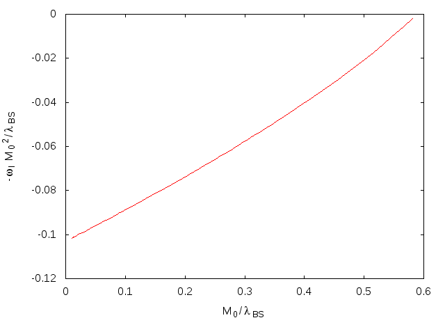
Refer to caption
(a)
Refer to caption
(b)
Figure 3.5: (left) Behavior of the fit parameter τ\tau with respect to the coupling constant λ\lambda. (right) Reproduction of the behavior of −ωI​M02λB​S-\omega_{I}\frac{M_{0}^{2}}{\lambda_{BS}} vs M0λB​S\frac{M_{0}}{\lambda_{BS}} contained in ref. [48], using ωI\omega_{I} obtained from the fit parameter τ\tau. λB​S=8​λ\lambda_{BS}=\sqrt{8\lambda} is the coupling constant used by Blázquez-Salcedo et al. in ref. [48].

3.4 Study of the Apparent Horizon

In this section we want to study the behavior of the apparent horizon.
In spherical symmetry the apparent horizons are defined by the condition (see ref. [62])

∇αR​∇αR=0,\nabla_{\alpha}R\nabla^{\alpha}R=0, (3.58)

where RR is the areal radius of the horizon.
In the metric that we are using the areal radius is a coordinate and the equation for the horizon is given by [62]

gr​r=0.g^{rr}=0. (3.59)

Hence at the second order in ϵ\epsilon we have to solve

1−2​M0r−ϵ2​2​M2r=0.1-\frac{2M_{0}}{r}-\epsilon^{2}\frac{2M_{2}}{r}=0. (3.60)

Since the term M⁡(r,t)M(r,t) is expanded as M⁡(r,t)=M0+ϵ2​M2​(r,t)M(r,t)=M_{0}+\epsilon^{2}M_{2}(r,t), in order for the perturbative expansion to be valid, we imposed the condition

ϵ2​M2<M0.\epsilon^{2}M_{2}<M_{0}. (3.61)

In the stable cases it is sufficient to set a value for ϵ\epsilon such that the condition is valid for every timestep, while in the unstable cases this cannot be done because of the growth of M2M_{2}, and therefore, once set the value of ϵ\epsilon, the equation (3.60) can be solved only for timesteps in which the condition (3.61) is valid. In both cases we used ϵ=0.1\epsilon=0.1.
Moreover, as it can be seen from eq. (3.42), the boundary condition M2​(z0,t)M_{2}(z_{0},t) can be imposed only when the scalar field is null at the numerical inner boundary, and therefore we computed the apparent horizon only for timesteps such that φ1​(z0,t)=0\varphi_{1}(z_{0},t)=0. In order for this condition to be valid for as sufficiently large time, for the following results we used data obtained from simulations on a grid with 13000 points in a region that extends from zM0=−53.26\frac{z}{M_{0}}=-53.26 up to zM0=330.11\frac{z}{M_{0}}=330.11.

3.4.1 Behavior of the Apparent Horizon

The behaviors of the apparent horizon in the cases λM02=0\frac{\lambda}{M_{0}^{2}}=0, λM02=−0.5\frac{\lambda}{M_{0}^{2}}=-0.5 and λM02=0.5\frac{\lambda}{M_{0}^{2}}=0.5 are shown in fig. 3.6.

Refer to caption
(a)
Refer to caption
(b)
Refer to caption
(c)
Figure 3.6: Behavior of the apparent horizon for λM02=0\frac{\lambda}{M_{0}^{2}}=0 (upper left), λM02=−0.5\frac{\lambda}{M_{0}^{2}}=-0.5 (upper right) and λM02=0.5\frac{\lambda}{M_{0}^{2}}=0.5 (lower).

In the stable cases we could solve the eq. (3.60) only for tM0≲40\frac{t}{M_{0}}\lesssim 40 because for later timesteps the condition φ1​(z0,t)=0\varphi_{1}(z_{0},t)=0 does not hold anymore. For λM02=0\frac{\lambda}{M_{0}^{2}}=0 the position of the apparent horizon increases with time and converges to rA​HM0=2.21\frac{r_{AH}}{M_{0}}=2.21, while for λM02=−0.5\frac{\lambda}{M_{0}^{2}}=-0.5 it oscillates before stabilizing at rA​HM0=2.13\frac{r_{AH}}{M_{0}}=2.13.
In the unstable case with λM02=0.5\frac{\lambda}{M_{0}^{2}}=0.5 the apparent horizon could be computed only for tM0≲25\frac{t}{M_{0}}\lesssim 25 in order for the condition (3.61) to be valid. In this case rA​Hr_{AH} initially increases, reaches a maximum at rA​HM0=2.27\frac{r_{AH}}{M_{0}}=2.27 and then decreases converging to r=2​M0r=2M_{0}.

3.4.2 Null Energy Condition in a Perturbative Scheme

In order to understand the behaviors of the apparent horizon that appear in fig. 3.6 we want to check whether the Null Energy Condition (NEC) is satisfied or not. When the condition (3.62) is satisfied the position of the apparent horizon increases, while it could decrease when the NEC is violated [63].
The NEC requires that

Tμ​ν​nμ​nν≥0,T^{\mu\nu}n_{\mu}n_{\nu}\geq 0, (3.62)

for any null vector nμn^{\mu} [27].
Since in the coordinates that we are using the definition of the apparent horizon (3.58) reduces to (3.59), then at rA​Hr_{AH} the vector nμ=(0,1,0,0)n_{\mu}=(0,1,0,0) is null and the NEC reduces to

Tr​r≥0,T^{rr}\geq 0, (3.63)

where the Tr​rT^{rr} is given by

Tr​r=ϵ22​r10​(−6144​λ2​M03​(2​M0−r)​φ1​(r,t)2+CLOSE+64​λ​M0​r4​(2​M0−r)​φ1​(r,t)​((5​M0−3​r)​φ1(1,0)​(r,t)+r⁡(2​M0−r)​φ1(2,0)​(r,t))+OPEN+r7​((64​λ​M0+r3)​φ1(0,1)​(r,t)2+r​(r−2​M0)2​φ1(1,0)​(r,t)2))+𝒪⁡(ϵ3).T^{rr}=\frac{\epsilon^{2}}{2r^{10}}\Biggl(-6144\lambda^{2}M_{0}^{3}(2M_{0}-r)\varphi_{1}(r,t)^{2}+\\ +64\lambda M_{0}r^{4}(2M_{0}-r)\varphi_{1}(r,t)\biggl((5M_{0}-3r)\varphi_{1}^{(1,0)}(r,t)+r(2M_{0}-r)\varphi_{1}^{(2,0)}(r,t)\biggr)+\\ +r^{7}\left(\left(64\lambda M_{0}+r^{3}\right)\varphi_{1}^{(0,1)}(r,t)^{2}+r(r-2M_{0})^{2}\varphi_{1}^{(1,0)}(r,t)^{2}\right)\Biggr)+\mathcal{O}\left(\epsilon^{3}\right). (3.64)

Instead in a generic point of the spacetime we can start from a 4-vector of the form nμ=(nt,1,0,0)n_{\mu}=(n_{t},1,0,0) and impose that it is null:

0=nμ​nμ=gμ​ν​nμ​nν=gt​t​nt2+gr​r.0=n_{\mu}n^{\mu}=g^{\mu\nu}n_{\mu}n_{\nu}=g^{tt}n_{t}^{2}+g^{rr}. (3.65)

Using eq. (3.65) we can write nt2n_{t}^{2} as

nt2=−gr​rgt​t,n_{t}^{2}=-\frac{g^{rr}}{g^{tt}}, (3.66)

and the NEC is given by

Tt​t​nt2+Tr​r=−gr​rgt​t=−gr​r​gt​t​Tt​t+Tr​r==−gr​r​T​tt​+Tr​r=−(1−2​M0r)​T​tt​+Tr​r+𝒪⁡(ϵ4)≥0,T^{tt}n_{t}^{2}+T^{rr}=-\frac{g^{rr}}{g^{tt}}=-g^{rr}g_{tt}T^{tt}+T^{rr}=\\ =-g^{rr}\mathchoice{T^{{{t}\mathchoice{\makebox[3.02084pt][c]{$\displaystyle$}}{\makebox[3.02084pt][c]{$\textstyle$}}{\makebox[1.76944pt][c]{$\scriptstyle$}}{\makebox[1.26389pt][c]{$\scriptscriptstyle$}}}}_{{\mathchoice{\makebox[3.02084pt][c]{$\displaystyle$}}{\makebox[3.02084pt][c]{$\textstyle$}}{\makebox[1.76944pt][c]{$\scriptstyle$}}{\makebox[1.26389pt][c]{$\scriptscriptstyle$}}{t}}}}{T^{{{t}\mathchoice{\makebox[3.02084pt][c]{$\displaystyle$}}{\makebox[3.02084pt][c]{$\textstyle$}}{\makebox[1.76944pt][c]{$\scriptstyle$}}{\makebox[1.26389pt][c]{$\scriptscriptstyle$}}}}_{{\mathchoice{\makebox[3.02084pt][c]{$\displaystyle$}}{\makebox[3.02084pt][c]{$\textstyle$}}{\makebox[1.76944pt][c]{$\scriptstyle$}}{\makebox[1.26389pt][c]{$\scriptscriptstyle$}}{t}}}}{T^{{{t}\mathchoice{\makebox[3.02084pt][c]{$\displaystyle$}}{\makebox[3.02084pt][c]{$\textstyle$}}{\makebox[1.76944pt][c]{$\scriptstyle$}}{\makebox[1.26389pt][c]{$\scriptscriptstyle$}}}}_{{\mathchoice{\makebox[3.02084pt][c]{$\displaystyle$}}{\makebox[3.02084pt][c]{$\textstyle$}}{\makebox[1.76944pt][c]{$\scriptstyle$}}{\makebox[1.26389pt][c]{$\scriptscriptstyle$}}{t}}}}{T^{{{t}\mathchoice{\makebox[3.02084pt][c]{$\displaystyle$}}{\makebox[3.02084pt][c]{$\textstyle$}}{\makebox[1.76944pt][c]{$\scriptstyle$}}{\makebox[1.26389pt][c]{$\scriptscriptstyle$}}}}_{{\mathchoice{\makebox[3.02084pt][c]{$\displaystyle$}}{\makebox[3.02084pt][c]{$\textstyle$}}{\makebox[1.76944pt][c]{$\scriptstyle$}}{\makebox[1.26389pt][c]{$\scriptscriptstyle$}}{t}}}}+T^{rr}=-\biggl(1-\frac{2M_{0}}{r}\biggr)\mathchoice{T^{{{t}\mathchoice{\makebox[3.02084pt][c]{$\displaystyle$}}{\makebox[3.02084pt][c]{$\textstyle$}}{\makebox[1.76944pt][c]{$\scriptstyle$}}{\makebox[1.26389pt][c]{$\scriptscriptstyle$}}}}_{{\mathchoice{\makebox[3.02084pt][c]{$\displaystyle$}}{\makebox[3.02084pt][c]{$\textstyle$}}{\makebox[1.76944pt][c]{$\scriptstyle$}}{\makebox[1.26389pt][c]{$\scriptscriptstyle$}}{t}}}}{T^{{{t}\mathchoice{\makebox[3.02084pt][c]{$\displaystyle$}}{\makebox[3.02084pt][c]{$\textstyle$}}{\makebox[1.76944pt][c]{$\scriptstyle$}}{\makebox[1.26389pt][c]{$\scriptscriptstyle$}}}}_{{\mathchoice{\makebox[3.02084pt][c]{$\displaystyle$}}{\makebox[3.02084pt][c]{$\textstyle$}}{\makebox[1.76944pt][c]{$\scriptstyle$}}{\makebox[1.26389pt][c]{$\scriptscriptstyle$}}{t}}}}{T^{{{t}\mathchoice{\makebox[3.02084pt][c]{$\displaystyle$}}{\makebox[3.02084pt][c]{$\textstyle$}}{\makebox[1.76944pt][c]{$\scriptstyle$}}{\makebox[1.26389pt][c]{$\scriptscriptstyle$}}}}_{{\mathchoice{\makebox[3.02084pt][c]{$\displaystyle$}}{\makebox[3.02084pt][c]{$\textstyle$}}{\makebox[1.76944pt][c]{$\scriptstyle$}}{\makebox[1.26389pt][c]{$\scriptscriptstyle$}}{t}}}}{T^{{{t}\mathchoice{\makebox[3.02084pt][c]{$\displaystyle$}}{\makebox[3.02084pt][c]{$\textstyle$}}{\makebox[1.76944pt][c]{$\scriptstyle$}}{\makebox[1.26389pt][c]{$\scriptscriptstyle$}}}}_{{\mathchoice{\makebox[3.02084pt][c]{$\displaystyle$}}{\makebox[3.02084pt][c]{$\textstyle$}}{\makebox[1.76944pt][c]{$\scriptstyle$}}{\makebox[1.26389pt][c]{$\scriptscriptstyle$}}{t}}}}+T^{rr}+\mathcal{O}(\epsilon^{4})\geq 0, (3.67)

where

Tt​​t=ϵ22​r5[r6​φ1(0,1)​(r,t)22​M0−r−r(r−2M0)(64λM0+r3)φ1(1,0)(r,t)2++64λM0φ1(r,t)((r−3M0)φ1(1,0)(r,t)+r(2M0−r)φ1(2,0)(r,t))]+𝒪(ϵ3).\mathchoice{T^{{{t}\mathchoice{\makebox[3.02084pt][c]{$\displaystyle$}}{\makebox[3.02084pt][c]{$\textstyle$}}{\makebox[1.76944pt][c]{$\scriptstyle$}}{\makebox[1.26389pt][c]{$\scriptscriptstyle$}}}}_{{\mathchoice{\makebox[3.02084pt][c]{$\displaystyle$}}{\makebox[3.02084pt][c]{$\textstyle$}}{\makebox[1.76944pt][c]{$\scriptstyle$}}{\makebox[1.26389pt][c]{$\scriptscriptstyle$}}{t}}}}{T^{{{t}\mathchoice{\makebox[3.02084pt][c]{$\displaystyle$}}{\makebox[3.02084pt][c]{$\textstyle$}}{\makebox[1.76944pt][c]{$\scriptstyle$}}{\makebox[1.26389pt][c]{$\scriptscriptstyle$}}}}_{{\mathchoice{\makebox[3.02084pt][c]{$\displaystyle$}}{\makebox[3.02084pt][c]{$\textstyle$}}{\makebox[1.76944pt][c]{$\scriptstyle$}}{\makebox[1.26389pt][c]{$\scriptscriptstyle$}}{t}}}}{T^{{{t}\mathchoice{\makebox[3.02084pt][c]{$\displaystyle$}}{\makebox[3.02084pt][c]{$\textstyle$}}{\makebox[1.76944pt][c]{$\scriptstyle$}}{\makebox[1.26389pt][c]{$\scriptscriptstyle$}}}}_{{\mathchoice{\makebox[3.02084pt][c]{$\displaystyle$}}{\makebox[3.02084pt][c]{$\textstyle$}}{\makebox[1.76944pt][c]{$\scriptstyle$}}{\makebox[1.26389pt][c]{$\scriptscriptstyle$}}{t}}}}{T^{{{t}\mathchoice{\makebox[3.02084pt][c]{$\displaystyle$}}{\makebox[3.02084pt][c]{$\textstyle$}}{\makebox[1.76944pt][c]{$\scriptstyle$}}{\makebox[1.26389pt][c]{$\scriptscriptstyle$}}}}_{{\mathchoice{\makebox[3.02084pt][c]{$\displaystyle$}}{\makebox[3.02084pt][c]{$\textstyle$}}{\makebox[1.76944pt][c]{$\scriptstyle$}}{\makebox[1.26389pt][c]{$\scriptscriptstyle$}}{t}}}}=\frac{\epsilon^{2}}{2r^{5}}\biggl[\frac{r^{6}\varphi_{1}^{(0,1)}(r,t)^{2}}{2M_{0}-r}-r\left(r-2M_{0}\right)\left(64\lambda M_{0}+r^{3}\right)\varphi_{1}^{(1,0)}(r,t)^{2}+\\ +64\lambda M_{0}\varphi_{1}(r,t)\left(\left(r-3M_{0}\right)\varphi_{1}^{(1,0)}(r,t)+r\left(2M_{0}-r\right)\varphi_{1}^{(2,0)}(r,t)\right)\biggr]+\mathcal{O}\left(\epsilon^{3}\right). (3.68)

In eq. (3.67) we used the fact that Tt=t𝒪(ϵ2)\mathchoice{T^{{{t}}}_{{\mathchoice{\makebox[3.02084pt][c]{$\displaystyle$}}{\makebox[3.02084pt][c]{$\textstyle$}}{\makebox[1.76944pt][c]{$\scriptstyle$}}{\makebox[1.26389pt][c]{$\scriptscriptstyle$}}}}}{T^{{{t}}}_{{\mathchoice{\makebox[3.02084pt][c]{$\displaystyle$}}{\makebox[3.02084pt][c]{$\textstyle$}}{\makebox[1.76944pt][c]{$\scriptstyle$}}{\makebox[1.26389pt][c]{$\scriptscriptstyle$}}}}}{T^{{{t}}}_{{\mathchoice{\makebox[3.02084pt][c]{$\displaystyle$}}{\makebox[3.02084pt][c]{$\textstyle$}}{\makebox[1.76944pt][c]{$\scriptstyle$}}{\makebox[1.26389pt][c]{$\scriptscriptstyle$}}}}}{T^{{{t}}}_{{\mathchoice{\makebox[3.02084pt][c]{$\displaystyle$}}{\makebox[3.02084pt][c]{$\textstyle$}}{\makebox[1.76944pt][c]{$\scriptstyle$}}{\makebox[1.26389pt][c]{$\scriptscriptstyle$}}}}}{{}_{t}}=\mathcal{O}(\epsilon^{2}).
In principle at the apparent horizon (3.63) and (3.67) should coincide, since

(1−2​M0r)​T​tt​=ϵ2​2​M2r​T​tt​=𝒪⁡(ϵ4).\biggl(1-\frac{2M_{0}}{r}\biggr)\mathchoice{T^{{{t}\mathchoice{\makebox[3.02084pt][c]{$\displaystyle$}}{\makebox[3.02084pt][c]{$\textstyle$}}{\makebox[1.76944pt][c]{$\scriptstyle$}}{\makebox[1.26389pt][c]{$\scriptscriptstyle$}}}}_{{\mathchoice{\makebox[3.02084pt][c]{$\displaystyle$}}{\makebox[3.02084pt][c]{$\textstyle$}}{\makebox[1.76944pt][c]{$\scriptstyle$}}{\makebox[1.26389pt][c]{$\scriptscriptstyle$}}{t}}}}{T^{{{t}\mathchoice{\makebox[3.02084pt][c]{$\displaystyle$}}{\makebox[3.02084pt][c]{$\textstyle$}}{\makebox[1.76944pt][c]{$\scriptstyle$}}{\makebox[1.26389pt][c]{$\scriptscriptstyle$}}}}_{{\mathchoice{\makebox[3.02084pt][c]{$\displaystyle$}}{\makebox[3.02084pt][c]{$\textstyle$}}{\makebox[1.76944pt][c]{$\scriptstyle$}}{\makebox[1.26389pt][c]{$\scriptscriptstyle$}}{t}}}}{T^{{{t}\mathchoice{\makebox[3.02084pt][c]{$\displaystyle$}}{\makebox[3.02084pt][c]{$\textstyle$}}{\makebox[1.76944pt][c]{$\scriptstyle$}}{\makebox[1.26389pt][c]{$\scriptscriptstyle$}}}}_{{\mathchoice{\makebox[3.02084pt][c]{$\displaystyle$}}{\makebox[3.02084pt][c]{$\textstyle$}}{\makebox[1.76944pt][c]{$\scriptstyle$}}{\makebox[1.26389pt][c]{$\scriptscriptstyle$}}{t}}}}{T^{{{t}\mathchoice{\makebox[3.02084pt][c]{$\displaystyle$}}{\makebox[3.02084pt][c]{$\textstyle$}}{\makebox[1.76944pt][c]{$\scriptstyle$}}{\makebox[1.26389pt][c]{$\scriptscriptstyle$}}}}_{{\mathchoice{\makebox[3.02084pt][c]{$\displaystyle$}}{\makebox[3.02084pt][c]{$\textstyle$}}{\makebox[1.76944pt][c]{$\scriptstyle$}}{\makebox[1.26389pt][c]{$\scriptscriptstyle$}}{t}}}}=\epsilon^{2}\frac{2M_{2}}{r}\mathchoice{T^{{{t}\mathchoice{\makebox[3.02084pt][c]{$\displaystyle$}}{\makebox[3.02084pt][c]{$\textstyle$}}{\makebox[1.76944pt][c]{$\scriptstyle$}}{\makebox[1.26389pt][c]{$\scriptscriptstyle$}}}}_{{\mathchoice{\makebox[3.02084pt][c]{$\displaystyle$}}{\makebox[3.02084pt][c]{$\textstyle$}}{\makebox[1.76944pt][c]{$\scriptstyle$}}{\makebox[1.26389pt][c]{$\scriptscriptstyle$}}{t}}}}{T^{{{t}\mathchoice{\makebox[3.02084pt][c]{$\displaystyle$}}{\makebox[3.02084pt][c]{$\textstyle$}}{\makebox[1.76944pt][c]{$\scriptstyle$}}{\makebox[1.26389pt][c]{$\scriptscriptstyle$}}}}_{{\mathchoice{\makebox[3.02084pt][c]{$\displaystyle$}}{\makebox[3.02084pt][c]{$\textstyle$}}{\makebox[1.76944pt][c]{$\scriptstyle$}}{\makebox[1.26389pt][c]{$\scriptscriptstyle$}}{t}}}}{T^{{{t}\mathchoice{\makebox[3.02084pt][c]{$\displaystyle$}}{\makebox[3.02084pt][c]{$\textstyle$}}{\makebox[1.76944pt][c]{$\scriptstyle$}}{\makebox[1.26389pt][c]{$\scriptscriptstyle$}}}}_{{\mathchoice{\makebox[3.02084pt][c]{$\displaystyle$}}{\makebox[3.02084pt][c]{$\textstyle$}}{\makebox[1.76944pt][c]{$\scriptstyle$}}{\makebox[1.26389pt][c]{$\scriptscriptstyle$}}{t}}}}{T^{{{t}\mathchoice{\makebox[3.02084pt][c]{$\displaystyle$}}{\makebox[3.02084pt][c]{$\textstyle$}}{\makebox[1.76944pt][c]{$\scriptstyle$}}{\makebox[1.26389pt][c]{$\scriptscriptstyle$}}}}_{{\mathchoice{\makebox[3.02084pt][c]{$\displaystyle$}}{\makebox[3.02084pt][c]{$\textstyle$}}{\makebox[1.76944pt][c]{$\scriptstyle$}}{\makebox[1.26389pt][c]{$\scriptscriptstyle$}}{t}}}}=\mathcal{O}(\epsilon^{4}). (3.69)

However in numerical computations we found a notable difference between the two expression of the NEC at the apparent horizon.
In order to understand this aspect we checked that the perturbative expansion of the apparent horizon behaves correctly. In our scheme the position of the apparent horizon can be written as

rA​H=2​M0​(1+ϵ2​M2M0).r_{AH}=2M_{0}\biggl(1+\epsilon^{2}\frac{M_{2}}{M_{0}}\biggr). (3.70)

We verified numerically that the term rA​H−2​M0r_{AH}-2M_{0} scales quadratically in ϵ\epsilon obtaining the results shown in fig. 3.7. Therefore we conclude that at least in the stable cases rA​Hr_{AH} behaves correctly in perturbation theory.

Refer to caption
(a)
Refer to caption
(b)
Refer to caption
(c)
Figure 3.7: Scaling of rA​H−2​M0r_{AH}-2M_{0} renormalized by M0M_{0} in the cases λM02=0\frac{\lambda}{M_{0}^{2}}=0 (upper left), λM02=−0.5\frac{\lambda}{M_{0}^{2}}=-0.5 (upper right) and λM02=0.5\frac{\lambda}{M_{0}^{2}}=0.5 (lower). The points in the plots represent the values of rA​HM0−2\frac{r_{AH}}{M_{0}}-2 obtained from the computation of the apparent horizon using three different values of ϵ\epsilon, while the solid lines are obtained by rescaling quadratically in ϵ\epsilon the values with the same color. In particular, the red solid line represents the values of rA​HM0−2\frac{r_{AH}}{M_{0}}-2 computed with ϵ=0.07\epsilon=0.07 and rescaled by 0.120.072\frac{0.1^{2}}{0.07^{2}} while the blue solid line is obtained from a computation of the horizon with ϵ=0.05\epsilon=0.05 with a rescaling of 0.0720.052\frac{0.07^{2}}{0.05^{2}}.

From the numerical computations of T​tt​\mathchoice{T^{{{t}\mathchoice{\makebox[3.02084pt][c]{$\displaystyle$}}{\makebox[3.02084pt][c]{$\textstyle$}}{\makebox[1.76944pt][c]{$\scriptstyle$}}{\makebox[1.26389pt][c]{$\scriptscriptstyle$}}}}_{{\mathchoice{\makebox[3.02084pt][c]{$\displaystyle$}}{\makebox[3.02084pt][c]{$\textstyle$}}{\makebox[1.76944pt][c]{$\scriptstyle$}}{\makebox[1.26389pt][c]{$\scriptscriptstyle$}}{t}}}}{T^{{{t}\mathchoice{\makebox[3.02084pt][c]{$\displaystyle$}}{\makebox[3.02084pt][c]{$\textstyle$}}{\makebox[1.76944pt][c]{$\scriptstyle$}}{\makebox[1.26389pt][c]{$\scriptscriptstyle$}}}}_{{\mathchoice{\makebox[3.02084pt][c]{$\displaystyle$}}{\makebox[3.02084pt][c]{$\textstyle$}}{\makebox[1.76944pt][c]{$\scriptstyle$}}{\makebox[1.26389pt][c]{$\scriptscriptstyle$}}{t}}}}{T^{{{t}\mathchoice{\makebox[3.02084pt][c]{$\displaystyle$}}{\makebox[3.02084pt][c]{$\textstyle$}}{\makebox[1.76944pt][c]{$\scriptstyle$}}{\makebox[1.26389pt][c]{$\scriptscriptstyle$}}}}_{{\mathchoice{\makebox[3.02084pt][c]{$\displaystyle$}}{\makebox[3.02084pt][c]{$\textstyle$}}{\makebox[1.76944pt][c]{$\scriptstyle$}}{\makebox[1.26389pt][c]{$\scriptscriptstyle$}}{t}}}}{T^{{{t}\mathchoice{\makebox[3.02084pt][c]{$\displaystyle$}}{\makebox[3.02084pt][c]{$\textstyle$}}{\makebox[1.76944pt][c]{$\scriptstyle$}}{\makebox[1.26389pt][c]{$\scriptscriptstyle$}}}}_{{\mathchoice{\makebox[3.02084pt][c]{$\displaystyle$}}{\makebox[3.02084pt][c]{$\textstyle$}}{\makebox[1.76944pt][c]{$\scriptstyle$}}{\makebox[1.26389pt][c]{$\scriptscriptstyle$}}{t}}}} we found that at the apparent horizon it does not scale with ϵ2\epsilon^{2}. This behavior is related to the fact that

T​tt​=ϵ22​r​φ1(0,1)​(r,t)22​M0−r+…,\mathchoice{T^{{{t}\mathchoice{\makebox[3.02084pt][c]{$\displaystyle$}}{\makebox[3.02084pt][c]{$\textstyle$}}{\makebox[1.76944pt][c]{$\scriptstyle$}}{\makebox[1.26389pt][c]{$\scriptscriptstyle$}}}}_{{\mathchoice{\makebox[3.02084pt][c]{$\displaystyle$}}{\makebox[3.02084pt][c]{$\textstyle$}}{\makebox[1.76944pt][c]{$\scriptstyle$}}{\makebox[1.26389pt][c]{$\scriptscriptstyle$}}{t}}}}{T^{{{t}\mathchoice{\makebox[3.02084pt][c]{$\displaystyle$}}{\makebox[3.02084pt][c]{$\textstyle$}}{\makebox[1.76944pt][c]{$\scriptstyle$}}{\makebox[1.26389pt][c]{$\scriptscriptstyle$}}}}_{{\mathchoice{\makebox[3.02084pt][c]{$\displaystyle$}}{\makebox[3.02084pt][c]{$\textstyle$}}{\makebox[1.76944pt][c]{$\scriptstyle$}}{\makebox[1.26389pt][c]{$\scriptscriptstyle$}}{t}}}}{T^{{{t}\mathchoice{\makebox[3.02084pt][c]{$\displaystyle$}}{\makebox[3.02084pt][c]{$\textstyle$}}{\makebox[1.76944pt][c]{$\scriptstyle$}}{\makebox[1.26389pt][c]{$\scriptscriptstyle$}}}}_{{\mathchoice{\makebox[3.02084pt][c]{$\displaystyle$}}{\makebox[3.02084pt][c]{$\textstyle$}}{\makebox[1.76944pt][c]{$\scriptstyle$}}{\makebox[1.26389pt][c]{$\scriptscriptstyle$}}{t}}}}{T^{{{t}\mathchoice{\makebox[3.02084pt][c]{$\displaystyle$}}{\makebox[3.02084pt][c]{$\textstyle$}}{\makebox[1.76944pt][c]{$\scriptstyle$}}{\makebox[1.26389pt][c]{$\scriptscriptstyle$}}}}_{{\mathchoice{\makebox[3.02084pt][c]{$\displaystyle$}}{\makebox[3.02084pt][c]{$\textstyle$}}{\makebox[1.76944pt][c]{$\scriptstyle$}}{\makebox[1.26389pt][c]{$\scriptscriptstyle$}}{t}}}}=\frac{\epsilon^{2}}{2}\frac{r\varphi_{1}^{(0,1)}(r,t)^{2}}{2M_{0}-r}+\dots\quad, (3.71)

and since rA​H−2​M0=𝒪⁡(ϵ2)r_{AH}-2M_{0}=\mathcal{O}(\epsilon^{2}), then at the apparent horizon T​tt​=𝒪⁡(1)\mathchoice{T^{{{t}\mathchoice{\makebox[3.02084pt][c]{$\displaystyle$}}{\makebox[3.02084pt][c]{$\textstyle$}}{\makebox[1.76944pt][c]{$\scriptstyle$}}{\makebox[1.26389pt][c]{$\scriptscriptstyle$}}}}_{{\mathchoice{\makebox[3.02084pt][c]{$\displaystyle$}}{\makebox[3.02084pt][c]{$\textstyle$}}{\makebox[1.76944pt][c]{$\scriptstyle$}}{\makebox[1.26389pt][c]{$\scriptscriptstyle$}}{t}}}}{T^{{{t}\mathchoice{\makebox[3.02084pt][c]{$\displaystyle$}}{\makebox[3.02084pt][c]{$\textstyle$}}{\makebox[1.76944pt][c]{$\scriptstyle$}}{\makebox[1.26389pt][c]{$\scriptscriptstyle$}}}}_{{\mathchoice{\makebox[3.02084pt][c]{$\displaystyle$}}{\makebox[3.02084pt][c]{$\textstyle$}}{\makebox[1.76944pt][c]{$\scriptstyle$}}{\makebox[1.26389pt][c]{$\scriptscriptstyle$}}{t}}}}{T^{{{t}\mathchoice{\makebox[3.02084pt][c]{$\displaystyle$}}{\makebox[3.02084pt][c]{$\textstyle$}}{\makebox[1.76944pt][c]{$\scriptstyle$}}{\makebox[1.26389pt][c]{$\scriptscriptstyle$}}}}_{{\mathchoice{\makebox[3.02084pt][c]{$\displaystyle$}}{\makebox[3.02084pt][c]{$\textstyle$}}{\makebox[1.76944pt][c]{$\scriptstyle$}}{\makebox[1.26389pt][c]{$\scriptscriptstyle$}}{t}}}}{T^{{{t}\mathchoice{\makebox[3.02084pt][c]{$\displaystyle$}}{\makebox[3.02084pt][c]{$\textstyle$}}{\makebox[1.76944pt][c]{$\scriptstyle$}}{\makebox[1.26389pt][c]{$\scriptscriptstyle$}}}}_{{\mathchoice{\makebox[3.02084pt][c]{$\displaystyle$}}{\makebox[3.02084pt][c]{$\textstyle$}}{\makebox[1.76944pt][c]{$\scriptstyle$}}{\makebox[1.26389pt][c]{$\scriptscriptstyle$}}{t}}}}=\mathcal{O}(1) and therefore (1−2​M0r)​T​tt​\Bigl(1-\frac{2M_{0}}{r}\Bigr)\mathchoice{T^{{{t}\mathchoice{\makebox[3.02084pt][c]{$\displaystyle$}}{\makebox[3.02084pt][c]{$\textstyle$}}{\makebox[1.76944pt][c]{$\scriptstyle$}}{\makebox[1.26389pt][c]{$\scriptscriptstyle$}}}}_{{\mathchoice{\makebox[3.02084pt][c]{$\displaystyle$}}{\makebox[3.02084pt][c]{$\textstyle$}}{\makebox[1.76944pt][c]{$\scriptstyle$}}{\makebox[1.26389pt][c]{$\scriptscriptstyle$}}{t}}}}{T^{{{t}\mathchoice{\makebox[3.02084pt][c]{$\displaystyle$}}{\makebox[3.02084pt][c]{$\textstyle$}}{\makebox[1.76944pt][c]{$\scriptstyle$}}{\makebox[1.26389pt][c]{$\scriptscriptstyle$}}}}_{{\mathchoice{\makebox[3.02084pt][c]{$\displaystyle$}}{\makebox[3.02084pt][c]{$\textstyle$}}{\makebox[1.76944pt][c]{$\scriptstyle$}}{\makebox[1.26389pt][c]{$\scriptscriptstyle$}}{t}}}}{T^{{{t}\mathchoice{\makebox[3.02084pt][c]{$\displaystyle$}}{\makebox[3.02084pt][c]{$\textstyle$}}{\makebox[1.76944pt][c]{$\scriptstyle$}}{\makebox[1.26389pt][c]{$\scriptscriptstyle$}}}}_{{\mathchoice{\makebox[3.02084pt][c]{$\displaystyle$}}{\makebox[3.02084pt][c]{$\textstyle$}}{\makebox[1.76944pt][c]{$\scriptstyle$}}{\makebox[1.26389pt][c]{$\scriptscriptstyle$}}{t}}}}{T^{{{t}\mathchoice{\makebox[3.02084pt][c]{$\displaystyle$}}{\makebox[3.02084pt][c]{$\textstyle$}}{\makebox[1.76944pt][c]{$\scriptstyle$}}{\makebox[1.26389pt][c]{$\scriptscriptstyle$}}}}_{{\mathchoice{\makebox[3.02084pt][c]{$\displaystyle$}}{\makebox[3.02084pt][c]{$\textstyle$}}{\makebox[1.76944pt][c]{$\scriptstyle$}}{\makebox[1.26389pt][c]{$\scriptscriptstyle$}}{t}}}} scales with ϵ2\epsilon^{2}.
The analysis we reported in this section has highlighted a criticality in studying the apparent horizon from a perturbative point of view. In fact in the stable cases, while rA​Hr_{AH} shows the correct behavior in perturbation theory, the NEC cannot be computed with an expansion in ϵ\epsilon, since near the apparent horizon the terms in ϵ4\epsilon^{4} are not negligible with respect to the terms in ϵ2\epsilon^{2}.
This critical issue can be due to the fact that we are using Schwarzschild coordinates, which are not regular. A different choice of coordinates may allow to study the behavior of the apparent horizon in a perturbative framework.
However, it is possible to perform a perturbative analysis in Schwarzschild coordinates for timesteps in which the apparent horizon is absent, since in this case T​tt​\mathchoice{T^{{{t}\mathchoice{\makebox[3.02084pt][c]{$\displaystyle$}}{\makebox[3.02084pt][c]{$\textstyle$}}{\makebox[1.76944pt][c]{$\scriptstyle$}}{\makebox[1.26389pt][c]{$\scriptscriptstyle$}}}}_{{\mathchoice{\makebox[3.02084pt][c]{$\displaystyle$}}{\makebox[3.02084pt][c]{$\textstyle$}}{\makebox[1.76944pt][c]{$\scriptstyle$}}{\makebox[1.26389pt][c]{$\scriptscriptstyle$}}{t}}}}{T^{{{t}\mathchoice{\makebox[3.02084pt][c]{$\displaystyle$}}{\makebox[3.02084pt][c]{$\textstyle$}}{\makebox[1.76944pt][c]{$\scriptstyle$}}{\makebox[1.26389pt][c]{$\scriptscriptstyle$}}}}_{{\mathchoice{\makebox[3.02084pt][c]{$\displaystyle$}}{\makebox[3.02084pt][c]{$\textstyle$}}{\makebox[1.76944pt][c]{$\scriptstyle$}}{\makebox[1.26389pt][c]{$\scriptscriptstyle$}}{t}}}}{T^{{{t}\mathchoice{\makebox[3.02084pt][c]{$\displaystyle$}}{\makebox[3.02084pt][c]{$\textstyle$}}{\makebox[1.76944pt][c]{$\scriptstyle$}}{\makebox[1.26389pt][c]{$\scriptscriptstyle$}}}}_{{\mathchoice{\makebox[3.02084pt][c]{$\displaystyle$}}{\makebox[3.02084pt][c]{$\textstyle$}}{\makebox[1.76944pt][c]{$\scriptstyle$}}{\makebox[1.26389pt][c]{$\scriptscriptstyle$}}{t}}}}{T^{{{t}\mathchoice{\makebox[3.02084pt][c]{$\displaystyle$}}{\makebox[3.02084pt][c]{$\textstyle$}}{\makebox[1.76944pt][c]{$\scriptstyle$}}{\makebox[1.26389pt][c]{$\scriptscriptstyle$}}}}_{{\mathchoice{\makebox[3.02084pt][c]{$\displaystyle$}}{\makebox[3.02084pt][c]{$\textstyle$}}{\makebox[1.76944pt][c]{$\scriptstyle$}}{\makebox[1.26389pt][c]{$\scriptscriptstyle$}}{t}}}} scales correctly. Moreover, decreasing the value of ϵ\epsilon, the energy of the field decreases, and the process of formation of the apparent horizon is slower (cf. fig. 3.7, the curves corresponding to smaller ϵ\epsilon start later). In this way it is possible to perform analysis in larger intervals of time, by setting sufficiently small values of ϵ\epsilon.

Chapter 4 Schwarzschild BHs in EsGB Gravity with Quartic Coupling

In this chapter we are going to analyze the stability of a Schwarschild BH in EsGB theory using a quartic coupling function F⁡[ϕ]=λ​ϕ2+γ​ϕ4F[\phi]=\lambda\phi^{2}+\gamma\phi^{4}. We will start by describing the perturbative scheme we are going to use in this case, then we will derive the field equations in 1+1 variables at the first order around the Schwarzschild solution, and we will study the stability of the BH, with a focus on the case γλ<0\frac{\gamma}{\lambda}<0.

4.1 Quartic EsGB Gravity and Perturbative Scheme

EsGB gravity with quartic coupling function is particularly interesting since the Euler-Lagrange equation for the scalar field has a nonlinear term that can quench the tachyonic instability leading to the appearance of stable scalarized solutions [49]. However this cannot happen in a perturbative scheme where the scalar field is expanded around the Schwarzschild solution, since at the second order in ϵ\epsilon the quartic term does not contribute in the equations. Therefore, since we are interested in treating the quadratic and the quartic term in the scalar field at the same order in perturbation theory, we decided to perform an expansion of the gravitational constant GG around 0.

4.1.1 Action and Field Equations

In order to use this perturbative scheme we rewrite the action as

S=12​∫Ωd4​x​−g​{R−G​(∇ϕ)2+2​G​F​[ϕ]​𝒢}.S=\frac{1}{2}\int_{\Omega}d^{4}x\sqrt{-g}\biggl\{R-G(\nabla\phi)^{2}+2GF[\phi]\mathcal{G}\biggr\}. (4.1)

In eq. (4.1) and in the rest of the computations we have absorbed a factor 8​π8\pi in the Newton’s constant.
The field equations obtained from the action (4.1) are

E(ϕ):=G​∇μ​∇μϕ+G​δ​F​[ϕ]δ​ϕ​𝒢=0,E^{(\phi)}:=G\nabla_{\mu}\nabla^{\mu}\phi+G\frac{\delta F[\phi]}{\delta\phi}\mathcal{G}=0, (4.2)
Eμ​ν(g):=Rμ​ν−12​gμ​ν​R+G​12​(∇ϕ)2​gμ​ν−G⁡(∇μϕ)​(∇νϕ)++2​G​(∇γ∇α​F​[ϕ])​δα​β​ρ​σγ​δ​κ​λ​R​κ​λρ​σ​​δμβ​gν​δ=0.E^{(g)}_{\mu\nu}:=R_{\mu\nu}-\frac{1}{2}g_{\mu\nu}R+G\frac{1}{2}\bigl(\nabla\phi\bigr)^{2}g_{\mu\nu}-G\bigl(\nabla_{\mu}\phi\bigr)\bigl(\nabla_{\nu}\phi\bigr)+\\ +2G\Bigl(\nabla_{\gamma}\nabla^{\alpha}F[\phi]\Bigr)\delta^{\gamma\delta\kappa\lambda}_{\alpha\beta\rho\sigma}\mathchoice{R^{{{\rho\sigma}\mathchoice{\makebox[9.42482pt][c]{$\displaystyle$}}{\makebox[9.42482pt][c]{$\textstyle$}}{\makebox[5.68152pt][c]{$\scriptstyle$}}{\makebox[4.05823pt][c]{$\scriptscriptstyle$}}}}_{{\mathchoice{\makebox[8.78293pt][c]{$\displaystyle$}}{\makebox[8.78293pt][c]{$\textstyle$}}{\makebox[5.3333pt][c]{$\scriptstyle$}}{\makebox[3.80948pt][c]{$\scriptscriptstyle$}}{\kappa\lambda}}}}{R^{{{\rho\sigma}\mathchoice{\makebox[9.42482pt][c]{$\displaystyle$}}{\makebox[9.42482pt][c]{$\textstyle$}}{\makebox[5.68152pt][c]{$\scriptstyle$}}{\makebox[4.05823pt][c]{$\scriptscriptstyle$}}}}_{{\mathchoice{\makebox[8.78293pt][c]{$\displaystyle$}}{\makebox[8.78293pt][c]{$\textstyle$}}{\makebox[5.3333pt][c]{$\scriptstyle$}}{\makebox[3.80948pt][c]{$\scriptscriptstyle$}}{\kappa\lambda}}}}{R^{{{\rho\sigma}\mathchoice{\makebox[9.42482pt][c]{$\displaystyle$}}{\makebox[9.42482pt][c]{$\textstyle$}}{\makebox[5.68152pt][c]{$\scriptstyle$}}{\makebox[4.05823pt][c]{$\scriptscriptstyle$}}}}_{{\mathchoice{\makebox[8.78293pt][c]{$\displaystyle$}}{\makebox[8.78293pt][c]{$\textstyle$}}{\makebox[5.3333pt][c]{$\scriptstyle$}}{\makebox[3.80948pt][c]{$\scriptscriptstyle$}}{\kappa\lambda}}}}{R^{{{\rho\sigma}\mathchoice{\makebox[9.42482pt][c]{$\displaystyle$}}{\makebox[9.42482pt][c]{$\textstyle$}}{\makebox[5.68152pt][c]{$\scriptstyle$}}{\makebox[4.05823pt][c]{$\scriptscriptstyle$}}}}_{{\mathchoice{\makebox[8.78293pt][c]{$\displaystyle$}}{\makebox[8.78293pt][c]{$\textstyle$}}{\makebox[5.3333pt][c]{$\scriptstyle$}}{\makebox[3.80948pt][c]{$\scriptscriptstyle$}}{\kappa\lambda}}}}\delta^{\beta}_{\mu}g_{\nu\delta}=0. (4.3)

The equations for the gravitational field Eμ​ν(g)E^{(g)}_{\mu\nu} can be can be rewritten as

Gμ​ν=G​Tμ​ν,G_{\mu\nu}=GT_{\mu\nu}, (4.4)

where Gμ​νG_{\mu\nu} is the Einstein tensor, and the stress-energy tensor Tμ​νT_{\mu\nu} has the same expression as in eq. (3.4)

Tμ​ν=−12​(∇ϕ)2​gμ​ν+(∇μϕ)​(∇νϕ)−2​(∇γ∇α​F​[ϕ])​δα​β​ρ​σγ​δ​κ​λ​R​κ​λρ​σ​​δμβ​gν​δ.\mathchoice{T^{{\mathchoice{\makebox[8.8716pt][c]{$\displaystyle$}}{\makebox[8.8716pt][c]{$\textstyle$}}{\makebox[5.373pt][c]{$\scriptstyle$}}{\makebox[3.83784pt][c]{$\scriptscriptstyle$}}}}_{{{\mu\nu}}}}{T^{{\mathchoice{\makebox[8.8716pt][c]{$\displaystyle$}}{\makebox[8.8716pt][c]{$\textstyle$}}{\makebox[5.373pt][c]{$\scriptstyle$}}{\makebox[3.83784pt][c]{$\scriptscriptstyle$}}}}_{{{\mu\nu}}}}{T^{{\mathchoice{\makebox[8.8716pt][c]{$\displaystyle$}}{\makebox[8.8716pt][c]{$\textstyle$}}{\makebox[5.373pt][c]{$\scriptstyle$}}{\makebox[3.83784pt][c]{$\scriptscriptstyle$}}}}_{{{\mu\nu}}}}{T^{{\mathchoice{\makebox[8.8716pt][c]{$\displaystyle$}}{\makebox[8.8716pt][c]{$\textstyle$}}{\makebox[5.373pt][c]{$\scriptstyle$}}{\makebox[3.83784pt][c]{$\scriptscriptstyle$}}}}_{{{\mu\nu}}}}=-\frac{1}{2}\bigl(\nabla\phi\bigr)^{2}g_{\mu\nu}+\bigl(\nabla_{\mu}\phi\bigr)\bigl(\nabla_{\nu}\phi\bigr)-2\Bigl(\nabla_{\gamma}\nabla^{\alpha}F[\phi]\Bigr)\delta^{\gamma\delta\kappa\lambda}_{\alpha\beta\rho\sigma}\mathchoice{R^{{{\rho\sigma}\mathchoice{\makebox[9.42482pt][c]{$\displaystyle$}}{\makebox[9.42482pt][c]{$\textstyle$}}{\makebox[5.68152pt][c]{$\scriptstyle$}}{\makebox[4.05823pt][c]{$\scriptscriptstyle$}}}}_{{\mathchoice{\makebox[8.78293pt][c]{$\displaystyle$}}{\makebox[8.78293pt][c]{$\textstyle$}}{\makebox[5.3333pt][c]{$\scriptstyle$}}{\makebox[3.80948pt][c]{$\scriptscriptstyle$}}{\kappa\lambda}}}}{R^{{{\rho\sigma}\mathchoice{\makebox[9.42482pt][c]{$\displaystyle$}}{\makebox[9.42482pt][c]{$\textstyle$}}{\makebox[5.68152pt][c]{$\scriptstyle$}}{\makebox[4.05823pt][c]{$\scriptscriptstyle$}}}}_{{\mathchoice{\makebox[8.78293pt][c]{$\displaystyle$}}{\makebox[8.78293pt][c]{$\textstyle$}}{\makebox[5.3333pt][c]{$\scriptstyle$}}{\makebox[3.80948pt][c]{$\scriptscriptstyle$}}{\kappa\lambda}}}}{R^{{{\rho\sigma}\mathchoice{\makebox[9.42482pt][c]{$\displaystyle$}}{\makebox[9.42482pt][c]{$\textstyle$}}{\makebox[5.68152pt][c]{$\scriptstyle$}}{\makebox[4.05823pt][c]{$\scriptscriptstyle$}}}}_{{\mathchoice{\makebox[8.78293pt][c]{$\displaystyle$}}{\makebox[8.78293pt][c]{$\textstyle$}}{\makebox[5.3333pt][c]{$\scriptstyle$}}{\makebox[3.80948pt][c]{$\scriptscriptstyle$}}{\kappa\lambda}}}}{R^{{{\rho\sigma}\mathchoice{\makebox[9.42482pt][c]{$\displaystyle$}}{\makebox[9.42482pt][c]{$\textstyle$}}{\makebox[5.68152pt][c]{$\scriptstyle$}}{\makebox[4.05823pt][c]{$\scriptscriptstyle$}}}}_{{\mathchoice{\makebox[8.78293pt][c]{$\displaystyle$}}{\makebox[8.78293pt][c]{$\textstyle$}}{\makebox[5.3333pt][c]{$\scriptstyle$}}{\makebox[3.80948pt][c]{$\scriptscriptstyle$}}{\kappa\lambda}}}}\delta^{\beta}_{\mu}g_{\nu\delta}. (4.5)

The coupling function is written as F⁡[ϕ]=λ​ϕ2+γ​ϕ4F[\phi]=\lambda\phi^{2}+\gamma\phi^{4} and we define α=γλ\alpha=\frac{\gamma}{\lambda}.
As we have done in the previous chapter we consider a system with spherical symmetry using a 1+1 formalism, therefore we write the scalar field as

ϕ=ϕ⁡(r,t),\phi=\phi(r,t), (4.6)

and the metric tensor as

gμ​ν=[−A⁡(r,t)0000B⁡(r,t)0000r20000r2​(sin⁡θ)2].g_{\mu\nu}=\begin{bmatrix}-A(r,t)&0&0&0\\ 0&B(r,t)&0&0\\ 0&0&r^{2}&0\\ 0&0&0&r^{2}(\sin\theta)^{2}\end{bmatrix}. (4.7)

4.1.2 Perturbative Expansion of GG around 00

Now we are going to write the Newton’s constant as G=ϵG=\epsilon and expand the field equations perturbatively up to the first order.

Order 00 in Perturbation Theory

At the order 00 the gravitational constant is written as G=0+𝒪⁡(ϵ)G=0+\mathcal{O}(\epsilon). In this limit the action reduces to

S=12​∫Ωd4​x​−g​R+𝒪⁡(ϵ),S=\frac{1}{2}\int_{\Omega}d^{4}x\sqrt{-g}\,R+\mathcal{O}(\epsilon), (4.8)

which is the action of GR in vacuum without a scalar field. Therefore the scalar field equation reduces to

E(ϕ):=𝒪⁡(ϵ)=0.E^{(\phi)}:=\mathcal{O}(\epsilon)=0. (4.9)

For the metric tensor we have the equation

Eμ​ν(g):=Rμ​ν−12​gμ​ν​R+𝒪⁡(ϵ)=0.E^{(g)}_{\mu\nu}:=R_{\mu\nu}-\frac{1}{2}g_{\mu\nu}R+\mathcal{O}(\epsilon)=0. (4.10)

In the system of coordinates that we are using this equation is solved by the metric [27]

d​s2=−(1−Kr)​d​t2+11−Kr​d​r2+r2​(d​θ2+sin2⁡θ​d​φ2),ds^{2}=-\biggl(1-\frac{K}{r}\biggr)dt^{2}+\frac{1}{1-\frac{K}{r}}dr^{2}+r^{2}(d\theta^{2}+\sin^{2}{\theta}d\varphi^{2}), (4.11)

where KK is an integration constant, that can be determined imposing that in the weak-field limit

gt​t∼−(1−2​G​Mc2​r).g_{tt}\sim-\biggl(1-\frac{2GM}{c^{2}r}\biggr). (4.12)

Therefore K=2​G​Mc2K=\frac{2GM}{c^{2}}.
If we impose only G=0G=0 we obtain K=0K=0 and a flat spacetime, which is consistent with the fact that for a vanishing Newton’s constant the gravitational force is absent.
However, since we are interested in a perturbative expansion around the Schwarzschild metric, we impose the condition that the term G​M=M0GM=M_{0} is constant and different from zero when G→0G\to 0, and we obtain that the equation (4.10) is solved by the metric (4.11) with K=2​M0≠0K=2M_{0}\neq 0.
Due to this requirement the perturbative approach that we are using is not fully mathematically consistent. In fact the assumption limG→0G​M=M0≠0\lim_{G\to 0}GM=M_{0}\neq 0 implies that the mass of the black hole diverges as G→0G\to 0.

First Order in Perturbation Theory

At the first order in ϵ\epsilon the Newton’s constant is expanded as G=ϵ+𝒪⁡(ϵ2)G=\epsilon+\mathcal{O}(\epsilon^{2}) and the equation for the scalar field is given by

ϵ⁡[∇μ∇ν​ϕ+2​𝒢​ϕ​(λ+2​γ​ϕ2)]+𝒪⁡(ϵ2)=0.\epsilon\biggl[\nabla_{\mu}\nabla^{\nu}\phi+2\mathcal{G}\phi\Bigl(\lambda+2\gamma\phi^{2}\Bigr)\biggr]+\mathcal{O}(\epsilon^{2})=0. (4.13)

Since all the terms in eq. (4.13) are multiplied by ϵ\epsilon, the covariant derivatives and the Gauss-Bonnet term can be computed at the order 0 using the Schwarzschild metric, and the equation for the scalar field can be written as

E(ϕ)=ϵ⁡(96​M02​ϕ​(r,t)​(2​γ​ϕ​(r,t)2+λ)r6+r​ϕ(0,2)​(r,t)2​M0−r+CLOSEOPEN+2​(r−M0)​ϕ(1,0)​(r,t)+r⁡(r−2​M0)​ϕ(2,0)​(r,t)r2)+𝒪⁡(ϵ2)=0.E^{(\phi)}=\epsilon\biggl(\frac{96M_{0}^{2}\phi(r,t)\left(2\gamma\phi(r,t)^{2}+\lambda\right)}{r^{6}}+\frac{r\phi^{(0,2)}(r,t)}{2M_{0}-r}+\\ +\frac{2\left(r-M_{0}\right)\phi^{(1,0)}(r,t)+r\left(r-2M_{0}\right)\phi^{(2,0)}(r,t)}{r^{2}}\biggr)+\mathcal{O}\left(\epsilon^{2}\right)=0. (4.14)

Instead for the metric tensor, using the same method as in previous chapter, we write the t​ttt and the r​rrr components of gμ​νg_{\mu\nu} as

{gt​t=−A⁡(r,t)=−(1−2​M0r+ϵ​A1​(r,t))gr​r=B⁡(r,t)=11−2​M​(r,t)r,\begin{cases}g_{tt}=-A(r,t)=-\Bigl(1-\frac{2M_{0}}{r}+\epsilon A_{1}(r,t)\Bigr)\\ g_{rr}=B(r,t)=\frac{1}{1-\frac{2M(r,t)}{r}}\end{cases}, (4.15)

where M⁡(r,t)=M0+ϵ​M1​(r,t)M(r,t)=M_{0}+\epsilon M_{1}(r,t) has the dimensions of a mass.
At the first order in ϵ\epsilon the equation for the metric tensor has the form

Gμ​ν=Rμ​ν−12​gμ​ν​R=ϵ​Tμ​ν+𝒪⁡(ϵ),G_{\mu\nu}=R_{\mu\nu}-\frac{1}{2}g_{\mu\nu}R=\epsilon T_{\mu\nu}+\mathcal{O}(\epsilon), (4.16)

where the stress-energy tensor can be computed at the order zero. Expliciting the terms in (4.16) we obtain the following set of equations

E(g)t​t=ϵ[−(2​M0−r)2​r6(ϕ(1,0)(r,t)(r(2M0−r)ϕ(1,0)(r,t)(384γM0ϕ(r,t)2+OPENOPEN+64​λ​M0+r3)−64​M0​(3​M0−r)​ϕ​(r,t)​(2​γ​ϕ​(r,t)2+λ))+OPEN+4​r3​M1(1,0)​(r,t)+64​M0​r​(2​M0−r)​ϕ​(r,t)​ϕ(2,0)​(r,t)​(2​γ​ϕ​(r,t)2+λ))+−12ϕ(0,1)(r,t)2]+𝒪(ϵ2)=0,E^{(g)}_{tt}=\epsilon\biggl[-\frac{\left(2M_{0}-r\right)}{2r^{6}}\biggl(\phi^{(1,0)}(r,t)\Bigl(r\left(2M_{0}-r\right)\phi^{(1,0)}(r,t)\bigl(384\gamma M_{0}\phi(r,t)^{2}+\\ +64\lambda M_{0}+r^{3}\bigr)-64M_{0}\left(3M_{0}-r\right)\phi(r,t)\left(2\gamma\phi(r,t)^{2}+\lambda\right)\Bigr)+\\ +4r^{3}M_{1}^{(1,0)}(r,t)+64M_{0}r\left(2M_{0}-r\right)\phi(r,t)\phi^{(2,0)}(r,t)\left(2\gamma\phi(r,t)^{2}+\lambda\right)\biggr)+\\ -\frac{1}{2}\phi^{(0,1)}(r,t)^{2}\biggr]+\mathcal{O}\left(\epsilon^{2}\right)=0, (4.17)
E(g)t​r=ϵr4​(2​M0−r)(ϕ(0,1)(r,t)(r(r−2M0)ϕ(1,0)(r,t)(192γM0ϕ(r,t)2+OPENOPEN+32​λ​M0+r3)−32​M02​ϕ​(r,t)​(2​γ​ϕ​(r,t)2+λ))−2​r3​M1(0,1)​(r,t)+OPEN−32​M0​r​(2​M0−r)​ϕ​(r,t)​ϕ(1,1)​(r,t)​(2​γ​ϕ​(r,t)2+λ))+𝒪⁡(ϵ2)=0,E^{(g)}_{tr}=\frac{\epsilon}{r^{4}\left(2M_{0}-r\right)}\biggl(\phi^{(0,1)}(r,t)\Bigl(r\left(r-2M_{0}\right)\phi^{(1,0)}(r,t)\bigl(192\gamma M_{0}\phi(r,t)^{2}+\\ +32\lambda M_{0}+r^{3}\bigr)-32M_{0}^{2}\phi(r,t)\left(2\gamma\phi(r,t)^{2}+\lambda\right)\bigr)-2r^{3}M_{1}^{(0,1)}(r,t)+\\ -32M_{0}r\left(2M_{0}-r\right)\phi(r,t)\phi^{(1,1)}(r,t)\left(2\gamma\phi(r,t)^{2}+\lambda\right)\biggr)+\mathcal{O}\left(\epsilon^{2}\right)=0, (4.18)
Et​θ(g)=0,E^{(g)}_{t\theta}=0, (4.19)
Et​φ(g)=0,E^{(g)}_{t\varphi}=0, (4.20)
E(g)r​r=12ϵ[−1r​(r−2​M0)2(4(M0A1(r,t)+M1(r,t))+−2​r​(r−2​M0)​A1(1,0)​(r,t)+ϕ(0,1)​(r,t)2​(384​γ​M0​ϕ​(r,t)2+64​λ​M0+r3)+OPEN+64​M0​ϕ​(r,t)​ϕ(0,2)​(r,t)​(2​γ​ϕ​(r,t)2+λ))−ϕ(1,0)​(r,t)2+−64​M0​(r−3​M0)​ϕ​(r,t)​ϕ(1,0)​(r,t)​(2​γ​ϕ​(r,t)2+λ)r4​(r−2​M0)]+𝒪(ϵ2)=0,E^{(g)}_{rr}=\frac{1}{2}\epsilon\biggl[-\frac{1}{r\left(r-2M_{0}\right)^{2}}\biggl(4\left(M_{0}A_{1}(r,t)+M_{1}(r,t)\right)+\\ -2r\left(r-2M_{0}\right)A_{1}^{(1,0)}(r,t)+\phi^{(0,1)}(r,t)^{2}\left(384\gamma M_{0}\phi(r,t)^{2}+64\lambda M_{0}+r^{3}\right)+\\ +64M_{0}\phi(r,t)\phi^{(0,2)}(r,t)\left(2\gamma\phi(r,t)^{2}+\lambda\right)\biggr)-\phi^{(1,0)}(r,t)^{2}+\\ -\frac{64M_{0}\left(r-3M_{0}\right)\phi(r,t)\phi^{(1,0)}(r,t)\left(2\gamma\phi(r,t)^{2}+\lambda\right)}{r^{4}\left(r-2M_{0}\right)}\biggr]+\mathcal{O}\left(\epsilon^{2}\right)=0, (4.21)
Er​θ(g)=0,E^{(g)}_{r\theta}=0, (4.22)
Er​φ(g)=0,E^{(g)}_{r\varphi}=0, (4.23)
E(g)θ​θ=ϵ2​r3​(r−2​M0)2[−r3(2M0−r)(2M0A1(r,t)+OPEN+(2​M0−r)​(r​A1(1,0)​(r,t)−2​M1(1,0)​(r,t))+2​M1​(r,t))++r3​((2​M0−r)​(r2​(2​M0−r)​A1(2,0)​(r,t)+r⁡(5​M0−2​r)​A1(1,0)​(r,t)+CLOSECLOSEOPENOPEN+(4​r−6​M0)​M1(1,0)​(r,t))+2​M02​A1​(r,t)−2​r3​M1(0,2)​(r,t)+2​M0​M1​(r,t))++r4​(2​M0−r)​(r2​ϕ(0,1)​(r,t)2−(r−2​M0)2​ϕ(1,0)​(r,t)2)+−16​M0​(2​M0−r)​(2​r3​ϕ(0,1)​(r,t)2​(6​γ​ϕ​(r,t)2+λ)+CLOSE−2​(−2​γ​ϕ​(r,t)3​((2​M0−r)​((6​M0−2​r)​ϕ(1,0)​(r,t)+r⁡(r−2​M0)​ϕ(2,0)​(r,t))+CLOSECLOSEOPEN+r3​ϕ(0,2)​(r,t))+λ​ϕ​(r,t)​(−2​(−5​M0​r+6​M02+r2)​ϕ(1,0)​(r,t)+CLOSEOPEN+r​(r−2​M0)2​ϕ(2,0)​(r,t)+r3​(−ϕ(0,2)​(r,t)))++6γr(r−2M0)2ϕ(1,0)(r,t)2ϕ(r,t)2+λr(r−2M0)2ϕ(1,0)(r,t)2))]+𝒪(ϵ2)=0,E^{(g)}_{\theta\theta}=\frac{\epsilon}{2r^{3}\left(r-2M_{0}\right)^{2}}\biggl[-r^{3}\left(2M_{0}-r\right)\biggl(2M_{0}A_{1}(r,t)+\\ +\left(2M_{0}-r\right)\left(rA_{1}^{(1,0)}(r,t)-2M_{1}^{(1,0)}(r,t)\right)+2M_{1}(r,t)\biggr)+\\ +r^{3}\biggl(\left(2M_{0}-r\right)\Bigl(r^{2}\left(2M_{0}-r\right)A_{1}^{(2,0)}(r,t)+r\left(5M_{0}-2r\right)A_{1}^{(1,0)}(r,t)+\\ +\left(4r-6M_{0}\right)M_{1}^{(1,0)}(r,t)\Bigr)+2M_{0}^{2}A_{1}(r,t)-2r^{3}M_{1}^{(0,2)}(r,t)+2M_{0}M_{1}(r,t)\biggr)+\\ +r^{4}\left(2M_{0}-r\right)\left(r^{2}\phi^{(0,1)}(r,t)^{2}-\left(r-2M_{0}\right)^{2}\phi^{(1,0)}(r,t)^{2}\right)+\\ -16M_{0}\left(2M_{0}-r\right)\biggl(2r^{3}\phi^{(0,1)}(r,t)^{2}\left(6\gamma\phi(r,t)^{2}+\lambda\right)+\\ -2\Bigl(-2\gamma\phi(r,t)^{3}\bigl(\left(2M_{0}-r\right)\left(\left(6M_{0}-2r\right)\phi^{(1,0)}(r,t)+r\left(r-2M_{0}\right)\phi^{(2,0)}(r,t)\right)+\\ +r^{3}\phi^{(0,2)}(r,t)\bigr)+\lambda\phi(r,t)\Bigl(-2\left(-5M_{0}r+6M_{0}^{2}+r^{2}\right)\phi^{(1,0)}(r,t)+\\ +r\left(r-2M_{0}\right)^{2}\phi^{(2,0)}(r,t)+r^{3}\left(-\phi^{(0,2)}(r,t)\right)\Bigr)+\\ +6\gamma r\left(r-2M_{0}\right)^{2}\phi^{(1,0)}(r,t)^{2}\phi(r,t)^{2}+\lambda r\left(r-2M_{0}\right)^{2}\phi^{(1,0)}(r,t)^{2}\Bigr)\biggr)\biggr]+\mathcal{O}\left(\epsilon^{2}\right)=0, (4.24)
Eθ​φ(g)=0,E^{(g)}_{\theta\varphi}=0, (4.25)
E(g)φ​φ=ϵ​sin2⁡(θ)2​r3​(r−2​M0)2[−r3(2M0−r)(2M0A1(r,t)+OPEN+(2​M0−r)​(r​A1(1,0)​(r,t)−2​M1(1,0)​(r,t))+2​M1​(r,t))++r3​((2​M0−r)​(r2​(2​M0−r)​A1(2,0)​(r,t)+r⁡(5​M0−2​r)​A1(1,0)​(r,t)+CLOSECLOSEOPENOPEN+(4​r−6​M0)​M1(1,0)​(r,t))+2​M02​A1​(r,t)−2​r3​M1(0,2)​(r,t)+2​M0​M1​(r,t))++r4​(2​M0−r)​(r2​ϕ(0,1)​(r,t)2−(r−2​M0)2​ϕ(1,0)​(r,t)2)+−16​M0​(2​M0−r)​(2​r3​ϕ(0,1)​(r,t)2​(6​γ​ϕ​(r,t)2+λ)+CLOSE−2​(−2​γ​ϕ​(r,t)3​((2​M0−r)​((6​M0−2​r)​ϕ(1,0)​(r,t)+r⁡(r−2​M0)​ϕ(2,0)​(r,t))+CLOSECLOSEOPEN+r3​ϕ(0,2)​(r,t))+λ​ϕ​(r,t)​(−2​(−5​M0​r+6​M02+r2)​ϕ(1,0)​(r,t)+CLOSEOPEN+r​(r−2​M0)2​ϕ(2,0)​(r,t)+r3​(−ϕ(0,2)​(r,t)))++6γr(r−2M0)2ϕ(1,0)(r,t)2ϕ(r,t)2+λr(r−2M0)2ϕ(1,0)(r,t)2))]+𝒪(ϵ2)=0.E^{(g)}_{\varphi\varphi}=\frac{\epsilon\sin^{2}(\theta)}{2r^{3}\left(r-2M_{0}\right)^{2}}\biggl[-r^{3}\left(2M_{0}-r\right)\Bigl(2M_{0}A_{1}(r,t)+\\ +\left(2M_{0}-r\right)\left(rA_{1}^{(1,0)}(r,t)-2M_{1}^{(1,0)}(r,t)\right)+2M_{1}(r,t)\Bigr)+\\ +r^{3}\biggl(\left(2M_{0}-r\right)\Bigl(r^{2}\left(2M_{0}-r\right)A_{1}^{(2,0)}(r,t)+r\left(5M_{0}-2r\right)A_{1}^{(1,0)}(r,t)+\\ +\left(4r-6M_{0}\right)M_{1}^{(1,0)}(r,t)\Bigr)+2M_{0}^{2}A_{1}(r,t)-2r^{3}M_{1}^{(0,2)}(r,t)+2M_{0}M_{1}(r,t)\biggr)+\\ +r^{4}\left(2M_{0}-r\right)\left(r^{2}\phi^{(0,1)}(r,t)^{2}-\left(r-2M_{0}\right)^{2}\phi^{(1,0)}(r,t)^{2}\right)+\\ -16M_{0}\left(2M_{0}-r\right)\Biggl(2r^{3}\phi^{(0,1)}(r,t)^{2}\left(6\gamma\phi(r,t)^{2}+\lambda\right)+\\ -2\biggl(-2\gamma\phi(r,t)^{3}\Bigl(\left(2M_{0}-r\right)\left(\left(6M_{0}-2r\right)\phi^{(1,0)}(r,t)+r\left(r-2M_{0}\right)\phi^{(2,0)}(r,t)\right)+\\ +r^{3}\phi^{(0,2)}(r,t)\Bigr)+\lambda\phi(r,t)\Bigl(-2\left(-5M_{0}r+6M_{0}^{2}+r^{2}\right)\phi^{(1,0)}(r,t)+\\ +r\left(r-2M_{0}\right)^{2}\phi^{(2,0)}(r,t)+r^{3}\left(-\phi^{(0,2)}(r,t)\right)\Bigr)+\\ +6\gamma r\left(r-2M_{0}\right)^{2}\phi^{(1,0)}(r,t)^{2}\phi(r,t)^{2}+\lambda r\left(r-2M_{0}\right)^{2}\phi^{(1,0)}(r,t)^{2}\biggr)\Biggr)\Biggr]+\mathcal{O}\left(\epsilon^{2}\right)=0. (4.26)

From this system we obtain two equations and two constraints. The equations are

ϕ(0,2)​(r,t)=(r−2​M0)r7​(r5​(r−2​M0)​ϕ(2,0)​(r,t)+CLOSEOPEN+2​r4​(r−M0)​ϕ(1,0)​(r,t)+96​M02​ϕ​(r,t)​(2​γ​ϕ​(r,t)2+λ)),\phi^{(0,2)}(r,t)=\frac{\left(r-2M_{0}\right)}{r^{7}}\biggl(r^{5}\left(r-2M_{0}\right)\phi^{(2,0)}(r,t)+\\ +2r^{4}\left(r-M_{0}\right)\phi^{(1,0)}(r,t)+96M_{0}^{2}\phi(r,t)\left(2\gamma\phi(r,t)^{2}+\lambda\right)\biggr), (4.27)
M1(0,1)(r,t)=12​r3[ϕ(0,1)(r,t)(r(r−2M0)ϕ(1,0)(r,t)(32M0(6γϕ(r,t)2+λ)+OPENOPEN+r3)−32​M02​ϕ​(r,t)​(2​γ​ϕ​(r,t)2+λ))++32M0r(r−2M0)ϕ(r,t)ϕ(1,1)(r,t)(2γϕ(r,t)2+λ)].M_{1}^{(0,1)}(r,t)=\frac{1}{2r^{3}}\biggl[\phi^{(0,1)}(r,t)\biggl(r\left(r-2M_{0}\right)\phi^{(1,0)}(r,t)\Bigl(32M_{0}\left(6\gamma\phi(r,t)^{2}+\lambda\right)+\\ +r^{3}\Bigr)-32M_{0}^{2}\phi(r,t)\left(2\gamma\phi(r,t)^{2}+\lambda\right)\biggr)+\\ +32M_{0}r\left(r-2M_{0}\right)\phi(r,t)\phi^{(1,1)}(r,t)\left(2\gamma\phi(r,t)^{2}+\lambda\right)\biggr]. (4.28)

The constraints are

M1(1,0)(r,t)=14​r3[r6​ϕ(0,1)​(r,t)2r−2​M0++ϕ(1,0)​(r,t)​(r⁡(r−2​M0)​ϕ(1,0)​(r,t)​(64​M0​(6​γ​ϕ​(r,t)2+λ)+r3)+CLOSEOPEN−64​M0​(r−3​M0)​ϕ​(r,t)​(2​γ​ϕ​(r,t)2+λ))++64M0r(r−2M0)ϕ(r,t)ϕ(2,0)(r,t)(2γϕ(r,t)2+λ)],M_{1}^{(1,0)}(r,t)=\frac{1}{4r^{3}}\biggl[\frac{r^{6}\phi^{(0,1)}(r,t)^{2}}{r-2M_{0}}+\\ +\phi^{(1,0)}(r,t)\biggl(r\left(r-2M_{0}\right)\phi^{(1,0)}(r,t)\left(64M_{0}\left(6\gamma\phi(r,t)^{2}+\lambda\right)+r^{3}\right)+\\ -64M_{0}\left(r-3M_{0}\right)\phi(r,t)\left(2\gamma\phi(r,t)^{2}+\lambda\right)\biggr)+\\ +64M_{0}r\left(r-2M_{0}\right)\phi(r,t)\phi^{(2,0)}(r,t)\left(2\gamma\phi(r,t)^{2}+\lambda\right)\biggr], (4.29)
A1(1,0)(r,t)=12[4​(M0​A1​(r,t)+M1​(r,t))r⁡(r−2​M0)++64​M0​(r−3​M0)​ϕ​(r,t)​ϕ(1,0)​(r,t)​(2​γ​ϕ​(r,t)2+λ)r4++ϕ(0,1)​(r,t)2​(64​M0​(6​γ​ϕ​(r,t)2+λ)+r3)r⁡(r−2​M0)++64​M0​ϕ​(r,t)​(2​γ​ϕ​(r,t)2+λ)r8​(r5​(r−2​M0)​ϕ(2,0)​(r,t)+CLOSEOPEN+2​r4​(r−M0)​ϕ(1,0)​(r,t)+96​M02​ϕ​(r,t)​(2​γ​ϕ​(r,t)2+λ))++(r−2M0)ϕ(1,0)(r,t)2].A_{1}^{(1,0)}(r,t)=\frac{1}{2}\Biggl[\frac{4\left(M_{0}A_{1}(r,t)+M_{1}(r,t)\right)}{r\left(r-2M_{0}\right)}+\\ +\frac{64M_{0}\left(r-3M_{0}\right)\phi(r,t)\phi^{(1,0)}(r,t)\left(2\gamma\phi(r,t)^{2}+\lambda\right)}{r^{4}}+\\ +\frac{\phi^{(0,1)}(r,t)^{2}\left(64M_{0}\left(6\gamma\phi(r,t)^{2}+\lambda\right)+r^{3}\right)}{r\left(r-2M_{0}\right)}+\\ +\frac{64M_{0}\phi(r,t)\left(2\gamma\phi(r,t)^{2}+\lambda\right)}{r^{8}}\biggl(r^{5}\left(r-2M_{0}\right)\phi^{(2,0)}(r,t)+\\ +2r^{4}\left(r-M_{0}\right)\phi^{(1,0)}(r,t)+96M_{0}^{2}\phi(r,t)\left(2\gamma\phi(r,t)^{2}+\lambda\right)\biggr)+\\ +\left(r-2M_{0}\right)\phi^{(1,0)}(r,t)^{2}\biggr]. (4.30)

We observe that when γ=0\gamma=0 the equations are equivalent to the ones obtained in the previous chapter considering a perturbation in the scalar field and expanding up to the second order. In fact when the perturbative approach is applied to quadratic EsGB gravity writing the scalar field as ϕ=ϵ^​φ1\phi=\hat{\epsilon}\varphi_{1}, the stress-energy tensor is quadratic in the perturbation, and it can be written as Tμ​ν=ϵ^2​T^μ​νT_{\mu\nu}=\hat{\epsilon}^{2}\hat{T}_{\mu\nu}, where

T^μ​ν=−12​(∇φ1)2​gμ​ν+(∇μφ1)​(∇νφ1)−2​λ​(∇γ∇α​φ12)​δα​β​ρ​σγ​δ​κ​λ​R​κ​λρ​σ​​δμβ​gν​δ.\mathchoice{\hat{T}^{{\mathchoice{\makebox[8.8716pt][c]{$\displaystyle$}}{\makebox[8.8716pt][c]{$\textstyle$}}{\makebox[5.373pt][c]{$\scriptstyle$}}{\makebox[3.83784pt][c]{$\scriptscriptstyle$}}}}_{{{\mu\nu}}}}{\hat{T}^{{\mathchoice{\makebox[8.8716pt][c]{$\displaystyle$}}{\makebox[8.8716pt][c]{$\textstyle$}}{\makebox[5.373pt][c]{$\scriptstyle$}}{\makebox[3.83784pt][c]{$\scriptscriptstyle$}}}}_{{{\mu\nu}}}}{\hat{T}^{{\mathchoice{\makebox[8.8716pt][c]{$\displaystyle$}}{\makebox[8.8716pt][c]{$\textstyle$}}{\makebox[5.373pt][c]{$\scriptstyle$}}{\makebox[3.83784pt][c]{$\scriptscriptstyle$}}}}_{{{\mu\nu}}}}{\hat{T}^{{\mathchoice{\makebox[8.8716pt][c]{$\displaystyle$}}{\makebox[8.8716pt][c]{$\textstyle$}}{\makebox[5.373pt][c]{$\scriptstyle$}}{\makebox[3.83784pt][c]{$\scriptscriptstyle$}}}}_{{{\mu\nu}}}}=-\frac{1}{2}\bigl(\nabla\varphi_{1}\bigr)^{2}g_{\mu\nu}+\bigl(\nabla_{\mu}\varphi_{1}\bigr)\bigl(\nabla_{\nu}\varphi_{1}\bigr)-2\lambda\Bigl(\nabla_{\gamma}\nabla^{\alpha}\varphi_{1}^{2}\Bigr)\delta^{\gamma\delta\kappa\lambda}_{\alpha\beta\rho\sigma}\mathchoice{R^{{{\rho\sigma}\mathchoice{\makebox[9.42482pt][c]{$\displaystyle$}}{\makebox[9.42482pt][c]{$\textstyle$}}{\makebox[5.68152pt][c]{$\scriptstyle$}}{\makebox[4.05823pt][c]{$\scriptscriptstyle$}}}}_{{\mathchoice{\makebox[8.78293pt][c]{$\displaystyle$}}{\makebox[8.78293pt][c]{$\textstyle$}}{\makebox[5.3333pt][c]{$\scriptstyle$}}{\makebox[3.80948pt][c]{$\scriptscriptstyle$}}{\kappa\lambda}}}}{R^{{{\rho\sigma}\mathchoice{\makebox[9.42482pt][c]{$\displaystyle$}}{\makebox[9.42482pt][c]{$\textstyle$}}{\makebox[5.68152pt][c]{$\scriptstyle$}}{\makebox[4.05823pt][c]{$\scriptscriptstyle$}}}}_{{\mathchoice{\makebox[8.78293pt][c]{$\displaystyle$}}{\makebox[8.78293pt][c]{$\textstyle$}}{\makebox[5.3333pt][c]{$\scriptstyle$}}{\makebox[3.80948pt][c]{$\scriptscriptstyle$}}{\kappa\lambda}}}}{R^{{{\rho\sigma}\mathchoice{\makebox[9.42482pt][c]{$\displaystyle$}}{\makebox[9.42482pt][c]{$\textstyle$}}{\makebox[5.68152pt][c]{$\scriptstyle$}}{\makebox[4.05823pt][c]{$\scriptscriptstyle$}}}}_{{\mathchoice{\makebox[8.78293pt][c]{$\displaystyle$}}{\makebox[8.78293pt][c]{$\textstyle$}}{\makebox[5.3333pt][c]{$\scriptstyle$}}{\makebox[3.80948pt][c]{$\scriptscriptstyle$}}{\kappa\lambda}}}}{R^{{{\rho\sigma}\mathchoice{\makebox[9.42482pt][c]{$\displaystyle$}}{\makebox[9.42482pt][c]{$\textstyle$}}{\makebox[5.68152pt][c]{$\scriptstyle$}}{\makebox[4.05823pt][c]{$\scriptscriptstyle$}}}}_{{\mathchoice{\makebox[8.78293pt][c]{$\displaystyle$}}{\makebox[8.78293pt][c]{$\textstyle$}}{\makebox[5.3333pt][c]{$\scriptstyle$}}{\makebox[3.80948pt][c]{$\scriptscriptstyle$}}{\kappa\lambda}}}}\delta^{\beta}_{\mu}g_{\nu\delta}. (4.31)

The equation for the metric tensor has the form

Gμ​ν=Tμ​ν=ϵ^2​T^μ​ν,G_{\mu\nu}=T_{\mu\nu}=\hat{\epsilon}^{2}\hat{T}_{\mu\nu}, (4.32)

and it can equivalently be considered as the equation obtained from a perturbative expansion of the gravitational constant at the first order G=ϵ+𝒪⁡(ϵ2)G=\epsilon+\mathcal{O}(\epsilon^{2}), with ϵ=ϵ^2\epsilon=\hat{\epsilon}^{2}.

4.1.3 Equations in Tortoise Coordinates

Let us now change system of coordinates and write the equations and the constraints in tortoise coordinates.
Before performing the transformation, we compute the Kretschmann scalar K=Rμ​ν​ρ​σ​Rμ​ν​ρ​σK=R^{\mu\nu\rho\sigma}R_{\mu\nu\rho\sigma} obtaining

K=48​M02r6+8​M0​ϵr12​(r−2​M0)​(r7​ϕ(0,1)​(r,t)2​(96​M0​(6​γ​ϕ​(r,t)2+λ)−r3)+CLOSE+12​(r−2​M0)​(r6​M1​(r,t)+768​M03​ϕ​(r,t)2​(2​γ​ϕ​(r,t)2+λ)2)++384​M0​r4​(r−2​M0)2​ϕ​(r,t)​ϕ(1,0)​(r,t)​(2​γ​ϕ​(r,t)2+λ)+OPEN+r5​(r−2​M0)2​ϕ(1,0)​(r,t)2​(r3−96​M0​(6​γ​ϕ​(r,t)2+λ)))+𝒪⁡(ϵ2).K=\frac{48M_{0}^{2}}{r^{6}}+\frac{8M_{0}\epsilon}{r^{12}\left(r-2M_{0}\right)}\Biggl(r^{7}\phi^{(0,1)}(r,t)^{2}\left(96M_{0}\left(6\gamma\phi(r,t)^{2}+\lambda\right)-r^{3}\right)+\\ +12\left(r-2M_{0}\right)\left(r^{6}M_{1}(r,t)+768M_{0}^{3}\phi(r,t)^{2}\left(2\gamma\phi(r,t)^{2}+\lambda\right)^{2}\right)+\\ +384M_{0}r^{4}\left(r-2M_{0}\right)^{2}\phi(r,t)\phi^{(1,0)}(r,t)\left(2\gamma\phi(r,t)^{2}+\lambda\right)+\\ +r^{5}\left(r-2M_{0}\right)^{2}\phi^{(1,0)}(r,t)^{2}\left(r^{3}-96M_{0}\left(6\gamma\phi(r,t)^{2}+\lambda\right)\right)\Biggr)+\mathcal{O}\left(\epsilon^{2}\right). (4.33)

Analogously to the quadratic case that we analyzed with the expansion in the field, the singularity in KK for r=2​M0r=2M_{0} is absent if ϕ\phi satisfies the condition

limr→2​M0∂tϕ⁡(r,t)=limr→2​M0(1−2​M0r)​∂rϕ⁡(r,t).\lim_{r\to 2M_{0}}\partial_{t}\phi(r,t)=\lim_{r\to 2M_{0}}\biggl(1-\frac{2M_{0}}{r}\biggr)\partial_{r}\phi(r,t). (4.34)

We now proceed with the coordinate transformation obtaining

ϕ(0,2)​(z,t)=2​(r⁡(z,t)−2​M0)r​(z,t)7​(48​M02​ϕ​(z,t)​(2​γ​ϕ​(z,t)2+λ)+CLOSEOPEN+r​(z,t)5​ϕ(1,0)​(z,t))+ϕ(2,0)​(z,t),\phi^{(0,2)}(z,t)=\frac{2\left(r(z,t)-2M_{0}\right)}{r(z,t)^{7}}\biggl(48M_{0}^{2}\phi(z,t)\left(2\gamma\phi(z,t)^{2}+\lambda\right)+\\ +r(z,t)^{5}\phi^{(1,0)}(z,t)\biggr)+\phi^{(2,0)}(z,t), (4.35)
M1(0,1)(z,t)=12​r​(z,t)3[32M0r(z,t)2ϕ(z,t)ϕ(1,1)(z,t)(2γϕ(z,t)2+λ)++ϕ(0,1)​(z,t)​(r​(z,t)2​ϕ(1,0)​(z,t)​(32​M0​(6​γ​ϕ​(z,t)2+λ)+r​(z,t)3)+CLOSE−32M02ϕ(z,t)(2γϕ(z,t)2+λ))],M_{1}^{(0,1)}(z,t)=\frac{1}{2r(z,t)^{3}}\biggl[32M_{0}r(z,t)^{2}\phi(z,t)\phi^{(1,1)}(z,t)\left(2\gamma\phi(z,t)^{2}+\lambda\right)+\\ +\phi^{(0,1)}(z,t)\biggl(r(z,t)^{2}\phi^{(1,0)}(z,t)\left(32M_{0}\left(6\gamma\phi(z,t)^{2}+\lambda\right)+r(z,t)^{3}\right)+\\ -32M_{0}^{2}\phi(z,t)\left(2\gamma\phi(z,t)^{2}+\lambda\right)\biggr)\biggr], (4.36)

for the equations, and

M1(1,0)(z,t)=14​r​(z,t)3[64M0r(z,t)2(ϕ(1,0)(z,t)2(6γϕ(z,t)2+λ)+OPEN+ϕ⁡(z,t)​ϕ(2,0)​(z,t)​(2​γ​ϕ​(z,t)2+λ))+−64​M0​r​(z,t)​ϕ​(z,t)​ϕ(1,0)​(z,t)​(2​γ​ϕ​(z,t)2+λ)++64​M02​ϕ​(z,t)​ϕ(1,0)​(z,t)​(2​γ​ϕ​(z,t)2+λ)++r(z,t)5(ϕ(0,1)(z,t)2+ϕ(1,0)(z,t)2)],M_{1}^{(1,0)}(z,t)=\frac{1}{4r(z,t)^{3}}\biggl[64M_{0}r(z,t)^{2}\biggl(\phi^{(1,0)}(z,t)^{2}\left(6\gamma\phi(z,t)^{2}+\lambda\right)+\\ +\phi(z,t)\phi^{(2,0)}(z,t)\left(2\gamma\phi(z,t)^{2}+\lambda\right)\biggr)+\\ -64M_{0}r(z,t)\phi(z,t)\phi^{(1,0)}(z,t)\left(2\gamma\phi(z,t)^{2}+\lambda\right)+\\ +64M_{0}^{2}\phi(z,t)\phi^{(1,0)}(z,t)\left(2\gamma\phi(z,t)^{2}+\lambda\right)+\\ +r(z,t)^{5}\left(\phi^{(0,1)}(z,t)^{2}+\phi^{(1,0)}(z,t)^{2}\right)\biggr], (4.37)
A1(1,0)(z,t)=12​r​(z,t)9[4r(z,t)7(M0(A1(z,t)+OPEN+16​(ϕ(0,1)​(z,t)2​(6​γ​ϕ​(z,t)2+λ)+ϕ⁡(z,t)​ϕ(2,0)​(z,t)​(2​γ​ϕ​(z,t)2+λ)))+OPEN+M1​(z,t))+192​M0​r​(z,t)6​ϕ​(z,t)​ϕ(1,0)​(z,t)​(2​γ​ϕ​(z,t)2+λ)+−448​M02​r​(z,t)5​ϕ​(z,t)​ϕ(1,0)​(z,t)​(2​γ​ϕ​(z,t)2+λ)++6144​M03​r​(z,t)​ϕ​(z,t)2​(2​γ​ϕ​(z,t)2+λ)2+−12288M04ϕ(z,t)2(2γϕ(z,t)2+λ)2+r(z,t)10(ϕ(0,1)(z,t)2+ϕ(1,0)(z,t)2)],A_{1}^{(1,0)}(z,t)=\frac{1}{2r(z,t)^{9}}\biggl[4r(z,t)^{7}\biggl(M_{0}\Bigl(A_{1}(z,t)+\\ +16\left(\phi^{(0,1)}(z,t)^{2}\left(6\gamma\phi(z,t)^{2}+\lambda\right)+\phi(z,t)\phi^{(2,0)}(z,t)\left(2\gamma\phi(z,t)^{2}+\lambda\right)\right)\Bigr)+\\ +M_{1}(z,t)\biggr)+192M_{0}r(z,t)^{6}\phi(z,t)\phi^{(1,0)}(z,t)\left(2\gamma\phi(z,t)^{2}+\lambda\right)+\\ -448M_{0}^{2}r(z,t)^{5}\phi(z,t)\phi^{(1,0)}(z,t)\left(2\gamma\phi(z,t)^{2}+\lambda\right)+\\ +6144M_{0}^{3}r(z,t)\phi(z,t)^{2}\left(2\gamma\phi(z,t)^{2}+\lambda\right)^{2}+\\ -12288M_{0}^{4}\phi(z,t)^{2}\left(2\gamma\phi(z,t)^{2}+\lambda\right)^{2}+r(z,t)^{10}\left(\phi^{(0,1)}(z,t)^{2}+\phi^{(1,0)}(z,t)^{2}\right)\biggr], (4.38)

for the constraints.

4.2 Stability of the Schwarzschild Solution

The trivial configurations of the scalar field that satisfy the field equations are given by eq. (2.30), which for quartic EsGB gravity can be written as

0=δ​F​[ϕ]δ​ϕ|ϕ=ϕ0=2​λ​ϕ0+4​γ​ϕ03=2​λ​ϕ0​(1+2​γλ​ϕ02)=2​λ​ϕ0​(1+2​α​ϕ02).0=\frac{\delta F[\phi]}{\delta\phi}\biggr|_{\phi=\phi_{0}}=2\lambda\phi_{0}+4\gamma\phi_{0}^{3}=2\lambda\phi_{0}\biggl(1+2\frac{\gamma}{\lambda}\phi_{0}^{2}\biggr)=2\lambda\phi_{0}\bigl(1+2\alpha\phi_{0}^{2}\bigr). (4.39)

Eq. (4.39) has three solutions which are [49, 50]

ϕ0=0,ϕ0±=±−12​α,\phi_{0}=0,\qquad\qquad\qquad\qquad\phi_{0}^{\pm}=\pm\sqrt{-\frac{1}{2\alpha}}, (4.40)

where ϕ0±\phi_{0}^{\pm} exist only if α<0\alpha<0. We considered only the solution ϕ0=0\phi_{0}=0.
We made a time-domain analysis of the stability of the Schwarzschild solution by integrating the field equations with a numerical method.

4.2.1 Numerical Integration

For the numerical integration of the equations we used the method of lines with the 4th order Runge-Kutta method for the time evolution.
We used the following boundary conditions at the horizon:

{∂zϕ⁡(z0,t)=∂tϕ⁡(z0,t)M1​(z0,t)=0,\begin{cases}\partial_{z}\phi(z_{0},t)=\partial_{t}\phi(z_{0},t)\\ M_{1}(z_{0},t)=0\end{cases}, (4.41)

where z0z_{0} is the numerical inner boundary.
We used a spatial grid with 1000010000 points that extends from z0M0=−34.84\frac{z_{0}}{M_{0}}=-34.84 up to z∞M0=330.11\frac{z_{\infty}}{M_{0}}=330.11, so that the grid step is Δ​zM0=0.036\frac{\Delta z}{M_{0}}=0.036. The time step is Δ​tM0=0.001\frac{\Delta t}{M_{0}}=0.001.

The procedure we used to analyze the stability of the Schwarzschild solution is the following:

  1. 1.

    we chose an initial profile for ϕ\phi which is a small perturbation of ϕ0\phi_{0} and which satisfies the boundary conditions:

    ϕ⁡(z,t)=0,\displaystyle\phi(z,t)=0,
    ∂tϕ⁡(z,t)={N​e−(z−μ)2σ2ifμ−5​σ<z<μ+5​σ0otherwise,\displaystyle\partial_{t}\phi(z,t)=\begin{cases}Ne^{-\frac{(z-\mu)^{2}}{\sigma^{2}}}&\quad\text{if}\quad\mu-5\sigma<z<\mu+5\sigma\\ 0&\qquad\text{otherwise}\end{cases}, (4.42)

    where N=0.01N=0.01, μ=5​M0\mu=5\,M_{0} and σ=4​M0\sigma=4\,M_{0};

  2. 2.

    we integrated numerically eq. (4.37) with the Simpson rule using the scalar field at t=0 to obtain the initial profile of M1M_{1};

  3. 3.

    we integrated eq. (4.35) and (4.36) with the method of lines using the 4th order Runge-Kutta method for time evolution, analyzing whether the scalar field converges to the Schwarzschild solution or diverges.

4.2.2 Stability Analysis

We integrated numerically the field equations for values of λM02\frac{\lambda}{M_{0}^{2}} and γM02\frac{\gamma}{M_{0}^{2}} between −1-1 and 11, and we analyzed the evolution of ϕ\phi and M1M_{1} at fixed zz. First we checked that when γM02=0\frac{\gamma}{M_{0}^{2}}=0 the code produced the same results as in the case of quadratic EsGB that we studied in the previous chapter and we obtained behaviors identical to those represented in fig. 3.3.
For γM02≠0\frac{\gamma}{M_{0}^{2}}\neq 0 we obtained that the Schwarzschild solution is unstable when λM02>λ~M02=0.363\frac{\lambda}{M_{0}^{2}}>\frac{\tilde{\lambda}}{M_{0}^{2}}=0.363 independently of the value of γM02\frac{\gamma}{M_{0}^{2}}. This is in agreement with ref. [50].
In the region with λM02>0.363\frac{\lambda}{M_{0}^{2}}>0.363 and γM02<0\frac{\gamma}{M_{0}^{2}}<0 we observed that the scalar field at zM0=0.01\frac{z}{M_{0}}=0.01 converges to a constant value. In fig. 4.1 we have shown the plots of the evolution of ϕ⁡(z=0.01​M0,t)\phi(z=0.01M_{0},t) with three different choices of λ\lambda and γ\gamma. The green curve represents a configuration where Schwarzschild solution is stable, and the others correspond to configurations where the Schwarzschild solution is unstable. In particular the red curve corresponds to a case with γM02>0\frac{\gamma}{M_{0}^{2}}>0 and the scalar field diverges, while the blue curve represents a case in which γM02<0\frac{\gamma}{M_{0}^{2}}<0 and the scalar field approaches a constant value.

Refer to caption
Figure 4.1: Evolution of the scalar field at zM0=0.01\frac{z}{M_{0}}=0.01 in three different cases: a case in which λM02=−0.5\frac{\lambda}{M_{0}^{2}}=-0.5 and γM02=−0.5\frac{\gamma}{M_{0}^{2}}=-0.5, and the Schwarzschild solution is stable (green curve); a case in which λM02=0.5\frac{\lambda}{M_{0}^{2}}=0.5 and γM02=0.5\frac{\gamma}{M_{0}^{2}}=0.5, in which the Schwarzschild solution in unstable and the scalar field diverges (red curve); a case in which λM02=0.5\frac{\lambda}{M_{0}^{2}}=0.5 and γM02=−0.5\frac{\gamma}{M_{0}^{2}}=-0.5, in which the Schwarschild solution is unstable and ϕ⁡(z=0.01​M0,t)\phi(z=0.01M_{0},t) stabilize to a constant value (blue curve).

In fig. 4.2 we show the evolution of the complete profile of the scalar field corresponding to the same cases shown in fig. 4.1. As we can see from the lower panel, in the case with λM02>0.363\frac{\lambda}{M_{0}^{2}}>0.363 and γM02<0\frac{\gamma}{M_{0}^{2}}<0 the scalar field approaches a nontrivial configuration, i.e. a scalarized BH solution. We are going to discuss these asymptotic solutions in the next section.

Refer to caption
(a)
Refer to caption
(b)
Refer to caption
(c)
Figure 4.2: Evolutions of the profile of the scalar field. In the upper left panel we show an unstable case with λM02=0.5\frac{\lambda}{M_{0}^{2}}=0.5 and γM02=0.5\frac{\gamma}{M_{0}^{2}}=0.5, in the upper right panel we show a stable case with λM02=−0.5\frac{\lambda}{M_{0}^{2}}=-0.5 and γM02=−0.5\frac{\gamma}{M_{0}^{2}}=-0.5, and in the lower panel we show the case with λM02=0.5\frac{\lambda}{M_{0}^{2}}=0.5 and γM02=−0.5\frac{\gamma}{M_{0}^{2}}=-0.5, in which the scalar field approaches a nontrivial configuration.

4.3 Scalarized Solutions

4.3.1 Characteristics and Scalar Charge

The scalarized BH solutions can be characterized with the number of nodes, which is zero for the solutions that we found, and with the scalar charge, which depends on the values of the parameters λ\lambda and γ\gamma.
From a theoretical point of view the scalar charge can be computed as [50]

Q=−limr→+∞r2d​ϕ​(r)d​r.Q=-\lim_{r\to+\infty}r^{2}\frac{d\phi(r)}{dr}. (4.43)

However we cannot use this formula since at finite time the pulse of the scalar field propagates, and ϕ\phi at infinity is null. Therefore we integrated the equations until tM0=575\frac{t}{M_{0}}=575 and with a spatial grid with 1500015000 points that extends from z0M0=−34.84\frac{z_{0}}{M_{0}}=-34.84 up to z∞M0=631.42\frac{z_{\infty}}{M_{0}}=631.42, in such a way that the pulse reaches position sufficiently far from the horizon. Then we fitted the profile of the scalar field with the function

f⁡(r)=a+br+cr2f(r)=a+\frac{b}{r}+\frac{c}{r^{2}} (4.44)

in a region between the horizon and the pulse, and we obtained the scalar charge as Q=bQ=b.
We repeated this procedure for several values of λ\lambda and α=γλ\alpha=\frac{\gamma}{\lambda}. In fig. 4.3 we show the scalar charges obtained, classified by the value of α\alpha. On the x-axis there is M0η\frac{M_{0}}{\sqrt{\eta}} and on the y-axis there is Q∗η\frac{Q^{*}}{\sqrt{\eta}}, where η=8​λ\eta=8\lambda and Q∗=2​QQ^{*}=\sqrt{2}Q are respectively the coupling constant and the scalar charge used by Silva et al. in ref. [49] and by Minamitsuji and Ikeda in ref. [50]. The results are in qualitative agreement with those shown in these references for the cases with α<−0.8\alpha<-0.8, in which, according to ref. [49], the nodeless scalarized modes are known to be stable.

Refer to caption
(a)
Refer to caption
(b)
Figure 4.3: Scalar charges obtained from the fit of the scalar field, classified by the value of α\alpha, and shown in a plot of Q∗η\frac{Q^{*}}{\sqrt{\eta}} vs M0η\frac{M_{0}}{\sqrt{\eta}}, where η=8​λ\eta=8\lambda and Q∗=2​QQ^{*}=\sqrt{2}Q are respectively the coupling constant and the scalar charge used by Silva et al. in ref. [49] and by Minamitsuji and Ikeda in ref. [50]. In the plot on the left the axes are on a linear scale, while in the right panel the data are shown in a semi-log plot. The set of points corresponding to α=−0.2\alpha=-0.2 (red) is only shown in the plot on the right.

As we can see from the right panel of fig. 4.3, when α=−0.2\alpha=-0.2 the behavior of the scalar charge is analogous to the other cases, with Q∗η\frac{Q^{*}}{\sqrt{\eta}} going to zero as M0η\frac{M_{0}}{\sqrt{\eta}} goes to the critical value M08​λ~=0.587\frac{M_{0}}{\sqrt{8\tilde{\lambda}}}=0.587 from the left. This is different from what is shown in ref. [49] for −0.8<α<0-0.8<\alpha<0.
We identified two possible reasons for this discrepancy. Firstly, with our perturbative approach we can only find scalarized solutions whose scalar charge tends to zero, otherwise they cannot be considered as a perturbation of the Schwarzschild solution. On the other hand the expansion in the Newton’s constant is not fully mathematically consistent, as we discussed earlier in this chapter, and this could be another reason for the appearance of this stable scalarized modes different from those found by Silva et al. .
In both cases the nodeless scalarized solutions found with our time-domain analysis could be an artifact of the perturbative approach, and it could be interesting to investigate in a future work whether these solutions can be found also with a nonperturbative analysis.

4.3.2 Stability of the Scalarized Solutions

To verify the stability of the scalarized asymptotic solutions we used the following procedure:

  1. 1.

    we started from the initial profile of the scalar field written in eq. (4.42), and we integrated the field equations until tM0=200\frac{t}{M_{0}}=200 with the numerical procedure described for the analysis of the stability of the Schwarzschild solution;

  2. 2.

    we considered the profile of the scalar field at tM0=100\frac{t}{M_{0}}=100 as an initial profile and we added to ∂tϕ\partial_{t}\phi a small perturbation which is the same as the initial profile (4.42);

  3. 3.

    we integrated eq. (4.37) with the Simpson rule using the boundary conditions (4.41) to obtain the profile of M1M_{1};

  4. 4.

    we integrated eq. (4.35) and (4.36) with the method of lines using the 4th order Runge-Kutta method for time evolution, until tM0=100\frac{t}{M_{0}}=100;

  5. 5.

    we compared the profile of the field at tM0=100\frac{t}{M_{0}}=100 with the one obtained from the first integration until tM0=200\frac{t}{M_{0}}=200.

Refer to caption
Figure 4.4: Comparison of the profiles of the scalar field obtained with the procedure described in section 4.3.2, in the case of λM02=0.5\frac{\lambda}{M_{0}^{2}}=0.5 and γM02=−0.5\frac{\gamma}{M_{0}^{2}}=-0.5. In red it is shown the profile of the scalar field at tM0=tfM0=200\frac{t}{M_{0}}=\frac{t_{f}}{M_{0}}=200 obtained integrating the field equations using the initial profile in (4.42). In blue the profile of the scalar field obtained by adding a perturbation in the profile at tM0=100\frac{t}{M_{0}}=100 and integrating for Δ​tM0=100\frac{\Delta t}{M_{0}}=100.

The results of this computation are shown in fig. 4.4 for the case of λM02=0.5\frac{\lambda}{M_{0}^{2}}=0.5 and γM02=−0.5\frac{\gamma}{M_{0}^{2}}=-0.5, where the red profile is the one obtained from the first integration until tM0=200\frac{t}{M_{0}}=200, while the blue profile is the one obtained from the second integration, with a perturbation added in ϕ⁡(z,t=100​M0)\phi(z,t=100M_{0}). As we can see the profile obtained with the second integration evolves in the same way as the scalarized profile obtained with the first integration except for a small perturbation, therefore we conclude that the nodeless scalarized solutions that we found in the region with λM02>0.363\frac{\lambda}{M_{0}^{2}}>0.363 and γM02<0\frac{\gamma}{M_{0}^{2}}<0 are stable.

Chapter 5 Schwarzschild BHs in EsGB Gravity with Exponential Coupling

In this chapter we are going to study the case of exponential coupling function F⁡[ϕ]=λ3​(1−e−3​ϕ2)F[\phi]=\frac{\lambda}{3}\Bigl(1-e^{-3\phi^{2}}\Bigr), using the perturbative scheme with the expansion in the Newton’s constant. As done for the other couplings, we will start by writing the field equations in tortoise coordinates, and then we will discuss the stability and the behavior of the scalar charge on the basis of the results of the numerical integration.

5.1 Field Equations for Exponential Coupling

The approach we will use is exactly the same that we used in the case of quartic coupling and therefore we are going to write the field equations at the first order, without repeating all the procedure and outlining only the main passages.

We consider a spherically symmetric system using a 1+1 decomposition:

ϕ=ϕ⁡(r,t),gμ​ν=[−A⁡(r,t)0000B⁡(r,t)0000r20000r2​(sin⁡θ)2].\phi=\phi(r,t),\qquad\qquad g_{\mu\nu}=\begin{bmatrix}-A(r,t)&0&0&0\\ 0&B(r,t)&0&0\\ 0&0&r^{2}&0\\ 0&0&0&r^{2}(\sin\theta)^{2}\end{bmatrix}. (5.1)

Then we write the Newton’s constant as G=ϵ+𝒪⁡(ϵ2)G=\epsilon+\mathcal{O}(\epsilon^{2}), and we expand in the field equations.
At the order zero we obtain the Schwarzschild solution, provided that G​M→M0≠0GM\to M_{0}\neq 0 when G→0G\to 0.

5.1.1 Field Equations at the First Order in the Perturbative Expansion

At the first order the equation for the scalar field is

ϵ⁡[∇μ∇μ​ϕ+2​𝒢​ϕ​e−3​ϕ2]=0.\epsilon\biggl[\nabla_{\mu}\nabla^{\mu}\phi+2\mathcal{G}\phi e^{-3\phi^{2}}\biggr]=0. (5.2)

The explicit form of eq. (5.2) can be computed using the Schwarzschild metric obtaining

E(ϕ)=ϵ⁡(96​λ​M02​e−3​ϕ​(r,t)2​ϕ​(r,t)r6+r​ϕ(0,2)​(r,t)2​M0−r+CLOSEOPEN+2​(r−M0)​ϕ(1,0)​(r,t)+r⁡(r−2​M0)​ϕ(2,0)​(r,t)r2)+𝒪⁡(ϵ2)=0.E^{(\phi)}=\epsilon\Biggl(\frac{96\lambda M_{0}^{2}e^{-3\phi(r,t)^{2}}\phi(r,t)}{r^{6}}+\frac{r\phi^{(0,2)}(r,t)}{2M_{0}-r}+\\ +\frac{2\left(r-M_{0}\right)\phi^{(1,0)}(r,t)+r\left(r-2M_{0}\right)\phi^{(2,0)}(r,t)}{r^{2}}\Biggr)+\mathcal{O}\left(\epsilon^{2}\right)=0. (5.3)

For the metric tensor instead we write gt​tg_{tt} and gr​rg_{rr} as

{gt​t=−A⁡(r,t)=−(1−2​M0r+ϵ​A1​(r,t))gr​r=B⁡(r,t)=11−2​M​(r,t)r,\begin{cases}g_{tt}=-A(r,t)=-\Bigl(1-\frac{2M_{0}}{r}+\epsilon A_{1}(r,t)\Bigr)\\ g_{rr}=B(r,t)=\frac{1}{1-\frac{2M(r,t)}{r}}\end{cases}, (5.4)

where M⁡(r,t)=M0+ϵ​M1​(r,t)M(r,t)=M_{0}+\epsilon M_{1}(r,t).
Substituting the expression (5.4) in

Eμ​ν(g):=Rμ​ν−12​gμ​ν​R+ϵ​12​(∇ϕ)2​gμ​ν−ϵ⁡(∇μϕ)​(∇νϕ)++2​λ3​ϵ​[∇γ∇α​(1−e−3​ϕ2)]​δα​β​ρ​σγ​δ​κ​λ​R​κ​λρ​σ​​δμβ​gν​δ+𝒪⁡(ϵ2)=0E^{(g)}_{\mu\nu}:=R_{\mu\nu}-\frac{1}{2}g_{\mu\nu}R+\epsilon\frac{1}{2}\bigl(\nabla\phi\bigr)^{2}g_{\mu\nu}-\epsilon\bigl(\nabla_{\mu}\phi\bigr)\bigl(\nabla_{\nu}\phi\bigr)+\\ +\frac{2\lambda}{3}\epsilon\biggl[\nabla_{\gamma}\nabla^{\alpha}\Bigl(1-e^{-3\phi^{2}}\Bigr)\biggr]\delta^{\gamma\delta\kappa\lambda}_{\alpha\beta\rho\sigma}\mathchoice{R^{{{\rho\sigma}\mathchoice{\makebox[9.42482pt][c]{$\displaystyle$}}{\makebox[9.42482pt][c]{$\textstyle$}}{\makebox[5.68152pt][c]{$\scriptstyle$}}{\makebox[4.05823pt][c]{$\scriptscriptstyle$}}}}_{{\mathchoice{\makebox[8.78293pt][c]{$\displaystyle$}}{\makebox[8.78293pt][c]{$\textstyle$}}{\makebox[5.3333pt][c]{$\scriptstyle$}}{\makebox[3.80948pt][c]{$\scriptscriptstyle$}}{\kappa\lambda}}}}{R^{{{\rho\sigma}\mathchoice{\makebox[9.42482pt][c]{$\displaystyle$}}{\makebox[9.42482pt][c]{$\textstyle$}}{\makebox[5.68152pt][c]{$\scriptstyle$}}{\makebox[4.05823pt][c]{$\scriptscriptstyle$}}}}_{{\mathchoice{\makebox[8.78293pt][c]{$\displaystyle$}}{\makebox[8.78293pt][c]{$\textstyle$}}{\makebox[5.3333pt][c]{$\scriptstyle$}}{\makebox[3.80948pt][c]{$\scriptscriptstyle$}}{\kappa\lambda}}}}{R^{{{\rho\sigma}\mathchoice{\makebox[9.42482pt][c]{$\displaystyle$}}{\makebox[9.42482pt][c]{$\textstyle$}}{\makebox[5.68152pt][c]{$\scriptstyle$}}{\makebox[4.05823pt][c]{$\scriptscriptstyle$}}}}_{{\mathchoice{\makebox[8.78293pt][c]{$\displaystyle$}}{\makebox[8.78293pt][c]{$\textstyle$}}{\makebox[5.3333pt][c]{$\scriptstyle$}}{\makebox[3.80948pt][c]{$\scriptscriptstyle$}}{\kappa\lambda}}}}{R^{{{\rho\sigma}\mathchoice{\makebox[9.42482pt][c]{$\displaystyle$}}{\makebox[9.42482pt][c]{$\textstyle$}}{\makebox[5.68152pt][c]{$\scriptstyle$}}{\makebox[4.05823pt][c]{$\scriptscriptstyle$}}}}_{{\mathchoice{\makebox[8.78293pt][c]{$\displaystyle$}}{\makebox[8.78293pt][c]{$\textstyle$}}{\makebox[5.3333pt][c]{$\scriptstyle$}}{\makebox[3.80948pt][c]{$\scriptscriptstyle$}}{\kappa\lambda}}}}\delta^{\beta}_{\mu}g_{\nu\delta}+\mathcal{O}(\epsilon^{2})=0 (5.5)

and expanding up to the first order we obtain the set of equations

E(g)t​t=12ϵ[(r−2​M0)​e−3​ϕ​(r,t)2r6(64λM0(r(2M0−r)ϕ(r,t)ϕ(2,0)(r,t)++ϕ(1,0)​(r,t)​(r⁡(r−2​M0)​(6​ϕ​(r,t)2−1)​ϕ(1,0)​(r,t)+CLOSEOPENOPEN+(r−3​M0)​ϕ​(r,t)))−r3​e3​ϕ​(r,t)2​(r⁡(r−2​M0)​ϕ(1,0)​(r,t)2+CLOSE−4M1(1,0)(r,t)))−ϕ(0,1)(r,t)2]+𝒪(ϵ2)=0,E^{(g)}_{tt}=\frac{1}{2}\epsilon\Biggl[\frac{\left(r-2M_{0}\right)e^{-3\phi(r,t)^{2}}}{r^{6}}\Biggl(64\lambda M_{0}\biggl(r\left(2M_{0}-r\right)\phi(r,t)\phi^{(2,0)}(r,t)+\\ +\phi^{(1,0)}(r,t)\Bigl(r\left(r-2M_{0}\right)\left(6\phi(r,t)^{2}-1\right)\phi^{(1,0)}(r,t)+\\ +\left(r-3M_{0}\right)\phi(r,t)\Bigr)\biggr)-r^{3}e^{3\phi(r,t)^{2}}\Bigl(r\left(r-2M_{0}\right)\phi^{(1,0)}(r,t)^{2}+\\ -4M_{1}^{(1,0)}(r,t)\Bigr)\Biggr)-\phi^{(0,1)}(r,t)^{2}\Biggr]+\mathcal{O}\left(\epsilon^{2}\right)=0, (5.6)
E(g)t​r=ϵ​e−3​ϕ​(r,t)2r4​(2​M0−r)[−2r3M1(0,1)(r,t)e3​ϕ​(r,t)2−32λM02ϕ(r,t)ϕ(0,1)(r,t)++r⁡(r−2​M0)​(ϕ(0,1)​(r,t)​ϕ(1,0)​(r,t)​(32​λ​M0​(1−6​ϕ​(r,t)2)+r3​e3​ϕ​(r,t)2)+CLOSE+32λM0ϕ(r,t)ϕ(1,1)(r,t))]+𝒪(ϵ2)=0,E^{(g)}_{tr}=\frac{\epsilon\,\,e^{-3\phi(r,t)^{2}}}{r^{4}\left(2M_{0}-r\right)}\Biggl[-2r^{3}M_{1}^{(0,1)}(r,t)e^{3\phi(r,t)^{2}}-32\lambda M_{0}^{2}\phi(r,t)\phi^{(0,1)}(r,t)+\\ +r\left(r-2M_{0}\right)\Biggl(\phi^{(0,1)}(r,t)\phi^{(1,0)}(r,t)\biggl(32\lambda M_{0}\left(1-6\phi(r,t)^{2}\right)+r^{3}e^{3\phi(r,t)^{2}}\biggr)+\\ +32\lambda M_{0}\phi(r,t)\phi^{(1,1)}(r,t)\Biggr)\Biggr]+\mathcal{O}\left(\epsilon^{2}\right)=0, (5.7)
Et​θ(g)=0=0,E^{(g)}_{t\theta}=0=0, (5.8)
Et​φ(g)=0=0,E^{(g)}_{t\varphi}=0=0, (5.9)
E(g)r​r=ϵ2​r4​(r−2​M0)2[64λM0e−3​ϕ​(r,t)2(r3(6ϕ(r,t)2−1)ϕ(0,1)(r,t)2+OPEN+ϕ⁡(r,t)​(−(r−3​M0)​(r−2​M0)​ϕ(1,0)​(r,t)−r3​ϕ(0,2)​(r,t)))+−r3​(2​r​(2​M0−r)​A1(1,0)​(r,t)+r​(r−2​M0)2​ϕ(1,0)​(r,t)2+CLOSE+4M0A1(r,t)+4M1(r,t)+r3ϕ(0,1)(r,t)2)]+𝒪(ϵ2)=0,E^{(g)}_{rr}=\frac{\epsilon}{2r^{4}\left(r-2M_{0}\right)^{2}}\Biggl[64\lambda M_{0}e^{-3\phi(r,t)^{2}}\Biggl(r^{3}\left(6\phi(r,t)^{2}-1\right)\phi^{(0,1)}(r,t)^{2}+\\ +\phi(r,t)\biggl(-\left(r-3M_{0}\right)\left(r-2M_{0}\right)\phi^{(1,0)}(r,t)-r^{3}\phi^{(0,2)}(r,t)\biggr)\Biggr)+\\ -r^{3}\biggl(2r\left(2M_{0}-r\right)A_{1}^{(1,0)}(r,t)+r\left(r-2M_{0}\right)^{2}\phi^{(1,0)}(r,t)^{2}+\\ +4M_{0}A_{1}(r,t)+4M_{1}(r,t)+r^{3}\phi^{(0,1)}(r,t)^{2}\biggr)\Biggr]+\mathcal{O}\left(\epsilon^{2}\right)=0, (5.10)
Er​θ(g)=0=0,E^{(g)}_{r\theta}=0=0, (5.11)
Er​φ(g)=0=0,E^{(g)}_{r\varphi}=0=0, (5.12)
E(g)θ​θ=ϵ2​r3​(r−2​M0)2[−r3(2M0−r)(2M0A1(r,t)+OPEN+(2​M0−r)​(r​A1(1,0)​(r,t)−2​M1(1,0)​(r,t))+2​M1​(r,t))++r3​((2​M0−r)​(r2​(2​M0−r)​A1(2,0)​(r,t)+r⁡(5​M0−2​r)​A1(1,0)​(r,t)+CLOSECLOSEOPENOPEN+(4​r−6​M0)​M1(1,0)​(r,t))+2​M02​A1​(r,t)−2​r3​M1(0,2)​(r,t)+2​M0​M1​(r,t))+−32λM0(2M0−r)e−3​ϕ​(r,t)2(ϕ(r,t)((2M0−r)((6M0−2r)ϕ(1,0)(r,t)+OPENOPEN+r⁡(r−2​M0)​ϕ(2,0)​(r,t))+r3​ϕ(0,2)​(r,t))−r​(r−2​M0)2​ϕ(1,0)​(r,t)2+OPEN+6​r​(r−2​M0)2​ϕ​(r,t)2​ϕ(1,0)​(r,t)2+r3​(1−6​ϕ​(r,t)2)​ϕ(0,1)​(r,t)2)++r4(2M0−r)(r2ϕ(0,1)(r,t)2−(r−2M0)2ϕ(1,0)(r,t)2)]+𝒪(ϵ2)=0,E^{(g)}_{\theta\theta}=\frac{\epsilon}{2r^{3}\left(r-2M_{0}\right)^{2}}\Biggl[-r^{3}\left(2M_{0}-r\right)\biggl(2M_{0}A_{1}(r,t)+\\ +\left(2M_{0}-r\right)\left(rA_{1}^{(1,0)}(r,t)-2M_{1}^{(1,0)}(r,t)\right)+2M_{1}(r,t)\biggr)+\\ +r^{3}\Biggl(\left(2M_{0}-r\right)\biggl(r^{2}\left(2M_{0}-r\right)A_{1}^{(2,0)}(r,t)+r\left(5M_{0}-2r\right)A_{1}^{(1,0)}(r,t)+\\ +\left(4r-6M_{0}\right)M_{1}^{(1,0)}(r,t)\biggr)+2M_{0}^{2}A_{1}(r,t)-2r^{3}M_{1}^{(0,2)}(r,t)+2M_{0}M_{1}(r,t)\Biggr)+\\ -32\lambda M_{0}\left(2M_{0}-r\right)e^{-3\phi(r,t)^{2}}\Biggl(\phi(r,t)\biggl(\left(2M_{0}-r\right)\Bigl(\left(6M_{0}-2r\right)\phi^{(1,0)}(r,t)+\\ +r\left(r-2M_{0}\right)\phi^{(2,0)}(r,t)\Bigr)+r^{3}\phi^{(0,2)}(r,t)\biggr)-r\left(r-2M_{0}\right)^{2}\phi^{(1,0)}(r,t)^{2}+\\ +6r\left(r-2M_{0}\right)^{2}\phi(r,t)^{2}\phi^{(1,0)}(r,t)^{2}+r^{3}\left(1-6\phi(r,t)^{2}\right)\phi^{(0,1)}(r,t)^{2}\Biggr)+\\ +r^{4}\left(2M_{0}-r\right)\left(r^{2}\phi^{(0,1)}(r,t)^{2}-\left(r-2M_{0}\right)^{2}\phi^{(1,0)}(r,t)^{2}\right)\Biggr]+\mathcal{O}\left(\epsilon^{2}\right)=0, (5.13)
Eθ​φ(g)=0=0,E^{(g)}_{\theta\varphi}=0=0, (5.14)
E(g)φ​φ=ϵ​sin2⁡(θ)2​r3​(r−2​M0)2[−r3(2M0−r)(2M0A1(r,t)+OPEN+(2​M0−r)​(r​A1(1,0)​(r,t)−2​M1(1,0)​(r,t))+2​M1​(r,t))++r3​((2​M0−r)​(r2​(2​M0−r)​A1(2,0)​(r,t)+r⁡(5​M0−2​r)​A1(1,0)​(r,t)+CLOSECLOSEOPENOPEN+(4​r−6​M0)​M1(1,0)​(r,t))+2​M02​A1​(r,t)−2​r3​M1(0,2)​(r,t)+2​M0​M1​(r,t))+−32λM0(2M0−r)e−3​ϕ​(r,t)2(ϕ(r,t)((2M0−r)((6M0−2r)ϕ(1,0)(r,t)+OPENOPEN+r⁡(r−2​M0)​ϕ(2,0)​(r,t))+r3​ϕ(0,2)​(r,t))−r​(r−2​M0)2​ϕ(1,0)​(r,t)2+OPEN+6​r​(r−2​M0)2​ϕ​(r,t)2​ϕ(1,0)​(r,t)2+r3​(1−6​ϕ​(r,t)2)​ϕ(0,1)​(r,t)2)++r4(2M0−r)(r2ϕ(0,1)(r,t)2−(r−2M0)2ϕ(1,0)(r,t)2)]+𝒪(ϵ2)=0.E^{(g)}_{\varphi\varphi}=\frac{\epsilon\,\,\sin^{2}(\theta)}{2r^{3}\left(r-2M_{0}\right)^{2}}\Biggl[-r^{3}\left(2M_{0}-r\right)\biggl(2M_{0}A_{1}(r,t)+\\ +\left(2M_{0}-r\right)\left(rA_{1}^{(1,0)}(r,t)-2M_{1}^{(1,0)}(r,t)\right)+2M_{1}(r,t)\biggr)+\\ +r^{3}\Biggl(\left(2M_{0}-r\right)\biggl(r^{2}\left(2M_{0}-r\right)A_{1}^{(2,0)}(r,t)+r\left(5M_{0}-2r\right)A_{1}^{(1,0)}(r,t)+\\ +\left(4r-6M_{0}\right)M_{1}^{(1,0)}(r,t)\biggr)+2M_{0}^{2}A_{1}(r,t)-2r^{3}M_{1}^{(0,2)}(r,t)+2M_{0}M_{1}(r,t)\Biggr)+\\ -32\lambda M_{0}\left(2M_{0}-r\right)e^{-3\phi(r,t)^{2}}\Biggl(\phi(r,t)\biggl(\left(2M_{0}-r\right)\Bigl(\left(6M_{0}-2r\right)\phi^{(1,0)}(r,t)+\\ +r\left(r-2M_{0}\right)\phi^{(2,0)}(r,t)\Bigr)+r^{3}\phi^{(0,2)}(r,t)\biggr)-r\left(r-2M_{0}\right)^{2}\phi^{(1,0)}(r,t)^{2}+\\ +6r\left(r-2M_{0}\right)^{2}\phi(r,t)^{2}\phi^{(1,0)}(r,t)^{2}+r^{3}\left(1-6\phi(r,t)^{2}\right)\phi^{(0,1)}(r,t)^{2}\Biggr)+\\ +r^{4}\left(2M_{0}-r\right)\left(r^{2}\phi^{(0,1)}(r,t)^{2}-\left(r-2M_{0}\right)^{2}\phi^{(1,0)}(r,t)^{2}\right)\Biggr]+\mathcal{O}\left(\epsilon^{2}\right)=0. (5.15)

The equation E(ϕ)=0E^{(\phi)}=0 can be rewritten as

ϕ(0,2)(r,t)=(r−2​M0)​e−3​ϕ​(r,t)2r7[r4e3​ϕ​(r,t)2(2(r−M0)ϕ(1,0)(r,t)++r(r−2M0)ϕ(2,0)(r,t))+96λM02ϕ(r,t)].\phi^{(0,2)}(r,t)=\frac{\left(r-2M_{0}\right)e^{-3\phi(r,t)^{2}}}{r^{7}}\Biggl[r^{4}e^{3\phi(r,t)^{2}}\biggl(2\left(r-M_{0}\right)\phi^{(1,0)}(r,t)+\\ +r\left(r-2M_{0}\right)\phi^{(2,0)}(r,t)\biggr)+96\lambda M_{0}^{2}\phi(r,t)\Biggr]. (5.16)

After substituting the expression for ϕ(0,2)​(r,t)\phi^{(0,2)}(r,t) in the equations for the metric, we can isolate the term M1(0,1)​(r,t)M_{1}^{(0,1)}(r,t) in Et​r(g)=0E^{(g)}_{tr}=0, obtaining

M1(0,1)(r,t)=16​λ​M0​e−3​ϕ​(r,t)2r3[ϕ(0,1)(r,t)(−M0ϕ(r,t)+−r(r−2M0)(6ϕ(r,t)2−1)ϕ(1,0)(r,t))+r(r−2M0)ϕ(r,t)ϕ(1,1)(r,t)]++12​r​(r−2​M0)​ϕ(0,1)​(r,t)​ϕ(1,0)​(r,t).M_{1}^{(0,1)}(r,t)=\frac{16\lambda M_{0}e^{-3\phi(r,t)^{2}}}{r^{3}}\Biggl[\phi^{(0,1)}(r,t)\Biggl(-M_{0}\phi(r,t)+\\ -r\left(r-2M_{0}\right)\left(6\phi(r,t)^{2}-1\right)\phi^{(1,0)}(r,t)\Biggr)+r\left(r-2M_{0}\right)\phi(r,t)\phi^{(1,1)}(r,t)\Biggr]+\\ +\frac{1}{2}r\left(r-2M_{0}\right)\phi^{(0,1)}(r,t)\phi^{(1,0)}(r,t). (5.17)

Isolating the terms M1(1,0)​(r,t)M_{1}^{(1,0)}(r,t) and A1(1,0)​(r,t)A_{1}^{(1,0)}(r,t) in the equations Et​t(g)=0E^{(g)}_{tt}=0 and Er​r(g)=0E^{(g)}_{rr}=0 respectively we obtain the two constraints

M1(1,0)(r,t)=−16​λ​M0​e−3​ϕ​(r,t)2r3[ϕ(1,0)(r,t)((r−3M0)ϕ(r,t)++r(r−2M0)(6ϕ(r,t)2−1)ϕ(1,0)(r,t))−r(r−2M0)ϕ(r,t)ϕ(2,0)(r,t)]++r3​ϕ(0,1)​(r,t)24​r−8​M0+14​r​(r−2​M0)​ϕ(1,0)​(r,t)2,M_{1}^{(1,0)}(r,t)=-\frac{16\lambda M_{0}e^{-3\phi(r,t)^{2}}}{r^{3}}\Biggl[\phi^{(1,0)}(r,t)\Biggl(\left(r-3M_{0}\right)\phi(r,t)+\\ +r\left(r-2M_{0}\right)\left(6\phi(r,t)^{2}-1\right)\phi^{(1,0)}(r,t)\Biggr)-r\left(r-2M_{0}\right)\phi(r,t)\phi^{(2,0)}(r,t)\Biggr]+\\ +\frac{r^{3}\phi^{(0,1)}(r,t)^{2}}{4r-8M_{0}}+\frac{1}{4}r\left(r-2M_{0}\right)\phi^{(1,0)}(r,t)^{2}, (5.18)
A1(1,0)(r,t)=12​r8​(r−2​M0)[4M0r7A1(r,t)+r8(r−2M0)2ϕ(1,0)(r,t)2++4​r7​M1​(r,t)−64​λ​M0​e−6​ϕ​(r,t)2​(96​λ​M02​(2​M0−r)​ϕ​(r,t)2+CLOSE−r4​e3​ϕ​(r,t)2​((r−2​M0)​ϕ​(r,t)​((3​r−5​M0)​ϕ(1,0)​(r,t)+CLOSECLOSE+r(r−2M0)ϕ(2,0)(r,t))+r3(1−6ϕ(r,t)2)ϕ(0,1)(r,t)2))++r10ϕ(0,1)(r,t)2].A_{1}^{(1,0)}(r,t)=\frac{1}{2r^{8}\left(r-2M_{0}\right)}\Biggl[4M_{0}r^{7}A_{1}(r,t)+r^{8}\left(r-2M_{0}\right)^{2}\phi^{(1,0)}(r,t)^{2}+\\ +4r^{7}M_{1}(r,t)-64\lambda M_{0}e^{-6\phi(r,t)^{2}}\Biggl(96\lambda M_{0}^{2}\left(2M_{0}-r\right)\phi(r,t)^{2}+\\ -r^{4}e^{3\phi(r,t)^{2}}\biggl(\left(r-2M_{0}\right)\phi(r,t)\Bigl(\left(3r-5M_{0}\right)\phi^{(1,0)}(r,t)+\\ +r\left(r-2M_{0}\right)\phi^{(2,0)}(r,t)\Bigr)+r^{3}\left(1-6\phi(r,t)^{2}\right)\phi^{(0,1)}(r,t)^{2}\biggr)\Biggr)+\\ +r^{10}\phi^{(0,1)}(r,t)^{2}\Biggr]. (5.19)

To summarize, we obtained two equations for the time-evolution of the scalar field ϕ\phi and the correction to the mass M1M_{1}, and two constraints for M1M_{1} and A1A_{1}.

5.1.2 Equations in Tortoise Coordinates

Before performing the transformation to tortoise coordinates, we compute the Kretschmann scalar K=Rμ​ν​ρ​σ​Rμ​ν​ρ​σK=R^{\mu\nu\rho\sigma}R_{\mu\nu\rho\sigma} obtaining

K=48​M02r6+8​M0​ϵ​e−6​ϕ​(r,t)2r12​(r−2​M0)[r6e6​ϕ​(r,t)2(r2(r−2M0)2ϕ(1,0)(r,t)2+OPEN+12​(r−2​M0)​M1​(r,t)−r4​ϕ(0,1)​(r,t)2)+9216​λ2​M03​(r−2​M0)​ϕ​(r,t)2++96​λ​M0​r4​e3​ϕ​(r,t)2​((r−2​M0)2​ϕ(1,0)​(r,t)​(r⁡(6​ϕ​(r,t)2−1)​ϕ(1,0)​(r,t)+CLOSECLOSE+4ϕ(r,t))+r3(1−6ϕ(r,t)2)ϕ(0,1)(r,t)2)]+𝒪(ϵ2).K=\frac{48M_{0}^{2}}{r^{6}}+\frac{8M_{0}\,\epsilon\,e^{-6\phi(r,t)^{2}}}{r^{12}\left(r-2M_{0}\right)}\Biggl[r^{6}e^{6\phi(r,t)^{2}}\Biggl(r^{2}\left(r-2M_{0}\right)^{2}\phi^{(1,0)}(r,t)^{2}+\\ +12\left(r-2M_{0}\right)M_{1}(r,t)-r^{4}\phi^{(0,1)}(r,t)^{2}\Biggr)+9216\lambda^{2}M_{0}^{3}\left(r-2M_{0}\right)\phi(r,t)^{2}+\\ +96\lambda M_{0}r^{4}e^{3\phi(r,t)^{2}}\Biggl(\left(r-2M_{0}\right)^{2}\phi^{(1,0)}(r,t)\biggl(r\left(6\phi(r,t)^{2}-1\right)\phi^{(1,0)}(r,t)+\\ +4\phi(r,t)\biggr)+r^{3}\left(1-6\phi(r,t)^{2}\right)\phi^{(0,1)}(r,t)^{2}\Biggr)\Biggr]+\mathcal{O}\left(\epsilon^{2}\right). (5.20)

As in the previous cases KK is regular provided that the scalar field satisfies the condition

limr→2​M0∂tϕ⁡(r,t)=limr→2​M0(1−2​M0r)​∂rϕ⁡(r,t).\lim_{r\to 2M_{0}}\partial_{t}\phi(r,t)=\lim_{r\to 2M_{0}}\biggl(1-\frac{2M_{0}}{r}\biggr)\partial_{r}\phi(r,t). (5.21)

After the transformation in tortoise coordinates we obtain the equations

ϕ(0,2)​(z,t)=2​ϕ(1,0)​(z,t)​(r⁡(z,t)−2​M0)r​(z,t)2++96​λ​M02​e−3​ϕ​(z,t)2​ϕ​(z,t)​(r⁡(z,t)−2​M0)r​(z,t)7+ϕ(2,0)​(z,t),\phi^{(0,2)}(z,t)=\frac{2\phi^{(1,0)}(z,t)\left(r(z,t)-2M_{0}\right)}{r(z,t)^{2}}+\\ +\frac{96\lambda M_{0}^{2}e^{-3\phi(z,t)^{2}}\phi(z,t)\left(r(z,t)-2M_{0}\right)}{r(z,t)^{7}}+\phi^{(2,0)}(z,t), (5.22)
M1(0,1)(z,t)=16​λ​M0​e−3​ϕ​(z,t)2r​(z,t)3[r(z,t)2ϕ(z,t)ϕ(1,1)(z,t)++ϕ(0,1)(z,t)(r(z,t)2(1−6ϕ(z,t)2)ϕ(1,0)(z,t)−M0ϕ(z,t))]++12​r​(z,t)2​ϕ(0,1)​(z,t)​ϕ(1,0)​(z,t),M_{1}^{(0,1)}(z,t)=\frac{16\lambda M_{0}e^{-3\phi(z,t)^{2}}}{r(z,t)^{3}}\Biggl[r(z,t)^{2}\phi(z,t)\phi^{(1,1)}(z,t)+\\ +\phi^{(0,1)}(z,t)\left(r(z,t)^{2}\left(1-6\phi(z,t)^{2}\right)\phi^{(1,0)}(z,t)-M_{0}\phi(z,t)\right)\Biggr]+\\ +\frac{1}{2}r(z,t)^{2}\phi^{(0,1)}(z,t)\phi^{(1,0)}(z,t), (5.23)

and the constraints

M1(1,0)(z,t)=16​λ​M0​e−3​ϕ​(z,t)2r​(z,t)3[ϕ(1,0)(z,t)(ϕ(z,t)(M0−r(z,t))++r(z,t)2(1−6ϕ(z,t)2)ϕ(1,0)(z,t))+r(z,t)2ϕ(z,t)ϕ(2,0)(z,t)]++14​r​(z,t)2​(ϕ(0,1)​(z,t)2+ϕ(1,0)​(z,t)2),M_{1}^{(1,0)}(z,t)=\frac{16\lambda M_{0}e^{-3\phi(z,t)^{2}}}{r(z,t)^{3}}\Biggl[\phi^{(1,0)}(z,t)\biggl(\phi(z,t)\left(M_{0}-r(z,t)\right)+\\ +r(z,t)^{2}\left(1-6\phi(z,t)^{2}\right)\phi^{(1,0)}(z,t)\biggr)+r(z,t)^{2}\phi(z,t)\phi^{(2,0)}(z,t)\Biggr]+\\ +\frac{1}{4}r(z,t)^{2}\left(\phi^{(0,1)}(z,t)^{2}+\phi^{(1,0)}(z,t)^{2}\right), (5.24)
A1(1,0)(z,t)=12​r​(z,t)9[r(z,t)7(4M0A1(z,t)+4M1(z,t)+OPEN+r​(z,t)3​(ϕ(0,1)​(z,t)2+ϕ(1,0)​(z,t)2))++6144​λ2​M03​e−6​ϕ​(z,t)2​ϕ​(z,t)2​(r⁡(z,t)−2​M0)+−64​λ​M0​r​(z,t)5​e−3​ϕ​(z,t)2​(7​M0​ϕ​(z,t)​ϕ(1,0)​(z,t)+CLOSE+r​(z,t)2​((6​ϕ​(z,t)2−1)​ϕ(0,1)​(z,t)2−ϕ⁡(z,t)​ϕ(2,0)​(z,t))+−3r(z,t)ϕ(z,t)ϕ(1,0)(z,t))].A_{1}^{(1,0)}(z,t)=\frac{1}{2r(z,t)^{9}}\Biggl[r(z,t)^{7}\Biggl(4M_{0}A_{1}(z,t)+4M_{1}(z,t)+\\ +r(z,t)^{3}\left(\phi^{(0,1)}(z,t)^{2}+\phi^{(1,0)}(z,t)^{2}\right)\Biggr)+\\ +6144\lambda^{2}M_{0}^{3}e^{-6\phi(z,t)^{2}}\phi(z,t)^{2}\left(r(z,t)-2M_{0}\right)+\\ -64\lambda M_{0}r(z,t)^{5}e^{-3\phi(z,t)^{2}}\Biggl(7M_{0}\phi(z,t)\phi^{(1,0)}(z,t)+\\ +r(z,t)^{2}\biggl(\left(6\phi(z,t)^{2}-1\right)\phi^{(0,1)}(z,t)^{2}-\phi(z,t)\phi^{(2,0)}(z,t)\biggr)+\\ -3r(z,t)\phi(z,t)\phi^{(1,0)}(z,t)\Biggr)\Biggr]. (5.25)

5.2 Stability of Schwarzchild Solution

The trivial configuration of the scalar field that corresponds to the Schwarzschild solution is ϕ0=0\phi_{0}=0, since it satisfies the equation

0=δ​F​[ϕ]δ​ϕ|ϕ=ϕ0=2​λ​ϕ0​e−3​ϕ2.0=\frac{\delta F[\phi]}{\delta\phi}\Biggr|_{\phi=\phi_{0}}=2\lambda\phi_{0}e^{-3\phi^{2}}. (5.26)

In order to analyze the stability of the Schwarzschild solution we performed a numerical integration, imposing the boundary conditions

{∂zϕ⁡(z0,t)=∂tϕ⁡(z0,t)M1​(z0,t)=0,\begin{cases}\partial_{z}\phi(z_{0},t)=\partial_{t}\phi(z_{0},t)\\ M_{1}(z_{0},t)=0\end{cases}, (5.27)

and taking a small perturbation around ϕ0\phi_{0} as initial profile of the scalar field

ϕ⁡(z,t)=0,\displaystyle\phi(z,t)=0,
∂tϕ⁡(z,t)={N​e−(z−μ)2σ2ifμ−5​σ<z<μ+5​σ0otherwise,\displaystyle\partial_{t}\phi(z,t)=\begin{cases}Ne^{-\frac{(z-\mu)^{2}}{\sigma^{2}}}&\quad\text{if}\quad\mu-5\sigma<z<\mu+5\sigma\\ 0&\qquad\text{otherwise}\end{cases}, (5.28)

where N=0.01N=0.01, μ=5​M0\mu=5\,M_{0} and σ=4​M0\sigma=4\,M_{0}.

For the numerical integration we used the same procedure as in the case of quartic coupling, using the Simpson rule on the constraint (5.24) to obtain the initial profile of M1M_{1}, and integrating the equations (5.22) and (5.23) using the method of lines with the Runge-Kutta method for time evolution. The spatial grid was made of 1000010000 points in the range −34.84≤zM0≤330.11-34.84\leq\frac{z}{M_{0}}\leq 330.11, hence the grid step was Δ​zM0=0.036\frac{\Delta z}{M_{0}}=0.036. The timestep for the evolution was Δ​tM0=0.001\frac{\Delta t}{M_{0}}=0.001.

In fig. 5.1 we show the evolution of the profile of the scalar field and the mass correction at zM0=10.01\frac{z}{M_{0}}=10.01 for different values of λ\lambda. As we can see the Schwarzschild solution is stable below a threshold value of the coupling constant, that we estimated as λ~M02=0.363\frac{\tilde{\lambda}}{M_{0}^{2}}=0.363. This value is in agreement with the results of Blázquez-Salcedo (ref. [48]).

Refer to caption
(a)
Refer to caption
(b)
Figure 5.1: Evolution of the scalar field and the mass correction at zM0=10.01\frac{z}{M_{0}}=10.01 for different values of λ\lambda. When λM02>λ~M02=0.363\frac{\lambda}{M_{0}^{2}}>\frac{\tilde{\lambda}}{M_{0}^{2}}=0.363 the Schwarzschild solution is unstable and a nontrivial stable configuration appears.

5.3 Stability of Scalarized Solutions

As we can see from fig. 5.1 when the Schwarzschild solution is unstable, a stable nontrivial solution appears. These scalarized solutions are nodeless and we computed their scalar charge fitting the profiles of the scalar field with the function

f⁡(r)=a+br+cr2f(r)=a+\frac{b}{r}+\frac{c}{r^{2}} (5.29)

in a region sufficiently far from the horizon and from the end of the pulse. The scalar charge was estimated as Q=bQ=b.
We performed numerical integrations until tM0=575\frac{t}{M_{0}}=575 on a grid with 15000 points that extends in the range −34.84≤zM0≤631.42-34.84\leq\frac{z}{M_{0}}\leq 631.42, in such a way that we could consider an appropriate region in which execute the fit.

The behavior of the scalar charge obtained with this procedure is shown in fig. 5.2 in a plot of DλB​S\frac{D}{\lambda_{BS}} vs M0λB​S\frac{M_{0}}{\lambda_{BS}}, where D=Q2D=\frac{Q}{\sqrt{2}} and λB​S=8​λ\lambda_{BS}=\sqrt{8\lambda} are respectively the scalar charge and the coupling constant used in ref. [48], in such a way that we can compare the results.
As expected, DλB​S\frac{D}{\lambda_{BS}} tends to zero as M0λB​S\frac{M_{0}}{\lambda_{BS}} goes to the critical value M08​λ~=0.587\frac{M_{0}}{\sqrt{8\tilde{\lambda}}}=0.587. The behavior of the scalar charge represented in fig. 5.2 is not in agreement with the one found by Blázquez-Salcedo et al. (ref. [48]), since we found stable nodeless scalarized solution for every value of M0λB​S\frac{M_{0}}{\lambda_{BS}} such that the Schwarzschild solution is unstable.
Similarly to the case of quartic coupling, the reason for this discrepancy could be related to the fact that the perturbative approach we used is not fully mathematically consistent, and it could be interesting to clarify this point in a further study.

Refer to caption
Figure 5.2: Scalar charge obtained from the fit of the profile of the scalar field at the end of the numerical integration. λB​S=8​λ\lambda_{BS}=\sqrt{8\lambda} and D=Q2D=\frac{Q}{\sqrt{2}} are respectively the coupling constant and the scalar charge used by Blázquez-Salcedo et al. in ref. [48].

Chapter 6 Conclusions

In this work we performed a time-domain analysis of Schwarzschild black holes in Einstein-scalar-Gauss-Bonnet gravity using a perturbative approach.

We started in chapter 2 by reviewing some possible modifications of General Relativity and some results obtained in the context of EsGB gravity. In the first part we followed the presentation in ref. [23] and we outlined some possible reasons to introduce modifications in GR, that come mainly from theoretical and cosmological arguments. Among the possible extensions of General Relativity, which can be classified on the basis of the violations of the hypotheses of the Lovelock’s theorem, we focused on scalar-tensor theories, in which a dynamical scalar field nonminimally coupled to the metric is considered.
In this context we considered two classes of theories: Horndeski theories and quadratic gravity. The first one contains theories whose field equations are of order two, and are free from the appearance of ghosts related to the Ostrogradsky instability. The second one contains theories that include in the action quadratic term in the curvature, and that can be considered as low-energy approximations of more general theories.
Then we introduced EsGB gravity, which is an Horndeski theory that contains quadratic terms in curvature, and therefore it combines the properties of these two classes of scalar-tensor theories. In this theories a no-hair theorem has been proven by Silva et al. in ref. [49], and the hypotheses are stationarity and asymptotic flatness of the solution, the stationarity of the scalar field, the existence of a constant ϕ0\phi_{0} such that δ​F​[ϕ]δ​ϕ|ϕ0=0\frac{\delta F[\phi]}{\delta\phi}\Bigr|_{\phi_{0}}=0 and the requirement that δ2​F​[ϕ]δ​ϕ2​𝒢<0\frac{\delta^{2}F[\phi]}{\delta\phi^{2}}\mathcal{G}<0. When the fourth condition is violated the GR black hole solution becomes unstable and a nontrivial stable configuration of the scalar field can appear, requiring the introduction of a scalar charge. This phenomenon is called spontaneous scalarization.
We reviewed some results obtained in refs. [42, 44, 48, 49, 50] performing a frequency-domain analysis with different choices of the coupling function: exponential F⁡[ϕ]=λ3​(1−e−3​ϕ2)F[\phi]=\frac{\lambda}{3}\Bigl(1-e^{-3\phi^{2}}\Bigr), quadratic F⁡[ϕ]=λ​ϕ2F[\phi]=\lambda\phi^{2}, and quartic F⁡[ϕ]=λ​ϕ2+γ​ϕ4F[\phi]=\lambda\phi^{2}+\gamma\phi^{4}. In all the cases the Schwarzschild solution is stable for λM02<0.363\frac{\lambda}{M_{0}^{2}}<0.363, and the nontrivial configurations of the scalar field with n≥1n\geq 1 nodes are unstable. The stability properties of the scalarized solutions with n=0n=0 nodes are different between the three coupling functions. In the case of exponential coupling function the nodeless solution has been found to be stable only for λM2\frac{\lambda}{M^{2}} smaller than a critical value, with a quartic coupling it is stable for negative values of α=γλ\alpha=\frac{\gamma}{\lambda} that are below a critical value, while in the case of quadratic coupling there are not stable scalarized solutions.

In chapter 3 we analyzed the stability of Schwarzschild black hole in EsGB gravity with quadratic coupling function using a perturbative approach. To perform this analysis we started by writing the scalar field and the metric in 1+1 variables, and we wrote ϕ\phi as a small perturbation around the trivial solution of the equation for the scalar field, which is ϕ0=0\phi_{0}=0, obtaining ϕ=ϵ​φ1\phi=\epsilon\varphi_{1}. We then expanded the field equations obtaining at the order 00 the Schwarzschild solution, at the first order a nontrivial evolution of the scalar field on the Schwarzschild background, and at the second order the backreaction of the scalar field on the metric.
From the field equations at the second order in ϵ\epsilon we obtained a set of two equations and two constraints that we wrote in tortoise coordinates, and we integrated numerically with the method of lines using the Runge-Kutta method for time evolution.
Analyzing the solutions obtained for different values of λM02\frac{\lambda}{M_{0}^{2}} we observed that the Schwarzschild solution is unstable for λM02\frac{\lambda}{M_{0}^{2}} higher than a threshold value that we estimated to be in the interval 0.3267<λ~M02<0.32680.3267<\frac{\tilde{\lambda}}{M_{0}^{2}}<0.3268, which is consistent with the results obtained in refs. [48, 49]. In the unstable case we estimated the time constant of the exponential growth for different values of λM02\frac{\lambda}{M_{0}^{2}} with a fit, and the results that we obtained are consistent with the frequencies of the Schwarzschild modes computed in ref. [48].
Then we computed the apparent horizon and the Null Energy Condition (NEC) to characterize its behavior. We observed that in the NEC there are 𝒪⁡(ϵ4)\mathcal{O}(\epsilon^{4}) terms, that near the apparent horizon scale as 𝒪⁡(ϵ2)\mathcal{O}(\epsilon^{2}) terms. This can be due to the fact that Schwarzschild coordinates are not regular and a different choice of coordinates may solve this critical issue.

In chapter 4 we considered a quartic coupling function F⁡[ϕ]=λ​ϕ2+γ​ϕ4F[\phi]=\lambda\phi^{2}+\gamma\phi^{4} and we analyzed the stability of the Schwarzschild solution using a different perturbative approach and expanding in the Newton’s constant. In this perturbative scheme the contributions that come from the quartic term are of the same order as the contributions that come from the quadratic term. The nonlinearities introduced in the equation for ϕ\phi can quench the instability of the Schwarzschild solution and a stable nontrivial configuration of the scalar field can appear.
We started by writing the scalar field and the metric in 1+1 variables, we expressed the Newton’s constant as G=ϵ+𝒪⁡(ϵ2)G=\epsilon+\mathcal{O}(\epsilon^{2}) and we expanded in the field equations up to the first order in ϵ\epsilon. At the order 00 we imposed that the term G​M=M0GM=M_{0} is constant and different from zero, in such a way that the equations are solved by the Schwarzschild metric, instead of the flat one; however this assumption is not fully mathematically consistent since we are actually assuming that M→∞M\to\infty as G→0G\to 0. At the first order we obtained a nontrivial evolution of ϕ\phi and the backreaction of the scalar field on the metric.
We integrated numerically the equations in tortoise coordinates using a small perturbation around ϕ=0\phi=0 as initial condition for the scalar field, and we observed that the Schwarzschild solution is unstable for λM02>0.363\frac{\lambda}{M_{0}^{2}}>0.363, independently of the value of γM02\frac{\gamma}{M_{0}^{2}}.
In the unstable case we observed that when α=γλ<0\alpha=\frac{\gamma}{\lambda}<0 the scalar field approaches a stable nodeless nontrivial configuration. We computed the scalar charges for different values of λM02\frac{\lambda}{M_{0}^{2}} and α\alpha, obtaining a behavior that is consistent with the results contained in refs. [49, 50] in the cases with α<−0.8\alpha<-0.8. Nevertheless when α=−0.2\alpha=-0.2 we obtained stable nodeless scalarized solutions different from those found by Silva et al. in ref. [49], and this can be due to the use of a perturbative approach which is not fully mathematically consistent.

In chapter 5 we considered the exponential coupling F⁡[ϕ]=λ3​(1−e−3​ϕ2)F[\phi]=\frac{\lambda}{3}\Bigl(1-e^{-3\phi^{2}}\Bigr) using the same perturbative approach as in the case of quartic coupling.
We integrated the field equations at the first order using a small perturbation around ϕ0=0\phi_{0}=0 as initial condition, and we obtained that the Schwarzschild solution is unstable for λM02>0.363\frac{\lambda}{M_{0}^{2}}>0.363, and in this case the scalar field reaches a nodeless nontrivial configuration. We computed the scalar charge of these scalarized solutions and we obtained a behavior different from the results of Blázquez-Salcedo et al. shown in ref. [48]. As in the previous case a possible reason for this discrepancy could be the inconsistency in the perturbative approach.

Concluding, with the time-domain analysis of EsGB gravity in a perturbative approach we found that the Schwarzschild solution is unstable when λM02>0.363\frac{\lambda}{M_{0}^{2}}>0.363 for all the three coupling functions analyzed. However there are some critical issues that have arisen during the analysis. Firstly, in the presence of the apparent horizon, the perturbative analysis in not applicable for the computation of T​tt​\mathchoice{T^{{{t}\mathchoice{\makebox[3.02084pt][c]{$\displaystyle$}}{\makebox[3.02084pt][c]{$\textstyle$}}{\makebox[1.76944pt][c]{$\scriptstyle$}}{\makebox[1.26389pt][c]{$\scriptscriptstyle$}}}}_{{\mathchoice{\makebox[3.02084pt][c]{$\displaystyle$}}{\makebox[3.02084pt][c]{$\textstyle$}}{\makebox[1.76944pt][c]{$\scriptstyle$}}{\makebox[1.26389pt][c]{$\scriptscriptstyle$}}{t}}}}{T^{{{t}\mathchoice{\makebox[3.02084pt][c]{$\displaystyle$}}{\makebox[3.02084pt][c]{$\textstyle$}}{\makebox[1.76944pt][c]{$\scriptstyle$}}{\makebox[1.26389pt][c]{$\scriptscriptstyle$}}}}_{{\mathchoice{\makebox[3.02084pt][c]{$\displaystyle$}}{\makebox[3.02084pt][c]{$\textstyle$}}{\makebox[1.76944pt][c]{$\scriptstyle$}}{\makebox[1.26389pt][c]{$\scriptscriptstyle$}}{t}}}}{T^{{{t}\mathchoice{\makebox[3.02084pt][c]{$\displaystyle$}}{\makebox[3.02084pt][c]{$\textstyle$}}{\makebox[1.76944pt][c]{$\scriptstyle$}}{\makebox[1.26389pt][c]{$\scriptscriptstyle$}}}}_{{\mathchoice{\makebox[3.02084pt][c]{$\displaystyle$}}{\makebox[3.02084pt][c]{$\textstyle$}}{\makebox[1.76944pt][c]{$\scriptstyle$}}{\makebox[1.26389pt][c]{$\scriptscriptstyle$}}{t}}}}{T^{{{t}\mathchoice{\makebox[3.02084pt][c]{$\displaystyle$}}{\makebox[3.02084pt][c]{$\textstyle$}}{\makebox[1.76944pt][c]{$\scriptstyle$}}{\makebox[1.26389pt][c]{$\scriptscriptstyle$}}}}_{{\mathchoice{\makebox[3.02084pt][c]{$\displaystyle$}}{\makebox[3.02084pt][c]{$\textstyle$}}{\makebox[1.76944pt][c]{$\scriptstyle$}}{\makebox[1.26389pt][c]{$\scriptscriptstyle$}}{t}}}} and the Null Energy Condition using Schwarzschild coordinates; this issue may be overcome using different coordinates, which are regular at the horizon. Secondly, in the cases of quartic and exponential coupling, we found different stable nodeless scalarized solutions from what found in refs. [48, 49, 50]; it would be interesting to analyze in the future whether these solutions are an artifact of the perturbative approach or not.
We hope to come back on these issues in future works.

Appendix A Field Equations of Einstein-scalar-Gauss-Bonnet Gravity

In this section we will compute the field equations for EsGB gravity, using the stationary action principle. For this derivation we will follow the one contained in appendix A of ref. [34].

The action we are considering is written in the form of eq. (2.25):

S=12​∫Ωd4​x​−g​(R−(∇ϕ)2+2​F​[ϕ]​𝒢).S=\frac{1}{2}\int_{\Omega}d^{4}x\sqrt{-g}\Bigl(R-(\nabla\phi)^{2}+2F[\phi]\mathcal{G}\Bigr). (A.1)

We recall that the Gauss-Bonnet invariant is given by:

𝒢=14​δρ​σ​λ​ωα​β​μ​ν​R​α​βρ​σ​​R​μ​νλ​ω​=R2−4​Rμ​ν​Rμ​ν+Rμ​ν​α​β​Rμ​ν​α​β,\mathcal{G}=\frac{1}{4}\delta^{\alpha\beta\mu\nu}_{\rho\sigma\lambda\omega}\mathchoice{R^{{{\rho\sigma}\mathchoice{\makebox[9.73317pt][c]{$\displaystyle$}}{\makebox[9.73317pt][c]{$\textstyle$}}{\makebox[5.9061pt][c]{$\scriptstyle$}}{\makebox[4.21864pt][c]{$\scriptscriptstyle$}}}}_{{\mathchoice{\makebox[8.78293pt][c]{$\displaystyle$}}{\makebox[8.78293pt][c]{$\textstyle$}}{\makebox[5.3333pt][c]{$\scriptstyle$}}{\makebox[3.80948pt][c]{$\scriptscriptstyle$}}{\alpha\beta}}}}{R^{{{\rho\sigma}\mathchoice{\makebox[9.73317pt][c]{$\displaystyle$}}{\makebox[9.73317pt][c]{$\textstyle$}}{\makebox[5.9061pt][c]{$\scriptstyle$}}{\makebox[4.21864pt][c]{$\scriptscriptstyle$}}}}_{{\mathchoice{\makebox[8.78293pt][c]{$\displaystyle$}}{\makebox[8.78293pt][c]{$\textstyle$}}{\makebox[5.3333pt][c]{$\scriptstyle$}}{\makebox[3.80948pt][c]{$\scriptscriptstyle$}}{\alpha\beta}}}}{R^{{{\rho\sigma}\mathchoice{\makebox[9.73317pt][c]{$\displaystyle$}}{\makebox[9.73317pt][c]{$\textstyle$}}{\makebox[5.9061pt][c]{$\scriptstyle$}}{\makebox[4.21864pt][c]{$\scriptscriptstyle$}}}}_{{\mathchoice{\makebox[8.78293pt][c]{$\displaystyle$}}{\makebox[8.78293pt][c]{$\textstyle$}}{\makebox[5.3333pt][c]{$\scriptstyle$}}{\makebox[3.80948pt][c]{$\scriptscriptstyle$}}{\alpha\beta}}}}{R^{{{\rho\sigma}\mathchoice{\makebox[9.73317pt][c]{$\displaystyle$}}{\makebox[9.73317pt][c]{$\textstyle$}}{\makebox[5.9061pt][c]{$\scriptstyle$}}{\makebox[4.21864pt][c]{$\scriptscriptstyle$}}}}_{{\mathchoice{\makebox[8.78293pt][c]{$\displaystyle$}}{\makebox[8.78293pt][c]{$\textstyle$}}{\makebox[5.3333pt][c]{$\scriptstyle$}}{\makebox[3.80948pt][c]{$\scriptscriptstyle$}}{\alpha\beta}}}}\mathchoice{R^{{{\lambda\omega}\mathchoice{\makebox[8.8716pt][c]{$\displaystyle$}}{\makebox[8.8716pt][c]{$\textstyle$}}{\makebox[5.373pt][c]{$\scriptstyle$}}{\makebox[3.83784pt][c]{$\scriptscriptstyle$}}}}_{{\mathchoice{\makebox[9.78084pt][c]{$\displaystyle$}}{\makebox[9.78084pt][c]{$\textstyle$}}{\makebox[5.90836pt][c]{$\scriptstyle$}}{\makebox[4.22026pt][c]{$\scriptscriptstyle$}}{\mu\nu}}}}{R^{{{\lambda\omega}\mathchoice{\makebox[8.8716pt][c]{$\displaystyle$}}{\makebox[8.8716pt][c]{$\textstyle$}}{\makebox[5.373pt][c]{$\scriptstyle$}}{\makebox[3.83784pt][c]{$\scriptscriptstyle$}}}}_{{\mathchoice{\makebox[9.78084pt][c]{$\displaystyle$}}{\makebox[9.78084pt][c]{$\textstyle$}}{\makebox[5.90836pt][c]{$\scriptstyle$}}{\makebox[4.22026pt][c]{$\scriptscriptstyle$}}{\mu\nu}}}}{R^{{{\lambda\omega}\mathchoice{\makebox[8.8716pt][c]{$\displaystyle$}}{\makebox[8.8716pt][c]{$\textstyle$}}{\makebox[5.373pt][c]{$\scriptstyle$}}{\makebox[3.83784pt][c]{$\scriptscriptstyle$}}}}_{{\mathchoice{\makebox[9.78084pt][c]{$\displaystyle$}}{\makebox[9.78084pt][c]{$\textstyle$}}{\makebox[5.90836pt][c]{$\scriptstyle$}}{\makebox[4.22026pt][c]{$\scriptscriptstyle$}}{\mu\nu}}}}{R^{{{\lambda\omega}\mathchoice{\makebox[8.8716pt][c]{$\displaystyle$}}{\makebox[8.8716pt][c]{$\textstyle$}}{\makebox[5.373pt][c]{$\scriptstyle$}}{\makebox[3.83784pt][c]{$\scriptscriptstyle$}}}}_{{\mathchoice{\makebox[9.78084pt][c]{$\displaystyle$}}{\makebox[9.78084pt][c]{$\textstyle$}}{\makebox[5.90836pt][c]{$\scriptstyle$}}{\makebox[4.22026pt][c]{$\scriptscriptstyle$}}{\mu\nu}}}}=R^{2}-4R_{\mu\nu}R^{\mu\nu}+R_{\mu\nu\alpha\beta}R^{\mu\nu\alpha\beta}, (A.2)

where δρ​σ​λ​ωα​β​μ​ν=ϵα​β​μ​ν​ϵρ​σ​λ​ω\delta^{\alpha\beta\mu\nu}_{\rho\sigma\lambda\omega}=\epsilon^{\alpha\beta\mu\nu}\epsilon_{\rho\sigma\lambda\omega} is the generalized Kronecker delta.

We start with the derivation of the equation for the scalar field and then we move to the equation for the metric.

A.1 Equation for the Scalar Field

In this case the field equation are given by the Euler-Lagrange equation in curved spacetime [27]:

∇μδ​ℒδ⁡(∇μϕ)−δ​ℒδ​ϕ=0.\nabla_{\mu}\frac{\delta\mathcal{L}}{\delta(\nabla_{\mu}\phi)}-\frac{\delta\mathcal{L}}{\delta\phi}=0. (A.3)

Computing the derivatives we obtain

δ​ℒδ⁡(∇μϕ)=−−g​∇μϕ⟹∇μδ​ℒδ⁡(∇μϕ)=−−g​∇μ​∇μϕ\displaystyle\frac{\delta\mathcal{L}}{\delta(\nabla_{\mu}\phi)}=-\sqrt{-g}\nabla^{\mu}\phi\qquad\implies\qquad\nabla_{\mu}\frac{\delta\mathcal{L}}{\delta(\nabla_{\mu}\phi)}=-\sqrt{-g}\nabla_{\mu}\nabla^{\mu}\phi (A.4)
δ​ℒδ​ϕ=−g​δ​F​[ϕ]δ​ϕ​𝒢,\displaystyle\frac{\delta\mathcal{L}}{\delta\phi}=\sqrt{-g}\frac{\delta F[\phi]}{\delta\phi}\mathcal{G}, (A.5)

hence the equation for the scalar field is:

E(ϕ):=∇μ∇μ​ϕ+δ​F​[ϕ]δ​ϕ​𝒢=0.E^{(\phi)}:=\nabla_{\mu}\nabla^{\mu}\phi+\frac{\delta F[\phi]}{\delta\phi}\mathcal{G}=0. (A.6)

A.2 Equation for the Metric

Let us first consider Gauss-Bonnet term

SG​B=∫Ωd4​x​−g​F​[ϕ]​𝒢=14​∫Ωd4​x​−g​F​[ϕ]​δρ​σ​λ​ωα​β​μ​ν​R​α​βρ​σ​​R​μ​νλ​ω​.S_{GB}=\int_{\Omega}d^{4}x\sqrt{-g}F[\phi]\mathcal{G}=\frac{1}{4}\int_{\Omega}d^{4}x\sqrt{-g}F[\phi]\delta^{\alpha\beta\mu\nu}_{\rho\sigma\lambda\omega}\mathchoice{R^{{{\rho\sigma}\mathchoice{\makebox[9.73317pt][c]{$\displaystyle$}}{\makebox[9.73317pt][c]{$\textstyle$}}{\makebox[5.9061pt][c]{$\scriptstyle$}}{\makebox[4.21864pt][c]{$\scriptscriptstyle$}}}}_{{\mathchoice{\makebox[8.78293pt][c]{$\displaystyle$}}{\makebox[8.78293pt][c]{$\textstyle$}}{\makebox[5.3333pt][c]{$\scriptstyle$}}{\makebox[3.80948pt][c]{$\scriptscriptstyle$}}{\alpha\beta}}}}{R^{{{\rho\sigma}\mathchoice{\makebox[9.73317pt][c]{$\displaystyle$}}{\makebox[9.73317pt][c]{$\textstyle$}}{\makebox[5.9061pt][c]{$\scriptstyle$}}{\makebox[4.21864pt][c]{$\scriptscriptstyle$}}}}_{{\mathchoice{\makebox[8.78293pt][c]{$\displaystyle$}}{\makebox[8.78293pt][c]{$\textstyle$}}{\makebox[5.3333pt][c]{$\scriptstyle$}}{\makebox[3.80948pt][c]{$\scriptscriptstyle$}}{\alpha\beta}}}}{R^{{{\rho\sigma}\mathchoice{\makebox[9.73317pt][c]{$\displaystyle$}}{\makebox[9.73317pt][c]{$\textstyle$}}{\makebox[5.9061pt][c]{$\scriptstyle$}}{\makebox[4.21864pt][c]{$\scriptscriptstyle$}}}}_{{\mathchoice{\makebox[8.78293pt][c]{$\displaystyle$}}{\makebox[8.78293pt][c]{$\textstyle$}}{\makebox[5.3333pt][c]{$\scriptstyle$}}{\makebox[3.80948pt][c]{$\scriptscriptstyle$}}{\alpha\beta}}}}{R^{{{\rho\sigma}\mathchoice{\makebox[9.73317pt][c]{$\displaystyle$}}{\makebox[9.73317pt][c]{$\textstyle$}}{\makebox[5.9061pt][c]{$\scriptstyle$}}{\makebox[4.21864pt][c]{$\scriptscriptstyle$}}}}_{{\mathchoice{\makebox[8.78293pt][c]{$\displaystyle$}}{\makebox[8.78293pt][c]{$\textstyle$}}{\makebox[5.3333pt][c]{$\scriptstyle$}}{\makebox[3.80948pt][c]{$\scriptscriptstyle$}}{\alpha\beta}}}}\mathchoice{R^{{{\lambda\omega}\mathchoice{\makebox[8.8716pt][c]{$\displaystyle$}}{\makebox[8.8716pt][c]{$\textstyle$}}{\makebox[5.373pt][c]{$\scriptstyle$}}{\makebox[3.83784pt][c]{$\scriptscriptstyle$}}}}_{{\mathchoice{\makebox[9.78084pt][c]{$\displaystyle$}}{\makebox[9.78084pt][c]{$\textstyle$}}{\makebox[5.90836pt][c]{$\scriptstyle$}}{\makebox[4.22026pt][c]{$\scriptscriptstyle$}}{\mu\nu}}}}{R^{{{\lambda\omega}\mathchoice{\makebox[8.8716pt][c]{$\displaystyle$}}{\makebox[8.8716pt][c]{$\textstyle$}}{\makebox[5.373pt][c]{$\scriptstyle$}}{\makebox[3.83784pt][c]{$\scriptscriptstyle$}}}}_{{\mathchoice{\makebox[9.78084pt][c]{$\displaystyle$}}{\makebox[9.78084pt][c]{$\textstyle$}}{\makebox[5.90836pt][c]{$\scriptstyle$}}{\makebox[4.22026pt][c]{$\scriptscriptstyle$}}{\mu\nu}}}}{R^{{{\lambda\omega}\mathchoice{\makebox[8.8716pt][c]{$\displaystyle$}}{\makebox[8.8716pt][c]{$\textstyle$}}{\makebox[5.373pt][c]{$\scriptstyle$}}{\makebox[3.83784pt][c]{$\scriptscriptstyle$}}}}_{{\mathchoice{\makebox[9.78084pt][c]{$\displaystyle$}}{\makebox[9.78084pt][c]{$\textstyle$}}{\makebox[5.90836pt][c]{$\scriptstyle$}}{\makebox[4.22026pt][c]{$\scriptscriptstyle$}}{\mu\nu}}}}{R^{{{\lambda\omega}\mathchoice{\makebox[8.8716pt][c]{$\displaystyle$}}{\makebox[8.8716pt][c]{$\textstyle$}}{\makebox[5.373pt][c]{$\scriptstyle$}}{\makebox[3.83784pt][c]{$\scriptscriptstyle$}}}}_{{\mathchoice{\makebox[9.78084pt][c]{$\displaystyle$}}{\makebox[9.78084pt][c]{$\textstyle$}}{\makebox[5.90836pt][c]{$\scriptstyle$}}{\makebox[4.22026pt][c]{$\scriptscriptstyle$}}{\mu\nu}}}}. (A.7)

Varying the integrand we obtain

δ⁡(14​−g​F​[ϕ]​δρ​σ​λ​ωα​β​μ​ν​R​α​βρ​σ​​R​μ​νλ​ω​)==14​F​[ϕ]​δρ​σ​λ​ωα​β​μ​ν​((δ​−g)​R​α​βρ​σ​​R​μ​νλ​ω​+2​−g​R​α​βρ​σ​​δ​R​μ​νλ​ω​)==14​F​[ϕ]​−g​δρ​σ​λ​ωα​β​γ​δ​(−12​R​α​βρ​σ​​R​γ​δλ​ω​​gμ​ν​δ​gμ​ν+2​R​α​βρ​σ​​δ​R​γ​δλ​ω​),\delta\biggl(\frac{1}{4}\sqrt{-g}F[\phi]\delta^{\alpha\beta\mu\nu}_{\rho\sigma\lambda\omega}\mathchoice{R^{{{\rho\sigma}\mathchoice{\makebox[9.73317pt][c]{$\displaystyle$}}{\makebox[9.73317pt][c]{$\textstyle$}}{\makebox[5.9061pt][c]{$\scriptstyle$}}{\makebox[4.21864pt][c]{$\scriptscriptstyle$}}}}_{{\mathchoice{\makebox[8.78293pt][c]{$\displaystyle$}}{\makebox[8.78293pt][c]{$\textstyle$}}{\makebox[5.3333pt][c]{$\scriptstyle$}}{\makebox[3.80948pt][c]{$\scriptscriptstyle$}}{\alpha\beta}}}}{R^{{{\rho\sigma}\mathchoice{\makebox[9.73317pt][c]{$\displaystyle$}}{\makebox[9.73317pt][c]{$\textstyle$}}{\makebox[5.9061pt][c]{$\scriptstyle$}}{\makebox[4.21864pt][c]{$\scriptscriptstyle$}}}}_{{\mathchoice{\makebox[8.78293pt][c]{$\displaystyle$}}{\makebox[8.78293pt][c]{$\textstyle$}}{\makebox[5.3333pt][c]{$\scriptstyle$}}{\makebox[3.80948pt][c]{$\scriptscriptstyle$}}{\alpha\beta}}}}{R^{{{\rho\sigma}\mathchoice{\makebox[9.73317pt][c]{$\displaystyle$}}{\makebox[9.73317pt][c]{$\textstyle$}}{\makebox[5.9061pt][c]{$\scriptstyle$}}{\makebox[4.21864pt][c]{$\scriptscriptstyle$}}}}_{{\mathchoice{\makebox[8.78293pt][c]{$\displaystyle$}}{\makebox[8.78293pt][c]{$\textstyle$}}{\makebox[5.3333pt][c]{$\scriptstyle$}}{\makebox[3.80948pt][c]{$\scriptscriptstyle$}}{\alpha\beta}}}}{R^{{{\rho\sigma}\mathchoice{\makebox[9.73317pt][c]{$\displaystyle$}}{\makebox[9.73317pt][c]{$\textstyle$}}{\makebox[5.9061pt][c]{$\scriptstyle$}}{\makebox[4.21864pt][c]{$\scriptscriptstyle$}}}}_{{\mathchoice{\makebox[8.78293pt][c]{$\displaystyle$}}{\makebox[8.78293pt][c]{$\textstyle$}}{\makebox[5.3333pt][c]{$\scriptstyle$}}{\makebox[3.80948pt][c]{$\scriptscriptstyle$}}{\alpha\beta}}}}\mathchoice{R^{{{\lambda\omega}\mathchoice{\makebox[8.8716pt][c]{$\displaystyle$}}{\makebox[8.8716pt][c]{$\textstyle$}}{\makebox[5.373pt][c]{$\scriptstyle$}}{\makebox[3.83784pt][c]{$\scriptscriptstyle$}}}}_{{\mathchoice{\makebox[9.78084pt][c]{$\displaystyle$}}{\makebox[9.78084pt][c]{$\textstyle$}}{\makebox[5.90836pt][c]{$\scriptstyle$}}{\makebox[4.22026pt][c]{$\scriptscriptstyle$}}{\mu\nu}}}}{R^{{{\lambda\omega}\mathchoice{\makebox[8.8716pt][c]{$\displaystyle$}}{\makebox[8.8716pt][c]{$\textstyle$}}{\makebox[5.373pt][c]{$\scriptstyle$}}{\makebox[3.83784pt][c]{$\scriptscriptstyle$}}}}_{{\mathchoice{\makebox[9.78084pt][c]{$\displaystyle$}}{\makebox[9.78084pt][c]{$\textstyle$}}{\makebox[5.90836pt][c]{$\scriptstyle$}}{\makebox[4.22026pt][c]{$\scriptscriptstyle$}}{\mu\nu}}}}{R^{{{\lambda\omega}\mathchoice{\makebox[8.8716pt][c]{$\displaystyle$}}{\makebox[8.8716pt][c]{$\textstyle$}}{\makebox[5.373pt][c]{$\scriptstyle$}}{\makebox[3.83784pt][c]{$\scriptscriptstyle$}}}}_{{\mathchoice{\makebox[9.78084pt][c]{$\displaystyle$}}{\makebox[9.78084pt][c]{$\textstyle$}}{\makebox[5.90836pt][c]{$\scriptstyle$}}{\makebox[4.22026pt][c]{$\scriptscriptstyle$}}{\mu\nu}}}}{R^{{{\lambda\omega}\mathchoice{\makebox[8.8716pt][c]{$\displaystyle$}}{\makebox[8.8716pt][c]{$\textstyle$}}{\makebox[5.373pt][c]{$\scriptstyle$}}{\makebox[3.83784pt][c]{$\scriptscriptstyle$}}}}_{{\mathchoice{\makebox[9.78084pt][c]{$\displaystyle$}}{\makebox[9.78084pt][c]{$\textstyle$}}{\makebox[5.90836pt][c]{$\scriptstyle$}}{\makebox[4.22026pt][c]{$\scriptscriptstyle$}}{\mu\nu}}}}\biggr)=\\ =\frac{1}{4}F[\phi]\delta^{\alpha\beta\mu\nu}_{\rho\sigma\lambda\omega}\Bigl((\delta\sqrt{-g})\mathchoice{R^{{{\rho\sigma}\mathchoice{\makebox[9.73317pt][c]{$\displaystyle$}}{\makebox[9.73317pt][c]{$\textstyle$}}{\makebox[5.9061pt][c]{$\scriptstyle$}}{\makebox[4.21864pt][c]{$\scriptscriptstyle$}}}}_{{\mathchoice{\makebox[8.78293pt][c]{$\displaystyle$}}{\makebox[8.78293pt][c]{$\textstyle$}}{\makebox[5.3333pt][c]{$\scriptstyle$}}{\makebox[3.80948pt][c]{$\scriptscriptstyle$}}{\alpha\beta}}}}{R^{{{\rho\sigma}\mathchoice{\makebox[9.73317pt][c]{$\displaystyle$}}{\makebox[9.73317pt][c]{$\textstyle$}}{\makebox[5.9061pt][c]{$\scriptstyle$}}{\makebox[4.21864pt][c]{$\scriptscriptstyle$}}}}_{{\mathchoice{\makebox[8.78293pt][c]{$\displaystyle$}}{\makebox[8.78293pt][c]{$\textstyle$}}{\makebox[5.3333pt][c]{$\scriptstyle$}}{\makebox[3.80948pt][c]{$\scriptscriptstyle$}}{\alpha\beta}}}}{R^{{{\rho\sigma}\mathchoice{\makebox[9.73317pt][c]{$\displaystyle$}}{\makebox[9.73317pt][c]{$\textstyle$}}{\makebox[5.9061pt][c]{$\scriptstyle$}}{\makebox[4.21864pt][c]{$\scriptscriptstyle$}}}}_{{\mathchoice{\makebox[8.78293pt][c]{$\displaystyle$}}{\makebox[8.78293pt][c]{$\textstyle$}}{\makebox[5.3333pt][c]{$\scriptstyle$}}{\makebox[3.80948pt][c]{$\scriptscriptstyle$}}{\alpha\beta}}}}{R^{{{\rho\sigma}\mathchoice{\makebox[9.73317pt][c]{$\displaystyle$}}{\makebox[9.73317pt][c]{$\textstyle$}}{\makebox[5.9061pt][c]{$\scriptstyle$}}{\makebox[4.21864pt][c]{$\scriptscriptstyle$}}}}_{{\mathchoice{\makebox[8.78293pt][c]{$\displaystyle$}}{\makebox[8.78293pt][c]{$\textstyle$}}{\makebox[5.3333pt][c]{$\scriptstyle$}}{\makebox[3.80948pt][c]{$\scriptscriptstyle$}}{\alpha\beta}}}}\mathchoice{R^{{{\lambda\omega}\mathchoice{\makebox[8.8716pt][c]{$\displaystyle$}}{\makebox[8.8716pt][c]{$\textstyle$}}{\makebox[5.373pt][c]{$\scriptstyle$}}{\makebox[3.83784pt][c]{$\scriptscriptstyle$}}}}_{{\mathchoice{\makebox[9.78084pt][c]{$\displaystyle$}}{\makebox[9.78084pt][c]{$\textstyle$}}{\makebox[5.90836pt][c]{$\scriptstyle$}}{\makebox[4.22026pt][c]{$\scriptscriptstyle$}}{\mu\nu}}}}{R^{{{\lambda\omega}\mathchoice{\makebox[8.8716pt][c]{$\displaystyle$}}{\makebox[8.8716pt][c]{$\textstyle$}}{\makebox[5.373pt][c]{$\scriptstyle$}}{\makebox[3.83784pt][c]{$\scriptscriptstyle$}}}}_{{\mathchoice{\makebox[9.78084pt][c]{$\displaystyle$}}{\makebox[9.78084pt][c]{$\textstyle$}}{\makebox[5.90836pt][c]{$\scriptstyle$}}{\makebox[4.22026pt][c]{$\scriptscriptstyle$}}{\mu\nu}}}}{R^{{{\lambda\omega}\mathchoice{\makebox[8.8716pt][c]{$\displaystyle$}}{\makebox[8.8716pt][c]{$\textstyle$}}{\makebox[5.373pt][c]{$\scriptstyle$}}{\makebox[3.83784pt][c]{$\scriptscriptstyle$}}}}_{{\mathchoice{\makebox[9.78084pt][c]{$\displaystyle$}}{\makebox[9.78084pt][c]{$\textstyle$}}{\makebox[5.90836pt][c]{$\scriptstyle$}}{\makebox[4.22026pt][c]{$\scriptscriptstyle$}}{\mu\nu}}}}{R^{{{\lambda\omega}\mathchoice{\makebox[8.8716pt][c]{$\displaystyle$}}{\makebox[8.8716pt][c]{$\textstyle$}}{\makebox[5.373pt][c]{$\scriptstyle$}}{\makebox[3.83784pt][c]{$\scriptscriptstyle$}}}}_{{\mathchoice{\makebox[9.78084pt][c]{$\displaystyle$}}{\makebox[9.78084pt][c]{$\textstyle$}}{\makebox[5.90836pt][c]{$\scriptstyle$}}{\makebox[4.22026pt][c]{$\scriptscriptstyle$}}{\mu\nu}}}}+2\sqrt{-g}\mathchoice{R^{{{\rho\sigma}\mathchoice{\makebox[9.73317pt][c]{$\displaystyle$}}{\makebox[9.73317pt][c]{$\textstyle$}}{\makebox[5.9061pt][c]{$\scriptstyle$}}{\makebox[4.21864pt][c]{$\scriptscriptstyle$}}}}_{{\mathchoice{\makebox[8.78293pt][c]{$\displaystyle$}}{\makebox[8.78293pt][c]{$\textstyle$}}{\makebox[5.3333pt][c]{$\scriptstyle$}}{\makebox[3.80948pt][c]{$\scriptscriptstyle$}}{\alpha\beta}}}}{R^{{{\rho\sigma}\mathchoice{\makebox[9.73317pt][c]{$\displaystyle$}}{\makebox[9.73317pt][c]{$\textstyle$}}{\makebox[5.9061pt][c]{$\scriptstyle$}}{\makebox[4.21864pt][c]{$\scriptscriptstyle$}}}}_{{\mathchoice{\makebox[8.78293pt][c]{$\displaystyle$}}{\makebox[8.78293pt][c]{$\textstyle$}}{\makebox[5.3333pt][c]{$\scriptstyle$}}{\makebox[3.80948pt][c]{$\scriptscriptstyle$}}{\alpha\beta}}}}{R^{{{\rho\sigma}\mathchoice{\makebox[9.73317pt][c]{$\displaystyle$}}{\makebox[9.73317pt][c]{$\textstyle$}}{\makebox[5.9061pt][c]{$\scriptstyle$}}{\makebox[4.21864pt][c]{$\scriptscriptstyle$}}}}_{{\mathchoice{\makebox[8.78293pt][c]{$\displaystyle$}}{\makebox[8.78293pt][c]{$\textstyle$}}{\makebox[5.3333pt][c]{$\scriptstyle$}}{\makebox[3.80948pt][c]{$\scriptscriptstyle$}}{\alpha\beta}}}}{R^{{{\rho\sigma}\mathchoice{\makebox[9.73317pt][c]{$\displaystyle$}}{\makebox[9.73317pt][c]{$\textstyle$}}{\makebox[5.9061pt][c]{$\scriptstyle$}}{\makebox[4.21864pt][c]{$\scriptscriptstyle$}}}}_{{\mathchoice{\makebox[8.78293pt][c]{$\displaystyle$}}{\makebox[8.78293pt][c]{$\textstyle$}}{\makebox[5.3333pt][c]{$\scriptstyle$}}{\makebox[3.80948pt][c]{$\scriptscriptstyle$}}{\alpha\beta}}}}\delta\mathchoice{R^{{{\lambda\omega}\mathchoice{\makebox[8.8716pt][c]{$\displaystyle$}}{\makebox[8.8716pt][c]{$\textstyle$}}{\makebox[5.373pt][c]{$\scriptstyle$}}{\makebox[3.83784pt][c]{$\scriptscriptstyle$}}}}_{{\mathchoice{\makebox[9.78084pt][c]{$\displaystyle$}}{\makebox[9.78084pt][c]{$\textstyle$}}{\makebox[5.90836pt][c]{$\scriptstyle$}}{\makebox[4.22026pt][c]{$\scriptscriptstyle$}}{\mu\nu}}}}{R^{{{\lambda\omega}\mathchoice{\makebox[8.8716pt][c]{$\displaystyle$}}{\makebox[8.8716pt][c]{$\textstyle$}}{\makebox[5.373pt][c]{$\scriptstyle$}}{\makebox[3.83784pt][c]{$\scriptscriptstyle$}}}}_{{\mathchoice{\makebox[9.78084pt][c]{$\displaystyle$}}{\makebox[9.78084pt][c]{$\textstyle$}}{\makebox[5.90836pt][c]{$\scriptstyle$}}{\makebox[4.22026pt][c]{$\scriptscriptstyle$}}{\mu\nu}}}}{R^{{{\lambda\omega}\mathchoice{\makebox[8.8716pt][c]{$\displaystyle$}}{\makebox[8.8716pt][c]{$\textstyle$}}{\makebox[5.373pt][c]{$\scriptstyle$}}{\makebox[3.83784pt][c]{$\scriptscriptstyle$}}}}_{{\mathchoice{\makebox[9.78084pt][c]{$\displaystyle$}}{\makebox[9.78084pt][c]{$\textstyle$}}{\makebox[5.90836pt][c]{$\scriptstyle$}}{\makebox[4.22026pt][c]{$\scriptscriptstyle$}}{\mu\nu}}}}{R^{{{\lambda\omega}\mathchoice{\makebox[8.8716pt][c]{$\displaystyle$}}{\makebox[8.8716pt][c]{$\textstyle$}}{\makebox[5.373pt][c]{$\scriptstyle$}}{\makebox[3.83784pt][c]{$\scriptscriptstyle$}}}}_{{\mathchoice{\makebox[9.78084pt][c]{$\displaystyle$}}{\makebox[9.78084pt][c]{$\textstyle$}}{\makebox[5.90836pt][c]{$\scriptstyle$}}{\makebox[4.22026pt][c]{$\scriptscriptstyle$}}{\mu\nu}}}}\Bigr)=\\ =\frac{1}{4}F[\phi]\sqrt{-g}\delta^{\alpha\beta\gamma\delta}_{\rho\sigma\lambda\omega}\biggl(-\frac{1}{2}\mathchoice{R^{{{\rho\sigma}\mathchoice{\makebox[9.73317pt][c]{$\displaystyle$}}{\makebox[9.73317pt][c]{$\textstyle$}}{\makebox[5.9061pt][c]{$\scriptstyle$}}{\makebox[4.21864pt][c]{$\scriptscriptstyle$}}}}_{{\mathchoice{\makebox[8.78293pt][c]{$\displaystyle$}}{\makebox[8.78293pt][c]{$\textstyle$}}{\makebox[5.3333pt][c]{$\scriptstyle$}}{\makebox[3.80948pt][c]{$\scriptscriptstyle$}}{\alpha\beta}}}}{R^{{{\rho\sigma}\mathchoice{\makebox[9.73317pt][c]{$\displaystyle$}}{\makebox[9.73317pt][c]{$\textstyle$}}{\makebox[5.9061pt][c]{$\scriptstyle$}}{\makebox[4.21864pt][c]{$\scriptscriptstyle$}}}}_{{\mathchoice{\makebox[8.78293pt][c]{$\displaystyle$}}{\makebox[8.78293pt][c]{$\textstyle$}}{\makebox[5.3333pt][c]{$\scriptstyle$}}{\makebox[3.80948pt][c]{$\scriptscriptstyle$}}{\alpha\beta}}}}{R^{{{\rho\sigma}\mathchoice{\makebox[9.73317pt][c]{$\displaystyle$}}{\makebox[9.73317pt][c]{$\textstyle$}}{\makebox[5.9061pt][c]{$\scriptstyle$}}{\makebox[4.21864pt][c]{$\scriptscriptstyle$}}}}_{{\mathchoice{\makebox[8.78293pt][c]{$\displaystyle$}}{\makebox[8.78293pt][c]{$\textstyle$}}{\makebox[5.3333pt][c]{$\scriptstyle$}}{\makebox[3.80948pt][c]{$\scriptscriptstyle$}}{\alpha\beta}}}}{R^{{{\rho\sigma}\mathchoice{\makebox[9.73317pt][c]{$\displaystyle$}}{\makebox[9.73317pt][c]{$\textstyle$}}{\makebox[5.9061pt][c]{$\scriptstyle$}}{\makebox[4.21864pt][c]{$\scriptscriptstyle$}}}}_{{\mathchoice{\makebox[8.78293pt][c]{$\displaystyle$}}{\makebox[8.78293pt][c]{$\textstyle$}}{\makebox[5.3333pt][c]{$\scriptstyle$}}{\makebox[3.80948pt][c]{$\scriptscriptstyle$}}{\alpha\beta}}}}\mathchoice{R^{{{\lambda\omega}\mathchoice{\makebox[7.83525pt][c]{$\displaystyle$}}{\makebox[7.83525pt][c]{$\textstyle$}}{\makebox[4.71463pt][c]{$\scriptstyle$}}{\makebox[3.3676pt][c]{$\scriptscriptstyle$}}}}_{{\mathchoice{\makebox[9.78084pt][c]{$\displaystyle$}}{\makebox[9.78084pt][c]{$\textstyle$}}{\makebox[5.90836pt][c]{$\scriptstyle$}}{\makebox[4.22026pt][c]{$\scriptscriptstyle$}}{\gamma\delta}}}}{R^{{{\lambda\omega}\mathchoice{\makebox[7.83525pt][c]{$\displaystyle$}}{\makebox[7.83525pt][c]{$\textstyle$}}{\makebox[4.71463pt][c]{$\scriptstyle$}}{\makebox[3.3676pt][c]{$\scriptscriptstyle$}}}}_{{\mathchoice{\makebox[9.78084pt][c]{$\displaystyle$}}{\makebox[9.78084pt][c]{$\textstyle$}}{\makebox[5.90836pt][c]{$\scriptstyle$}}{\makebox[4.22026pt][c]{$\scriptscriptstyle$}}{\gamma\delta}}}}{R^{{{\lambda\omega}\mathchoice{\makebox[7.83525pt][c]{$\displaystyle$}}{\makebox[7.83525pt][c]{$\textstyle$}}{\makebox[4.71463pt][c]{$\scriptstyle$}}{\makebox[3.3676pt][c]{$\scriptscriptstyle$}}}}_{{\mathchoice{\makebox[9.78084pt][c]{$\displaystyle$}}{\makebox[9.78084pt][c]{$\textstyle$}}{\makebox[5.90836pt][c]{$\scriptstyle$}}{\makebox[4.22026pt][c]{$\scriptscriptstyle$}}{\gamma\delta}}}}{R^{{{\lambda\omega}\mathchoice{\makebox[7.83525pt][c]{$\displaystyle$}}{\makebox[7.83525pt][c]{$\textstyle$}}{\makebox[4.71463pt][c]{$\scriptstyle$}}{\makebox[3.3676pt][c]{$\scriptscriptstyle$}}}}_{{\mathchoice{\makebox[9.78084pt][c]{$\displaystyle$}}{\makebox[9.78084pt][c]{$\textstyle$}}{\makebox[5.90836pt][c]{$\scriptstyle$}}{\makebox[4.22026pt][c]{$\scriptscriptstyle$}}{\gamma\delta}}}}g_{\mu\nu}\delta g^{\mu\nu}+2\mathchoice{R^{{{\rho\sigma}\mathchoice{\makebox[9.73317pt][c]{$\displaystyle$}}{\makebox[9.73317pt][c]{$\textstyle$}}{\makebox[5.9061pt][c]{$\scriptstyle$}}{\makebox[4.21864pt][c]{$\scriptscriptstyle$}}}}_{{\mathchoice{\makebox[8.78293pt][c]{$\displaystyle$}}{\makebox[8.78293pt][c]{$\textstyle$}}{\makebox[5.3333pt][c]{$\scriptstyle$}}{\makebox[3.80948pt][c]{$\scriptscriptstyle$}}{\alpha\beta}}}}{R^{{{\rho\sigma}\mathchoice{\makebox[9.73317pt][c]{$\displaystyle$}}{\makebox[9.73317pt][c]{$\textstyle$}}{\makebox[5.9061pt][c]{$\scriptstyle$}}{\makebox[4.21864pt][c]{$\scriptscriptstyle$}}}}_{{\mathchoice{\makebox[8.78293pt][c]{$\displaystyle$}}{\makebox[8.78293pt][c]{$\textstyle$}}{\makebox[5.3333pt][c]{$\scriptstyle$}}{\makebox[3.80948pt][c]{$\scriptscriptstyle$}}{\alpha\beta}}}}{R^{{{\rho\sigma}\mathchoice{\makebox[9.73317pt][c]{$\displaystyle$}}{\makebox[9.73317pt][c]{$\textstyle$}}{\makebox[5.9061pt][c]{$\scriptstyle$}}{\makebox[4.21864pt][c]{$\scriptscriptstyle$}}}}_{{\mathchoice{\makebox[8.78293pt][c]{$\displaystyle$}}{\makebox[8.78293pt][c]{$\textstyle$}}{\makebox[5.3333pt][c]{$\scriptstyle$}}{\makebox[3.80948pt][c]{$\scriptscriptstyle$}}{\alpha\beta}}}}{R^{{{\rho\sigma}\mathchoice{\makebox[9.73317pt][c]{$\displaystyle$}}{\makebox[9.73317pt][c]{$\textstyle$}}{\makebox[5.9061pt][c]{$\scriptstyle$}}{\makebox[4.21864pt][c]{$\scriptscriptstyle$}}}}_{{\mathchoice{\makebox[8.78293pt][c]{$\displaystyle$}}{\makebox[8.78293pt][c]{$\textstyle$}}{\makebox[5.3333pt][c]{$\scriptstyle$}}{\makebox[3.80948pt][c]{$\scriptscriptstyle$}}{\alpha\beta}}}}\delta\mathchoice{R^{{{\lambda\omega}\mathchoice{\makebox[7.83525pt][c]{$\displaystyle$}}{\makebox[7.83525pt][c]{$\textstyle$}}{\makebox[4.71463pt][c]{$\scriptstyle$}}{\makebox[3.3676pt][c]{$\scriptscriptstyle$}}}}_{{\mathchoice{\makebox[9.78084pt][c]{$\displaystyle$}}{\makebox[9.78084pt][c]{$\textstyle$}}{\makebox[5.90836pt][c]{$\scriptstyle$}}{\makebox[4.22026pt][c]{$\scriptscriptstyle$}}{\gamma\delta}}}}{R^{{{\lambda\omega}\mathchoice{\makebox[7.83525pt][c]{$\displaystyle$}}{\makebox[7.83525pt][c]{$\textstyle$}}{\makebox[4.71463pt][c]{$\scriptstyle$}}{\makebox[3.3676pt][c]{$\scriptscriptstyle$}}}}_{{\mathchoice{\makebox[9.78084pt][c]{$\displaystyle$}}{\makebox[9.78084pt][c]{$\textstyle$}}{\makebox[5.90836pt][c]{$\scriptstyle$}}{\makebox[4.22026pt][c]{$\scriptscriptstyle$}}{\gamma\delta}}}}{R^{{{\lambda\omega}\mathchoice{\makebox[7.83525pt][c]{$\displaystyle$}}{\makebox[7.83525pt][c]{$\textstyle$}}{\makebox[4.71463pt][c]{$\scriptstyle$}}{\makebox[3.3676pt][c]{$\scriptscriptstyle$}}}}_{{\mathchoice{\makebox[9.78084pt][c]{$\displaystyle$}}{\makebox[9.78084pt][c]{$\textstyle$}}{\makebox[5.90836pt][c]{$\scriptstyle$}}{\makebox[4.22026pt][c]{$\scriptscriptstyle$}}{\gamma\delta}}}}{R^{{{\lambda\omega}\mathchoice{\makebox[7.83525pt][c]{$\displaystyle$}}{\makebox[7.83525pt][c]{$\textstyle$}}{\makebox[4.71463pt][c]{$\scriptstyle$}}{\makebox[3.3676pt][c]{$\scriptscriptstyle$}}}}_{{\mathchoice{\makebox[9.78084pt][c]{$\displaystyle$}}{\makebox[9.78084pt][c]{$\textstyle$}}{\makebox[5.90836pt][c]{$\scriptstyle$}}{\makebox[4.22026pt][c]{$\scriptscriptstyle$}}{\gamma\delta}}}}\biggr), (A.8)

where we used the relation [27]

δ​−g=−−g2​gμ​ν​δ​gμ​ν.\delta\sqrt{-g}=-\frac{\sqrt{-g}}{2}g_{\mu\nu}\delta g^{\mu\nu}. (A.9)

Now

δλ​σ​γ​δρ​κ​α​β​R​ρ​κλ​σ​​δ​R​α​βγ​δ​=δλ​σ​γ​δρ​κ​α​β​R​ρ​κλ​σ​​δ​(gω​δ​R​ω​α​βγ​)==δλ​σ​γ​δρ​κ​α​β​(R​ρ​κλ​σ​​R​ω​α​βγ​​δ​gω​δ+R​ρ​κλ​σ​​gω​δ​δ​R​ω​α​βγ​)==δλ​σ​γ​δρ​κ​α​β​(R​ρ​κλ​σ​​R​α​βγ​ϵ​​gϵ​ω​δ​gω​δ+R​ρ​κλ​σ​​gω​δ​δ​R​ω​α​βγ​).\delta^{\rho\kappa\alpha\beta}_{\lambda\sigma\gamma\delta}\mathchoice{R^{{{\lambda\sigma}\mathchoice{\makebox[8.83073pt][c]{$\displaystyle$}}{\makebox[8.83073pt][c]{$\textstyle$}}{\makebox[5.35655pt][c]{$\scriptstyle$}}{\makebox[3.8261pt][c]{$\scriptscriptstyle$}}}}_{{\mathchoice{\makebox[9.37701pt][c]{$\displaystyle$}}{\makebox[9.37701pt][c]{$\textstyle$}}{\makebox[5.65826pt][c]{$\scriptstyle$}}{\makebox[4.04161pt][c]{$\scriptscriptstyle$}}{\rho\kappa}}}}{R^{{{\lambda\sigma}\mathchoice{\makebox[8.83073pt][c]{$\displaystyle$}}{\makebox[8.83073pt][c]{$\textstyle$}}{\makebox[5.35655pt][c]{$\scriptstyle$}}{\makebox[3.8261pt][c]{$\scriptscriptstyle$}}}}_{{\mathchoice{\makebox[9.37701pt][c]{$\displaystyle$}}{\makebox[9.37701pt][c]{$\textstyle$}}{\makebox[5.65826pt][c]{$\scriptstyle$}}{\makebox[4.04161pt][c]{$\scriptscriptstyle$}}{\rho\kappa}}}}{R^{{{\lambda\sigma}\mathchoice{\makebox[8.83073pt][c]{$\displaystyle$}}{\makebox[8.83073pt][c]{$\textstyle$}}{\makebox[5.35655pt][c]{$\scriptstyle$}}{\makebox[3.8261pt][c]{$\scriptscriptstyle$}}}}_{{\mathchoice{\makebox[9.37701pt][c]{$\displaystyle$}}{\makebox[9.37701pt][c]{$\textstyle$}}{\makebox[5.65826pt][c]{$\scriptstyle$}}{\makebox[4.04161pt][c]{$\scriptscriptstyle$}}{\rho\kappa}}}}{R^{{{\lambda\sigma}\mathchoice{\makebox[8.83073pt][c]{$\displaystyle$}}{\makebox[8.83073pt][c]{$\textstyle$}}{\makebox[5.35655pt][c]{$\scriptstyle$}}{\makebox[3.8261pt][c]{$\scriptscriptstyle$}}}}_{{\mathchoice{\makebox[9.37701pt][c]{$\displaystyle$}}{\makebox[9.37701pt][c]{$\textstyle$}}{\makebox[5.65826pt][c]{$\scriptstyle$}}{\makebox[4.04161pt][c]{$\scriptscriptstyle$}}{\rho\kappa}}}}\delta\mathchoice{R^{{{\gamma\delta}\mathchoice{\makebox[9.73317pt][c]{$\displaystyle$}}{\makebox[9.73317pt][c]{$\textstyle$}}{\makebox[5.9061pt][c]{$\scriptstyle$}}{\makebox[4.21864pt][c]{$\scriptscriptstyle$}}}}_{{\mathchoice{\makebox[7.83525pt][c]{$\displaystyle$}}{\makebox[7.83525pt][c]{$\textstyle$}}{\makebox[4.71463pt][c]{$\scriptstyle$}}{\makebox[3.3676pt][c]{$\scriptscriptstyle$}}{\alpha\beta}}}}{R^{{{\gamma\delta}\mathchoice{\makebox[9.73317pt][c]{$\displaystyle$}}{\makebox[9.73317pt][c]{$\textstyle$}}{\makebox[5.9061pt][c]{$\scriptstyle$}}{\makebox[4.21864pt][c]{$\scriptscriptstyle$}}}}_{{\mathchoice{\makebox[7.83525pt][c]{$\displaystyle$}}{\makebox[7.83525pt][c]{$\textstyle$}}{\makebox[4.71463pt][c]{$\scriptstyle$}}{\makebox[3.3676pt][c]{$\scriptscriptstyle$}}{\alpha\beta}}}}{R^{{{\gamma\delta}\mathchoice{\makebox[9.73317pt][c]{$\displaystyle$}}{\makebox[9.73317pt][c]{$\textstyle$}}{\makebox[5.9061pt][c]{$\scriptstyle$}}{\makebox[4.21864pt][c]{$\scriptscriptstyle$}}}}_{{\mathchoice{\makebox[7.83525pt][c]{$\displaystyle$}}{\makebox[7.83525pt][c]{$\textstyle$}}{\makebox[4.71463pt][c]{$\scriptstyle$}}{\makebox[3.3676pt][c]{$\scriptscriptstyle$}}{\alpha\beta}}}}{R^{{{\gamma\delta}\mathchoice{\makebox[9.73317pt][c]{$\displaystyle$}}{\makebox[9.73317pt][c]{$\textstyle$}}{\makebox[5.9061pt][c]{$\scriptstyle$}}{\makebox[4.21864pt][c]{$\scriptscriptstyle$}}}}_{{\mathchoice{\makebox[7.83525pt][c]{$\displaystyle$}}{\makebox[7.83525pt][c]{$\textstyle$}}{\makebox[4.71463pt][c]{$\scriptstyle$}}{\makebox[3.3676pt][c]{$\scriptscriptstyle$}}{\alpha\beta}}}}=\delta^{\rho\kappa\alpha\beta}_{\lambda\sigma\gamma\delta}\mathchoice{R^{{{\lambda\sigma}\mathchoice{\makebox[8.83073pt][c]{$\displaystyle$}}{\makebox[8.83073pt][c]{$\textstyle$}}{\makebox[5.35655pt][c]{$\scriptstyle$}}{\makebox[3.8261pt][c]{$\scriptscriptstyle$}}}}_{{\mathchoice{\makebox[9.37701pt][c]{$\displaystyle$}}{\makebox[9.37701pt][c]{$\textstyle$}}{\makebox[5.65826pt][c]{$\scriptstyle$}}{\makebox[4.04161pt][c]{$\scriptscriptstyle$}}{\rho\kappa}}}}{R^{{{\lambda\sigma}\mathchoice{\makebox[8.83073pt][c]{$\displaystyle$}}{\makebox[8.83073pt][c]{$\textstyle$}}{\makebox[5.35655pt][c]{$\scriptstyle$}}{\makebox[3.8261pt][c]{$\scriptscriptstyle$}}}}_{{\mathchoice{\makebox[9.37701pt][c]{$\displaystyle$}}{\makebox[9.37701pt][c]{$\textstyle$}}{\makebox[5.65826pt][c]{$\scriptstyle$}}{\makebox[4.04161pt][c]{$\scriptscriptstyle$}}{\rho\kappa}}}}{R^{{{\lambda\sigma}\mathchoice{\makebox[8.83073pt][c]{$\displaystyle$}}{\makebox[8.83073pt][c]{$\textstyle$}}{\makebox[5.35655pt][c]{$\scriptstyle$}}{\makebox[3.8261pt][c]{$\scriptscriptstyle$}}}}_{{\mathchoice{\makebox[9.37701pt][c]{$\displaystyle$}}{\makebox[9.37701pt][c]{$\textstyle$}}{\makebox[5.65826pt][c]{$\scriptstyle$}}{\makebox[4.04161pt][c]{$\scriptscriptstyle$}}{\rho\kappa}}}}{R^{{{\lambda\sigma}\mathchoice{\makebox[8.83073pt][c]{$\displaystyle$}}{\makebox[8.83073pt][c]{$\textstyle$}}{\makebox[5.35655pt][c]{$\scriptstyle$}}{\makebox[3.8261pt][c]{$\scriptscriptstyle$}}}}_{{\mathchoice{\makebox[9.37701pt][c]{$\displaystyle$}}{\makebox[9.37701pt][c]{$\textstyle$}}{\makebox[5.65826pt][c]{$\scriptstyle$}}{\makebox[4.04161pt][c]{$\scriptscriptstyle$}}{\rho\kappa}}}}\delta\Bigl(g^{\omega\delta}\mathchoice{R^{{{\gamma}\mathchoice{\makebox[14.77094pt][c]{$\displaystyle$}}{\makebox[14.77094pt][c]{$\textstyle$}}{\makebox[8.95612pt][c]{$\scriptstyle$}}{\makebox[6.39723pt][c]{$\scriptscriptstyle$}}}}_{{\mathchoice{\makebox[4.20052pt][c]{$\displaystyle$}}{\makebox[4.20052pt][c]{$\textstyle$}}{\makebox[2.53687pt][c]{$\scriptstyle$}}{\makebox[1.81206pt][c]{$\scriptscriptstyle$}}{\omega\alpha\beta}}}}{R^{{{\gamma}\mathchoice{\makebox[14.77094pt][c]{$\displaystyle$}}{\makebox[14.77094pt][c]{$\textstyle$}}{\makebox[8.95612pt][c]{$\scriptstyle$}}{\makebox[6.39723pt][c]{$\scriptscriptstyle$}}}}_{{\mathchoice{\makebox[4.20052pt][c]{$\displaystyle$}}{\makebox[4.20052pt][c]{$\textstyle$}}{\makebox[2.53687pt][c]{$\scriptstyle$}}{\makebox[1.81206pt][c]{$\scriptscriptstyle$}}{\omega\alpha\beta}}}}{R^{{{\gamma}\mathchoice{\makebox[14.77094pt][c]{$\displaystyle$}}{\makebox[14.77094pt][c]{$\textstyle$}}{\makebox[8.95612pt][c]{$\scriptstyle$}}{\makebox[6.39723pt][c]{$\scriptscriptstyle$}}}}_{{\mathchoice{\makebox[4.20052pt][c]{$\displaystyle$}}{\makebox[4.20052pt][c]{$\textstyle$}}{\makebox[2.53687pt][c]{$\scriptstyle$}}{\makebox[1.81206pt][c]{$\scriptscriptstyle$}}{\omega\alpha\beta}}}}{R^{{{\gamma}\mathchoice{\makebox[14.77094pt][c]{$\displaystyle$}}{\makebox[14.77094pt][c]{$\textstyle$}}{\makebox[8.95612pt][c]{$\scriptstyle$}}{\makebox[6.39723pt][c]{$\scriptscriptstyle$}}}}_{{\mathchoice{\makebox[4.20052pt][c]{$\displaystyle$}}{\makebox[4.20052pt][c]{$\textstyle$}}{\makebox[2.53687pt][c]{$\scriptstyle$}}{\makebox[1.81206pt][c]{$\scriptscriptstyle$}}{\omega\alpha\beta}}}}\Bigr)=\\ =\delta^{\rho\kappa\alpha\beta}_{\lambda\sigma\gamma\delta}\biggl(\mathchoice{R^{{{\lambda\sigma}\mathchoice{\makebox[8.83073pt][c]{$\displaystyle$}}{\makebox[8.83073pt][c]{$\textstyle$}}{\makebox[5.35655pt][c]{$\scriptstyle$}}{\makebox[3.8261pt][c]{$\scriptscriptstyle$}}}}_{{\mathchoice{\makebox[9.37701pt][c]{$\displaystyle$}}{\makebox[9.37701pt][c]{$\textstyle$}}{\makebox[5.65826pt][c]{$\scriptstyle$}}{\makebox[4.04161pt][c]{$\scriptscriptstyle$}}{\rho\kappa}}}}{R^{{{\lambda\sigma}\mathchoice{\makebox[8.83073pt][c]{$\displaystyle$}}{\makebox[8.83073pt][c]{$\textstyle$}}{\makebox[5.35655pt][c]{$\scriptstyle$}}{\makebox[3.8261pt][c]{$\scriptscriptstyle$}}}}_{{\mathchoice{\makebox[9.37701pt][c]{$\displaystyle$}}{\makebox[9.37701pt][c]{$\textstyle$}}{\makebox[5.65826pt][c]{$\scriptstyle$}}{\makebox[4.04161pt][c]{$\scriptscriptstyle$}}{\rho\kappa}}}}{R^{{{\lambda\sigma}\mathchoice{\makebox[8.83073pt][c]{$\displaystyle$}}{\makebox[8.83073pt][c]{$\textstyle$}}{\makebox[5.35655pt][c]{$\scriptstyle$}}{\makebox[3.8261pt][c]{$\scriptscriptstyle$}}}}_{{\mathchoice{\makebox[9.37701pt][c]{$\displaystyle$}}{\makebox[9.37701pt][c]{$\textstyle$}}{\makebox[5.65826pt][c]{$\scriptstyle$}}{\makebox[4.04161pt][c]{$\scriptscriptstyle$}}{\rho\kappa}}}}{R^{{{\lambda\sigma}\mathchoice{\makebox[8.83073pt][c]{$\displaystyle$}}{\makebox[8.83073pt][c]{$\textstyle$}}{\makebox[5.35655pt][c]{$\scriptstyle$}}{\makebox[3.8261pt][c]{$\scriptscriptstyle$}}}}_{{\mathchoice{\makebox[9.37701pt][c]{$\displaystyle$}}{\makebox[9.37701pt][c]{$\textstyle$}}{\makebox[5.65826pt][c]{$\scriptstyle$}}{\makebox[4.04161pt][c]{$\scriptscriptstyle$}}{\rho\kappa}}}}\mathchoice{R^{{{\gamma}\mathchoice{\makebox[14.77094pt][c]{$\displaystyle$}}{\makebox[14.77094pt][c]{$\textstyle$}}{\makebox[8.95612pt][c]{$\scriptstyle$}}{\makebox[6.39723pt][c]{$\scriptscriptstyle$}}}}_{{\mathchoice{\makebox[4.20052pt][c]{$\displaystyle$}}{\makebox[4.20052pt][c]{$\textstyle$}}{\makebox[2.53687pt][c]{$\scriptstyle$}}{\makebox[1.81206pt][c]{$\scriptscriptstyle$}}{\omega\alpha\beta}}}}{R^{{{\gamma}\mathchoice{\makebox[14.77094pt][c]{$\displaystyle$}}{\makebox[14.77094pt][c]{$\textstyle$}}{\makebox[8.95612pt][c]{$\scriptstyle$}}{\makebox[6.39723pt][c]{$\scriptscriptstyle$}}}}_{{\mathchoice{\makebox[4.20052pt][c]{$\displaystyle$}}{\makebox[4.20052pt][c]{$\textstyle$}}{\makebox[2.53687pt][c]{$\scriptstyle$}}{\makebox[1.81206pt][c]{$\scriptscriptstyle$}}{\omega\alpha\beta}}}}{R^{{{\gamma}\mathchoice{\makebox[14.77094pt][c]{$\displaystyle$}}{\makebox[14.77094pt][c]{$\textstyle$}}{\makebox[8.95612pt][c]{$\scriptstyle$}}{\makebox[6.39723pt][c]{$\scriptscriptstyle$}}}}_{{\mathchoice{\makebox[4.20052pt][c]{$\displaystyle$}}{\makebox[4.20052pt][c]{$\textstyle$}}{\makebox[2.53687pt][c]{$\scriptstyle$}}{\makebox[1.81206pt][c]{$\scriptscriptstyle$}}{\omega\alpha\beta}}}}{R^{{{\gamma}\mathchoice{\makebox[14.77094pt][c]{$\displaystyle$}}{\makebox[14.77094pt][c]{$\textstyle$}}{\makebox[8.95612pt][c]{$\scriptstyle$}}{\makebox[6.39723pt][c]{$\scriptscriptstyle$}}}}_{{\mathchoice{\makebox[4.20052pt][c]{$\displaystyle$}}{\makebox[4.20052pt][c]{$\textstyle$}}{\makebox[2.53687pt][c]{$\scriptstyle$}}{\makebox[1.81206pt][c]{$\scriptscriptstyle$}}{\omega\alpha\beta}}}}\delta g^{\omega\delta}+\mathchoice{R^{{{\lambda\sigma}\mathchoice{\makebox[8.83073pt][c]{$\displaystyle$}}{\makebox[8.83073pt][c]{$\textstyle$}}{\makebox[5.35655pt][c]{$\scriptstyle$}}{\makebox[3.8261pt][c]{$\scriptscriptstyle$}}}}_{{\mathchoice{\makebox[9.37701pt][c]{$\displaystyle$}}{\makebox[9.37701pt][c]{$\textstyle$}}{\makebox[5.65826pt][c]{$\scriptstyle$}}{\makebox[4.04161pt][c]{$\scriptscriptstyle$}}{\rho\kappa}}}}{R^{{{\lambda\sigma}\mathchoice{\makebox[8.83073pt][c]{$\displaystyle$}}{\makebox[8.83073pt][c]{$\textstyle$}}{\makebox[5.35655pt][c]{$\scriptstyle$}}{\makebox[3.8261pt][c]{$\scriptscriptstyle$}}}}_{{\mathchoice{\makebox[9.37701pt][c]{$\displaystyle$}}{\makebox[9.37701pt][c]{$\textstyle$}}{\makebox[5.65826pt][c]{$\scriptstyle$}}{\makebox[4.04161pt][c]{$\scriptscriptstyle$}}{\rho\kappa}}}}{R^{{{\lambda\sigma}\mathchoice{\makebox[8.83073pt][c]{$\displaystyle$}}{\makebox[8.83073pt][c]{$\textstyle$}}{\makebox[5.35655pt][c]{$\scriptstyle$}}{\makebox[3.8261pt][c]{$\scriptscriptstyle$}}}}_{{\mathchoice{\makebox[9.37701pt][c]{$\displaystyle$}}{\makebox[9.37701pt][c]{$\textstyle$}}{\makebox[5.65826pt][c]{$\scriptstyle$}}{\makebox[4.04161pt][c]{$\scriptscriptstyle$}}{\rho\kappa}}}}{R^{{{\lambda\sigma}\mathchoice{\makebox[8.83073pt][c]{$\displaystyle$}}{\makebox[8.83073pt][c]{$\textstyle$}}{\makebox[5.35655pt][c]{$\scriptstyle$}}{\makebox[3.8261pt][c]{$\scriptscriptstyle$}}}}_{{\mathchoice{\makebox[9.37701pt][c]{$\displaystyle$}}{\makebox[9.37701pt][c]{$\textstyle$}}{\makebox[5.65826pt][c]{$\scriptstyle$}}{\makebox[4.04161pt][c]{$\scriptscriptstyle$}}{\rho\kappa}}}}g^{\omega\delta}\delta\mathchoice{R^{{{\gamma}\mathchoice{\makebox[14.77094pt][c]{$\displaystyle$}}{\makebox[14.77094pt][c]{$\textstyle$}}{\makebox[8.95612pt][c]{$\scriptstyle$}}{\makebox[6.39723pt][c]{$\scriptscriptstyle$}}}}_{{\mathchoice{\makebox[4.20052pt][c]{$\displaystyle$}}{\makebox[4.20052pt][c]{$\textstyle$}}{\makebox[2.53687pt][c]{$\scriptstyle$}}{\makebox[1.81206pt][c]{$\scriptscriptstyle$}}{\omega\alpha\beta}}}}{R^{{{\gamma}\mathchoice{\makebox[14.77094pt][c]{$\displaystyle$}}{\makebox[14.77094pt][c]{$\textstyle$}}{\makebox[8.95612pt][c]{$\scriptstyle$}}{\makebox[6.39723pt][c]{$\scriptscriptstyle$}}}}_{{\mathchoice{\makebox[4.20052pt][c]{$\displaystyle$}}{\makebox[4.20052pt][c]{$\textstyle$}}{\makebox[2.53687pt][c]{$\scriptstyle$}}{\makebox[1.81206pt][c]{$\scriptscriptstyle$}}{\omega\alpha\beta}}}}{R^{{{\gamma}\mathchoice{\makebox[14.77094pt][c]{$\displaystyle$}}{\makebox[14.77094pt][c]{$\textstyle$}}{\makebox[8.95612pt][c]{$\scriptstyle$}}{\makebox[6.39723pt][c]{$\scriptscriptstyle$}}}}_{{\mathchoice{\makebox[4.20052pt][c]{$\displaystyle$}}{\makebox[4.20052pt][c]{$\textstyle$}}{\makebox[2.53687pt][c]{$\scriptstyle$}}{\makebox[1.81206pt][c]{$\scriptscriptstyle$}}{\omega\alpha\beta}}}}{R^{{{\gamma}\mathchoice{\makebox[14.77094pt][c]{$\displaystyle$}}{\makebox[14.77094pt][c]{$\textstyle$}}{\makebox[8.95612pt][c]{$\scriptstyle$}}{\makebox[6.39723pt][c]{$\scriptscriptstyle$}}}}_{{\mathchoice{\makebox[4.20052pt][c]{$\displaystyle$}}{\makebox[4.20052pt][c]{$\textstyle$}}{\makebox[2.53687pt][c]{$\scriptstyle$}}{\makebox[1.81206pt][c]{$\scriptscriptstyle$}}{\omega\alpha\beta}}}}\biggr)=\\ =\delta^{\rho\kappa\alpha\beta}_{\lambda\sigma\gamma\delta}\biggl(\mathchoice{R^{{{\lambda\sigma}\mathchoice{\makebox[8.83073pt][c]{$\displaystyle$}}{\makebox[8.83073pt][c]{$\textstyle$}}{\makebox[5.35655pt][c]{$\scriptstyle$}}{\makebox[3.8261pt][c]{$\scriptscriptstyle$}}}}_{{\mathchoice{\makebox[9.37701pt][c]{$\displaystyle$}}{\makebox[9.37701pt][c]{$\textstyle$}}{\makebox[5.65826pt][c]{$\scriptstyle$}}{\makebox[4.04161pt][c]{$\scriptscriptstyle$}}{\rho\kappa}}}}{R^{{{\lambda\sigma}\mathchoice{\makebox[8.83073pt][c]{$\displaystyle$}}{\makebox[8.83073pt][c]{$\textstyle$}}{\makebox[5.35655pt][c]{$\scriptstyle$}}{\makebox[3.8261pt][c]{$\scriptscriptstyle$}}}}_{{\mathchoice{\makebox[9.37701pt][c]{$\displaystyle$}}{\makebox[9.37701pt][c]{$\textstyle$}}{\makebox[5.65826pt][c]{$\scriptstyle$}}{\makebox[4.04161pt][c]{$\scriptscriptstyle$}}{\rho\kappa}}}}{R^{{{\lambda\sigma}\mathchoice{\makebox[8.83073pt][c]{$\displaystyle$}}{\makebox[8.83073pt][c]{$\textstyle$}}{\makebox[5.35655pt][c]{$\scriptstyle$}}{\makebox[3.8261pt][c]{$\scriptscriptstyle$}}}}_{{\mathchoice{\makebox[9.37701pt][c]{$\displaystyle$}}{\makebox[9.37701pt][c]{$\textstyle$}}{\makebox[5.65826pt][c]{$\scriptstyle$}}{\makebox[4.04161pt][c]{$\scriptscriptstyle$}}{\rho\kappa}}}}{R^{{{\lambda\sigma}\mathchoice{\makebox[8.83073pt][c]{$\displaystyle$}}{\makebox[8.83073pt][c]{$\textstyle$}}{\makebox[5.35655pt][c]{$\scriptstyle$}}{\makebox[3.8261pt][c]{$\scriptscriptstyle$}}}}_{{\mathchoice{\makebox[9.37701pt][c]{$\displaystyle$}}{\makebox[9.37701pt][c]{$\textstyle$}}{\makebox[5.65826pt][c]{$\scriptstyle$}}{\makebox[4.04161pt][c]{$\scriptscriptstyle$}}{\rho\kappa}}}}\mathchoice{R^{{{\gamma\epsilon}\mathchoice{\makebox[9.73317pt][c]{$\displaystyle$}}{\makebox[9.73317pt][c]{$\textstyle$}}{\makebox[5.9061pt][c]{$\scriptstyle$}}{\makebox[4.21864pt][c]{$\scriptscriptstyle$}}}}_{{\mathchoice{\makebox[7.53351pt][c]{$\displaystyle$}}{\makebox[7.53351pt][c]{$\textstyle$}}{\makebox[4.52579pt][c]{$\scriptstyle$}}{\makebox[3.23271pt][c]{$\scriptscriptstyle$}}{\alpha\beta}}}}{R^{{{\gamma\epsilon}\mathchoice{\makebox[9.73317pt][c]{$\displaystyle$}}{\makebox[9.73317pt][c]{$\textstyle$}}{\makebox[5.9061pt][c]{$\scriptstyle$}}{\makebox[4.21864pt][c]{$\scriptscriptstyle$}}}}_{{\mathchoice{\makebox[7.53351pt][c]{$\displaystyle$}}{\makebox[7.53351pt][c]{$\textstyle$}}{\makebox[4.52579pt][c]{$\scriptstyle$}}{\makebox[3.23271pt][c]{$\scriptscriptstyle$}}{\alpha\beta}}}}{R^{{{\gamma\epsilon}\mathchoice{\makebox[9.73317pt][c]{$\displaystyle$}}{\makebox[9.73317pt][c]{$\textstyle$}}{\makebox[5.9061pt][c]{$\scriptstyle$}}{\makebox[4.21864pt][c]{$\scriptscriptstyle$}}}}_{{\mathchoice{\makebox[7.53351pt][c]{$\displaystyle$}}{\makebox[7.53351pt][c]{$\textstyle$}}{\makebox[4.52579pt][c]{$\scriptstyle$}}{\makebox[3.23271pt][c]{$\scriptscriptstyle$}}{\alpha\beta}}}}{R^{{{\gamma\epsilon}\mathchoice{\makebox[9.73317pt][c]{$\displaystyle$}}{\makebox[9.73317pt][c]{$\textstyle$}}{\makebox[5.9061pt][c]{$\scriptstyle$}}{\makebox[4.21864pt][c]{$\scriptscriptstyle$}}}}_{{\mathchoice{\makebox[7.53351pt][c]{$\displaystyle$}}{\makebox[7.53351pt][c]{$\textstyle$}}{\makebox[4.52579pt][c]{$\scriptstyle$}}{\makebox[3.23271pt][c]{$\scriptscriptstyle$}}{\alpha\beta}}}}g_{\epsilon\omega}\delta g^{\omega\delta}+\mathchoice{R^{{{\lambda\sigma}\mathchoice{\makebox[8.83073pt][c]{$\displaystyle$}}{\makebox[8.83073pt][c]{$\textstyle$}}{\makebox[5.35655pt][c]{$\scriptstyle$}}{\makebox[3.8261pt][c]{$\scriptscriptstyle$}}}}_{{\mathchoice{\makebox[9.37701pt][c]{$\displaystyle$}}{\makebox[9.37701pt][c]{$\textstyle$}}{\makebox[5.65826pt][c]{$\scriptstyle$}}{\makebox[4.04161pt][c]{$\scriptscriptstyle$}}{\rho\kappa}}}}{R^{{{\lambda\sigma}\mathchoice{\makebox[8.83073pt][c]{$\displaystyle$}}{\makebox[8.83073pt][c]{$\textstyle$}}{\makebox[5.35655pt][c]{$\scriptstyle$}}{\makebox[3.8261pt][c]{$\scriptscriptstyle$}}}}_{{\mathchoice{\makebox[9.37701pt][c]{$\displaystyle$}}{\makebox[9.37701pt][c]{$\textstyle$}}{\makebox[5.65826pt][c]{$\scriptstyle$}}{\makebox[4.04161pt][c]{$\scriptscriptstyle$}}{\rho\kappa}}}}{R^{{{\lambda\sigma}\mathchoice{\makebox[8.83073pt][c]{$\displaystyle$}}{\makebox[8.83073pt][c]{$\textstyle$}}{\makebox[5.35655pt][c]{$\scriptstyle$}}{\makebox[3.8261pt][c]{$\scriptscriptstyle$}}}}_{{\mathchoice{\makebox[9.37701pt][c]{$\displaystyle$}}{\makebox[9.37701pt][c]{$\textstyle$}}{\makebox[5.65826pt][c]{$\scriptstyle$}}{\makebox[4.04161pt][c]{$\scriptscriptstyle$}}{\rho\kappa}}}}{R^{{{\lambda\sigma}\mathchoice{\makebox[8.83073pt][c]{$\displaystyle$}}{\makebox[8.83073pt][c]{$\textstyle$}}{\makebox[5.35655pt][c]{$\scriptstyle$}}{\makebox[3.8261pt][c]{$\scriptscriptstyle$}}}}_{{\mathchoice{\makebox[9.37701pt][c]{$\displaystyle$}}{\makebox[9.37701pt][c]{$\textstyle$}}{\makebox[5.65826pt][c]{$\scriptstyle$}}{\makebox[4.04161pt][c]{$\scriptscriptstyle$}}{\rho\kappa}}}}g^{\omega\delta}\delta\mathchoice{R^{{{\gamma}\mathchoice{\makebox[14.77094pt][c]{$\displaystyle$}}{\makebox[14.77094pt][c]{$\textstyle$}}{\makebox[8.95612pt][c]{$\scriptstyle$}}{\makebox[6.39723pt][c]{$\scriptscriptstyle$}}}}_{{\mathchoice{\makebox[4.20052pt][c]{$\displaystyle$}}{\makebox[4.20052pt][c]{$\textstyle$}}{\makebox[2.53687pt][c]{$\scriptstyle$}}{\makebox[1.81206pt][c]{$\scriptscriptstyle$}}{\omega\alpha\beta}}}}{R^{{{\gamma}\mathchoice{\makebox[14.77094pt][c]{$\displaystyle$}}{\makebox[14.77094pt][c]{$\textstyle$}}{\makebox[8.95612pt][c]{$\scriptstyle$}}{\makebox[6.39723pt][c]{$\scriptscriptstyle$}}}}_{{\mathchoice{\makebox[4.20052pt][c]{$\displaystyle$}}{\makebox[4.20052pt][c]{$\textstyle$}}{\makebox[2.53687pt][c]{$\scriptstyle$}}{\makebox[1.81206pt][c]{$\scriptscriptstyle$}}{\omega\alpha\beta}}}}{R^{{{\gamma}\mathchoice{\makebox[14.77094pt][c]{$\displaystyle$}}{\makebox[14.77094pt][c]{$\textstyle$}}{\makebox[8.95612pt][c]{$\scriptstyle$}}{\makebox[6.39723pt][c]{$\scriptscriptstyle$}}}}_{{\mathchoice{\makebox[4.20052pt][c]{$\displaystyle$}}{\makebox[4.20052pt][c]{$\textstyle$}}{\makebox[2.53687pt][c]{$\scriptstyle$}}{\makebox[1.81206pt][c]{$\scriptscriptstyle$}}{\omega\alpha\beta}}}}{R^{{{\gamma}\mathchoice{\makebox[14.77094pt][c]{$\displaystyle$}}{\makebox[14.77094pt][c]{$\textstyle$}}{\makebox[8.95612pt][c]{$\scriptstyle$}}{\makebox[6.39723pt][c]{$\scriptscriptstyle$}}}}_{{\mathchoice{\makebox[4.20052pt][c]{$\displaystyle$}}{\makebox[4.20052pt][c]{$\textstyle$}}{\makebox[2.53687pt][c]{$\scriptstyle$}}{\makebox[1.81206pt][c]{$\scriptscriptstyle$}}{\omega\alpha\beta}}}}\biggr). (A.10)

The tensor δλ​σ​γ​δρ​κ​α​β​gϵ​ω\delta^{\rho\kappa\alpha\beta}_{\lambda\sigma\gamma\delta}g_{\epsilon\omega} is antisymmetric with respect to λ​σ​γ​δ\lambda\sigma\gamma\delta, and from it we can construct a tensor which is antisymmetric with respect to λ​σ​γ​δ​ϵ\lambda\sigma\gamma\delta\epsilon in the following way11 1 For this technique, see also the appendices of ref. [56].

δλ​σ​γ​δρ​κ​α​β​gϵ​ω−δϵ​σ​γ​δρ​κ​α​β​gλ​ω−δλ​ϵ​γ​δρ​κ​α​β​gσ​ω−δλ​σ​ϵ​δρ​κ​α​β​gγ​ω−δλ​σ​γ​ϵρ​κ​α​β​gδ​ω.\delta^{\rho\kappa\alpha\beta}_{\lambda\sigma\gamma\delta}g_{\epsilon\omega}-\delta^{\rho\kappa\alpha\beta}_{\epsilon\sigma\gamma\delta}g_{\lambda\omega}-\delta^{\rho\kappa\alpha\beta}_{\lambda\epsilon\gamma\delta}g_{\sigma\omega}-\delta^{\rho\kappa\alpha\beta}_{\lambda\sigma\epsilon\delta}g_{\gamma\omega}-\delta^{\rho\kappa\alpha\beta}_{\lambda\sigma\gamma\epsilon}g_{\delta\omega}. (A.11)

Since this is an antisymmetric tensor with respect to 5 indices in a 4-dimensional space, it is equal to zero and so we have the identity

δλ​σ​γ​δρ​κ​α​β​gϵ​ω=δϵ​σ​γ​δρ​κ​α​β​gλ​ω+δλ​ϵ​γ​δρ​κ​α​β​gσ​ω+δλ​σ​ϵ​δρ​κ​α​β​gγ​ω+δλ​σ​γ​ϵρ​κ​α​β​gδ​ω.\delta^{\rho\kappa\alpha\beta}_{\lambda\sigma\gamma\delta}g_{\epsilon\omega}=\delta^{\rho\kappa\alpha\beta}_{\epsilon\sigma\gamma\delta}g_{\lambda\omega}+\delta^{\rho\kappa\alpha\beta}_{\lambda\epsilon\gamma\delta}g_{\sigma\omega}+\delta^{\rho\kappa\alpha\beta}_{\lambda\sigma\epsilon\delta}g_{\gamma\omega}+\delta^{\rho\kappa\alpha\beta}_{\lambda\sigma\gamma\epsilon}g_{\delta\omega}. (A.12)

Now

δϵ​σ​γ​δρ​κ​α​β​gλ​ω​R​ρ​κλ​σ​​R​α​βγ​ϵ​​δ​gω​δ=δγ​ϵ​σ​δρ​κ​α​β​gλ​ω​R​ρ​κλ​σ​​R​α​βγ​ϵ​​δ​gω​δ==δγ​ϵ​σ​δα​β​ρ​κ​gλ​ω​R​ρ​κλ​σ​​R​α​βγ​ϵ​​δ​gω​δ=−δγ​ϵ​σ​δα​β​ρ​κ​gλ​ω​R​ρ​κσ​λ​​R​α​βγ​ϵ​​δ​gω​δ==−δλ​σ​γ​δρ​κ​α​β​gϵ​ω​R​α​βγ​ϵ​​R​ρ​κλ​σ​​δ​gω​δ.\delta^{\rho\kappa\alpha\beta}_{\epsilon\sigma\gamma\delta}g_{\lambda\omega}\mathchoice{R^{{{\lambda\sigma}\mathchoice{\makebox[8.83073pt][c]{$\displaystyle$}}{\makebox[8.83073pt][c]{$\textstyle$}}{\makebox[5.35655pt][c]{$\scriptstyle$}}{\makebox[3.8261pt][c]{$\scriptscriptstyle$}}}}_{{\mathchoice{\makebox[9.37701pt][c]{$\displaystyle$}}{\makebox[9.37701pt][c]{$\textstyle$}}{\makebox[5.65826pt][c]{$\scriptstyle$}}{\makebox[4.04161pt][c]{$\scriptscriptstyle$}}{\rho\kappa}}}}{R^{{{\lambda\sigma}\mathchoice{\makebox[8.83073pt][c]{$\displaystyle$}}{\makebox[8.83073pt][c]{$\textstyle$}}{\makebox[5.35655pt][c]{$\scriptstyle$}}{\makebox[3.8261pt][c]{$\scriptscriptstyle$}}}}_{{\mathchoice{\makebox[9.37701pt][c]{$\displaystyle$}}{\makebox[9.37701pt][c]{$\textstyle$}}{\makebox[5.65826pt][c]{$\scriptstyle$}}{\makebox[4.04161pt][c]{$\scriptscriptstyle$}}{\rho\kappa}}}}{R^{{{\lambda\sigma}\mathchoice{\makebox[8.83073pt][c]{$\displaystyle$}}{\makebox[8.83073pt][c]{$\textstyle$}}{\makebox[5.35655pt][c]{$\scriptstyle$}}{\makebox[3.8261pt][c]{$\scriptscriptstyle$}}}}_{{\mathchoice{\makebox[9.37701pt][c]{$\displaystyle$}}{\makebox[9.37701pt][c]{$\textstyle$}}{\makebox[5.65826pt][c]{$\scriptstyle$}}{\makebox[4.04161pt][c]{$\scriptscriptstyle$}}{\rho\kappa}}}}{R^{{{\lambda\sigma}\mathchoice{\makebox[8.83073pt][c]{$\displaystyle$}}{\makebox[8.83073pt][c]{$\textstyle$}}{\makebox[5.35655pt][c]{$\scriptstyle$}}{\makebox[3.8261pt][c]{$\scriptscriptstyle$}}}}_{{\mathchoice{\makebox[9.37701pt][c]{$\displaystyle$}}{\makebox[9.37701pt][c]{$\textstyle$}}{\makebox[5.65826pt][c]{$\scriptstyle$}}{\makebox[4.04161pt][c]{$\scriptscriptstyle$}}{\rho\kappa}}}}\mathchoice{R^{{{\gamma\epsilon}\mathchoice{\makebox[9.73317pt][c]{$\displaystyle$}}{\makebox[9.73317pt][c]{$\textstyle$}}{\makebox[5.9061pt][c]{$\scriptstyle$}}{\makebox[4.21864pt][c]{$\scriptscriptstyle$}}}}_{{\mathchoice{\makebox[7.53351pt][c]{$\displaystyle$}}{\makebox[7.53351pt][c]{$\textstyle$}}{\makebox[4.52579pt][c]{$\scriptstyle$}}{\makebox[3.23271pt][c]{$\scriptscriptstyle$}}{\alpha\beta}}}}{R^{{{\gamma\epsilon}\mathchoice{\makebox[9.73317pt][c]{$\displaystyle$}}{\makebox[9.73317pt][c]{$\textstyle$}}{\makebox[5.9061pt][c]{$\scriptstyle$}}{\makebox[4.21864pt][c]{$\scriptscriptstyle$}}}}_{{\mathchoice{\makebox[7.53351pt][c]{$\displaystyle$}}{\makebox[7.53351pt][c]{$\textstyle$}}{\makebox[4.52579pt][c]{$\scriptstyle$}}{\makebox[3.23271pt][c]{$\scriptscriptstyle$}}{\alpha\beta}}}}{R^{{{\gamma\epsilon}\mathchoice{\makebox[9.73317pt][c]{$\displaystyle$}}{\makebox[9.73317pt][c]{$\textstyle$}}{\makebox[5.9061pt][c]{$\scriptstyle$}}{\makebox[4.21864pt][c]{$\scriptscriptstyle$}}}}_{{\mathchoice{\makebox[7.53351pt][c]{$\displaystyle$}}{\makebox[7.53351pt][c]{$\textstyle$}}{\makebox[4.52579pt][c]{$\scriptstyle$}}{\makebox[3.23271pt][c]{$\scriptscriptstyle$}}{\alpha\beta}}}}{R^{{{\gamma\epsilon}\mathchoice{\makebox[9.73317pt][c]{$\displaystyle$}}{\makebox[9.73317pt][c]{$\textstyle$}}{\makebox[5.9061pt][c]{$\scriptstyle$}}{\makebox[4.21864pt][c]{$\scriptscriptstyle$}}}}_{{\mathchoice{\makebox[7.53351pt][c]{$\displaystyle$}}{\makebox[7.53351pt][c]{$\textstyle$}}{\makebox[4.52579pt][c]{$\scriptstyle$}}{\makebox[3.23271pt][c]{$\scriptscriptstyle$}}{\alpha\beta}}}}\delta g^{\omega\delta}=\delta^{\rho\kappa\alpha\beta}_{\gamma\epsilon\sigma\delta}g_{\lambda\omega}\mathchoice{R^{{{\lambda\sigma}\mathchoice{\makebox[8.83073pt][c]{$\displaystyle$}}{\makebox[8.83073pt][c]{$\textstyle$}}{\makebox[5.35655pt][c]{$\scriptstyle$}}{\makebox[3.8261pt][c]{$\scriptscriptstyle$}}}}_{{\mathchoice{\makebox[9.37701pt][c]{$\displaystyle$}}{\makebox[9.37701pt][c]{$\textstyle$}}{\makebox[5.65826pt][c]{$\scriptstyle$}}{\makebox[4.04161pt][c]{$\scriptscriptstyle$}}{\rho\kappa}}}}{R^{{{\lambda\sigma}\mathchoice{\makebox[8.83073pt][c]{$\displaystyle$}}{\makebox[8.83073pt][c]{$\textstyle$}}{\makebox[5.35655pt][c]{$\scriptstyle$}}{\makebox[3.8261pt][c]{$\scriptscriptstyle$}}}}_{{\mathchoice{\makebox[9.37701pt][c]{$\displaystyle$}}{\makebox[9.37701pt][c]{$\textstyle$}}{\makebox[5.65826pt][c]{$\scriptstyle$}}{\makebox[4.04161pt][c]{$\scriptscriptstyle$}}{\rho\kappa}}}}{R^{{{\lambda\sigma}\mathchoice{\makebox[8.83073pt][c]{$\displaystyle$}}{\makebox[8.83073pt][c]{$\textstyle$}}{\makebox[5.35655pt][c]{$\scriptstyle$}}{\makebox[3.8261pt][c]{$\scriptscriptstyle$}}}}_{{\mathchoice{\makebox[9.37701pt][c]{$\displaystyle$}}{\makebox[9.37701pt][c]{$\textstyle$}}{\makebox[5.65826pt][c]{$\scriptstyle$}}{\makebox[4.04161pt][c]{$\scriptscriptstyle$}}{\rho\kappa}}}}{R^{{{\lambda\sigma}\mathchoice{\makebox[8.83073pt][c]{$\displaystyle$}}{\makebox[8.83073pt][c]{$\textstyle$}}{\makebox[5.35655pt][c]{$\scriptstyle$}}{\makebox[3.8261pt][c]{$\scriptscriptstyle$}}}}_{{\mathchoice{\makebox[9.37701pt][c]{$\displaystyle$}}{\makebox[9.37701pt][c]{$\textstyle$}}{\makebox[5.65826pt][c]{$\scriptstyle$}}{\makebox[4.04161pt][c]{$\scriptscriptstyle$}}{\rho\kappa}}}}\mathchoice{R^{{{\gamma\epsilon}\mathchoice{\makebox[9.73317pt][c]{$\displaystyle$}}{\makebox[9.73317pt][c]{$\textstyle$}}{\makebox[5.9061pt][c]{$\scriptstyle$}}{\makebox[4.21864pt][c]{$\scriptscriptstyle$}}}}_{{\mathchoice{\makebox[7.53351pt][c]{$\displaystyle$}}{\makebox[7.53351pt][c]{$\textstyle$}}{\makebox[4.52579pt][c]{$\scriptstyle$}}{\makebox[3.23271pt][c]{$\scriptscriptstyle$}}{\alpha\beta}}}}{R^{{{\gamma\epsilon}\mathchoice{\makebox[9.73317pt][c]{$\displaystyle$}}{\makebox[9.73317pt][c]{$\textstyle$}}{\makebox[5.9061pt][c]{$\scriptstyle$}}{\makebox[4.21864pt][c]{$\scriptscriptstyle$}}}}_{{\mathchoice{\makebox[7.53351pt][c]{$\displaystyle$}}{\makebox[7.53351pt][c]{$\textstyle$}}{\makebox[4.52579pt][c]{$\scriptstyle$}}{\makebox[3.23271pt][c]{$\scriptscriptstyle$}}{\alpha\beta}}}}{R^{{{\gamma\epsilon}\mathchoice{\makebox[9.73317pt][c]{$\displaystyle$}}{\makebox[9.73317pt][c]{$\textstyle$}}{\makebox[5.9061pt][c]{$\scriptstyle$}}{\makebox[4.21864pt][c]{$\scriptscriptstyle$}}}}_{{\mathchoice{\makebox[7.53351pt][c]{$\displaystyle$}}{\makebox[7.53351pt][c]{$\textstyle$}}{\makebox[4.52579pt][c]{$\scriptstyle$}}{\makebox[3.23271pt][c]{$\scriptscriptstyle$}}{\alpha\beta}}}}{R^{{{\gamma\epsilon}\mathchoice{\makebox[9.73317pt][c]{$\displaystyle$}}{\makebox[9.73317pt][c]{$\textstyle$}}{\makebox[5.9061pt][c]{$\scriptstyle$}}{\makebox[4.21864pt][c]{$\scriptscriptstyle$}}}}_{{\mathchoice{\makebox[7.53351pt][c]{$\displaystyle$}}{\makebox[7.53351pt][c]{$\textstyle$}}{\makebox[4.52579pt][c]{$\scriptstyle$}}{\makebox[3.23271pt][c]{$\scriptscriptstyle$}}{\alpha\beta}}}}\delta g^{\omega\delta}=\\ =\delta^{\alpha\beta\rho\kappa}_{\gamma\epsilon\sigma\delta}g_{\lambda\omega}\mathchoice{R^{{{\lambda\sigma}\mathchoice{\makebox[8.83073pt][c]{$\displaystyle$}}{\makebox[8.83073pt][c]{$\textstyle$}}{\makebox[5.35655pt][c]{$\scriptstyle$}}{\makebox[3.8261pt][c]{$\scriptscriptstyle$}}}}_{{\mathchoice{\makebox[9.37701pt][c]{$\displaystyle$}}{\makebox[9.37701pt][c]{$\textstyle$}}{\makebox[5.65826pt][c]{$\scriptstyle$}}{\makebox[4.04161pt][c]{$\scriptscriptstyle$}}{\rho\kappa}}}}{R^{{{\lambda\sigma}\mathchoice{\makebox[8.83073pt][c]{$\displaystyle$}}{\makebox[8.83073pt][c]{$\textstyle$}}{\makebox[5.35655pt][c]{$\scriptstyle$}}{\makebox[3.8261pt][c]{$\scriptscriptstyle$}}}}_{{\mathchoice{\makebox[9.37701pt][c]{$\displaystyle$}}{\makebox[9.37701pt][c]{$\textstyle$}}{\makebox[5.65826pt][c]{$\scriptstyle$}}{\makebox[4.04161pt][c]{$\scriptscriptstyle$}}{\rho\kappa}}}}{R^{{{\lambda\sigma}\mathchoice{\makebox[8.83073pt][c]{$\displaystyle$}}{\makebox[8.83073pt][c]{$\textstyle$}}{\makebox[5.35655pt][c]{$\scriptstyle$}}{\makebox[3.8261pt][c]{$\scriptscriptstyle$}}}}_{{\mathchoice{\makebox[9.37701pt][c]{$\displaystyle$}}{\makebox[9.37701pt][c]{$\textstyle$}}{\makebox[5.65826pt][c]{$\scriptstyle$}}{\makebox[4.04161pt][c]{$\scriptscriptstyle$}}{\rho\kappa}}}}{R^{{{\lambda\sigma}\mathchoice{\makebox[8.83073pt][c]{$\displaystyle$}}{\makebox[8.83073pt][c]{$\textstyle$}}{\makebox[5.35655pt][c]{$\scriptstyle$}}{\makebox[3.8261pt][c]{$\scriptscriptstyle$}}}}_{{\mathchoice{\makebox[9.37701pt][c]{$\displaystyle$}}{\makebox[9.37701pt][c]{$\textstyle$}}{\makebox[5.65826pt][c]{$\scriptstyle$}}{\makebox[4.04161pt][c]{$\scriptscriptstyle$}}{\rho\kappa}}}}\mathchoice{R^{{{\gamma\epsilon}\mathchoice{\makebox[9.73317pt][c]{$\displaystyle$}}{\makebox[9.73317pt][c]{$\textstyle$}}{\makebox[5.9061pt][c]{$\scriptstyle$}}{\makebox[4.21864pt][c]{$\scriptscriptstyle$}}}}_{{\mathchoice{\makebox[7.53351pt][c]{$\displaystyle$}}{\makebox[7.53351pt][c]{$\textstyle$}}{\makebox[4.52579pt][c]{$\scriptstyle$}}{\makebox[3.23271pt][c]{$\scriptscriptstyle$}}{\alpha\beta}}}}{R^{{{\gamma\epsilon}\mathchoice{\makebox[9.73317pt][c]{$\displaystyle$}}{\makebox[9.73317pt][c]{$\textstyle$}}{\makebox[5.9061pt][c]{$\scriptstyle$}}{\makebox[4.21864pt][c]{$\scriptscriptstyle$}}}}_{{\mathchoice{\makebox[7.53351pt][c]{$\displaystyle$}}{\makebox[7.53351pt][c]{$\textstyle$}}{\makebox[4.52579pt][c]{$\scriptstyle$}}{\makebox[3.23271pt][c]{$\scriptscriptstyle$}}{\alpha\beta}}}}{R^{{{\gamma\epsilon}\mathchoice{\makebox[9.73317pt][c]{$\displaystyle$}}{\makebox[9.73317pt][c]{$\textstyle$}}{\makebox[5.9061pt][c]{$\scriptstyle$}}{\makebox[4.21864pt][c]{$\scriptscriptstyle$}}}}_{{\mathchoice{\makebox[7.53351pt][c]{$\displaystyle$}}{\makebox[7.53351pt][c]{$\textstyle$}}{\makebox[4.52579pt][c]{$\scriptstyle$}}{\makebox[3.23271pt][c]{$\scriptscriptstyle$}}{\alpha\beta}}}}{R^{{{\gamma\epsilon}\mathchoice{\makebox[9.73317pt][c]{$\displaystyle$}}{\makebox[9.73317pt][c]{$\textstyle$}}{\makebox[5.9061pt][c]{$\scriptstyle$}}{\makebox[4.21864pt][c]{$\scriptscriptstyle$}}}}_{{\mathchoice{\makebox[7.53351pt][c]{$\displaystyle$}}{\makebox[7.53351pt][c]{$\textstyle$}}{\makebox[4.52579pt][c]{$\scriptstyle$}}{\makebox[3.23271pt][c]{$\scriptscriptstyle$}}{\alpha\beta}}}}\delta g^{\omega\delta}=-\delta^{\alpha\beta\rho\kappa}_{\gamma\epsilon\sigma\delta}g_{\lambda\omega}\mathchoice{R^{{{\sigma\lambda}\mathchoice{\makebox[8.83073pt][c]{$\displaystyle$}}{\makebox[8.83073pt][c]{$\textstyle$}}{\makebox[5.35655pt][c]{$\scriptstyle$}}{\makebox[3.8261pt][c]{$\scriptscriptstyle$}}}}_{{\mathchoice{\makebox[9.37701pt][c]{$\displaystyle$}}{\makebox[9.37701pt][c]{$\textstyle$}}{\makebox[5.65826pt][c]{$\scriptstyle$}}{\makebox[4.04161pt][c]{$\scriptscriptstyle$}}{\rho\kappa}}}}{R^{{{\sigma\lambda}\mathchoice{\makebox[8.83073pt][c]{$\displaystyle$}}{\makebox[8.83073pt][c]{$\textstyle$}}{\makebox[5.35655pt][c]{$\scriptstyle$}}{\makebox[3.8261pt][c]{$\scriptscriptstyle$}}}}_{{\mathchoice{\makebox[9.37701pt][c]{$\displaystyle$}}{\makebox[9.37701pt][c]{$\textstyle$}}{\makebox[5.65826pt][c]{$\scriptstyle$}}{\makebox[4.04161pt][c]{$\scriptscriptstyle$}}{\rho\kappa}}}}{R^{{{\sigma\lambda}\mathchoice{\makebox[8.83073pt][c]{$\displaystyle$}}{\makebox[8.83073pt][c]{$\textstyle$}}{\makebox[5.35655pt][c]{$\scriptstyle$}}{\makebox[3.8261pt][c]{$\scriptscriptstyle$}}}}_{{\mathchoice{\makebox[9.37701pt][c]{$\displaystyle$}}{\makebox[9.37701pt][c]{$\textstyle$}}{\makebox[5.65826pt][c]{$\scriptstyle$}}{\makebox[4.04161pt][c]{$\scriptscriptstyle$}}{\rho\kappa}}}}{R^{{{\sigma\lambda}\mathchoice{\makebox[8.83073pt][c]{$\displaystyle$}}{\makebox[8.83073pt][c]{$\textstyle$}}{\makebox[5.35655pt][c]{$\scriptstyle$}}{\makebox[3.8261pt][c]{$\scriptscriptstyle$}}}}_{{\mathchoice{\makebox[9.37701pt][c]{$\displaystyle$}}{\makebox[9.37701pt][c]{$\textstyle$}}{\makebox[5.65826pt][c]{$\scriptstyle$}}{\makebox[4.04161pt][c]{$\scriptscriptstyle$}}{\rho\kappa}}}}\mathchoice{R^{{{\gamma\epsilon}\mathchoice{\makebox[9.73317pt][c]{$\displaystyle$}}{\makebox[9.73317pt][c]{$\textstyle$}}{\makebox[5.9061pt][c]{$\scriptstyle$}}{\makebox[4.21864pt][c]{$\scriptscriptstyle$}}}}_{{\mathchoice{\makebox[7.53351pt][c]{$\displaystyle$}}{\makebox[7.53351pt][c]{$\textstyle$}}{\makebox[4.52579pt][c]{$\scriptstyle$}}{\makebox[3.23271pt][c]{$\scriptscriptstyle$}}{\alpha\beta}}}}{R^{{{\gamma\epsilon}\mathchoice{\makebox[9.73317pt][c]{$\displaystyle$}}{\makebox[9.73317pt][c]{$\textstyle$}}{\makebox[5.9061pt][c]{$\scriptstyle$}}{\makebox[4.21864pt][c]{$\scriptscriptstyle$}}}}_{{\mathchoice{\makebox[7.53351pt][c]{$\displaystyle$}}{\makebox[7.53351pt][c]{$\textstyle$}}{\makebox[4.52579pt][c]{$\scriptstyle$}}{\makebox[3.23271pt][c]{$\scriptscriptstyle$}}{\alpha\beta}}}}{R^{{{\gamma\epsilon}\mathchoice{\makebox[9.73317pt][c]{$\displaystyle$}}{\makebox[9.73317pt][c]{$\textstyle$}}{\makebox[5.9061pt][c]{$\scriptstyle$}}{\makebox[4.21864pt][c]{$\scriptscriptstyle$}}}}_{{\mathchoice{\makebox[7.53351pt][c]{$\displaystyle$}}{\makebox[7.53351pt][c]{$\textstyle$}}{\makebox[4.52579pt][c]{$\scriptstyle$}}{\makebox[3.23271pt][c]{$\scriptscriptstyle$}}{\alpha\beta}}}}{R^{{{\gamma\epsilon}\mathchoice{\makebox[9.73317pt][c]{$\displaystyle$}}{\makebox[9.73317pt][c]{$\textstyle$}}{\makebox[5.9061pt][c]{$\scriptstyle$}}{\makebox[4.21864pt][c]{$\scriptscriptstyle$}}}}_{{\mathchoice{\makebox[7.53351pt][c]{$\displaystyle$}}{\makebox[7.53351pt][c]{$\textstyle$}}{\makebox[4.52579pt][c]{$\scriptstyle$}}{\makebox[3.23271pt][c]{$\scriptscriptstyle$}}{\alpha\beta}}}}\delta g^{\omega\delta}=\\ =-\delta^{\rho\kappa\alpha\beta}_{\lambda\sigma\gamma\delta}g_{\epsilon\omega}\mathchoice{R^{{{\gamma\epsilon}\mathchoice{\makebox[9.73317pt][c]{$\displaystyle$}}{\makebox[9.73317pt][c]{$\textstyle$}}{\makebox[5.9061pt][c]{$\scriptstyle$}}{\makebox[4.21864pt][c]{$\scriptscriptstyle$}}}}_{{\mathchoice{\makebox[7.53351pt][c]{$\displaystyle$}}{\makebox[7.53351pt][c]{$\textstyle$}}{\makebox[4.52579pt][c]{$\scriptstyle$}}{\makebox[3.23271pt][c]{$\scriptscriptstyle$}}{\alpha\beta}}}}{R^{{{\gamma\epsilon}\mathchoice{\makebox[9.73317pt][c]{$\displaystyle$}}{\makebox[9.73317pt][c]{$\textstyle$}}{\makebox[5.9061pt][c]{$\scriptstyle$}}{\makebox[4.21864pt][c]{$\scriptscriptstyle$}}}}_{{\mathchoice{\makebox[7.53351pt][c]{$\displaystyle$}}{\makebox[7.53351pt][c]{$\textstyle$}}{\makebox[4.52579pt][c]{$\scriptstyle$}}{\makebox[3.23271pt][c]{$\scriptscriptstyle$}}{\alpha\beta}}}}{R^{{{\gamma\epsilon}\mathchoice{\makebox[9.73317pt][c]{$\displaystyle$}}{\makebox[9.73317pt][c]{$\textstyle$}}{\makebox[5.9061pt][c]{$\scriptstyle$}}{\makebox[4.21864pt][c]{$\scriptscriptstyle$}}}}_{{\mathchoice{\makebox[7.53351pt][c]{$\displaystyle$}}{\makebox[7.53351pt][c]{$\textstyle$}}{\makebox[4.52579pt][c]{$\scriptstyle$}}{\makebox[3.23271pt][c]{$\scriptscriptstyle$}}{\alpha\beta}}}}{R^{{{\gamma\epsilon}\mathchoice{\makebox[9.73317pt][c]{$\displaystyle$}}{\makebox[9.73317pt][c]{$\textstyle$}}{\makebox[5.9061pt][c]{$\scriptstyle$}}{\makebox[4.21864pt][c]{$\scriptscriptstyle$}}}}_{{\mathchoice{\makebox[7.53351pt][c]{$\displaystyle$}}{\makebox[7.53351pt][c]{$\textstyle$}}{\makebox[4.52579pt][c]{$\scriptstyle$}}{\makebox[3.23271pt][c]{$\scriptscriptstyle$}}{\alpha\beta}}}}\mathchoice{R^{{{\lambda\sigma}\mathchoice{\makebox[8.83073pt][c]{$\displaystyle$}}{\makebox[8.83073pt][c]{$\textstyle$}}{\makebox[5.35655pt][c]{$\scriptstyle$}}{\makebox[3.8261pt][c]{$\scriptscriptstyle$}}}}_{{\mathchoice{\makebox[9.37701pt][c]{$\displaystyle$}}{\makebox[9.37701pt][c]{$\textstyle$}}{\makebox[5.65826pt][c]{$\scriptstyle$}}{\makebox[4.04161pt][c]{$\scriptscriptstyle$}}{\rho\kappa}}}}{R^{{{\lambda\sigma}\mathchoice{\makebox[8.83073pt][c]{$\displaystyle$}}{\makebox[8.83073pt][c]{$\textstyle$}}{\makebox[5.35655pt][c]{$\scriptstyle$}}{\makebox[3.8261pt][c]{$\scriptscriptstyle$}}}}_{{\mathchoice{\makebox[9.37701pt][c]{$\displaystyle$}}{\makebox[9.37701pt][c]{$\textstyle$}}{\makebox[5.65826pt][c]{$\scriptstyle$}}{\makebox[4.04161pt][c]{$\scriptscriptstyle$}}{\rho\kappa}}}}{R^{{{\lambda\sigma}\mathchoice{\makebox[8.83073pt][c]{$\displaystyle$}}{\makebox[8.83073pt][c]{$\textstyle$}}{\makebox[5.35655pt][c]{$\scriptstyle$}}{\makebox[3.8261pt][c]{$\scriptscriptstyle$}}}}_{{\mathchoice{\makebox[9.37701pt][c]{$\displaystyle$}}{\makebox[9.37701pt][c]{$\textstyle$}}{\makebox[5.65826pt][c]{$\scriptstyle$}}{\makebox[4.04161pt][c]{$\scriptscriptstyle$}}{\rho\kappa}}}}{R^{{{\lambda\sigma}\mathchoice{\makebox[8.83073pt][c]{$\displaystyle$}}{\makebox[8.83073pt][c]{$\textstyle$}}{\makebox[5.35655pt][c]{$\scriptstyle$}}{\makebox[3.8261pt][c]{$\scriptscriptstyle$}}}}_{{\mathchoice{\makebox[9.37701pt][c]{$\displaystyle$}}{\makebox[9.37701pt][c]{$\textstyle$}}{\makebox[5.65826pt][c]{$\scriptstyle$}}{\makebox[4.04161pt][c]{$\scriptscriptstyle$}}{\rho\kappa}}}}\delta g^{\omega\delta}. (A.13)

Analogously we obtain

δλ​ϵ​γ​δρ​κ​α​β​gσ​ω​R​ρ​κλ​σ​​R​α​βγ​ϵ​​δ​gω​δ=−δλ​σ​γ​δρ​κ​α​β​gϵ​ω​R​α​βγ​ϵ​​R​ρ​κλ​σ​​δ​gω​δ\displaystyle\delta^{\rho\kappa\alpha\beta}_{\lambda\epsilon\gamma\delta}g_{\sigma\omega}\mathchoice{R^{{{\lambda\sigma}\mathchoice{\makebox[8.83073pt][c]{$\displaystyle$}}{\makebox[8.83073pt][c]{$\textstyle$}}{\makebox[5.35655pt][c]{$\scriptstyle$}}{\makebox[3.8261pt][c]{$\scriptscriptstyle$}}}}_{{\mathchoice{\makebox[9.37701pt][c]{$\displaystyle$}}{\makebox[9.37701pt][c]{$\textstyle$}}{\makebox[5.65826pt][c]{$\scriptstyle$}}{\makebox[4.04161pt][c]{$\scriptscriptstyle$}}{\rho\kappa}}}}{R^{{{\lambda\sigma}\mathchoice{\makebox[8.83073pt][c]{$\displaystyle$}}{\makebox[8.83073pt][c]{$\textstyle$}}{\makebox[5.35655pt][c]{$\scriptstyle$}}{\makebox[3.8261pt][c]{$\scriptscriptstyle$}}}}_{{\mathchoice{\makebox[9.37701pt][c]{$\displaystyle$}}{\makebox[9.37701pt][c]{$\textstyle$}}{\makebox[5.65826pt][c]{$\scriptstyle$}}{\makebox[4.04161pt][c]{$\scriptscriptstyle$}}{\rho\kappa}}}}{R^{{{\lambda\sigma}\mathchoice{\makebox[8.83073pt][c]{$\displaystyle$}}{\makebox[8.83073pt][c]{$\textstyle$}}{\makebox[5.35655pt][c]{$\scriptstyle$}}{\makebox[3.8261pt][c]{$\scriptscriptstyle$}}}}_{{\mathchoice{\makebox[9.37701pt][c]{$\displaystyle$}}{\makebox[9.37701pt][c]{$\textstyle$}}{\makebox[5.65826pt][c]{$\scriptstyle$}}{\makebox[4.04161pt][c]{$\scriptscriptstyle$}}{\rho\kappa}}}}{R^{{{\lambda\sigma}\mathchoice{\makebox[8.83073pt][c]{$\displaystyle$}}{\makebox[8.83073pt][c]{$\textstyle$}}{\makebox[5.35655pt][c]{$\scriptstyle$}}{\makebox[3.8261pt][c]{$\scriptscriptstyle$}}}}_{{\mathchoice{\makebox[9.37701pt][c]{$\displaystyle$}}{\makebox[9.37701pt][c]{$\textstyle$}}{\makebox[5.65826pt][c]{$\scriptstyle$}}{\makebox[4.04161pt][c]{$\scriptscriptstyle$}}{\rho\kappa}}}}\mathchoice{R^{{{\gamma\epsilon}\mathchoice{\makebox[9.73317pt][c]{$\displaystyle$}}{\makebox[9.73317pt][c]{$\textstyle$}}{\makebox[5.9061pt][c]{$\scriptstyle$}}{\makebox[4.21864pt][c]{$\scriptscriptstyle$}}}}_{{\mathchoice{\makebox[7.53351pt][c]{$\displaystyle$}}{\makebox[7.53351pt][c]{$\textstyle$}}{\makebox[4.52579pt][c]{$\scriptstyle$}}{\makebox[3.23271pt][c]{$\scriptscriptstyle$}}{\alpha\beta}}}}{R^{{{\gamma\epsilon}\mathchoice{\makebox[9.73317pt][c]{$\displaystyle$}}{\makebox[9.73317pt][c]{$\textstyle$}}{\makebox[5.9061pt][c]{$\scriptstyle$}}{\makebox[4.21864pt][c]{$\scriptscriptstyle$}}}}_{{\mathchoice{\makebox[7.53351pt][c]{$\displaystyle$}}{\makebox[7.53351pt][c]{$\textstyle$}}{\makebox[4.52579pt][c]{$\scriptstyle$}}{\makebox[3.23271pt][c]{$\scriptscriptstyle$}}{\alpha\beta}}}}{R^{{{\gamma\epsilon}\mathchoice{\makebox[9.73317pt][c]{$\displaystyle$}}{\makebox[9.73317pt][c]{$\textstyle$}}{\makebox[5.9061pt][c]{$\scriptstyle$}}{\makebox[4.21864pt][c]{$\scriptscriptstyle$}}}}_{{\mathchoice{\makebox[7.53351pt][c]{$\displaystyle$}}{\makebox[7.53351pt][c]{$\textstyle$}}{\makebox[4.52579pt][c]{$\scriptstyle$}}{\makebox[3.23271pt][c]{$\scriptscriptstyle$}}{\alpha\beta}}}}{R^{{{\gamma\epsilon}\mathchoice{\makebox[9.73317pt][c]{$\displaystyle$}}{\makebox[9.73317pt][c]{$\textstyle$}}{\makebox[5.9061pt][c]{$\scriptstyle$}}{\makebox[4.21864pt][c]{$\scriptscriptstyle$}}}}_{{\mathchoice{\makebox[7.53351pt][c]{$\displaystyle$}}{\makebox[7.53351pt][c]{$\textstyle$}}{\makebox[4.52579pt][c]{$\scriptstyle$}}{\makebox[3.23271pt][c]{$\scriptscriptstyle$}}{\alpha\beta}}}}\delta g^{\omega\delta}=-\delta^{\rho\kappa\alpha\beta}_{\lambda\sigma\gamma\delta}g_{\epsilon\omega}\mathchoice{R^{{{\gamma\epsilon}\mathchoice{\makebox[9.73317pt][c]{$\displaystyle$}}{\makebox[9.73317pt][c]{$\textstyle$}}{\makebox[5.9061pt][c]{$\scriptstyle$}}{\makebox[4.21864pt][c]{$\scriptscriptstyle$}}}}_{{\mathchoice{\makebox[7.53351pt][c]{$\displaystyle$}}{\makebox[7.53351pt][c]{$\textstyle$}}{\makebox[4.52579pt][c]{$\scriptstyle$}}{\makebox[3.23271pt][c]{$\scriptscriptstyle$}}{\alpha\beta}}}}{R^{{{\gamma\epsilon}\mathchoice{\makebox[9.73317pt][c]{$\displaystyle$}}{\makebox[9.73317pt][c]{$\textstyle$}}{\makebox[5.9061pt][c]{$\scriptstyle$}}{\makebox[4.21864pt][c]{$\scriptscriptstyle$}}}}_{{\mathchoice{\makebox[7.53351pt][c]{$\displaystyle$}}{\makebox[7.53351pt][c]{$\textstyle$}}{\makebox[4.52579pt][c]{$\scriptstyle$}}{\makebox[3.23271pt][c]{$\scriptscriptstyle$}}{\alpha\beta}}}}{R^{{{\gamma\epsilon}\mathchoice{\makebox[9.73317pt][c]{$\displaystyle$}}{\makebox[9.73317pt][c]{$\textstyle$}}{\makebox[5.9061pt][c]{$\scriptstyle$}}{\makebox[4.21864pt][c]{$\scriptscriptstyle$}}}}_{{\mathchoice{\makebox[7.53351pt][c]{$\displaystyle$}}{\makebox[7.53351pt][c]{$\textstyle$}}{\makebox[4.52579pt][c]{$\scriptstyle$}}{\makebox[3.23271pt][c]{$\scriptscriptstyle$}}{\alpha\beta}}}}{R^{{{\gamma\epsilon}\mathchoice{\makebox[9.73317pt][c]{$\displaystyle$}}{\makebox[9.73317pt][c]{$\textstyle$}}{\makebox[5.9061pt][c]{$\scriptstyle$}}{\makebox[4.21864pt][c]{$\scriptscriptstyle$}}}}_{{\mathchoice{\makebox[7.53351pt][c]{$\displaystyle$}}{\makebox[7.53351pt][c]{$\textstyle$}}{\makebox[4.52579pt][c]{$\scriptstyle$}}{\makebox[3.23271pt][c]{$\scriptscriptstyle$}}{\alpha\beta}}}}\mathchoice{R^{{{\lambda\sigma}\mathchoice{\makebox[8.83073pt][c]{$\displaystyle$}}{\makebox[8.83073pt][c]{$\textstyle$}}{\makebox[5.35655pt][c]{$\scriptstyle$}}{\makebox[3.8261pt][c]{$\scriptscriptstyle$}}}}_{{\mathchoice{\makebox[9.37701pt][c]{$\displaystyle$}}{\makebox[9.37701pt][c]{$\textstyle$}}{\makebox[5.65826pt][c]{$\scriptstyle$}}{\makebox[4.04161pt][c]{$\scriptscriptstyle$}}{\rho\kappa}}}}{R^{{{\lambda\sigma}\mathchoice{\makebox[8.83073pt][c]{$\displaystyle$}}{\makebox[8.83073pt][c]{$\textstyle$}}{\makebox[5.35655pt][c]{$\scriptstyle$}}{\makebox[3.8261pt][c]{$\scriptscriptstyle$}}}}_{{\mathchoice{\makebox[9.37701pt][c]{$\displaystyle$}}{\makebox[9.37701pt][c]{$\textstyle$}}{\makebox[5.65826pt][c]{$\scriptstyle$}}{\makebox[4.04161pt][c]{$\scriptscriptstyle$}}{\rho\kappa}}}}{R^{{{\lambda\sigma}\mathchoice{\makebox[8.83073pt][c]{$\displaystyle$}}{\makebox[8.83073pt][c]{$\textstyle$}}{\makebox[5.35655pt][c]{$\scriptstyle$}}{\makebox[3.8261pt][c]{$\scriptscriptstyle$}}}}_{{\mathchoice{\makebox[9.37701pt][c]{$\displaystyle$}}{\makebox[9.37701pt][c]{$\textstyle$}}{\makebox[5.65826pt][c]{$\scriptstyle$}}{\makebox[4.04161pt][c]{$\scriptscriptstyle$}}{\rho\kappa}}}}{R^{{{\lambda\sigma}\mathchoice{\makebox[8.83073pt][c]{$\displaystyle$}}{\makebox[8.83073pt][c]{$\textstyle$}}{\makebox[5.35655pt][c]{$\scriptstyle$}}{\makebox[3.8261pt][c]{$\scriptscriptstyle$}}}}_{{\mathchoice{\makebox[9.37701pt][c]{$\displaystyle$}}{\makebox[9.37701pt][c]{$\textstyle$}}{\makebox[5.65826pt][c]{$\scriptstyle$}}{\makebox[4.04161pt][c]{$\scriptscriptstyle$}}{\rho\kappa}}}}\delta g^{\omega\delta} (A.14)
δλ​σ​ϵ​δρ​κ​α​β​gγ​ω​R​ρ​κλ​σ​​R​α​βγ​ϵ​​δ​gω​δ=−δλ​σ​γ​δρ​κ​α​β​gϵ​ω​R​α​βγ​ϵ​​R​ρ​κλ​σ​​δ​gω​δ.\displaystyle\delta^{\rho\kappa\alpha\beta}_{\lambda\sigma\epsilon\delta}g_{\gamma\omega}\mathchoice{R^{{{\lambda\sigma}\mathchoice{\makebox[8.83073pt][c]{$\displaystyle$}}{\makebox[8.83073pt][c]{$\textstyle$}}{\makebox[5.35655pt][c]{$\scriptstyle$}}{\makebox[3.8261pt][c]{$\scriptscriptstyle$}}}}_{{\mathchoice{\makebox[9.37701pt][c]{$\displaystyle$}}{\makebox[9.37701pt][c]{$\textstyle$}}{\makebox[5.65826pt][c]{$\scriptstyle$}}{\makebox[4.04161pt][c]{$\scriptscriptstyle$}}{\rho\kappa}}}}{R^{{{\lambda\sigma}\mathchoice{\makebox[8.83073pt][c]{$\displaystyle$}}{\makebox[8.83073pt][c]{$\textstyle$}}{\makebox[5.35655pt][c]{$\scriptstyle$}}{\makebox[3.8261pt][c]{$\scriptscriptstyle$}}}}_{{\mathchoice{\makebox[9.37701pt][c]{$\displaystyle$}}{\makebox[9.37701pt][c]{$\textstyle$}}{\makebox[5.65826pt][c]{$\scriptstyle$}}{\makebox[4.04161pt][c]{$\scriptscriptstyle$}}{\rho\kappa}}}}{R^{{{\lambda\sigma}\mathchoice{\makebox[8.83073pt][c]{$\displaystyle$}}{\makebox[8.83073pt][c]{$\textstyle$}}{\makebox[5.35655pt][c]{$\scriptstyle$}}{\makebox[3.8261pt][c]{$\scriptscriptstyle$}}}}_{{\mathchoice{\makebox[9.37701pt][c]{$\displaystyle$}}{\makebox[9.37701pt][c]{$\textstyle$}}{\makebox[5.65826pt][c]{$\scriptstyle$}}{\makebox[4.04161pt][c]{$\scriptscriptstyle$}}{\rho\kappa}}}}{R^{{{\lambda\sigma}\mathchoice{\makebox[8.83073pt][c]{$\displaystyle$}}{\makebox[8.83073pt][c]{$\textstyle$}}{\makebox[5.35655pt][c]{$\scriptstyle$}}{\makebox[3.8261pt][c]{$\scriptscriptstyle$}}}}_{{\mathchoice{\makebox[9.37701pt][c]{$\displaystyle$}}{\makebox[9.37701pt][c]{$\textstyle$}}{\makebox[5.65826pt][c]{$\scriptstyle$}}{\makebox[4.04161pt][c]{$\scriptscriptstyle$}}{\rho\kappa}}}}\mathchoice{R^{{{\gamma\epsilon}\mathchoice{\makebox[9.73317pt][c]{$\displaystyle$}}{\makebox[9.73317pt][c]{$\textstyle$}}{\makebox[5.9061pt][c]{$\scriptstyle$}}{\makebox[4.21864pt][c]{$\scriptscriptstyle$}}}}_{{\mathchoice{\makebox[7.53351pt][c]{$\displaystyle$}}{\makebox[7.53351pt][c]{$\textstyle$}}{\makebox[4.52579pt][c]{$\scriptstyle$}}{\makebox[3.23271pt][c]{$\scriptscriptstyle$}}{\alpha\beta}}}}{R^{{{\gamma\epsilon}\mathchoice{\makebox[9.73317pt][c]{$\displaystyle$}}{\makebox[9.73317pt][c]{$\textstyle$}}{\makebox[5.9061pt][c]{$\scriptstyle$}}{\makebox[4.21864pt][c]{$\scriptscriptstyle$}}}}_{{\mathchoice{\makebox[7.53351pt][c]{$\displaystyle$}}{\makebox[7.53351pt][c]{$\textstyle$}}{\makebox[4.52579pt][c]{$\scriptstyle$}}{\makebox[3.23271pt][c]{$\scriptscriptstyle$}}{\alpha\beta}}}}{R^{{{\gamma\epsilon}\mathchoice{\makebox[9.73317pt][c]{$\displaystyle$}}{\makebox[9.73317pt][c]{$\textstyle$}}{\makebox[5.9061pt][c]{$\scriptstyle$}}{\makebox[4.21864pt][c]{$\scriptscriptstyle$}}}}_{{\mathchoice{\makebox[7.53351pt][c]{$\displaystyle$}}{\makebox[7.53351pt][c]{$\textstyle$}}{\makebox[4.52579pt][c]{$\scriptstyle$}}{\makebox[3.23271pt][c]{$\scriptscriptstyle$}}{\alpha\beta}}}}{R^{{{\gamma\epsilon}\mathchoice{\makebox[9.73317pt][c]{$\displaystyle$}}{\makebox[9.73317pt][c]{$\textstyle$}}{\makebox[5.9061pt][c]{$\scriptstyle$}}{\makebox[4.21864pt][c]{$\scriptscriptstyle$}}}}_{{\mathchoice{\makebox[7.53351pt][c]{$\displaystyle$}}{\makebox[7.53351pt][c]{$\textstyle$}}{\makebox[4.52579pt][c]{$\scriptstyle$}}{\makebox[3.23271pt][c]{$\scriptscriptstyle$}}{\alpha\beta}}}}\delta g^{\omega\delta}=-\delta^{\rho\kappa\alpha\beta}_{\lambda\sigma\gamma\delta}g_{\epsilon\omega}\mathchoice{R^{{{\gamma\epsilon}\mathchoice{\makebox[9.73317pt][c]{$\displaystyle$}}{\makebox[9.73317pt][c]{$\textstyle$}}{\makebox[5.9061pt][c]{$\scriptstyle$}}{\makebox[4.21864pt][c]{$\scriptscriptstyle$}}}}_{{\mathchoice{\makebox[7.53351pt][c]{$\displaystyle$}}{\makebox[7.53351pt][c]{$\textstyle$}}{\makebox[4.52579pt][c]{$\scriptstyle$}}{\makebox[3.23271pt][c]{$\scriptscriptstyle$}}{\alpha\beta}}}}{R^{{{\gamma\epsilon}\mathchoice{\makebox[9.73317pt][c]{$\displaystyle$}}{\makebox[9.73317pt][c]{$\textstyle$}}{\makebox[5.9061pt][c]{$\scriptstyle$}}{\makebox[4.21864pt][c]{$\scriptscriptstyle$}}}}_{{\mathchoice{\makebox[7.53351pt][c]{$\displaystyle$}}{\makebox[7.53351pt][c]{$\textstyle$}}{\makebox[4.52579pt][c]{$\scriptstyle$}}{\makebox[3.23271pt][c]{$\scriptscriptstyle$}}{\alpha\beta}}}}{R^{{{\gamma\epsilon}\mathchoice{\makebox[9.73317pt][c]{$\displaystyle$}}{\makebox[9.73317pt][c]{$\textstyle$}}{\makebox[5.9061pt][c]{$\scriptstyle$}}{\makebox[4.21864pt][c]{$\scriptscriptstyle$}}}}_{{\mathchoice{\makebox[7.53351pt][c]{$\displaystyle$}}{\makebox[7.53351pt][c]{$\textstyle$}}{\makebox[4.52579pt][c]{$\scriptstyle$}}{\makebox[3.23271pt][c]{$\scriptscriptstyle$}}{\alpha\beta}}}}{R^{{{\gamma\epsilon}\mathchoice{\makebox[9.73317pt][c]{$\displaystyle$}}{\makebox[9.73317pt][c]{$\textstyle$}}{\makebox[5.9061pt][c]{$\scriptstyle$}}{\makebox[4.21864pt][c]{$\scriptscriptstyle$}}}}_{{\mathchoice{\makebox[7.53351pt][c]{$\displaystyle$}}{\makebox[7.53351pt][c]{$\textstyle$}}{\makebox[4.52579pt][c]{$\scriptstyle$}}{\makebox[3.23271pt][c]{$\scriptscriptstyle$}}{\alpha\beta}}}}\mathchoice{R^{{{\lambda\sigma}\mathchoice{\makebox[8.83073pt][c]{$\displaystyle$}}{\makebox[8.83073pt][c]{$\textstyle$}}{\makebox[5.35655pt][c]{$\scriptstyle$}}{\makebox[3.8261pt][c]{$\scriptscriptstyle$}}}}_{{\mathchoice{\makebox[9.37701pt][c]{$\displaystyle$}}{\makebox[9.37701pt][c]{$\textstyle$}}{\makebox[5.65826pt][c]{$\scriptstyle$}}{\makebox[4.04161pt][c]{$\scriptscriptstyle$}}{\rho\kappa}}}}{R^{{{\lambda\sigma}\mathchoice{\makebox[8.83073pt][c]{$\displaystyle$}}{\makebox[8.83073pt][c]{$\textstyle$}}{\makebox[5.35655pt][c]{$\scriptstyle$}}{\makebox[3.8261pt][c]{$\scriptscriptstyle$}}}}_{{\mathchoice{\makebox[9.37701pt][c]{$\displaystyle$}}{\makebox[9.37701pt][c]{$\textstyle$}}{\makebox[5.65826pt][c]{$\scriptstyle$}}{\makebox[4.04161pt][c]{$\scriptscriptstyle$}}{\rho\kappa}}}}{R^{{{\lambda\sigma}\mathchoice{\makebox[8.83073pt][c]{$\displaystyle$}}{\makebox[8.83073pt][c]{$\textstyle$}}{\makebox[5.35655pt][c]{$\scriptstyle$}}{\makebox[3.8261pt][c]{$\scriptscriptstyle$}}}}_{{\mathchoice{\makebox[9.37701pt][c]{$\displaystyle$}}{\makebox[9.37701pt][c]{$\textstyle$}}{\makebox[5.65826pt][c]{$\scriptstyle$}}{\makebox[4.04161pt][c]{$\scriptscriptstyle$}}{\rho\kappa}}}}{R^{{{\lambda\sigma}\mathchoice{\makebox[8.83073pt][c]{$\displaystyle$}}{\makebox[8.83073pt][c]{$\textstyle$}}{\makebox[5.35655pt][c]{$\scriptstyle$}}{\makebox[3.8261pt][c]{$\scriptscriptstyle$}}}}_{{\mathchoice{\makebox[9.37701pt][c]{$\displaystyle$}}{\makebox[9.37701pt][c]{$\textstyle$}}{\makebox[5.65826pt][c]{$\scriptstyle$}}{\makebox[4.04161pt][c]{$\scriptscriptstyle$}}{\rho\kappa}}}}\delta g^{\omega\delta}. (A.15)

Hence

δλ​σ​γ​δρ​κ​α​β​R​ρ​κλ​σ​​R​α​βγ​ϵ​​gϵ​ω​δ​gω​δ==(δϵ​σ​γ​δρ​κ​α​β​gλ​ω+δλ​ϵ​γ​δρ​κ​α​β​gσ​ω+δλ​σ​ϵ​δρ​κ​α​β​gγ​ω+δλ​σ​γ​ϵρ​κ​α​β​gδ​ω)​R​ρ​κλ​σ​​R​α​βγ​ϵ​​δ​gω​δ==(−δλ​σ​γ​δρ​κ​α​β​gϵ​ω−δλ​σ​γ​δρ​κ​α​β​gϵ​ω−δλ​σ​γ​δρ​κ​α​β​gϵ​ω+δλ​σ​γ​ϵρ​κ​α​β​gδ​ω)​R​ρ​κλ​σ​​R​α​βγ​ϵ​​δ​gω​δ,\delta^{\rho\kappa\alpha\beta}_{\lambda\sigma\gamma\delta}\mathchoice{R^{{{\lambda\sigma}\mathchoice{\makebox[8.83073pt][c]{$\displaystyle$}}{\makebox[8.83073pt][c]{$\textstyle$}}{\makebox[5.35655pt][c]{$\scriptstyle$}}{\makebox[3.8261pt][c]{$\scriptscriptstyle$}}}}_{{\mathchoice{\makebox[9.37701pt][c]{$\displaystyle$}}{\makebox[9.37701pt][c]{$\textstyle$}}{\makebox[5.65826pt][c]{$\scriptstyle$}}{\makebox[4.04161pt][c]{$\scriptscriptstyle$}}{\rho\kappa}}}}{R^{{{\lambda\sigma}\mathchoice{\makebox[8.83073pt][c]{$\displaystyle$}}{\makebox[8.83073pt][c]{$\textstyle$}}{\makebox[5.35655pt][c]{$\scriptstyle$}}{\makebox[3.8261pt][c]{$\scriptscriptstyle$}}}}_{{\mathchoice{\makebox[9.37701pt][c]{$\displaystyle$}}{\makebox[9.37701pt][c]{$\textstyle$}}{\makebox[5.65826pt][c]{$\scriptstyle$}}{\makebox[4.04161pt][c]{$\scriptscriptstyle$}}{\rho\kappa}}}}{R^{{{\lambda\sigma}\mathchoice{\makebox[8.83073pt][c]{$\displaystyle$}}{\makebox[8.83073pt][c]{$\textstyle$}}{\makebox[5.35655pt][c]{$\scriptstyle$}}{\makebox[3.8261pt][c]{$\scriptscriptstyle$}}}}_{{\mathchoice{\makebox[9.37701pt][c]{$\displaystyle$}}{\makebox[9.37701pt][c]{$\textstyle$}}{\makebox[5.65826pt][c]{$\scriptstyle$}}{\makebox[4.04161pt][c]{$\scriptscriptstyle$}}{\rho\kappa}}}}{R^{{{\lambda\sigma}\mathchoice{\makebox[8.83073pt][c]{$\displaystyle$}}{\makebox[8.83073pt][c]{$\textstyle$}}{\makebox[5.35655pt][c]{$\scriptstyle$}}{\makebox[3.8261pt][c]{$\scriptscriptstyle$}}}}_{{\mathchoice{\makebox[9.37701pt][c]{$\displaystyle$}}{\makebox[9.37701pt][c]{$\textstyle$}}{\makebox[5.65826pt][c]{$\scriptstyle$}}{\makebox[4.04161pt][c]{$\scriptscriptstyle$}}{\rho\kappa}}}}\mathchoice{R^{{{\gamma\epsilon}\mathchoice{\makebox[9.73317pt][c]{$\displaystyle$}}{\makebox[9.73317pt][c]{$\textstyle$}}{\makebox[5.9061pt][c]{$\scriptstyle$}}{\makebox[4.21864pt][c]{$\scriptscriptstyle$}}}}_{{\mathchoice{\makebox[7.53351pt][c]{$\displaystyle$}}{\makebox[7.53351pt][c]{$\textstyle$}}{\makebox[4.52579pt][c]{$\scriptstyle$}}{\makebox[3.23271pt][c]{$\scriptscriptstyle$}}{\alpha\beta}}}}{R^{{{\gamma\epsilon}\mathchoice{\makebox[9.73317pt][c]{$\displaystyle$}}{\makebox[9.73317pt][c]{$\textstyle$}}{\makebox[5.9061pt][c]{$\scriptstyle$}}{\makebox[4.21864pt][c]{$\scriptscriptstyle$}}}}_{{\mathchoice{\makebox[7.53351pt][c]{$\displaystyle$}}{\makebox[7.53351pt][c]{$\textstyle$}}{\makebox[4.52579pt][c]{$\scriptstyle$}}{\makebox[3.23271pt][c]{$\scriptscriptstyle$}}{\alpha\beta}}}}{R^{{{\gamma\epsilon}\mathchoice{\makebox[9.73317pt][c]{$\displaystyle$}}{\makebox[9.73317pt][c]{$\textstyle$}}{\makebox[5.9061pt][c]{$\scriptstyle$}}{\makebox[4.21864pt][c]{$\scriptscriptstyle$}}}}_{{\mathchoice{\makebox[7.53351pt][c]{$\displaystyle$}}{\makebox[7.53351pt][c]{$\textstyle$}}{\makebox[4.52579pt][c]{$\scriptstyle$}}{\makebox[3.23271pt][c]{$\scriptscriptstyle$}}{\alpha\beta}}}}{R^{{{\gamma\epsilon}\mathchoice{\makebox[9.73317pt][c]{$\displaystyle$}}{\makebox[9.73317pt][c]{$\textstyle$}}{\makebox[5.9061pt][c]{$\scriptstyle$}}{\makebox[4.21864pt][c]{$\scriptscriptstyle$}}}}_{{\mathchoice{\makebox[7.53351pt][c]{$\displaystyle$}}{\makebox[7.53351pt][c]{$\textstyle$}}{\makebox[4.52579pt][c]{$\scriptstyle$}}{\makebox[3.23271pt][c]{$\scriptscriptstyle$}}{\alpha\beta}}}}g_{\epsilon\omega}\delta g^{\omega\delta}=\\ =\Bigl(\delta^{\rho\kappa\alpha\beta}_{\epsilon\sigma\gamma\delta}g_{\lambda\omega}+\delta^{\rho\kappa\alpha\beta}_{\lambda\epsilon\gamma\delta}g_{\sigma\omega}+\delta^{\rho\kappa\alpha\beta}_{\lambda\sigma\epsilon\delta}g_{\gamma\omega}+\delta^{\rho\kappa\alpha\beta}_{\lambda\sigma\gamma\epsilon}g_{\delta\omega}\Bigr)\mathchoice{R^{{{\lambda\sigma}\mathchoice{\makebox[8.83073pt][c]{$\displaystyle$}}{\makebox[8.83073pt][c]{$\textstyle$}}{\makebox[5.35655pt][c]{$\scriptstyle$}}{\makebox[3.8261pt][c]{$\scriptscriptstyle$}}}}_{{\mathchoice{\makebox[9.37701pt][c]{$\displaystyle$}}{\makebox[9.37701pt][c]{$\textstyle$}}{\makebox[5.65826pt][c]{$\scriptstyle$}}{\makebox[4.04161pt][c]{$\scriptscriptstyle$}}{\rho\kappa}}}}{R^{{{\lambda\sigma}\mathchoice{\makebox[8.83073pt][c]{$\displaystyle$}}{\makebox[8.83073pt][c]{$\textstyle$}}{\makebox[5.35655pt][c]{$\scriptstyle$}}{\makebox[3.8261pt][c]{$\scriptscriptstyle$}}}}_{{\mathchoice{\makebox[9.37701pt][c]{$\displaystyle$}}{\makebox[9.37701pt][c]{$\textstyle$}}{\makebox[5.65826pt][c]{$\scriptstyle$}}{\makebox[4.04161pt][c]{$\scriptscriptstyle$}}{\rho\kappa}}}}{R^{{{\lambda\sigma}\mathchoice{\makebox[8.83073pt][c]{$\displaystyle$}}{\makebox[8.83073pt][c]{$\textstyle$}}{\makebox[5.35655pt][c]{$\scriptstyle$}}{\makebox[3.8261pt][c]{$\scriptscriptstyle$}}}}_{{\mathchoice{\makebox[9.37701pt][c]{$\displaystyle$}}{\makebox[9.37701pt][c]{$\textstyle$}}{\makebox[5.65826pt][c]{$\scriptstyle$}}{\makebox[4.04161pt][c]{$\scriptscriptstyle$}}{\rho\kappa}}}}{R^{{{\lambda\sigma}\mathchoice{\makebox[8.83073pt][c]{$\displaystyle$}}{\makebox[8.83073pt][c]{$\textstyle$}}{\makebox[5.35655pt][c]{$\scriptstyle$}}{\makebox[3.8261pt][c]{$\scriptscriptstyle$}}}}_{{\mathchoice{\makebox[9.37701pt][c]{$\displaystyle$}}{\makebox[9.37701pt][c]{$\textstyle$}}{\makebox[5.65826pt][c]{$\scriptstyle$}}{\makebox[4.04161pt][c]{$\scriptscriptstyle$}}{\rho\kappa}}}}\mathchoice{R^{{{\gamma\epsilon}\mathchoice{\makebox[9.73317pt][c]{$\displaystyle$}}{\makebox[9.73317pt][c]{$\textstyle$}}{\makebox[5.9061pt][c]{$\scriptstyle$}}{\makebox[4.21864pt][c]{$\scriptscriptstyle$}}}}_{{\mathchoice{\makebox[7.53351pt][c]{$\displaystyle$}}{\makebox[7.53351pt][c]{$\textstyle$}}{\makebox[4.52579pt][c]{$\scriptstyle$}}{\makebox[3.23271pt][c]{$\scriptscriptstyle$}}{\alpha\beta}}}}{R^{{{\gamma\epsilon}\mathchoice{\makebox[9.73317pt][c]{$\displaystyle$}}{\makebox[9.73317pt][c]{$\textstyle$}}{\makebox[5.9061pt][c]{$\scriptstyle$}}{\makebox[4.21864pt][c]{$\scriptscriptstyle$}}}}_{{\mathchoice{\makebox[7.53351pt][c]{$\displaystyle$}}{\makebox[7.53351pt][c]{$\textstyle$}}{\makebox[4.52579pt][c]{$\scriptstyle$}}{\makebox[3.23271pt][c]{$\scriptscriptstyle$}}{\alpha\beta}}}}{R^{{{\gamma\epsilon}\mathchoice{\makebox[9.73317pt][c]{$\displaystyle$}}{\makebox[9.73317pt][c]{$\textstyle$}}{\makebox[5.9061pt][c]{$\scriptstyle$}}{\makebox[4.21864pt][c]{$\scriptscriptstyle$}}}}_{{\mathchoice{\makebox[7.53351pt][c]{$\displaystyle$}}{\makebox[7.53351pt][c]{$\textstyle$}}{\makebox[4.52579pt][c]{$\scriptstyle$}}{\makebox[3.23271pt][c]{$\scriptscriptstyle$}}{\alpha\beta}}}}{R^{{{\gamma\epsilon}\mathchoice{\makebox[9.73317pt][c]{$\displaystyle$}}{\makebox[9.73317pt][c]{$\textstyle$}}{\makebox[5.9061pt][c]{$\scriptstyle$}}{\makebox[4.21864pt][c]{$\scriptscriptstyle$}}}}_{{\mathchoice{\makebox[7.53351pt][c]{$\displaystyle$}}{\makebox[7.53351pt][c]{$\textstyle$}}{\makebox[4.52579pt][c]{$\scriptstyle$}}{\makebox[3.23271pt][c]{$\scriptscriptstyle$}}{\alpha\beta}}}}\delta g^{\omega\delta}=\\ =\Bigl(-\delta^{\rho\kappa\alpha\beta}_{\lambda\sigma\gamma\delta}g_{\epsilon\omega}-\delta^{\rho\kappa\alpha\beta}_{\lambda\sigma\gamma\delta}g_{\epsilon\omega}-\delta^{\rho\kappa\alpha\beta}_{\lambda\sigma\gamma\delta}g_{\epsilon\omega}+\delta^{\rho\kappa\alpha\beta}_{\lambda\sigma\gamma\epsilon}g_{\delta\omega}\Bigr)\mathchoice{R^{{{\lambda\sigma}\mathchoice{\makebox[8.83073pt][c]{$\displaystyle$}}{\makebox[8.83073pt][c]{$\textstyle$}}{\makebox[5.35655pt][c]{$\scriptstyle$}}{\makebox[3.8261pt][c]{$\scriptscriptstyle$}}}}_{{\mathchoice{\makebox[9.37701pt][c]{$\displaystyle$}}{\makebox[9.37701pt][c]{$\textstyle$}}{\makebox[5.65826pt][c]{$\scriptstyle$}}{\makebox[4.04161pt][c]{$\scriptscriptstyle$}}{\rho\kappa}}}}{R^{{{\lambda\sigma}\mathchoice{\makebox[8.83073pt][c]{$\displaystyle$}}{\makebox[8.83073pt][c]{$\textstyle$}}{\makebox[5.35655pt][c]{$\scriptstyle$}}{\makebox[3.8261pt][c]{$\scriptscriptstyle$}}}}_{{\mathchoice{\makebox[9.37701pt][c]{$\displaystyle$}}{\makebox[9.37701pt][c]{$\textstyle$}}{\makebox[5.65826pt][c]{$\scriptstyle$}}{\makebox[4.04161pt][c]{$\scriptscriptstyle$}}{\rho\kappa}}}}{R^{{{\lambda\sigma}\mathchoice{\makebox[8.83073pt][c]{$\displaystyle$}}{\makebox[8.83073pt][c]{$\textstyle$}}{\makebox[5.35655pt][c]{$\scriptstyle$}}{\makebox[3.8261pt][c]{$\scriptscriptstyle$}}}}_{{\mathchoice{\makebox[9.37701pt][c]{$\displaystyle$}}{\makebox[9.37701pt][c]{$\textstyle$}}{\makebox[5.65826pt][c]{$\scriptstyle$}}{\makebox[4.04161pt][c]{$\scriptscriptstyle$}}{\rho\kappa}}}}{R^{{{\lambda\sigma}\mathchoice{\makebox[8.83073pt][c]{$\displaystyle$}}{\makebox[8.83073pt][c]{$\textstyle$}}{\makebox[5.35655pt][c]{$\scriptstyle$}}{\makebox[3.8261pt][c]{$\scriptscriptstyle$}}}}_{{\mathchoice{\makebox[9.37701pt][c]{$\displaystyle$}}{\makebox[9.37701pt][c]{$\textstyle$}}{\makebox[5.65826pt][c]{$\scriptstyle$}}{\makebox[4.04161pt][c]{$\scriptscriptstyle$}}{\rho\kappa}}}}\mathchoice{R^{{{\gamma\epsilon}\mathchoice{\makebox[9.73317pt][c]{$\displaystyle$}}{\makebox[9.73317pt][c]{$\textstyle$}}{\makebox[5.9061pt][c]{$\scriptstyle$}}{\makebox[4.21864pt][c]{$\scriptscriptstyle$}}}}_{{\mathchoice{\makebox[7.53351pt][c]{$\displaystyle$}}{\makebox[7.53351pt][c]{$\textstyle$}}{\makebox[4.52579pt][c]{$\scriptstyle$}}{\makebox[3.23271pt][c]{$\scriptscriptstyle$}}{\alpha\beta}}}}{R^{{{\gamma\epsilon}\mathchoice{\makebox[9.73317pt][c]{$\displaystyle$}}{\makebox[9.73317pt][c]{$\textstyle$}}{\makebox[5.9061pt][c]{$\scriptstyle$}}{\makebox[4.21864pt][c]{$\scriptscriptstyle$}}}}_{{\mathchoice{\makebox[7.53351pt][c]{$\displaystyle$}}{\makebox[7.53351pt][c]{$\textstyle$}}{\makebox[4.52579pt][c]{$\scriptstyle$}}{\makebox[3.23271pt][c]{$\scriptscriptstyle$}}{\alpha\beta}}}}{R^{{{\gamma\epsilon}\mathchoice{\makebox[9.73317pt][c]{$\displaystyle$}}{\makebox[9.73317pt][c]{$\textstyle$}}{\makebox[5.9061pt][c]{$\scriptstyle$}}{\makebox[4.21864pt][c]{$\scriptscriptstyle$}}}}_{{\mathchoice{\makebox[7.53351pt][c]{$\displaystyle$}}{\makebox[7.53351pt][c]{$\textstyle$}}{\makebox[4.52579pt][c]{$\scriptstyle$}}{\makebox[3.23271pt][c]{$\scriptscriptstyle$}}{\alpha\beta}}}}{R^{{{\gamma\epsilon}\mathchoice{\makebox[9.73317pt][c]{$\displaystyle$}}{\makebox[9.73317pt][c]{$\textstyle$}}{\makebox[5.9061pt][c]{$\scriptstyle$}}{\makebox[4.21864pt][c]{$\scriptscriptstyle$}}}}_{{\mathchoice{\makebox[7.53351pt][c]{$\displaystyle$}}{\makebox[7.53351pt][c]{$\textstyle$}}{\makebox[4.52579pt][c]{$\scriptstyle$}}{\makebox[3.23271pt][c]{$\scriptscriptstyle$}}{\alpha\beta}}}}\delta g^{\omega\delta}, (A.16)

which gives (see ref. [56])

δλ​σ​γ​δρ​κ​α​β​R​ρ​κλ​σ​​R​α​βγ​ϵ​​gϵ​ω​δ​gω​δ=14​δλ​σ​γ​ϵρ​κ​α​β​gδ​ω​R​ρ​κλ​σ​​R​α​βγ​ϵ​​δ​gω​δ==14​δλ​σ​γ​δρ​κ​α​β​gμ​ν​R​ρ​κλ​σ​​R​α​βγ​δ​​δ​gμ​ν.\delta^{\rho\kappa\alpha\beta}_{\lambda\sigma\gamma\delta}\mathchoice{R^{{{\lambda\sigma}\mathchoice{\makebox[8.83073pt][c]{$\displaystyle$}}{\makebox[8.83073pt][c]{$\textstyle$}}{\makebox[5.35655pt][c]{$\scriptstyle$}}{\makebox[3.8261pt][c]{$\scriptscriptstyle$}}}}_{{\mathchoice{\makebox[9.37701pt][c]{$\displaystyle$}}{\makebox[9.37701pt][c]{$\textstyle$}}{\makebox[5.65826pt][c]{$\scriptstyle$}}{\makebox[4.04161pt][c]{$\scriptscriptstyle$}}{\rho\kappa}}}}{R^{{{\lambda\sigma}\mathchoice{\makebox[8.83073pt][c]{$\displaystyle$}}{\makebox[8.83073pt][c]{$\textstyle$}}{\makebox[5.35655pt][c]{$\scriptstyle$}}{\makebox[3.8261pt][c]{$\scriptscriptstyle$}}}}_{{\mathchoice{\makebox[9.37701pt][c]{$\displaystyle$}}{\makebox[9.37701pt][c]{$\textstyle$}}{\makebox[5.65826pt][c]{$\scriptstyle$}}{\makebox[4.04161pt][c]{$\scriptscriptstyle$}}{\rho\kappa}}}}{R^{{{\lambda\sigma}\mathchoice{\makebox[8.83073pt][c]{$\displaystyle$}}{\makebox[8.83073pt][c]{$\textstyle$}}{\makebox[5.35655pt][c]{$\scriptstyle$}}{\makebox[3.8261pt][c]{$\scriptscriptstyle$}}}}_{{\mathchoice{\makebox[9.37701pt][c]{$\displaystyle$}}{\makebox[9.37701pt][c]{$\textstyle$}}{\makebox[5.65826pt][c]{$\scriptstyle$}}{\makebox[4.04161pt][c]{$\scriptscriptstyle$}}{\rho\kappa}}}}{R^{{{\lambda\sigma}\mathchoice{\makebox[8.83073pt][c]{$\displaystyle$}}{\makebox[8.83073pt][c]{$\textstyle$}}{\makebox[5.35655pt][c]{$\scriptstyle$}}{\makebox[3.8261pt][c]{$\scriptscriptstyle$}}}}_{{\mathchoice{\makebox[9.37701pt][c]{$\displaystyle$}}{\makebox[9.37701pt][c]{$\textstyle$}}{\makebox[5.65826pt][c]{$\scriptstyle$}}{\makebox[4.04161pt][c]{$\scriptscriptstyle$}}{\rho\kappa}}}}\mathchoice{R^{{{\gamma\epsilon}\mathchoice{\makebox[9.73317pt][c]{$\displaystyle$}}{\makebox[9.73317pt][c]{$\textstyle$}}{\makebox[5.9061pt][c]{$\scriptstyle$}}{\makebox[4.21864pt][c]{$\scriptscriptstyle$}}}}_{{\mathchoice{\makebox[7.53351pt][c]{$\displaystyle$}}{\makebox[7.53351pt][c]{$\textstyle$}}{\makebox[4.52579pt][c]{$\scriptstyle$}}{\makebox[3.23271pt][c]{$\scriptscriptstyle$}}{\alpha\beta}}}}{R^{{{\gamma\epsilon}\mathchoice{\makebox[9.73317pt][c]{$\displaystyle$}}{\makebox[9.73317pt][c]{$\textstyle$}}{\makebox[5.9061pt][c]{$\scriptstyle$}}{\makebox[4.21864pt][c]{$\scriptscriptstyle$}}}}_{{\mathchoice{\makebox[7.53351pt][c]{$\displaystyle$}}{\makebox[7.53351pt][c]{$\textstyle$}}{\makebox[4.52579pt][c]{$\scriptstyle$}}{\makebox[3.23271pt][c]{$\scriptscriptstyle$}}{\alpha\beta}}}}{R^{{{\gamma\epsilon}\mathchoice{\makebox[9.73317pt][c]{$\displaystyle$}}{\makebox[9.73317pt][c]{$\textstyle$}}{\makebox[5.9061pt][c]{$\scriptstyle$}}{\makebox[4.21864pt][c]{$\scriptscriptstyle$}}}}_{{\mathchoice{\makebox[7.53351pt][c]{$\displaystyle$}}{\makebox[7.53351pt][c]{$\textstyle$}}{\makebox[4.52579pt][c]{$\scriptstyle$}}{\makebox[3.23271pt][c]{$\scriptscriptstyle$}}{\alpha\beta}}}}{R^{{{\gamma\epsilon}\mathchoice{\makebox[9.73317pt][c]{$\displaystyle$}}{\makebox[9.73317pt][c]{$\textstyle$}}{\makebox[5.9061pt][c]{$\scriptstyle$}}{\makebox[4.21864pt][c]{$\scriptscriptstyle$}}}}_{{\mathchoice{\makebox[7.53351pt][c]{$\displaystyle$}}{\makebox[7.53351pt][c]{$\textstyle$}}{\makebox[4.52579pt][c]{$\scriptstyle$}}{\makebox[3.23271pt][c]{$\scriptscriptstyle$}}{\alpha\beta}}}}g_{\epsilon\omega}\delta g^{\omega\delta}=\frac{1}{4}\delta^{\rho\kappa\alpha\beta}_{\lambda\sigma\gamma\epsilon}g_{\delta\omega}\mathchoice{R^{{{\lambda\sigma}\mathchoice{\makebox[8.83073pt][c]{$\displaystyle$}}{\makebox[8.83073pt][c]{$\textstyle$}}{\makebox[5.35655pt][c]{$\scriptstyle$}}{\makebox[3.8261pt][c]{$\scriptscriptstyle$}}}}_{{\mathchoice{\makebox[9.37701pt][c]{$\displaystyle$}}{\makebox[9.37701pt][c]{$\textstyle$}}{\makebox[5.65826pt][c]{$\scriptstyle$}}{\makebox[4.04161pt][c]{$\scriptscriptstyle$}}{\rho\kappa}}}}{R^{{{\lambda\sigma}\mathchoice{\makebox[8.83073pt][c]{$\displaystyle$}}{\makebox[8.83073pt][c]{$\textstyle$}}{\makebox[5.35655pt][c]{$\scriptstyle$}}{\makebox[3.8261pt][c]{$\scriptscriptstyle$}}}}_{{\mathchoice{\makebox[9.37701pt][c]{$\displaystyle$}}{\makebox[9.37701pt][c]{$\textstyle$}}{\makebox[5.65826pt][c]{$\scriptstyle$}}{\makebox[4.04161pt][c]{$\scriptscriptstyle$}}{\rho\kappa}}}}{R^{{{\lambda\sigma}\mathchoice{\makebox[8.83073pt][c]{$\displaystyle$}}{\makebox[8.83073pt][c]{$\textstyle$}}{\makebox[5.35655pt][c]{$\scriptstyle$}}{\makebox[3.8261pt][c]{$\scriptscriptstyle$}}}}_{{\mathchoice{\makebox[9.37701pt][c]{$\displaystyle$}}{\makebox[9.37701pt][c]{$\textstyle$}}{\makebox[5.65826pt][c]{$\scriptstyle$}}{\makebox[4.04161pt][c]{$\scriptscriptstyle$}}{\rho\kappa}}}}{R^{{{\lambda\sigma}\mathchoice{\makebox[8.83073pt][c]{$\displaystyle$}}{\makebox[8.83073pt][c]{$\textstyle$}}{\makebox[5.35655pt][c]{$\scriptstyle$}}{\makebox[3.8261pt][c]{$\scriptscriptstyle$}}}}_{{\mathchoice{\makebox[9.37701pt][c]{$\displaystyle$}}{\makebox[9.37701pt][c]{$\textstyle$}}{\makebox[5.65826pt][c]{$\scriptstyle$}}{\makebox[4.04161pt][c]{$\scriptscriptstyle$}}{\rho\kappa}}}}\mathchoice{R^{{{\gamma\epsilon}\mathchoice{\makebox[9.73317pt][c]{$\displaystyle$}}{\makebox[9.73317pt][c]{$\textstyle$}}{\makebox[5.9061pt][c]{$\scriptstyle$}}{\makebox[4.21864pt][c]{$\scriptscriptstyle$}}}}_{{\mathchoice{\makebox[7.53351pt][c]{$\displaystyle$}}{\makebox[7.53351pt][c]{$\textstyle$}}{\makebox[4.52579pt][c]{$\scriptstyle$}}{\makebox[3.23271pt][c]{$\scriptscriptstyle$}}{\alpha\beta}}}}{R^{{{\gamma\epsilon}\mathchoice{\makebox[9.73317pt][c]{$\displaystyle$}}{\makebox[9.73317pt][c]{$\textstyle$}}{\makebox[5.9061pt][c]{$\scriptstyle$}}{\makebox[4.21864pt][c]{$\scriptscriptstyle$}}}}_{{\mathchoice{\makebox[7.53351pt][c]{$\displaystyle$}}{\makebox[7.53351pt][c]{$\textstyle$}}{\makebox[4.52579pt][c]{$\scriptstyle$}}{\makebox[3.23271pt][c]{$\scriptscriptstyle$}}{\alpha\beta}}}}{R^{{{\gamma\epsilon}\mathchoice{\makebox[9.73317pt][c]{$\displaystyle$}}{\makebox[9.73317pt][c]{$\textstyle$}}{\makebox[5.9061pt][c]{$\scriptstyle$}}{\makebox[4.21864pt][c]{$\scriptscriptstyle$}}}}_{{\mathchoice{\makebox[7.53351pt][c]{$\displaystyle$}}{\makebox[7.53351pt][c]{$\textstyle$}}{\makebox[4.52579pt][c]{$\scriptstyle$}}{\makebox[3.23271pt][c]{$\scriptscriptstyle$}}{\alpha\beta}}}}{R^{{{\gamma\epsilon}\mathchoice{\makebox[9.73317pt][c]{$\displaystyle$}}{\makebox[9.73317pt][c]{$\textstyle$}}{\makebox[5.9061pt][c]{$\scriptstyle$}}{\makebox[4.21864pt][c]{$\scriptscriptstyle$}}}}_{{\mathchoice{\makebox[7.53351pt][c]{$\displaystyle$}}{\makebox[7.53351pt][c]{$\textstyle$}}{\makebox[4.52579pt][c]{$\scriptstyle$}}{\makebox[3.23271pt][c]{$\scriptscriptstyle$}}{\alpha\beta}}}}\delta g^{\omega\delta}=\\ =\frac{1}{4}\delta^{\rho\kappa\alpha\beta}_{\lambda\sigma\gamma\delta}g_{\mu\nu}\mathchoice{R^{{{\lambda\sigma}\mathchoice{\makebox[8.83073pt][c]{$\displaystyle$}}{\makebox[8.83073pt][c]{$\textstyle$}}{\makebox[5.35655pt][c]{$\scriptstyle$}}{\makebox[3.8261pt][c]{$\scriptscriptstyle$}}}}_{{\mathchoice{\makebox[9.37701pt][c]{$\displaystyle$}}{\makebox[9.37701pt][c]{$\textstyle$}}{\makebox[5.65826pt][c]{$\scriptstyle$}}{\makebox[4.04161pt][c]{$\scriptscriptstyle$}}{\rho\kappa}}}}{R^{{{\lambda\sigma}\mathchoice{\makebox[8.83073pt][c]{$\displaystyle$}}{\makebox[8.83073pt][c]{$\textstyle$}}{\makebox[5.35655pt][c]{$\scriptstyle$}}{\makebox[3.8261pt][c]{$\scriptscriptstyle$}}}}_{{\mathchoice{\makebox[9.37701pt][c]{$\displaystyle$}}{\makebox[9.37701pt][c]{$\textstyle$}}{\makebox[5.65826pt][c]{$\scriptstyle$}}{\makebox[4.04161pt][c]{$\scriptscriptstyle$}}{\rho\kappa}}}}{R^{{{\lambda\sigma}\mathchoice{\makebox[8.83073pt][c]{$\displaystyle$}}{\makebox[8.83073pt][c]{$\textstyle$}}{\makebox[5.35655pt][c]{$\scriptstyle$}}{\makebox[3.8261pt][c]{$\scriptscriptstyle$}}}}_{{\mathchoice{\makebox[9.37701pt][c]{$\displaystyle$}}{\makebox[9.37701pt][c]{$\textstyle$}}{\makebox[5.65826pt][c]{$\scriptstyle$}}{\makebox[4.04161pt][c]{$\scriptscriptstyle$}}{\rho\kappa}}}}{R^{{{\lambda\sigma}\mathchoice{\makebox[8.83073pt][c]{$\displaystyle$}}{\makebox[8.83073pt][c]{$\textstyle$}}{\makebox[5.35655pt][c]{$\scriptstyle$}}{\makebox[3.8261pt][c]{$\scriptscriptstyle$}}}}_{{\mathchoice{\makebox[9.37701pt][c]{$\displaystyle$}}{\makebox[9.37701pt][c]{$\textstyle$}}{\makebox[5.65826pt][c]{$\scriptstyle$}}{\makebox[4.04161pt][c]{$\scriptscriptstyle$}}{\rho\kappa}}}}\mathchoice{R^{{{\gamma\delta}\mathchoice{\makebox[9.73317pt][c]{$\displaystyle$}}{\makebox[9.73317pt][c]{$\textstyle$}}{\makebox[5.9061pt][c]{$\scriptstyle$}}{\makebox[4.21864pt][c]{$\scriptscriptstyle$}}}}_{{\mathchoice{\makebox[7.83525pt][c]{$\displaystyle$}}{\makebox[7.83525pt][c]{$\textstyle$}}{\makebox[4.71463pt][c]{$\scriptstyle$}}{\makebox[3.3676pt][c]{$\scriptscriptstyle$}}{\alpha\beta}}}}{R^{{{\gamma\delta}\mathchoice{\makebox[9.73317pt][c]{$\displaystyle$}}{\makebox[9.73317pt][c]{$\textstyle$}}{\makebox[5.9061pt][c]{$\scriptstyle$}}{\makebox[4.21864pt][c]{$\scriptscriptstyle$}}}}_{{\mathchoice{\makebox[7.83525pt][c]{$\displaystyle$}}{\makebox[7.83525pt][c]{$\textstyle$}}{\makebox[4.71463pt][c]{$\scriptstyle$}}{\makebox[3.3676pt][c]{$\scriptscriptstyle$}}{\alpha\beta}}}}{R^{{{\gamma\delta}\mathchoice{\makebox[9.73317pt][c]{$\displaystyle$}}{\makebox[9.73317pt][c]{$\textstyle$}}{\makebox[5.9061pt][c]{$\scriptstyle$}}{\makebox[4.21864pt][c]{$\scriptscriptstyle$}}}}_{{\mathchoice{\makebox[7.83525pt][c]{$\displaystyle$}}{\makebox[7.83525pt][c]{$\textstyle$}}{\makebox[4.71463pt][c]{$\scriptstyle$}}{\makebox[3.3676pt][c]{$\scriptscriptstyle$}}{\alpha\beta}}}}{R^{{{\gamma\delta}\mathchoice{\makebox[9.73317pt][c]{$\displaystyle$}}{\makebox[9.73317pt][c]{$\textstyle$}}{\makebox[5.9061pt][c]{$\scriptstyle$}}{\makebox[4.21864pt][c]{$\scriptscriptstyle$}}}}_{{\mathchoice{\makebox[7.83525pt][c]{$\displaystyle$}}{\makebox[7.83525pt][c]{$\textstyle$}}{\makebox[4.71463pt][c]{$\scriptstyle$}}{\makebox[3.3676pt][c]{$\scriptscriptstyle$}}{\alpha\beta}}}}\delta g^{\mu\nu}. (A.17)

Substituting this result in the variation of the Gauss-Bonnet term we obtain

δ​SG​B=∫Ωd4​x​14​F​[ϕ]​−g​(2​δλ​σ​γ​δρ​κ​α​β​R​ρ​κλ​σ​​δ​R​α​βγ​δ​−12​δλ​σ​γ​δρ​κ​α​β​R​ρ​κλ​σ​​R​α​βγ​δ​​gμ​ν​δ​gμ​ν)==∫Ωd4​x​14​F​[ϕ]​−g​(2​δλ​σ​γ​δρ​κ​α​β​R​ρ​κλ​σ​​gω​δ​δ​R​ω​α​βγ​+2​δλ​σ​γ​δρ​κ​α​β​R​ρ​κλ​σ​​R​ω​α​βγ​​δ​gω​δ+CLOSEOPEN−12​δλ​σ​γ​δρ​κ​α​β​R​ρ​κλ​σ​​R​α​βγ​δ​​gμ​ν​δ​gμ​ν)==∫Ωd4​x​14​F​[ϕ]​−g​(2​δλ​σ​γ​δρ​κ​α​β​R​ρ​κλ​σ​​gω​δ​δ​R​ω​α​βγ​+2​δλ​σ​γ​δρ​κ​α​β​R​ρ​κλ​σ​​gω​ϵ​R​α​βγ​ϵ​​δ​gω​δ+CLOSEOPEN−12​δλ​σ​γ​δρ​κ​α​β​R​ρ​κλ​σ​​R​α​βγ​δ​​gμ​ν​δ​gμ​ν)==∫Ωd4​x​14​F​[ϕ]​−g​(2​δλ​σ​γ​δρ​κ​α​β​R​ρ​κλ​σ​​gω​δ​δ​R​ω​α​βγ​+2⁤14​δλ​σ​γ​δρ​κ​α​β​R​ρ​κλ​σ​​R​α​βγ​δ​​gμ​ν​δ​gμ​ν+CLOSEOPEN−12​δλ​σ​γ​δρ​κ​α​β​R​ρ​κλ​σ​​R​α​βγ​δ​​gμ​ν​δ​gμ​ν)==∫Ωd4​x​14​F​[ϕ]​−g​(2​δλ​σ​γ​δρ​κ​α​β​R​ρ​κλ​σ​​gω​δ​δ​R​ω​α​βγ​).\delta S_{GB}=\int_{\Omega}d^{4}x\frac{1}{4}F[\phi]\sqrt{-g}\biggl(2\delta^{\rho\kappa\alpha\beta}_{\lambda\sigma\gamma\delta}\mathchoice{R^{{{\lambda\sigma}\mathchoice{\makebox[8.83073pt][c]{$\displaystyle$}}{\makebox[8.83073pt][c]{$\textstyle$}}{\makebox[5.35655pt][c]{$\scriptstyle$}}{\makebox[3.8261pt][c]{$\scriptscriptstyle$}}}}_{{\mathchoice{\makebox[9.37701pt][c]{$\displaystyle$}}{\makebox[9.37701pt][c]{$\textstyle$}}{\makebox[5.65826pt][c]{$\scriptstyle$}}{\makebox[4.04161pt][c]{$\scriptscriptstyle$}}{\rho\kappa}}}}{R^{{{\lambda\sigma}\mathchoice{\makebox[8.83073pt][c]{$\displaystyle$}}{\makebox[8.83073pt][c]{$\textstyle$}}{\makebox[5.35655pt][c]{$\scriptstyle$}}{\makebox[3.8261pt][c]{$\scriptscriptstyle$}}}}_{{\mathchoice{\makebox[9.37701pt][c]{$\displaystyle$}}{\makebox[9.37701pt][c]{$\textstyle$}}{\makebox[5.65826pt][c]{$\scriptstyle$}}{\makebox[4.04161pt][c]{$\scriptscriptstyle$}}{\rho\kappa}}}}{R^{{{\lambda\sigma}\mathchoice{\makebox[8.83073pt][c]{$\displaystyle$}}{\makebox[8.83073pt][c]{$\textstyle$}}{\makebox[5.35655pt][c]{$\scriptstyle$}}{\makebox[3.8261pt][c]{$\scriptscriptstyle$}}}}_{{\mathchoice{\makebox[9.37701pt][c]{$\displaystyle$}}{\makebox[9.37701pt][c]{$\textstyle$}}{\makebox[5.65826pt][c]{$\scriptstyle$}}{\makebox[4.04161pt][c]{$\scriptscriptstyle$}}{\rho\kappa}}}}{R^{{{\lambda\sigma}\mathchoice{\makebox[8.83073pt][c]{$\displaystyle$}}{\makebox[8.83073pt][c]{$\textstyle$}}{\makebox[5.35655pt][c]{$\scriptstyle$}}{\makebox[3.8261pt][c]{$\scriptscriptstyle$}}}}_{{\mathchoice{\makebox[9.37701pt][c]{$\displaystyle$}}{\makebox[9.37701pt][c]{$\textstyle$}}{\makebox[5.65826pt][c]{$\scriptstyle$}}{\makebox[4.04161pt][c]{$\scriptscriptstyle$}}{\rho\kappa}}}}\delta\mathchoice{R^{{{\gamma\delta}\mathchoice{\makebox[9.73317pt][c]{$\displaystyle$}}{\makebox[9.73317pt][c]{$\textstyle$}}{\makebox[5.9061pt][c]{$\scriptstyle$}}{\makebox[4.21864pt][c]{$\scriptscriptstyle$}}}}_{{\mathchoice{\makebox[7.83525pt][c]{$\displaystyle$}}{\makebox[7.83525pt][c]{$\textstyle$}}{\makebox[4.71463pt][c]{$\scriptstyle$}}{\makebox[3.3676pt][c]{$\scriptscriptstyle$}}{\alpha\beta}}}}{R^{{{\gamma\delta}\mathchoice{\makebox[9.73317pt][c]{$\displaystyle$}}{\makebox[9.73317pt][c]{$\textstyle$}}{\makebox[5.9061pt][c]{$\scriptstyle$}}{\makebox[4.21864pt][c]{$\scriptscriptstyle$}}}}_{{\mathchoice{\makebox[7.83525pt][c]{$\displaystyle$}}{\makebox[7.83525pt][c]{$\textstyle$}}{\makebox[4.71463pt][c]{$\scriptstyle$}}{\makebox[3.3676pt][c]{$\scriptscriptstyle$}}{\alpha\beta}}}}{R^{{{\gamma\delta}\mathchoice{\makebox[9.73317pt][c]{$\displaystyle$}}{\makebox[9.73317pt][c]{$\textstyle$}}{\makebox[5.9061pt][c]{$\scriptstyle$}}{\makebox[4.21864pt][c]{$\scriptscriptstyle$}}}}_{{\mathchoice{\makebox[7.83525pt][c]{$\displaystyle$}}{\makebox[7.83525pt][c]{$\textstyle$}}{\makebox[4.71463pt][c]{$\scriptstyle$}}{\makebox[3.3676pt][c]{$\scriptscriptstyle$}}{\alpha\beta}}}}{R^{{{\gamma\delta}\mathchoice{\makebox[9.73317pt][c]{$\displaystyle$}}{\makebox[9.73317pt][c]{$\textstyle$}}{\makebox[5.9061pt][c]{$\scriptstyle$}}{\makebox[4.21864pt][c]{$\scriptscriptstyle$}}}}_{{\mathchoice{\makebox[7.83525pt][c]{$\displaystyle$}}{\makebox[7.83525pt][c]{$\textstyle$}}{\makebox[4.71463pt][c]{$\scriptstyle$}}{\makebox[3.3676pt][c]{$\scriptscriptstyle$}}{\alpha\beta}}}}-\frac{1}{2}\delta^{\rho\kappa\alpha\beta}_{\lambda\sigma\gamma\delta}\mathchoice{R^{{{\lambda\sigma}\mathchoice{\makebox[8.83073pt][c]{$\displaystyle$}}{\makebox[8.83073pt][c]{$\textstyle$}}{\makebox[5.35655pt][c]{$\scriptstyle$}}{\makebox[3.8261pt][c]{$\scriptscriptstyle$}}}}_{{\mathchoice{\makebox[9.37701pt][c]{$\displaystyle$}}{\makebox[9.37701pt][c]{$\textstyle$}}{\makebox[5.65826pt][c]{$\scriptstyle$}}{\makebox[4.04161pt][c]{$\scriptscriptstyle$}}{\rho\kappa}}}}{R^{{{\lambda\sigma}\mathchoice{\makebox[8.83073pt][c]{$\displaystyle$}}{\makebox[8.83073pt][c]{$\textstyle$}}{\makebox[5.35655pt][c]{$\scriptstyle$}}{\makebox[3.8261pt][c]{$\scriptscriptstyle$}}}}_{{\mathchoice{\makebox[9.37701pt][c]{$\displaystyle$}}{\makebox[9.37701pt][c]{$\textstyle$}}{\makebox[5.65826pt][c]{$\scriptstyle$}}{\makebox[4.04161pt][c]{$\scriptscriptstyle$}}{\rho\kappa}}}}{R^{{{\lambda\sigma}\mathchoice{\makebox[8.83073pt][c]{$\displaystyle$}}{\makebox[8.83073pt][c]{$\textstyle$}}{\makebox[5.35655pt][c]{$\scriptstyle$}}{\makebox[3.8261pt][c]{$\scriptscriptstyle$}}}}_{{\mathchoice{\makebox[9.37701pt][c]{$\displaystyle$}}{\makebox[9.37701pt][c]{$\textstyle$}}{\makebox[5.65826pt][c]{$\scriptstyle$}}{\makebox[4.04161pt][c]{$\scriptscriptstyle$}}{\rho\kappa}}}}{R^{{{\lambda\sigma}\mathchoice{\makebox[8.83073pt][c]{$\displaystyle$}}{\makebox[8.83073pt][c]{$\textstyle$}}{\makebox[5.35655pt][c]{$\scriptstyle$}}{\makebox[3.8261pt][c]{$\scriptscriptstyle$}}}}_{{\mathchoice{\makebox[9.37701pt][c]{$\displaystyle$}}{\makebox[9.37701pt][c]{$\textstyle$}}{\makebox[5.65826pt][c]{$\scriptstyle$}}{\makebox[4.04161pt][c]{$\scriptscriptstyle$}}{\rho\kappa}}}}\mathchoice{R^{{{\gamma\delta}\mathchoice{\makebox[9.73317pt][c]{$\displaystyle$}}{\makebox[9.73317pt][c]{$\textstyle$}}{\makebox[5.9061pt][c]{$\scriptstyle$}}{\makebox[4.21864pt][c]{$\scriptscriptstyle$}}}}_{{\mathchoice{\makebox[7.83525pt][c]{$\displaystyle$}}{\makebox[7.83525pt][c]{$\textstyle$}}{\makebox[4.71463pt][c]{$\scriptstyle$}}{\makebox[3.3676pt][c]{$\scriptscriptstyle$}}{\alpha\beta}}}}{R^{{{\gamma\delta}\mathchoice{\makebox[9.73317pt][c]{$\displaystyle$}}{\makebox[9.73317pt][c]{$\textstyle$}}{\makebox[5.9061pt][c]{$\scriptstyle$}}{\makebox[4.21864pt][c]{$\scriptscriptstyle$}}}}_{{\mathchoice{\makebox[7.83525pt][c]{$\displaystyle$}}{\makebox[7.83525pt][c]{$\textstyle$}}{\makebox[4.71463pt][c]{$\scriptstyle$}}{\makebox[3.3676pt][c]{$\scriptscriptstyle$}}{\alpha\beta}}}}{R^{{{\gamma\delta}\mathchoice{\makebox[9.73317pt][c]{$\displaystyle$}}{\makebox[9.73317pt][c]{$\textstyle$}}{\makebox[5.9061pt][c]{$\scriptstyle$}}{\makebox[4.21864pt][c]{$\scriptscriptstyle$}}}}_{{\mathchoice{\makebox[7.83525pt][c]{$\displaystyle$}}{\makebox[7.83525pt][c]{$\textstyle$}}{\makebox[4.71463pt][c]{$\scriptstyle$}}{\makebox[3.3676pt][c]{$\scriptscriptstyle$}}{\alpha\beta}}}}{R^{{{\gamma\delta}\mathchoice{\makebox[9.73317pt][c]{$\displaystyle$}}{\makebox[9.73317pt][c]{$\textstyle$}}{\makebox[5.9061pt][c]{$\scriptstyle$}}{\makebox[4.21864pt][c]{$\scriptscriptstyle$}}}}_{{\mathchoice{\makebox[7.83525pt][c]{$\displaystyle$}}{\makebox[7.83525pt][c]{$\textstyle$}}{\makebox[4.71463pt][c]{$\scriptstyle$}}{\makebox[3.3676pt][c]{$\scriptscriptstyle$}}{\alpha\beta}}}}g_{\mu\nu}\delta g^{\mu\nu}\biggr)=\\ =\int_{\Omega}d^{4}x\frac{1}{4}F[\phi]\sqrt{-g}\biggl(2\delta^{\rho\kappa\alpha\beta}_{\lambda\sigma\gamma\delta}\mathchoice{R^{{{\lambda\sigma}\mathchoice{\makebox[8.83073pt][c]{$\displaystyle$}}{\makebox[8.83073pt][c]{$\textstyle$}}{\makebox[5.35655pt][c]{$\scriptstyle$}}{\makebox[3.8261pt][c]{$\scriptscriptstyle$}}}}_{{\mathchoice{\makebox[9.37701pt][c]{$\displaystyle$}}{\makebox[9.37701pt][c]{$\textstyle$}}{\makebox[5.65826pt][c]{$\scriptstyle$}}{\makebox[4.04161pt][c]{$\scriptscriptstyle$}}{\rho\kappa}}}}{R^{{{\lambda\sigma}\mathchoice{\makebox[8.83073pt][c]{$\displaystyle$}}{\makebox[8.83073pt][c]{$\textstyle$}}{\makebox[5.35655pt][c]{$\scriptstyle$}}{\makebox[3.8261pt][c]{$\scriptscriptstyle$}}}}_{{\mathchoice{\makebox[9.37701pt][c]{$\displaystyle$}}{\makebox[9.37701pt][c]{$\textstyle$}}{\makebox[5.65826pt][c]{$\scriptstyle$}}{\makebox[4.04161pt][c]{$\scriptscriptstyle$}}{\rho\kappa}}}}{R^{{{\lambda\sigma}\mathchoice{\makebox[8.83073pt][c]{$\displaystyle$}}{\makebox[8.83073pt][c]{$\textstyle$}}{\makebox[5.35655pt][c]{$\scriptstyle$}}{\makebox[3.8261pt][c]{$\scriptscriptstyle$}}}}_{{\mathchoice{\makebox[9.37701pt][c]{$\displaystyle$}}{\makebox[9.37701pt][c]{$\textstyle$}}{\makebox[5.65826pt][c]{$\scriptstyle$}}{\makebox[4.04161pt][c]{$\scriptscriptstyle$}}{\rho\kappa}}}}{R^{{{\lambda\sigma}\mathchoice{\makebox[8.83073pt][c]{$\displaystyle$}}{\makebox[8.83073pt][c]{$\textstyle$}}{\makebox[5.35655pt][c]{$\scriptstyle$}}{\makebox[3.8261pt][c]{$\scriptscriptstyle$}}}}_{{\mathchoice{\makebox[9.37701pt][c]{$\displaystyle$}}{\makebox[9.37701pt][c]{$\textstyle$}}{\makebox[5.65826pt][c]{$\scriptstyle$}}{\makebox[4.04161pt][c]{$\scriptscriptstyle$}}{\rho\kappa}}}}g^{\omega\delta}\delta\mathchoice{R^{{{\gamma}\mathchoice{\makebox[14.77094pt][c]{$\displaystyle$}}{\makebox[14.77094pt][c]{$\textstyle$}}{\makebox[8.95612pt][c]{$\scriptstyle$}}{\makebox[6.39723pt][c]{$\scriptscriptstyle$}}}}_{{\mathchoice{\makebox[4.20052pt][c]{$\displaystyle$}}{\makebox[4.20052pt][c]{$\textstyle$}}{\makebox[2.53687pt][c]{$\scriptstyle$}}{\makebox[1.81206pt][c]{$\scriptscriptstyle$}}{\omega\alpha\beta}}}}{R^{{{\gamma}\mathchoice{\makebox[14.77094pt][c]{$\displaystyle$}}{\makebox[14.77094pt][c]{$\textstyle$}}{\makebox[8.95612pt][c]{$\scriptstyle$}}{\makebox[6.39723pt][c]{$\scriptscriptstyle$}}}}_{{\mathchoice{\makebox[4.20052pt][c]{$\displaystyle$}}{\makebox[4.20052pt][c]{$\textstyle$}}{\makebox[2.53687pt][c]{$\scriptstyle$}}{\makebox[1.81206pt][c]{$\scriptscriptstyle$}}{\omega\alpha\beta}}}}{R^{{{\gamma}\mathchoice{\makebox[14.77094pt][c]{$\displaystyle$}}{\makebox[14.77094pt][c]{$\textstyle$}}{\makebox[8.95612pt][c]{$\scriptstyle$}}{\makebox[6.39723pt][c]{$\scriptscriptstyle$}}}}_{{\mathchoice{\makebox[4.20052pt][c]{$\displaystyle$}}{\makebox[4.20052pt][c]{$\textstyle$}}{\makebox[2.53687pt][c]{$\scriptstyle$}}{\makebox[1.81206pt][c]{$\scriptscriptstyle$}}{\omega\alpha\beta}}}}{R^{{{\gamma}\mathchoice{\makebox[14.77094pt][c]{$\displaystyle$}}{\makebox[14.77094pt][c]{$\textstyle$}}{\makebox[8.95612pt][c]{$\scriptstyle$}}{\makebox[6.39723pt][c]{$\scriptscriptstyle$}}}}_{{\mathchoice{\makebox[4.20052pt][c]{$\displaystyle$}}{\makebox[4.20052pt][c]{$\textstyle$}}{\makebox[2.53687pt][c]{$\scriptstyle$}}{\makebox[1.81206pt][c]{$\scriptscriptstyle$}}{\omega\alpha\beta}}}}+2\delta^{\rho\kappa\alpha\beta}_{\lambda\sigma\gamma\delta}\mathchoice{R^{{{\lambda\sigma}\mathchoice{\makebox[8.83073pt][c]{$\displaystyle$}}{\makebox[8.83073pt][c]{$\textstyle$}}{\makebox[5.35655pt][c]{$\scriptstyle$}}{\makebox[3.8261pt][c]{$\scriptscriptstyle$}}}}_{{\mathchoice{\makebox[9.37701pt][c]{$\displaystyle$}}{\makebox[9.37701pt][c]{$\textstyle$}}{\makebox[5.65826pt][c]{$\scriptstyle$}}{\makebox[4.04161pt][c]{$\scriptscriptstyle$}}{\rho\kappa}}}}{R^{{{\lambda\sigma}\mathchoice{\makebox[8.83073pt][c]{$\displaystyle$}}{\makebox[8.83073pt][c]{$\textstyle$}}{\makebox[5.35655pt][c]{$\scriptstyle$}}{\makebox[3.8261pt][c]{$\scriptscriptstyle$}}}}_{{\mathchoice{\makebox[9.37701pt][c]{$\displaystyle$}}{\makebox[9.37701pt][c]{$\textstyle$}}{\makebox[5.65826pt][c]{$\scriptstyle$}}{\makebox[4.04161pt][c]{$\scriptscriptstyle$}}{\rho\kappa}}}}{R^{{{\lambda\sigma}\mathchoice{\makebox[8.83073pt][c]{$\displaystyle$}}{\makebox[8.83073pt][c]{$\textstyle$}}{\makebox[5.35655pt][c]{$\scriptstyle$}}{\makebox[3.8261pt][c]{$\scriptscriptstyle$}}}}_{{\mathchoice{\makebox[9.37701pt][c]{$\displaystyle$}}{\makebox[9.37701pt][c]{$\textstyle$}}{\makebox[5.65826pt][c]{$\scriptstyle$}}{\makebox[4.04161pt][c]{$\scriptscriptstyle$}}{\rho\kappa}}}}{R^{{{\lambda\sigma}\mathchoice{\makebox[8.83073pt][c]{$\displaystyle$}}{\makebox[8.83073pt][c]{$\textstyle$}}{\makebox[5.35655pt][c]{$\scriptstyle$}}{\makebox[3.8261pt][c]{$\scriptscriptstyle$}}}}_{{\mathchoice{\makebox[9.37701pt][c]{$\displaystyle$}}{\makebox[9.37701pt][c]{$\textstyle$}}{\makebox[5.65826pt][c]{$\scriptstyle$}}{\makebox[4.04161pt][c]{$\scriptscriptstyle$}}{\rho\kappa}}}}\mathchoice{R^{{{\gamma}\mathchoice{\makebox[14.77094pt][c]{$\displaystyle$}}{\makebox[14.77094pt][c]{$\textstyle$}}{\makebox[8.95612pt][c]{$\scriptstyle$}}{\makebox[6.39723pt][c]{$\scriptscriptstyle$}}}}_{{\mathchoice{\makebox[4.20052pt][c]{$\displaystyle$}}{\makebox[4.20052pt][c]{$\textstyle$}}{\makebox[2.53687pt][c]{$\scriptstyle$}}{\makebox[1.81206pt][c]{$\scriptscriptstyle$}}{\omega\alpha\beta}}}}{R^{{{\gamma}\mathchoice{\makebox[14.77094pt][c]{$\displaystyle$}}{\makebox[14.77094pt][c]{$\textstyle$}}{\makebox[8.95612pt][c]{$\scriptstyle$}}{\makebox[6.39723pt][c]{$\scriptscriptstyle$}}}}_{{\mathchoice{\makebox[4.20052pt][c]{$\displaystyle$}}{\makebox[4.20052pt][c]{$\textstyle$}}{\makebox[2.53687pt][c]{$\scriptstyle$}}{\makebox[1.81206pt][c]{$\scriptscriptstyle$}}{\omega\alpha\beta}}}}{R^{{{\gamma}\mathchoice{\makebox[14.77094pt][c]{$\displaystyle$}}{\makebox[14.77094pt][c]{$\textstyle$}}{\makebox[8.95612pt][c]{$\scriptstyle$}}{\makebox[6.39723pt][c]{$\scriptscriptstyle$}}}}_{{\mathchoice{\makebox[4.20052pt][c]{$\displaystyle$}}{\makebox[4.20052pt][c]{$\textstyle$}}{\makebox[2.53687pt][c]{$\scriptstyle$}}{\makebox[1.81206pt][c]{$\scriptscriptstyle$}}{\omega\alpha\beta}}}}{R^{{{\gamma}\mathchoice{\makebox[14.77094pt][c]{$\displaystyle$}}{\makebox[14.77094pt][c]{$\textstyle$}}{\makebox[8.95612pt][c]{$\scriptstyle$}}{\makebox[6.39723pt][c]{$\scriptscriptstyle$}}}}_{{\mathchoice{\makebox[4.20052pt][c]{$\displaystyle$}}{\makebox[4.20052pt][c]{$\textstyle$}}{\makebox[2.53687pt][c]{$\scriptstyle$}}{\makebox[1.81206pt][c]{$\scriptscriptstyle$}}{\omega\alpha\beta}}}}\delta g^{\omega\delta}+\\ -\frac{1}{2}\delta^{\rho\kappa\alpha\beta}_{\lambda\sigma\gamma\delta}\mathchoice{R^{{{\lambda\sigma}\mathchoice{\makebox[8.83073pt][c]{$\displaystyle$}}{\makebox[8.83073pt][c]{$\textstyle$}}{\makebox[5.35655pt][c]{$\scriptstyle$}}{\makebox[3.8261pt][c]{$\scriptscriptstyle$}}}}_{{\mathchoice{\makebox[9.37701pt][c]{$\displaystyle$}}{\makebox[9.37701pt][c]{$\textstyle$}}{\makebox[5.65826pt][c]{$\scriptstyle$}}{\makebox[4.04161pt][c]{$\scriptscriptstyle$}}{\rho\kappa}}}}{R^{{{\lambda\sigma}\mathchoice{\makebox[8.83073pt][c]{$\displaystyle$}}{\makebox[8.83073pt][c]{$\textstyle$}}{\makebox[5.35655pt][c]{$\scriptstyle$}}{\makebox[3.8261pt][c]{$\scriptscriptstyle$}}}}_{{\mathchoice{\makebox[9.37701pt][c]{$\displaystyle$}}{\makebox[9.37701pt][c]{$\textstyle$}}{\makebox[5.65826pt][c]{$\scriptstyle$}}{\makebox[4.04161pt][c]{$\scriptscriptstyle$}}{\rho\kappa}}}}{R^{{{\lambda\sigma}\mathchoice{\makebox[8.83073pt][c]{$\displaystyle$}}{\makebox[8.83073pt][c]{$\textstyle$}}{\makebox[5.35655pt][c]{$\scriptstyle$}}{\makebox[3.8261pt][c]{$\scriptscriptstyle$}}}}_{{\mathchoice{\makebox[9.37701pt][c]{$\displaystyle$}}{\makebox[9.37701pt][c]{$\textstyle$}}{\makebox[5.65826pt][c]{$\scriptstyle$}}{\makebox[4.04161pt][c]{$\scriptscriptstyle$}}{\rho\kappa}}}}{R^{{{\lambda\sigma}\mathchoice{\makebox[8.83073pt][c]{$\displaystyle$}}{\makebox[8.83073pt][c]{$\textstyle$}}{\makebox[5.35655pt][c]{$\scriptstyle$}}{\makebox[3.8261pt][c]{$\scriptscriptstyle$}}}}_{{\mathchoice{\makebox[9.37701pt][c]{$\displaystyle$}}{\makebox[9.37701pt][c]{$\textstyle$}}{\makebox[5.65826pt][c]{$\scriptstyle$}}{\makebox[4.04161pt][c]{$\scriptscriptstyle$}}{\rho\kappa}}}}\mathchoice{R^{{{\gamma\delta}\mathchoice{\makebox[9.73317pt][c]{$\displaystyle$}}{\makebox[9.73317pt][c]{$\textstyle$}}{\makebox[5.9061pt][c]{$\scriptstyle$}}{\makebox[4.21864pt][c]{$\scriptscriptstyle$}}}}_{{\mathchoice{\makebox[7.83525pt][c]{$\displaystyle$}}{\makebox[7.83525pt][c]{$\textstyle$}}{\makebox[4.71463pt][c]{$\scriptstyle$}}{\makebox[3.3676pt][c]{$\scriptscriptstyle$}}{\alpha\beta}}}}{R^{{{\gamma\delta}\mathchoice{\makebox[9.73317pt][c]{$\displaystyle$}}{\makebox[9.73317pt][c]{$\textstyle$}}{\makebox[5.9061pt][c]{$\scriptstyle$}}{\makebox[4.21864pt][c]{$\scriptscriptstyle$}}}}_{{\mathchoice{\makebox[7.83525pt][c]{$\displaystyle$}}{\makebox[7.83525pt][c]{$\textstyle$}}{\makebox[4.71463pt][c]{$\scriptstyle$}}{\makebox[3.3676pt][c]{$\scriptscriptstyle$}}{\alpha\beta}}}}{R^{{{\gamma\delta}\mathchoice{\makebox[9.73317pt][c]{$\displaystyle$}}{\makebox[9.73317pt][c]{$\textstyle$}}{\makebox[5.9061pt][c]{$\scriptstyle$}}{\makebox[4.21864pt][c]{$\scriptscriptstyle$}}}}_{{\mathchoice{\makebox[7.83525pt][c]{$\displaystyle$}}{\makebox[7.83525pt][c]{$\textstyle$}}{\makebox[4.71463pt][c]{$\scriptstyle$}}{\makebox[3.3676pt][c]{$\scriptscriptstyle$}}{\alpha\beta}}}}{R^{{{\gamma\delta}\mathchoice{\makebox[9.73317pt][c]{$\displaystyle$}}{\makebox[9.73317pt][c]{$\textstyle$}}{\makebox[5.9061pt][c]{$\scriptstyle$}}{\makebox[4.21864pt][c]{$\scriptscriptstyle$}}}}_{{\mathchoice{\makebox[7.83525pt][c]{$\displaystyle$}}{\makebox[7.83525pt][c]{$\textstyle$}}{\makebox[4.71463pt][c]{$\scriptstyle$}}{\makebox[3.3676pt][c]{$\scriptscriptstyle$}}{\alpha\beta}}}}g_{\mu\nu}\delta g^{\mu\nu}\biggr)=\\ =\int_{\Omega}d^{4}x\frac{1}{4}F[\phi]\sqrt{-g}\biggl(2\delta^{\rho\kappa\alpha\beta}_{\lambda\sigma\gamma\delta}\mathchoice{R^{{{\lambda\sigma}\mathchoice{\makebox[8.83073pt][c]{$\displaystyle$}}{\makebox[8.83073pt][c]{$\textstyle$}}{\makebox[5.35655pt][c]{$\scriptstyle$}}{\makebox[3.8261pt][c]{$\scriptscriptstyle$}}}}_{{\mathchoice{\makebox[9.37701pt][c]{$\displaystyle$}}{\makebox[9.37701pt][c]{$\textstyle$}}{\makebox[5.65826pt][c]{$\scriptstyle$}}{\makebox[4.04161pt][c]{$\scriptscriptstyle$}}{\rho\kappa}}}}{R^{{{\lambda\sigma}\mathchoice{\makebox[8.83073pt][c]{$\displaystyle$}}{\makebox[8.83073pt][c]{$\textstyle$}}{\makebox[5.35655pt][c]{$\scriptstyle$}}{\makebox[3.8261pt][c]{$\scriptscriptstyle$}}}}_{{\mathchoice{\makebox[9.37701pt][c]{$\displaystyle$}}{\makebox[9.37701pt][c]{$\textstyle$}}{\makebox[5.65826pt][c]{$\scriptstyle$}}{\makebox[4.04161pt][c]{$\scriptscriptstyle$}}{\rho\kappa}}}}{R^{{{\lambda\sigma}\mathchoice{\makebox[8.83073pt][c]{$\displaystyle$}}{\makebox[8.83073pt][c]{$\textstyle$}}{\makebox[5.35655pt][c]{$\scriptstyle$}}{\makebox[3.8261pt][c]{$\scriptscriptstyle$}}}}_{{\mathchoice{\makebox[9.37701pt][c]{$\displaystyle$}}{\makebox[9.37701pt][c]{$\textstyle$}}{\makebox[5.65826pt][c]{$\scriptstyle$}}{\makebox[4.04161pt][c]{$\scriptscriptstyle$}}{\rho\kappa}}}}{R^{{{\lambda\sigma}\mathchoice{\makebox[8.83073pt][c]{$\displaystyle$}}{\makebox[8.83073pt][c]{$\textstyle$}}{\makebox[5.35655pt][c]{$\scriptstyle$}}{\makebox[3.8261pt][c]{$\scriptscriptstyle$}}}}_{{\mathchoice{\makebox[9.37701pt][c]{$\displaystyle$}}{\makebox[9.37701pt][c]{$\textstyle$}}{\makebox[5.65826pt][c]{$\scriptstyle$}}{\makebox[4.04161pt][c]{$\scriptscriptstyle$}}{\rho\kappa}}}}g^{\omega\delta}\delta\mathchoice{R^{{{\gamma}\mathchoice{\makebox[14.77094pt][c]{$\displaystyle$}}{\makebox[14.77094pt][c]{$\textstyle$}}{\makebox[8.95612pt][c]{$\scriptstyle$}}{\makebox[6.39723pt][c]{$\scriptscriptstyle$}}}}_{{\mathchoice{\makebox[4.20052pt][c]{$\displaystyle$}}{\makebox[4.20052pt][c]{$\textstyle$}}{\makebox[2.53687pt][c]{$\scriptstyle$}}{\makebox[1.81206pt][c]{$\scriptscriptstyle$}}{\omega\alpha\beta}}}}{R^{{{\gamma}\mathchoice{\makebox[14.77094pt][c]{$\displaystyle$}}{\makebox[14.77094pt][c]{$\textstyle$}}{\makebox[8.95612pt][c]{$\scriptstyle$}}{\makebox[6.39723pt][c]{$\scriptscriptstyle$}}}}_{{\mathchoice{\makebox[4.20052pt][c]{$\displaystyle$}}{\makebox[4.20052pt][c]{$\textstyle$}}{\makebox[2.53687pt][c]{$\scriptstyle$}}{\makebox[1.81206pt][c]{$\scriptscriptstyle$}}{\omega\alpha\beta}}}}{R^{{{\gamma}\mathchoice{\makebox[14.77094pt][c]{$\displaystyle$}}{\makebox[14.77094pt][c]{$\textstyle$}}{\makebox[8.95612pt][c]{$\scriptstyle$}}{\makebox[6.39723pt][c]{$\scriptscriptstyle$}}}}_{{\mathchoice{\makebox[4.20052pt][c]{$\displaystyle$}}{\makebox[4.20052pt][c]{$\textstyle$}}{\makebox[2.53687pt][c]{$\scriptstyle$}}{\makebox[1.81206pt][c]{$\scriptscriptstyle$}}{\omega\alpha\beta}}}}{R^{{{\gamma}\mathchoice{\makebox[14.77094pt][c]{$\displaystyle$}}{\makebox[14.77094pt][c]{$\textstyle$}}{\makebox[8.95612pt][c]{$\scriptstyle$}}{\makebox[6.39723pt][c]{$\scriptscriptstyle$}}}}_{{\mathchoice{\makebox[4.20052pt][c]{$\displaystyle$}}{\makebox[4.20052pt][c]{$\textstyle$}}{\makebox[2.53687pt][c]{$\scriptstyle$}}{\makebox[1.81206pt][c]{$\scriptscriptstyle$}}{\omega\alpha\beta}}}}+2\delta^{\rho\kappa\alpha\beta}_{\lambda\sigma\gamma\delta}\mathchoice{R^{{{\lambda\sigma}\mathchoice{\makebox[8.83073pt][c]{$\displaystyle$}}{\makebox[8.83073pt][c]{$\textstyle$}}{\makebox[5.35655pt][c]{$\scriptstyle$}}{\makebox[3.8261pt][c]{$\scriptscriptstyle$}}}}_{{\mathchoice{\makebox[9.37701pt][c]{$\displaystyle$}}{\makebox[9.37701pt][c]{$\textstyle$}}{\makebox[5.65826pt][c]{$\scriptstyle$}}{\makebox[4.04161pt][c]{$\scriptscriptstyle$}}{\rho\kappa}}}}{R^{{{\lambda\sigma}\mathchoice{\makebox[8.83073pt][c]{$\displaystyle$}}{\makebox[8.83073pt][c]{$\textstyle$}}{\makebox[5.35655pt][c]{$\scriptstyle$}}{\makebox[3.8261pt][c]{$\scriptscriptstyle$}}}}_{{\mathchoice{\makebox[9.37701pt][c]{$\displaystyle$}}{\makebox[9.37701pt][c]{$\textstyle$}}{\makebox[5.65826pt][c]{$\scriptstyle$}}{\makebox[4.04161pt][c]{$\scriptscriptstyle$}}{\rho\kappa}}}}{R^{{{\lambda\sigma}\mathchoice{\makebox[8.83073pt][c]{$\displaystyle$}}{\makebox[8.83073pt][c]{$\textstyle$}}{\makebox[5.35655pt][c]{$\scriptstyle$}}{\makebox[3.8261pt][c]{$\scriptscriptstyle$}}}}_{{\mathchoice{\makebox[9.37701pt][c]{$\displaystyle$}}{\makebox[9.37701pt][c]{$\textstyle$}}{\makebox[5.65826pt][c]{$\scriptstyle$}}{\makebox[4.04161pt][c]{$\scriptscriptstyle$}}{\rho\kappa}}}}{R^{{{\lambda\sigma}\mathchoice{\makebox[8.83073pt][c]{$\displaystyle$}}{\makebox[8.83073pt][c]{$\textstyle$}}{\makebox[5.35655pt][c]{$\scriptstyle$}}{\makebox[3.8261pt][c]{$\scriptscriptstyle$}}}}_{{\mathchoice{\makebox[9.37701pt][c]{$\displaystyle$}}{\makebox[9.37701pt][c]{$\textstyle$}}{\makebox[5.65826pt][c]{$\scriptstyle$}}{\makebox[4.04161pt][c]{$\scriptscriptstyle$}}{\rho\kappa}}}}g_{\omega\epsilon}\mathchoice{R^{{{\gamma\epsilon}\mathchoice{\makebox[9.73317pt][c]{$\displaystyle$}}{\makebox[9.73317pt][c]{$\textstyle$}}{\makebox[5.9061pt][c]{$\scriptstyle$}}{\makebox[4.21864pt][c]{$\scriptscriptstyle$}}}}_{{\mathchoice{\makebox[7.53351pt][c]{$\displaystyle$}}{\makebox[7.53351pt][c]{$\textstyle$}}{\makebox[4.52579pt][c]{$\scriptstyle$}}{\makebox[3.23271pt][c]{$\scriptscriptstyle$}}{\alpha\beta}}}}{R^{{{\gamma\epsilon}\mathchoice{\makebox[9.73317pt][c]{$\displaystyle$}}{\makebox[9.73317pt][c]{$\textstyle$}}{\makebox[5.9061pt][c]{$\scriptstyle$}}{\makebox[4.21864pt][c]{$\scriptscriptstyle$}}}}_{{\mathchoice{\makebox[7.53351pt][c]{$\displaystyle$}}{\makebox[7.53351pt][c]{$\textstyle$}}{\makebox[4.52579pt][c]{$\scriptstyle$}}{\makebox[3.23271pt][c]{$\scriptscriptstyle$}}{\alpha\beta}}}}{R^{{{\gamma\epsilon}\mathchoice{\makebox[9.73317pt][c]{$\displaystyle$}}{\makebox[9.73317pt][c]{$\textstyle$}}{\makebox[5.9061pt][c]{$\scriptstyle$}}{\makebox[4.21864pt][c]{$\scriptscriptstyle$}}}}_{{\mathchoice{\makebox[7.53351pt][c]{$\displaystyle$}}{\makebox[7.53351pt][c]{$\textstyle$}}{\makebox[4.52579pt][c]{$\scriptstyle$}}{\makebox[3.23271pt][c]{$\scriptscriptstyle$}}{\alpha\beta}}}}{R^{{{\gamma\epsilon}\mathchoice{\makebox[9.73317pt][c]{$\displaystyle$}}{\makebox[9.73317pt][c]{$\textstyle$}}{\makebox[5.9061pt][c]{$\scriptstyle$}}{\makebox[4.21864pt][c]{$\scriptscriptstyle$}}}}_{{\mathchoice{\makebox[7.53351pt][c]{$\displaystyle$}}{\makebox[7.53351pt][c]{$\textstyle$}}{\makebox[4.52579pt][c]{$\scriptstyle$}}{\makebox[3.23271pt][c]{$\scriptscriptstyle$}}{\alpha\beta}}}}\delta g^{\omega\delta}+\\ -\frac{1}{2}\delta^{\rho\kappa\alpha\beta}_{\lambda\sigma\gamma\delta}\mathchoice{R^{{{\lambda\sigma}\mathchoice{\makebox[8.83073pt][c]{$\displaystyle$}}{\makebox[8.83073pt][c]{$\textstyle$}}{\makebox[5.35655pt][c]{$\scriptstyle$}}{\makebox[3.8261pt][c]{$\scriptscriptstyle$}}}}_{{\mathchoice{\makebox[9.37701pt][c]{$\displaystyle$}}{\makebox[9.37701pt][c]{$\textstyle$}}{\makebox[5.65826pt][c]{$\scriptstyle$}}{\makebox[4.04161pt][c]{$\scriptscriptstyle$}}{\rho\kappa}}}}{R^{{{\lambda\sigma}\mathchoice{\makebox[8.83073pt][c]{$\displaystyle$}}{\makebox[8.83073pt][c]{$\textstyle$}}{\makebox[5.35655pt][c]{$\scriptstyle$}}{\makebox[3.8261pt][c]{$\scriptscriptstyle$}}}}_{{\mathchoice{\makebox[9.37701pt][c]{$\displaystyle$}}{\makebox[9.37701pt][c]{$\textstyle$}}{\makebox[5.65826pt][c]{$\scriptstyle$}}{\makebox[4.04161pt][c]{$\scriptscriptstyle$}}{\rho\kappa}}}}{R^{{{\lambda\sigma}\mathchoice{\makebox[8.83073pt][c]{$\displaystyle$}}{\makebox[8.83073pt][c]{$\textstyle$}}{\makebox[5.35655pt][c]{$\scriptstyle$}}{\makebox[3.8261pt][c]{$\scriptscriptstyle$}}}}_{{\mathchoice{\makebox[9.37701pt][c]{$\displaystyle$}}{\makebox[9.37701pt][c]{$\textstyle$}}{\makebox[5.65826pt][c]{$\scriptstyle$}}{\makebox[4.04161pt][c]{$\scriptscriptstyle$}}{\rho\kappa}}}}{R^{{{\lambda\sigma}\mathchoice{\makebox[8.83073pt][c]{$\displaystyle$}}{\makebox[8.83073pt][c]{$\textstyle$}}{\makebox[5.35655pt][c]{$\scriptstyle$}}{\makebox[3.8261pt][c]{$\scriptscriptstyle$}}}}_{{\mathchoice{\makebox[9.37701pt][c]{$\displaystyle$}}{\makebox[9.37701pt][c]{$\textstyle$}}{\makebox[5.65826pt][c]{$\scriptstyle$}}{\makebox[4.04161pt][c]{$\scriptscriptstyle$}}{\rho\kappa}}}}\mathchoice{R^{{{\gamma\delta}\mathchoice{\makebox[9.73317pt][c]{$\displaystyle$}}{\makebox[9.73317pt][c]{$\textstyle$}}{\makebox[5.9061pt][c]{$\scriptstyle$}}{\makebox[4.21864pt][c]{$\scriptscriptstyle$}}}}_{{\mathchoice{\makebox[7.83525pt][c]{$\displaystyle$}}{\makebox[7.83525pt][c]{$\textstyle$}}{\makebox[4.71463pt][c]{$\scriptstyle$}}{\makebox[3.3676pt][c]{$\scriptscriptstyle$}}{\alpha\beta}}}}{R^{{{\gamma\delta}\mathchoice{\makebox[9.73317pt][c]{$\displaystyle$}}{\makebox[9.73317pt][c]{$\textstyle$}}{\makebox[5.9061pt][c]{$\scriptstyle$}}{\makebox[4.21864pt][c]{$\scriptscriptstyle$}}}}_{{\mathchoice{\makebox[7.83525pt][c]{$\displaystyle$}}{\makebox[7.83525pt][c]{$\textstyle$}}{\makebox[4.71463pt][c]{$\scriptstyle$}}{\makebox[3.3676pt][c]{$\scriptscriptstyle$}}{\alpha\beta}}}}{R^{{{\gamma\delta}\mathchoice{\makebox[9.73317pt][c]{$\displaystyle$}}{\makebox[9.73317pt][c]{$\textstyle$}}{\makebox[5.9061pt][c]{$\scriptstyle$}}{\makebox[4.21864pt][c]{$\scriptscriptstyle$}}}}_{{\mathchoice{\makebox[7.83525pt][c]{$\displaystyle$}}{\makebox[7.83525pt][c]{$\textstyle$}}{\makebox[4.71463pt][c]{$\scriptstyle$}}{\makebox[3.3676pt][c]{$\scriptscriptstyle$}}{\alpha\beta}}}}{R^{{{\gamma\delta}\mathchoice{\makebox[9.73317pt][c]{$\displaystyle$}}{\makebox[9.73317pt][c]{$\textstyle$}}{\makebox[5.9061pt][c]{$\scriptstyle$}}{\makebox[4.21864pt][c]{$\scriptscriptstyle$}}}}_{{\mathchoice{\makebox[7.83525pt][c]{$\displaystyle$}}{\makebox[7.83525pt][c]{$\textstyle$}}{\makebox[4.71463pt][c]{$\scriptstyle$}}{\makebox[3.3676pt][c]{$\scriptscriptstyle$}}{\alpha\beta}}}}g_{\mu\nu}\delta g^{\mu\nu}\biggr)=\\ =\int_{\Omega}d^{4}x\frac{1}{4}F[\phi]\sqrt{-g}\biggl(2\delta^{\rho\kappa\alpha\beta}_{\lambda\sigma\gamma\delta}\mathchoice{R^{{{\lambda\sigma}\mathchoice{\makebox[8.83073pt][c]{$\displaystyle$}}{\makebox[8.83073pt][c]{$\textstyle$}}{\makebox[5.35655pt][c]{$\scriptstyle$}}{\makebox[3.8261pt][c]{$\scriptscriptstyle$}}}}_{{\mathchoice{\makebox[9.37701pt][c]{$\displaystyle$}}{\makebox[9.37701pt][c]{$\textstyle$}}{\makebox[5.65826pt][c]{$\scriptstyle$}}{\makebox[4.04161pt][c]{$\scriptscriptstyle$}}{\rho\kappa}}}}{R^{{{\lambda\sigma}\mathchoice{\makebox[8.83073pt][c]{$\displaystyle$}}{\makebox[8.83073pt][c]{$\textstyle$}}{\makebox[5.35655pt][c]{$\scriptstyle$}}{\makebox[3.8261pt][c]{$\scriptscriptstyle$}}}}_{{\mathchoice{\makebox[9.37701pt][c]{$\displaystyle$}}{\makebox[9.37701pt][c]{$\textstyle$}}{\makebox[5.65826pt][c]{$\scriptstyle$}}{\makebox[4.04161pt][c]{$\scriptscriptstyle$}}{\rho\kappa}}}}{R^{{{\lambda\sigma}\mathchoice{\makebox[8.83073pt][c]{$\displaystyle$}}{\makebox[8.83073pt][c]{$\textstyle$}}{\makebox[5.35655pt][c]{$\scriptstyle$}}{\makebox[3.8261pt][c]{$\scriptscriptstyle$}}}}_{{\mathchoice{\makebox[9.37701pt][c]{$\displaystyle$}}{\makebox[9.37701pt][c]{$\textstyle$}}{\makebox[5.65826pt][c]{$\scriptstyle$}}{\makebox[4.04161pt][c]{$\scriptscriptstyle$}}{\rho\kappa}}}}{R^{{{\lambda\sigma}\mathchoice{\makebox[8.83073pt][c]{$\displaystyle$}}{\makebox[8.83073pt][c]{$\textstyle$}}{\makebox[5.35655pt][c]{$\scriptstyle$}}{\makebox[3.8261pt][c]{$\scriptscriptstyle$}}}}_{{\mathchoice{\makebox[9.37701pt][c]{$\displaystyle$}}{\makebox[9.37701pt][c]{$\textstyle$}}{\makebox[5.65826pt][c]{$\scriptstyle$}}{\makebox[4.04161pt][c]{$\scriptscriptstyle$}}{\rho\kappa}}}}g^{\omega\delta}\delta\mathchoice{R^{{{\gamma}\mathchoice{\makebox[14.77094pt][c]{$\displaystyle$}}{\makebox[14.77094pt][c]{$\textstyle$}}{\makebox[8.95612pt][c]{$\scriptstyle$}}{\makebox[6.39723pt][c]{$\scriptscriptstyle$}}}}_{{\mathchoice{\makebox[4.20052pt][c]{$\displaystyle$}}{\makebox[4.20052pt][c]{$\textstyle$}}{\makebox[2.53687pt][c]{$\scriptstyle$}}{\makebox[1.81206pt][c]{$\scriptscriptstyle$}}{\omega\alpha\beta}}}}{R^{{{\gamma}\mathchoice{\makebox[14.77094pt][c]{$\displaystyle$}}{\makebox[14.77094pt][c]{$\textstyle$}}{\makebox[8.95612pt][c]{$\scriptstyle$}}{\makebox[6.39723pt][c]{$\scriptscriptstyle$}}}}_{{\mathchoice{\makebox[4.20052pt][c]{$\displaystyle$}}{\makebox[4.20052pt][c]{$\textstyle$}}{\makebox[2.53687pt][c]{$\scriptstyle$}}{\makebox[1.81206pt][c]{$\scriptscriptstyle$}}{\omega\alpha\beta}}}}{R^{{{\gamma}\mathchoice{\makebox[14.77094pt][c]{$\displaystyle$}}{\makebox[14.77094pt][c]{$\textstyle$}}{\makebox[8.95612pt][c]{$\scriptstyle$}}{\makebox[6.39723pt][c]{$\scriptscriptstyle$}}}}_{{\mathchoice{\makebox[4.20052pt][c]{$\displaystyle$}}{\makebox[4.20052pt][c]{$\textstyle$}}{\makebox[2.53687pt][c]{$\scriptstyle$}}{\makebox[1.81206pt][c]{$\scriptscriptstyle$}}{\omega\alpha\beta}}}}{R^{{{\gamma}\mathchoice{\makebox[14.77094pt][c]{$\displaystyle$}}{\makebox[14.77094pt][c]{$\textstyle$}}{\makebox[8.95612pt][c]{$\scriptstyle$}}{\makebox[6.39723pt][c]{$\scriptscriptstyle$}}}}_{{\mathchoice{\makebox[4.20052pt][c]{$\displaystyle$}}{\makebox[4.20052pt][c]{$\textstyle$}}{\makebox[2.53687pt][c]{$\scriptstyle$}}{\makebox[1.81206pt][c]{$\scriptscriptstyle$}}{\omega\alpha\beta}}}}+2\frac{1}{4}\delta^{\rho\kappa\alpha\beta}_{\lambda\sigma\gamma\delta}\mathchoice{R^{{{\lambda\sigma}\mathchoice{\makebox[8.83073pt][c]{$\displaystyle$}}{\makebox[8.83073pt][c]{$\textstyle$}}{\makebox[5.35655pt][c]{$\scriptstyle$}}{\makebox[3.8261pt][c]{$\scriptscriptstyle$}}}}_{{\mathchoice{\makebox[9.37701pt][c]{$\displaystyle$}}{\makebox[9.37701pt][c]{$\textstyle$}}{\makebox[5.65826pt][c]{$\scriptstyle$}}{\makebox[4.04161pt][c]{$\scriptscriptstyle$}}{\rho\kappa}}}}{R^{{{\lambda\sigma}\mathchoice{\makebox[8.83073pt][c]{$\displaystyle$}}{\makebox[8.83073pt][c]{$\textstyle$}}{\makebox[5.35655pt][c]{$\scriptstyle$}}{\makebox[3.8261pt][c]{$\scriptscriptstyle$}}}}_{{\mathchoice{\makebox[9.37701pt][c]{$\displaystyle$}}{\makebox[9.37701pt][c]{$\textstyle$}}{\makebox[5.65826pt][c]{$\scriptstyle$}}{\makebox[4.04161pt][c]{$\scriptscriptstyle$}}{\rho\kappa}}}}{R^{{{\lambda\sigma}\mathchoice{\makebox[8.83073pt][c]{$\displaystyle$}}{\makebox[8.83073pt][c]{$\textstyle$}}{\makebox[5.35655pt][c]{$\scriptstyle$}}{\makebox[3.8261pt][c]{$\scriptscriptstyle$}}}}_{{\mathchoice{\makebox[9.37701pt][c]{$\displaystyle$}}{\makebox[9.37701pt][c]{$\textstyle$}}{\makebox[5.65826pt][c]{$\scriptstyle$}}{\makebox[4.04161pt][c]{$\scriptscriptstyle$}}{\rho\kappa}}}}{R^{{{\lambda\sigma}\mathchoice{\makebox[8.83073pt][c]{$\displaystyle$}}{\makebox[8.83073pt][c]{$\textstyle$}}{\makebox[5.35655pt][c]{$\scriptstyle$}}{\makebox[3.8261pt][c]{$\scriptscriptstyle$}}}}_{{\mathchoice{\makebox[9.37701pt][c]{$\displaystyle$}}{\makebox[9.37701pt][c]{$\textstyle$}}{\makebox[5.65826pt][c]{$\scriptstyle$}}{\makebox[4.04161pt][c]{$\scriptscriptstyle$}}{\rho\kappa}}}}\mathchoice{R^{{{\gamma\delta}\mathchoice{\makebox[9.73317pt][c]{$\displaystyle$}}{\makebox[9.73317pt][c]{$\textstyle$}}{\makebox[5.9061pt][c]{$\scriptstyle$}}{\makebox[4.21864pt][c]{$\scriptscriptstyle$}}}}_{{\mathchoice{\makebox[7.83525pt][c]{$\displaystyle$}}{\makebox[7.83525pt][c]{$\textstyle$}}{\makebox[4.71463pt][c]{$\scriptstyle$}}{\makebox[3.3676pt][c]{$\scriptscriptstyle$}}{\alpha\beta}}}}{R^{{{\gamma\delta}\mathchoice{\makebox[9.73317pt][c]{$\displaystyle$}}{\makebox[9.73317pt][c]{$\textstyle$}}{\makebox[5.9061pt][c]{$\scriptstyle$}}{\makebox[4.21864pt][c]{$\scriptscriptstyle$}}}}_{{\mathchoice{\makebox[7.83525pt][c]{$\displaystyle$}}{\makebox[7.83525pt][c]{$\textstyle$}}{\makebox[4.71463pt][c]{$\scriptstyle$}}{\makebox[3.3676pt][c]{$\scriptscriptstyle$}}{\alpha\beta}}}}{R^{{{\gamma\delta}\mathchoice{\makebox[9.73317pt][c]{$\displaystyle$}}{\makebox[9.73317pt][c]{$\textstyle$}}{\makebox[5.9061pt][c]{$\scriptstyle$}}{\makebox[4.21864pt][c]{$\scriptscriptstyle$}}}}_{{\mathchoice{\makebox[7.83525pt][c]{$\displaystyle$}}{\makebox[7.83525pt][c]{$\textstyle$}}{\makebox[4.71463pt][c]{$\scriptstyle$}}{\makebox[3.3676pt][c]{$\scriptscriptstyle$}}{\alpha\beta}}}}{R^{{{\gamma\delta}\mathchoice{\makebox[9.73317pt][c]{$\displaystyle$}}{\makebox[9.73317pt][c]{$\textstyle$}}{\makebox[5.9061pt][c]{$\scriptstyle$}}{\makebox[4.21864pt][c]{$\scriptscriptstyle$}}}}_{{\mathchoice{\makebox[7.83525pt][c]{$\displaystyle$}}{\makebox[7.83525pt][c]{$\textstyle$}}{\makebox[4.71463pt][c]{$\scriptstyle$}}{\makebox[3.3676pt][c]{$\scriptscriptstyle$}}{\alpha\beta}}}}g_{\mu\nu}\delta g^{\mu\nu}+\\ -\frac{1}{2}\delta^{\rho\kappa\alpha\beta}_{\lambda\sigma\gamma\delta}\mathchoice{R^{{{\lambda\sigma}\mathchoice{\makebox[8.83073pt][c]{$\displaystyle$}}{\makebox[8.83073pt][c]{$\textstyle$}}{\makebox[5.35655pt][c]{$\scriptstyle$}}{\makebox[3.8261pt][c]{$\scriptscriptstyle$}}}}_{{\mathchoice{\makebox[9.37701pt][c]{$\displaystyle$}}{\makebox[9.37701pt][c]{$\textstyle$}}{\makebox[5.65826pt][c]{$\scriptstyle$}}{\makebox[4.04161pt][c]{$\scriptscriptstyle$}}{\rho\kappa}}}}{R^{{{\lambda\sigma}\mathchoice{\makebox[8.83073pt][c]{$\displaystyle$}}{\makebox[8.83073pt][c]{$\textstyle$}}{\makebox[5.35655pt][c]{$\scriptstyle$}}{\makebox[3.8261pt][c]{$\scriptscriptstyle$}}}}_{{\mathchoice{\makebox[9.37701pt][c]{$\displaystyle$}}{\makebox[9.37701pt][c]{$\textstyle$}}{\makebox[5.65826pt][c]{$\scriptstyle$}}{\makebox[4.04161pt][c]{$\scriptscriptstyle$}}{\rho\kappa}}}}{R^{{{\lambda\sigma}\mathchoice{\makebox[8.83073pt][c]{$\displaystyle$}}{\makebox[8.83073pt][c]{$\textstyle$}}{\makebox[5.35655pt][c]{$\scriptstyle$}}{\makebox[3.8261pt][c]{$\scriptscriptstyle$}}}}_{{\mathchoice{\makebox[9.37701pt][c]{$\displaystyle$}}{\makebox[9.37701pt][c]{$\textstyle$}}{\makebox[5.65826pt][c]{$\scriptstyle$}}{\makebox[4.04161pt][c]{$\scriptscriptstyle$}}{\rho\kappa}}}}{R^{{{\lambda\sigma}\mathchoice{\makebox[8.83073pt][c]{$\displaystyle$}}{\makebox[8.83073pt][c]{$\textstyle$}}{\makebox[5.35655pt][c]{$\scriptstyle$}}{\makebox[3.8261pt][c]{$\scriptscriptstyle$}}}}_{{\mathchoice{\makebox[9.37701pt][c]{$\displaystyle$}}{\makebox[9.37701pt][c]{$\textstyle$}}{\makebox[5.65826pt][c]{$\scriptstyle$}}{\makebox[4.04161pt][c]{$\scriptscriptstyle$}}{\rho\kappa}}}}\mathchoice{R^{{{\gamma\delta}\mathchoice{\makebox[9.73317pt][c]{$\displaystyle$}}{\makebox[9.73317pt][c]{$\textstyle$}}{\makebox[5.9061pt][c]{$\scriptstyle$}}{\makebox[4.21864pt][c]{$\scriptscriptstyle$}}}}_{{\mathchoice{\makebox[7.83525pt][c]{$\displaystyle$}}{\makebox[7.83525pt][c]{$\textstyle$}}{\makebox[4.71463pt][c]{$\scriptstyle$}}{\makebox[3.3676pt][c]{$\scriptscriptstyle$}}{\alpha\beta}}}}{R^{{{\gamma\delta}\mathchoice{\makebox[9.73317pt][c]{$\displaystyle$}}{\makebox[9.73317pt][c]{$\textstyle$}}{\makebox[5.9061pt][c]{$\scriptstyle$}}{\makebox[4.21864pt][c]{$\scriptscriptstyle$}}}}_{{\mathchoice{\makebox[7.83525pt][c]{$\displaystyle$}}{\makebox[7.83525pt][c]{$\textstyle$}}{\makebox[4.71463pt][c]{$\scriptstyle$}}{\makebox[3.3676pt][c]{$\scriptscriptstyle$}}{\alpha\beta}}}}{R^{{{\gamma\delta}\mathchoice{\makebox[9.73317pt][c]{$\displaystyle$}}{\makebox[9.73317pt][c]{$\textstyle$}}{\makebox[5.9061pt][c]{$\scriptstyle$}}{\makebox[4.21864pt][c]{$\scriptscriptstyle$}}}}_{{\mathchoice{\makebox[7.83525pt][c]{$\displaystyle$}}{\makebox[7.83525pt][c]{$\textstyle$}}{\makebox[4.71463pt][c]{$\scriptstyle$}}{\makebox[3.3676pt][c]{$\scriptscriptstyle$}}{\alpha\beta}}}}{R^{{{\gamma\delta}\mathchoice{\makebox[9.73317pt][c]{$\displaystyle$}}{\makebox[9.73317pt][c]{$\textstyle$}}{\makebox[5.9061pt][c]{$\scriptstyle$}}{\makebox[4.21864pt][c]{$\scriptscriptstyle$}}}}_{{\mathchoice{\makebox[7.83525pt][c]{$\displaystyle$}}{\makebox[7.83525pt][c]{$\textstyle$}}{\makebox[4.71463pt][c]{$\scriptstyle$}}{\makebox[3.3676pt][c]{$\scriptscriptstyle$}}{\alpha\beta}}}}g_{\mu\nu}\delta g^{\mu\nu}\biggr)=\\ =\int_{\Omega}d^{4}x\frac{1}{4}F[\phi]\sqrt{-g}\biggl(2\delta^{\rho\kappa\alpha\beta}_{\lambda\sigma\gamma\delta}\mathchoice{R^{{{\lambda\sigma}\mathchoice{\makebox[8.83073pt][c]{$\displaystyle$}}{\makebox[8.83073pt][c]{$\textstyle$}}{\makebox[5.35655pt][c]{$\scriptstyle$}}{\makebox[3.8261pt][c]{$\scriptscriptstyle$}}}}_{{\mathchoice{\makebox[9.37701pt][c]{$\displaystyle$}}{\makebox[9.37701pt][c]{$\textstyle$}}{\makebox[5.65826pt][c]{$\scriptstyle$}}{\makebox[4.04161pt][c]{$\scriptscriptstyle$}}{\rho\kappa}}}}{R^{{{\lambda\sigma}\mathchoice{\makebox[8.83073pt][c]{$\displaystyle$}}{\makebox[8.83073pt][c]{$\textstyle$}}{\makebox[5.35655pt][c]{$\scriptstyle$}}{\makebox[3.8261pt][c]{$\scriptscriptstyle$}}}}_{{\mathchoice{\makebox[9.37701pt][c]{$\displaystyle$}}{\makebox[9.37701pt][c]{$\textstyle$}}{\makebox[5.65826pt][c]{$\scriptstyle$}}{\makebox[4.04161pt][c]{$\scriptscriptstyle$}}{\rho\kappa}}}}{R^{{{\lambda\sigma}\mathchoice{\makebox[8.83073pt][c]{$\displaystyle$}}{\makebox[8.83073pt][c]{$\textstyle$}}{\makebox[5.35655pt][c]{$\scriptstyle$}}{\makebox[3.8261pt][c]{$\scriptscriptstyle$}}}}_{{\mathchoice{\makebox[9.37701pt][c]{$\displaystyle$}}{\makebox[9.37701pt][c]{$\textstyle$}}{\makebox[5.65826pt][c]{$\scriptstyle$}}{\makebox[4.04161pt][c]{$\scriptscriptstyle$}}{\rho\kappa}}}}{R^{{{\lambda\sigma}\mathchoice{\makebox[8.83073pt][c]{$\displaystyle$}}{\makebox[8.83073pt][c]{$\textstyle$}}{\makebox[5.35655pt][c]{$\scriptstyle$}}{\makebox[3.8261pt][c]{$\scriptscriptstyle$}}}}_{{\mathchoice{\makebox[9.37701pt][c]{$\displaystyle$}}{\makebox[9.37701pt][c]{$\textstyle$}}{\makebox[5.65826pt][c]{$\scriptstyle$}}{\makebox[4.04161pt][c]{$\scriptscriptstyle$}}{\rho\kappa}}}}g^{\omega\delta}\delta\mathchoice{R^{{{\gamma}\mathchoice{\makebox[14.77094pt][c]{$\displaystyle$}}{\makebox[14.77094pt][c]{$\textstyle$}}{\makebox[8.95612pt][c]{$\scriptstyle$}}{\makebox[6.39723pt][c]{$\scriptscriptstyle$}}}}_{{\mathchoice{\makebox[4.20052pt][c]{$\displaystyle$}}{\makebox[4.20052pt][c]{$\textstyle$}}{\makebox[2.53687pt][c]{$\scriptstyle$}}{\makebox[1.81206pt][c]{$\scriptscriptstyle$}}{\omega\alpha\beta}}}}{R^{{{\gamma}\mathchoice{\makebox[14.77094pt][c]{$\displaystyle$}}{\makebox[14.77094pt][c]{$\textstyle$}}{\makebox[8.95612pt][c]{$\scriptstyle$}}{\makebox[6.39723pt][c]{$\scriptscriptstyle$}}}}_{{\mathchoice{\makebox[4.20052pt][c]{$\displaystyle$}}{\makebox[4.20052pt][c]{$\textstyle$}}{\makebox[2.53687pt][c]{$\scriptstyle$}}{\makebox[1.81206pt][c]{$\scriptscriptstyle$}}{\omega\alpha\beta}}}}{R^{{{\gamma}\mathchoice{\makebox[14.77094pt][c]{$\displaystyle$}}{\makebox[14.77094pt][c]{$\textstyle$}}{\makebox[8.95612pt][c]{$\scriptstyle$}}{\makebox[6.39723pt][c]{$\scriptscriptstyle$}}}}_{{\mathchoice{\makebox[4.20052pt][c]{$\displaystyle$}}{\makebox[4.20052pt][c]{$\textstyle$}}{\makebox[2.53687pt][c]{$\scriptstyle$}}{\makebox[1.81206pt][c]{$\scriptscriptstyle$}}{\omega\alpha\beta}}}}{R^{{{\gamma}\mathchoice{\makebox[14.77094pt][c]{$\displaystyle$}}{\makebox[14.77094pt][c]{$\textstyle$}}{\makebox[8.95612pt][c]{$\scriptstyle$}}{\makebox[6.39723pt][c]{$\scriptscriptstyle$}}}}_{{\mathchoice{\makebox[4.20052pt][c]{$\displaystyle$}}{\makebox[4.20052pt][c]{$\textstyle$}}{\makebox[2.53687pt][c]{$\scriptstyle$}}{\makebox[1.81206pt][c]{$\scriptscriptstyle$}}{\omega\alpha\beta}}}}\biggr). (A.18)

Now we need to evaluate δ​R​ω​α​βγ​\delta\mathchoice{R^{{{\gamma}\mathchoice{\makebox[14.77094pt][c]{$\displaystyle$}}{\makebox[14.77094pt][c]{$\textstyle$}}{\makebox[8.95612pt][c]{$\scriptstyle$}}{\makebox[6.39723pt][c]{$\scriptscriptstyle$}}}}_{{\mathchoice{\makebox[4.20052pt][c]{$\displaystyle$}}{\makebox[4.20052pt][c]{$\textstyle$}}{\makebox[2.53687pt][c]{$\scriptstyle$}}{\makebox[1.81206pt][c]{$\scriptscriptstyle$}}{\omega\alpha\beta}}}}{R^{{{\gamma}\mathchoice{\makebox[14.77094pt][c]{$\displaystyle$}}{\makebox[14.77094pt][c]{$\textstyle$}}{\makebox[8.95612pt][c]{$\scriptstyle$}}{\makebox[6.39723pt][c]{$\scriptscriptstyle$}}}}_{{\mathchoice{\makebox[4.20052pt][c]{$\displaystyle$}}{\makebox[4.20052pt][c]{$\textstyle$}}{\makebox[2.53687pt][c]{$\scriptstyle$}}{\makebox[1.81206pt][c]{$\scriptscriptstyle$}}{\omega\alpha\beta}}}}{R^{{{\gamma}\mathchoice{\makebox[14.77094pt][c]{$\displaystyle$}}{\makebox[14.77094pt][c]{$\textstyle$}}{\makebox[8.95612pt][c]{$\scriptstyle$}}{\makebox[6.39723pt][c]{$\scriptscriptstyle$}}}}_{{\mathchoice{\makebox[4.20052pt][c]{$\displaystyle$}}{\makebox[4.20052pt][c]{$\textstyle$}}{\makebox[2.53687pt][c]{$\scriptstyle$}}{\makebox[1.81206pt][c]{$\scriptscriptstyle$}}{\omega\alpha\beta}}}}{R^{{{\gamma}\mathchoice{\makebox[14.77094pt][c]{$\displaystyle$}}{\makebox[14.77094pt][c]{$\textstyle$}}{\makebox[8.95612pt][c]{$\scriptstyle$}}{\makebox[6.39723pt][c]{$\scriptscriptstyle$}}}}_{{\mathchoice{\makebox[4.20052pt][c]{$\displaystyle$}}{\makebox[4.20052pt][c]{$\textstyle$}}{\makebox[2.53687pt][c]{$\scriptstyle$}}{\makebox[1.81206pt][c]{$\scriptscriptstyle$}}{\omega\alpha\beta}}}}, and to do this we use a procedure analogous to the one used in ref. [27] in the proof of the Palatini identity.
By definition the variation of the Riemann tensor is given by

δ​R​ω​α​βγ​=δ⁡(Γω​β,αγ−Γω​α,βγ+Γω​βσ​Γσ​αγ−Γσ​βγ​Γω​ασ)==δ​Γω​β,αγ−δ​Γω​α,βγ+(δ​Γω​βσ)​Γσ​αγ+Γω​βσ​(δ​Γσ​αγ)−(δ​Γσ​βγ)​Γω​ασ−Γσ​βγ​(δ​Γω​ασ).\delta\mathchoice{R^{{{\gamma}\mathchoice{\makebox[14.77094pt][c]{$\displaystyle$}}{\makebox[14.77094pt][c]{$\textstyle$}}{\makebox[8.95612pt][c]{$\scriptstyle$}}{\makebox[6.39723pt][c]{$\scriptscriptstyle$}}}}_{{\mathchoice{\makebox[4.20052pt][c]{$\displaystyle$}}{\makebox[4.20052pt][c]{$\textstyle$}}{\makebox[2.53687pt][c]{$\scriptstyle$}}{\makebox[1.81206pt][c]{$\scriptscriptstyle$}}{\omega\alpha\beta}}}}{R^{{{\gamma}\mathchoice{\makebox[14.77094pt][c]{$\displaystyle$}}{\makebox[14.77094pt][c]{$\textstyle$}}{\makebox[8.95612pt][c]{$\scriptstyle$}}{\makebox[6.39723pt][c]{$\scriptscriptstyle$}}}}_{{\mathchoice{\makebox[4.20052pt][c]{$\displaystyle$}}{\makebox[4.20052pt][c]{$\textstyle$}}{\makebox[2.53687pt][c]{$\scriptstyle$}}{\makebox[1.81206pt][c]{$\scriptscriptstyle$}}{\omega\alpha\beta}}}}{R^{{{\gamma}\mathchoice{\makebox[14.77094pt][c]{$\displaystyle$}}{\makebox[14.77094pt][c]{$\textstyle$}}{\makebox[8.95612pt][c]{$\scriptstyle$}}{\makebox[6.39723pt][c]{$\scriptscriptstyle$}}}}_{{\mathchoice{\makebox[4.20052pt][c]{$\displaystyle$}}{\makebox[4.20052pt][c]{$\textstyle$}}{\makebox[2.53687pt][c]{$\scriptstyle$}}{\makebox[1.81206pt][c]{$\scriptscriptstyle$}}{\omega\alpha\beta}}}}{R^{{{\gamma}\mathchoice{\makebox[14.77094pt][c]{$\displaystyle$}}{\makebox[14.77094pt][c]{$\textstyle$}}{\makebox[8.95612pt][c]{$\scriptstyle$}}{\makebox[6.39723pt][c]{$\scriptscriptstyle$}}}}_{{\mathchoice{\makebox[4.20052pt][c]{$\displaystyle$}}{\makebox[4.20052pt][c]{$\textstyle$}}{\makebox[2.53687pt][c]{$\scriptstyle$}}{\makebox[1.81206pt][c]{$\scriptscriptstyle$}}{\omega\alpha\beta}}}}=\delta\Bigl(\Gamma^{\gamma}_{\omega\beta,\alpha}-\Gamma^{\gamma}_{\omega\alpha,\beta}+\Gamma^{\sigma}_{\omega\beta}\Gamma^{\gamma}_{\sigma\alpha}-\Gamma^{\gamma}_{\sigma\beta}\Gamma^{\sigma}_{\omega\alpha}\Bigr)=\\ =\delta\Gamma^{\gamma}_{\omega\beta,\alpha}-\delta\Gamma^{\gamma}_{\omega\alpha,\beta}+\bigl(\delta\Gamma^{\sigma}_{\omega\beta}\bigr)\Gamma^{\gamma}_{\sigma\alpha}+\Gamma^{\sigma}_{\omega\beta}\bigl(\delta\Gamma^{\gamma}_{\sigma\alpha}\bigr)-\bigl(\delta\Gamma^{\gamma}_{\sigma\beta}\bigr)\Gamma^{\sigma}_{\omega\alpha}-\Gamma^{\gamma}_{\sigma\beta}\bigl(\delta\Gamma^{\sigma}_{\omega\alpha}\bigr). (A.19)

The variation of the Christoffel symbol

δ​Γμ​νλ=12​gλ​ρ​(δ​gμ​ρ;ν+δ​gν​ρ;μ−δ​gμ​ν;ρ)\delta\Gamma^{\lambda}_{\mu\nu}=\frac{1}{2}g^{\lambda\rho}\Bigl(\delta g_{\mu\rho;\nu}+\delta g_{\nu\rho;\mu}-\delta g_{\mu\nu;\rho}\Bigr) (A.20)

is a tensor (see ref. [27]) and therefore

(δΓγω​β);α−(δΓγω​α);β=(δΓγω​β),α+Γγα​κδΓκω​β−Γκα​ωδΓγκ​β+−Γκα​βδΓγω​κ−(δΓγω​α),β−Γγκ​βδΓκω​α+Γκβ​ωδΓγκ​α+Γκβ​αδΓγω​κ==δ​R​ω​α​βγ​.\bigl(\delta\Gamma^{\gamma}_{\omega\beta}\bigr)_{;\alpha}-\bigl(\delta\Gamma^{\gamma}_{\omega\alpha}\bigr)_{;\beta}=\bigl(\delta\Gamma^{\gamma}_{\omega\beta}\bigr)_{,\alpha}+\Gamma^{\gamma}_{\alpha\kappa}\delta\Gamma^{\kappa}_{\omega\beta}-\Gamma^{\kappa}_{\alpha\omega}\delta\Gamma^{\gamma}_{\kappa\beta}+\\ -\Gamma^{\kappa}_{\alpha\beta}\delta\Gamma^{\gamma}_{\omega\kappa}-\bigl(\delta\Gamma^{\gamma}_{\omega\alpha}\bigr)_{,\beta}-\Gamma^{\gamma}_{\kappa\beta}\delta\Gamma^{\kappa}_{\omega\alpha}+\Gamma^{\kappa}_{\beta\omega}\delta\Gamma^{\gamma}_{\kappa\alpha}+\Gamma^{\kappa}_{\beta\alpha}\delta\Gamma^{\gamma}_{\omega\kappa}=\\ =\delta\mathchoice{R^{{{\gamma}\mathchoice{\makebox[14.77094pt][c]{$\displaystyle$}}{\makebox[14.77094pt][c]{$\textstyle$}}{\makebox[8.95612pt][c]{$\scriptstyle$}}{\makebox[6.39723pt][c]{$\scriptscriptstyle$}}}}_{{\mathchoice{\makebox[4.20052pt][c]{$\displaystyle$}}{\makebox[4.20052pt][c]{$\textstyle$}}{\makebox[2.53687pt][c]{$\scriptstyle$}}{\makebox[1.81206pt][c]{$\scriptscriptstyle$}}{\omega\alpha\beta}}}}{R^{{{\gamma}\mathchoice{\makebox[14.77094pt][c]{$\displaystyle$}}{\makebox[14.77094pt][c]{$\textstyle$}}{\makebox[8.95612pt][c]{$\scriptstyle$}}{\makebox[6.39723pt][c]{$\scriptscriptstyle$}}}}_{{\mathchoice{\makebox[4.20052pt][c]{$\displaystyle$}}{\makebox[4.20052pt][c]{$\textstyle$}}{\makebox[2.53687pt][c]{$\scriptstyle$}}{\makebox[1.81206pt][c]{$\scriptscriptstyle$}}{\omega\alpha\beta}}}}{R^{{{\gamma}\mathchoice{\makebox[14.77094pt][c]{$\displaystyle$}}{\makebox[14.77094pt][c]{$\textstyle$}}{\makebox[8.95612pt][c]{$\scriptstyle$}}{\makebox[6.39723pt][c]{$\scriptscriptstyle$}}}}_{{\mathchoice{\makebox[4.20052pt][c]{$\displaystyle$}}{\makebox[4.20052pt][c]{$\textstyle$}}{\makebox[2.53687pt][c]{$\scriptstyle$}}{\makebox[1.81206pt][c]{$\scriptscriptstyle$}}{\omega\alpha\beta}}}}{R^{{{\gamma}\mathchoice{\makebox[14.77094pt][c]{$\displaystyle$}}{\makebox[14.77094pt][c]{$\textstyle$}}{\makebox[8.95612pt][c]{$\scriptstyle$}}{\makebox[6.39723pt][c]{$\scriptscriptstyle$}}}}_{{\mathchoice{\makebox[4.20052pt][c]{$\displaystyle$}}{\makebox[4.20052pt][c]{$\textstyle$}}{\makebox[2.53687pt][c]{$\scriptstyle$}}{\makebox[1.81206pt][c]{$\scriptscriptstyle$}}{\omega\alpha\beta}}}}. (A.21)

Contracting with the generalized Kronecker delta we obtain

δλ​σ​γ​δρ​κ​α​βδR​ω​α​βγ​=δλ​σ​γ​δρ​κ​α​β((δΓω​βγ);α−(δΓω​αγ);β)=2δλ​σ​γ​δρ​κ​α​β(δΓω​βγ);α.\delta^{\rho\kappa\alpha\beta}_{\lambda\sigma\gamma\delta}\delta\mathchoice{R^{{{\gamma}\mathchoice{\makebox[14.77094pt][c]{$\displaystyle$}}{\makebox[14.77094pt][c]{$\textstyle$}}{\makebox[8.95612pt][c]{$\scriptstyle$}}{\makebox[6.39723pt][c]{$\scriptscriptstyle$}}}}_{{\mathchoice{\makebox[4.20052pt][c]{$\displaystyle$}}{\makebox[4.20052pt][c]{$\textstyle$}}{\makebox[2.53687pt][c]{$\scriptstyle$}}{\makebox[1.81206pt][c]{$\scriptscriptstyle$}}{\omega\alpha\beta}}}}{R^{{{\gamma}\mathchoice{\makebox[14.77094pt][c]{$\displaystyle$}}{\makebox[14.77094pt][c]{$\textstyle$}}{\makebox[8.95612pt][c]{$\scriptstyle$}}{\makebox[6.39723pt][c]{$\scriptscriptstyle$}}}}_{{\mathchoice{\makebox[4.20052pt][c]{$\displaystyle$}}{\makebox[4.20052pt][c]{$\textstyle$}}{\makebox[2.53687pt][c]{$\scriptstyle$}}{\makebox[1.81206pt][c]{$\scriptscriptstyle$}}{\omega\alpha\beta}}}}{R^{{{\gamma}\mathchoice{\makebox[14.77094pt][c]{$\displaystyle$}}{\makebox[14.77094pt][c]{$\textstyle$}}{\makebox[8.95612pt][c]{$\scriptstyle$}}{\makebox[6.39723pt][c]{$\scriptscriptstyle$}}}}_{{\mathchoice{\makebox[4.20052pt][c]{$\displaystyle$}}{\makebox[4.20052pt][c]{$\textstyle$}}{\makebox[2.53687pt][c]{$\scriptstyle$}}{\makebox[1.81206pt][c]{$\scriptscriptstyle$}}{\omega\alpha\beta}}}}{R^{{{\gamma}\mathchoice{\makebox[14.77094pt][c]{$\displaystyle$}}{\makebox[14.77094pt][c]{$\textstyle$}}{\makebox[8.95612pt][c]{$\scriptstyle$}}{\makebox[6.39723pt][c]{$\scriptscriptstyle$}}}}_{{\mathchoice{\makebox[4.20052pt][c]{$\displaystyle$}}{\makebox[4.20052pt][c]{$\textstyle$}}{\makebox[2.53687pt][c]{$\scriptstyle$}}{\makebox[1.81206pt][c]{$\scriptscriptstyle$}}{\omega\alpha\beta}}}}=\delta^{\rho\kappa\alpha\beta}_{\lambda\sigma\gamma\delta}\Bigl(\bigl(\delta\Gamma^{\gamma}_{\omega\beta}\bigr)_{;\alpha}-\bigl(\delta\Gamma^{\gamma}_{\omega\alpha}\bigr)_{;\beta}\Bigr)=2\delta^{\rho\kappa\alpha\beta}_{\lambda\sigma\gamma\delta}\bigl(\delta\Gamma^{\gamma}_{\omega\beta}\bigr)_{;\alpha}. (A.22)

Substituting eq. (A.20)

δλ​σ​γ​δρ​κ​α​β​δ​R​ω​α​βγ​=δλ​σ​γ​δρ​κ​α​β​gγ​ϵ​(δ​gω​ϵ;β​α+δ​gβ​ϵ;ω​α−δ​gω​β;ϵ​α).\delta^{\rho\kappa\alpha\beta}_{\lambda\sigma\gamma\delta}\delta\mathchoice{R^{{{\gamma}\mathchoice{\makebox[14.77094pt][c]{$\displaystyle$}}{\makebox[14.77094pt][c]{$\textstyle$}}{\makebox[8.95612pt][c]{$\scriptstyle$}}{\makebox[6.39723pt][c]{$\scriptscriptstyle$}}}}_{{\mathchoice{\makebox[4.20052pt][c]{$\displaystyle$}}{\makebox[4.20052pt][c]{$\textstyle$}}{\makebox[2.53687pt][c]{$\scriptstyle$}}{\makebox[1.81206pt][c]{$\scriptscriptstyle$}}{\omega\alpha\beta}}}}{R^{{{\gamma}\mathchoice{\makebox[14.77094pt][c]{$\displaystyle$}}{\makebox[14.77094pt][c]{$\textstyle$}}{\makebox[8.95612pt][c]{$\scriptstyle$}}{\makebox[6.39723pt][c]{$\scriptscriptstyle$}}}}_{{\mathchoice{\makebox[4.20052pt][c]{$\displaystyle$}}{\makebox[4.20052pt][c]{$\textstyle$}}{\makebox[2.53687pt][c]{$\scriptstyle$}}{\makebox[1.81206pt][c]{$\scriptscriptstyle$}}{\omega\alpha\beta}}}}{R^{{{\gamma}\mathchoice{\makebox[14.77094pt][c]{$\displaystyle$}}{\makebox[14.77094pt][c]{$\textstyle$}}{\makebox[8.95612pt][c]{$\scriptstyle$}}{\makebox[6.39723pt][c]{$\scriptscriptstyle$}}}}_{{\mathchoice{\makebox[4.20052pt][c]{$\displaystyle$}}{\makebox[4.20052pt][c]{$\textstyle$}}{\makebox[2.53687pt][c]{$\scriptstyle$}}{\makebox[1.81206pt][c]{$\scriptscriptstyle$}}{\omega\alpha\beta}}}}{R^{{{\gamma}\mathchoice{\makebox[14.77094pt][c]{$\displaystyle$}}{\makebox[14.77094pt][c]{$\textstyle$}}{\makebox[8.95612pt][c]{$\scriptstyle$}}{\makebox[6.39723pt][c]{$\scriptscriptstyle$}}}}_{{\mathchoice{\makebox[4.20052pt][c]{$\displaystyle$}}{\makebox[4.20052pt][c]{$\textstyle$}}{\makebox[2.53687pt][c]{$\scriptstyle$}}{\makebox[1.81206pt][c]{$\scriptscriptstyle$}}{\omega\alpha\beta}}}}=\delta^{\rho\kappa\alpha\beta}_{\lambda\sigma\gamma\delta}g^{\gamma\epsilon}\bigl(\delta g_{\omega\epsilon;\beta\alpha}+\delta g_{\beta\epsilon;\omega\alpha}-\delta g_{\omega\beta;\epsilon\alpha}\bigr). (A.23)

The variation of the Gauss-Bonnet term contains also a gω​δg^{\omega\delta}, so δλ​σ​γ​δρ​κ​α​β​gγ​ϵ​gω​δ\delta^{\rho\kappa\alpha\beta}_{\lambda\sigma\gamma\delta}g^{\gamma\epsilon}g^{\omega\delta} is antisymmetric with respect to ω\omega and ϵ\epsilon, and when contracted with δ​gω​ϵ;β​α\delta g_{\omega\epsilon;\beta\alpha} gives zero. The remaining terms give

δλ​σ​γ​δρ​κ​α​β​gω​δ​gγ​ϵ​(δ​gβ​ϵ;ω​α−δ​gω​β;ϵ​α)=2​δλ​σ​γ​δρ​κ​α​β​gω​δ​gγ​ϵ​δ​gβ​ϵ;ω​α==2​δλ​σ​γ​δρ​κ​α​β​gω​δ​gγ​ϵ​∇α​∇ωδ​gβ​ϵ.\delta^{\rho\kappa\alpha\beta}_{\lambda\sigma\gamma\delta}g^{\omega\delta}g^{\gamma\epsilon}\bigl(\delta g_{\beta\epsilon;\omega\alpha}-\delta g_{\omega\beta;\epsilon\alpha}\bigr)=2\delta^{\rho\kappa\alpha\beta}_{\lambda\sigma\gamma\delta}g^{\omega\delta}g^{\gamma\epsilon}\delta g_{\beta\epsilon;\omega\alpha}=\\ =2\delta^{\rho\kappa\alpha\beta}_{\lambda\sigma\gamma\delta}g^{\omega\delta}g^{\gamma\epsilon}\nabla_{\alpha}\nabla_{\omega}\delta g_{\beta\epsilon}. (A.24)

Substituting in eq. (A.18) we obtain

δ​SG​B=∫Ωd4​x​12​F​[ϕ]​−g​2​δλ​σ​γ​δρ​κ​α​β​R​ρ​κλ​σ​​gω​δ​gγ​ϵ​∇α​∇ωδ​gβ​ϵ.\delta S_{GB}=\int_{\Omega}d^{4}x\frac{1}{2}F[\phi]\sqrt{-g}2\delta^{\rho\kappa\alpha\beta}_{\lambda\sigma\gamma\delta}\mathchoice{R^{{{\lambda\sigma}\mathchoice{\makebox[8.83073pt][c]{$\displaystyle$}}{\makebox[8.83073pt][c]{$\textstyle$}}{\makebox[5.35655pt][c]{$\scriptstyle$}}{\makebox[3.8261pt][c]{$\scriptscriptstyle$}}}}_{{\mathchoice{\makebox[9.37701pt][c]{$\displaystyle$}}{\makebox[9.37701pt][c]{$\textstyle$}}{\makebox[5.65826pt][c]{$\scriptstyle$}}{\makebox[4.04161pt][c]{$\scriptscriptstyle$}}{\rho\kappa}}}}{R^{{{\lambda\sigma}\mathchoice{\makebox[8.83073pt][c]{$\displaystyle$}}{\makebox[8.83073pt][c]{$\textstyle$}}{\makebox[5.35655pt][c]{$\scriptstyle$}}{\makebox[3.8261pt][c]{$\scriptscriptstyle$}}}}_{{\mathchoice{\makebox[9.37701pt][c]{$\displaystyle$}}{\makebox[9.37701pt][c]{$\textstyle$}}{\makebox[5.65826pt][c]{$\scriptstyle$}}{\makebox[4.04161pt][c]{$\scriptscriptstyle$}}{\rho\kappa}}}}{R^{{{\lambda\sigma}\mathchoice{\makebox[8.83073pt][c]{$\displaystyle$}}{\makebox[8.83073pt][c]{$\textstyle$}}{\makebox[5.35655pt][c]{$\scriptstyle$}}{\makebox[3.8261pt][c]{$\scriptscriptstyle$}}}}_{{\mathchoice{\makebox[9.37701pt][c]{$\displaystyle$}}{\makebox[9.37701pt][c]{$\textstyle$}}{\makebox[5.65826pt][c]{$\scriptstyle$}}{\makebox[4.04161pt][c]{$\scriptscriptstyle$}}{\rho\kappa}}}}{R^{{{\lambda\sigma}\mathchoice{\makebox[8.83073pt][c]{$\displaystyle$}}{\makebox[8.83073pt][c]{$\textstyle$}}{\makebox[5.35655pt][c]{$\scriptstyle$}}{\makebox[3.8261pt][c]{$\scriptscriptstyle$}}}}_{{\mathchoice{\makebox[9.37701pt][c]{$\displaystyle$}}{\makebox[9.37701pt][c]{$\textstyle$}}{\makebox[5.65826pt][c]{$\scriptstyle$}}{\makebox[4.04161pt][c]{$\scriptscriptstyle$}}{\rho\kappa}}}}g^{\omega\delta}g^{\gamma\epsilon}\nabla_{\alpha}\nabla_{\omega}\delta g_{\beta\epsilon}. (A.25)

Integrating by parts and using the fact that δ​g​(∂Ω)=0\delta g(\partial\Omega)=0,

δSG​B=−∫Ωd4xF[ϕ]−gδρ​κ​α​βλ​σ​γ​δ(∇αRλ​σ​​ρ​κ)gω​δgγ​ϵ∇ωδgβ​ϵ+−∫Ωd4x(∇αF[ϕ])−gδρ​κ​α​βλ​σ​γ​δRλ​σ​​ρ​κgω​δgγ​ϵ∇ωδgβ​ϵ.\delta S_{GB}=-\int_{\Omega}d^{4}xF[\phi]\sqrt{-g}\delta^{\rho\kappa\alpha\beta}_{\lambda\sigma\gamma\delta}\Bigl(\nabla_{\alpha}\mathchoice{R^{{{\lambda\sigma}\mathchoice{\makebox[8.83073pt][c]{$\displaystyle$}}{\makebox[8.83073pt][c]{$\textstyle$}}{\makebox[5.35655pt][c]{$\scriptstyle$}}{\makebox[3.8261pt][c]{$\scriptscriptstyle$}}}}_{{\mathchoice{\makebox[9.37701pt][c]{$\displaystyle$}}{\makebox[9.37701pt][c]{$\textstyle$}}{\makebox[5.65826pt][c]{$\scriptstyle$}}{\makebox[4.04161pt][c]{$\scriptscriptstyle$}}{\rho\kappa}}}}{R^{{{\lambda\sigma}\mathchoice{\makebox[8.83073pt][c]{$\displaystyle$}}{\makebox[8.83073pt][c]{$\textstyle$}}{\makebox[5.35655pt][c]{$\scriptstyle$}}{\makebox[3.8261pt][c]{$\scriptscriptstyle$}}}}_{{\mathchoice{\makebox[9.37701pt][c]{$\displaystyle$}}{\makebox[9.37701pt][c]{$\textstyle$}}{\makebox[5.65826pt][c]{$\scriptstyle$}}{\makebox[4.04161pt][c]{$\scriptscriptstyle$}}{\rho\kappa}}}}{R^{{{\lambda\sigma}\mathchoice{\makebox[8.83073pt][c]{$\displaystyle$}}{\makebox[8.83073pt][c]{$\textstyle$}}{\makebox[5.35655pt][c]{$\scriptstyle$}}{\makebox[3.8261pt][c]{$\scriptscriptstyle$}}}}_{{\mathchoice{\makebox[9.37701pt][c]{$\displaystyle$}}{\makebox[9.37701pt][c]{$\textstyle$}}{\makebox[5.65826pt][c]{$\scriptstyle$}}{\makebox[4.04161pt][c]{$\scriptscriptstyle$}}{\rho\kappa}}}}{R^{{{\lambda\sigma}\mathchoice{\makebox[8.83073pt][c]{$\displaystyle$}}{\makebox[8.83073pt][c]{$\textstyle$}}{\makebox[5.35655pt][c]{$\scriptstyle$}}{\makebox[3.8261pt][c]{$\scriptscriptstyle$}}}}_{{\mathchoice{\makebox[9.37701pt][c]{$\displaystyle$}}{\makebox[9.37701pt][c]{$\textstyle$}}{\makebox[5.65826pt][c]{$\scriptstyle$}}{\makebox[4.04161pt][c]{$\scriptscriptstyle$}}{\rho\kappa}}}}\Bigr)g^{\omega\delta}g^{\gamma\epsilon}\nabla_{\omega}\delta g_{\beta\epsilon}+\\ -\int_{\Omega}d^{4}x\Bigl(\nabla_{\alpha}F[\phi]\Bigr)\sqrt{-g}\delta^{\rho\kappa\alpha\beta}_{\lambda\sigma\gamma\delta}\mathchoice{R^{{{\lambda\sigma}\mathchoice{\makebox[8.83073pt][c]{$\displaystyle$}}{\makebox[8.83073pt][c]{$\textstyle$}}{\makebox[5.35655pt][c]{$\scriptstyle$}}{\makebox[3.8261pt][c]{$\scriptscriptstyle$}}}}_{{\mathchoice{\makebox[9.37701pt][c]{$\displaystyle$}}{\makebox[9.37701pt][c]{$\textstyle$}}{\makebox[5.65826pt][c]{$\scriptstyle$}}{\makebox[4.04161pt][c]{$\scriptscriptstyle$}}{\rho\kappa}}}}{R^{{{\lambda\sigma}\mathchoice{\makebox[8.83073pt][c]{$\displaystyle$}}{\makebox[8.83073pt][c]{$\textstyle$}}{\makebox[5.35655pt][c]{$\scriptstyle$}}{\makebox[3.8261pt][c]{$\scriptscriptstyle$}}}}_{{\mathchoice{\makebox[9.37701pt][c]{$\displaystyle$}}{\makebox[9.37701pt][c]{$\textstyle$}}{\makebox[5.65826pt][c]{$\scriptstyle$}}{\makebox[4.04161pt][c]{$\scriptscriptstyle$}}{\rho\kappa}}}}{R^{{{\lambda\sigma}\mathchoice{\makebox[8.83073pt][c]{$\displaystyle$}}{\makebox[8.83073pt][c]{$\textstyle$}}{\makebox[5.35655pt][c]{$\scriptstyle$}}{\makebox[3.8261pt][c]{$\scriptscriptstyle$}}}}_{{\mathchoice{\makebox[9.37701pt][c]{$\displaystyle$}}{\makebox[9.37701pt][c]{$\textstyle$}}{\makebox[5.65826pt][c]{$\scriptstyle$}}{\makebox[4.04161pt][c]{$\scriptscriptstyle$}}{\rho\kappa}}}}{R^{{{\lambda\sigma}\mathchoice{\makebox[8.83073pt][c]{$\displaystyle$}}{\makebox[8.83073pt][c]{$\textstyle$}}{\makebox[5.35655pt][c]{$\scriptstyle$}}{\makebox[3.8261pt][c]{$\scriptscriptstyle$}}}}_{{\mathchoice{\makebox[9.37701pt][c]{$\displaystyle$}}{\makebox[9.37701pt][c]{$\textstyle$}}{\makebox[5.65826pt][c]{$\scriptstyle$}}{\makebox[4.04161pt][c]{$\scriptscriptstyle$}}{\rho\kappa}}}}g^{\omega\delta}g^{\gamma\epsilon}\nabla_{\omega}\delta g_{\beta\epsilon}. (A.26)

For the second Bianchi identity [27]

Rα​β​μ​ν;λ+Rα​β​ν​λ;μ+Rα​β​λ​μ;ν=0.R_{\alpha\beta\mu\nu;\lambda}+R_{\alpha\beta\nu\lambda;\mu}+R_{\alpha\beta\lambda\mu;\nu}=0. (A.27)

In the term δλ​σ​γ​δρ​κ​α​β​∇αR​ρ​κλ​σ​=δλ​σ​γ​δρ​κ​α​β​R​ρ​κ;αλ​σ​\delta^{\rho\kappa\alpha\beta}_{\lambda\sigma\gamma\delta}\nabla_{\alpha}\mathchoice{R^{{{\lambda\sigma}\mathchoice{\makebox[8.83073pt][c]{$\displaystyle$}}{\makebox[8.83073pt][c]{$\textstyle$}}{\makebox[5.35655pt][c]{$\scriptstyle$}}{\makebox[3.8261pt][c]{$\scriptscriptstyle$}}}}_{{\mathchoice{\makebox[9.37701pt][c]{$\displaystyle$}}{\makebox[9.37701pt][c]{$\textstyle$}}{\makebox[5.65826pt][c]{$\scriptstyle$}}{\makebox[4.04161pt][c]{$\scriptscriptstyle$}}{\rho\kappa}}}}{R^{{{\lambda\sigma}\mathchoice{\makebox[8.83073pt][c]{$\displaystyle$}}{\makebox[8.83073pt][c]{$\textstyle$}}{\makebox[5.35655pt][c]{$\scriptstyle$}}{\makebox[3.8261pt][c]{$\scriptscriptstyle$}}}}_{{\mathchoice{\makebox[9.37701pt][c]{$\displaystyle$}}{\makebox[9.37701pt][c]{$\textstyle$}}{\makebox[5.65826pt][c]{$\scriptstyle$}}{\makebox[4.04161pt][c]{$\scriptscriptstyle$}}{\rho\kappa}}}}{R^{{{\lambda\sigma}\mathchoice{\makebox[8.83073pt][c]{$\displaystyle$}}{\makebox[8.83073pt][c]{$\textstyle$}}{\makebox[5.35655pt][c]{$\scriptstyle$}}{\makebox[3.8261pt][c]{$\scriptscriptstyle$}}}}_{{\mathchoice{\makebox[9.37701pt][c]{$\displaystyle$}}{\makebox[9.37701pt][c]{$\textstyle$}}{\makebox[5.65826pt][c]{$\scriptstyle$}}{\makebox[4.04161pt][c]{$\scriptscriptstyle$}}{\rho\kappa}}}}{R^{{{\lambda\sigma}\mathchoice{\makebox[8.83073pt][c]{$\displaystyle$}}{\makebox[8.83073pt][c]{$\textstyle$}}{\makebox[5.35655pt][c]{$\scriptstyle$}}{\makebox[3.8261pt][c]{$\scriptscriptstyle$}}}}_{{\mathchoice{\makebox[9.37701pt][c]{$\displaystyle$}}{\makebox[9.37701pt][c]{$\textstyle$}}{\makebox[5.65826pt][c]{$\scriptstyle$}}{\makebox[4.04161pt][c]{$\scriptscriptstyle$}}{\rho\kappa}}}}=\delta^{\rho\kappa\alpha\beta}_{\lambda\sigma\gamma\delta}\mathchoice{R^{{{\lambda\sigma}\mathchoice{\makebox[17.65913pt][c]{$\displaystyle$}}{\makebox[17.65913pt][c]{$\textstyle$}}{\makebox[9.8522pt][c]{$\scriptstyle$}}{\makebox[7.03726pt][c]{$\scriptscriptstyle$}}}}_{{\mathchoice{\makebox[9.37701pt][c]{$\displaystyle$}}{\makebox[9.37701pt][c]{$\textstyle$}}{\makebox[5.65826pt][c]{$\scriptstyle$}}{\makebox[4.04161pt][c]{$\scriptscriptstyle$}}{\rho\kappa;\alpha}}}}{R^{{{\lambda\sigma}\mathchoice{\makebox[17.65913pt][c]{$\displaystyle$}}{\makebox[17.65913pt][c]{$\textstyle$}}{\makebox[9.8522pt][c]{$\scriptstyle$}}{\makebox[7.03726pt][c]{$\scriptscriptstyle$}}}}_{{\mathchoice{\makebox[9.37701pt][c]{$\displaystyle$}}{\makebox[9.37701pt][c]{$\textstyle$}}{\makebox[5.65826pt][c]{$\scriptstyle$}}{\makebox[4.04161pt][c]{$\scriptscriptstyle$}}{\rho\kappa;\alpha}}}}{R^{{{\lambda\sigma}\mathchoice{\makebox[17.65913pt][c]{$\displaystyle$}}{\makebox[17.65913pt][c]{$\textstyle$}}{\makebox[9.8522pt][c]{$\scriptstyle$}}{\makebox[7.03726pt][c]{$\scriptscriptstyle$}}}}_{{\mathchoice{\makebox[9.37701pt][c]{$\displaystyle$}}{\makebox[9.37701pt][c]{$\textstyle$}}{\makebox[5.65826pt][c]{$\scriptstyle$}}{\makebox[4.04161pt][c]{$\scriptscriptstyle$}}{\rho\kappa;\alpha}}}}{R^{{{\lambda\sigma}\mathchoice{\makebox[17.65913pt][c]{$\displaystyle$}}{\makebox[17.65913pt][c]{$\textstyle$}}{\makebox[9.8522pt][c]{$\scriptstyle$}}{\makebox[7.03726pt][c]{$\scriptscriptstyle$}}}}_{{\mathchoice{\makebox[9.37701pt][c]{$\displaystyle$}}{\makebox[9.37701pt][c]{$\textstyle$}}{\makebox[5.65826pt][c]{$\scriptstyle$}}{\makebox[4.04161pt][c]{$\scriptscriptstyle$}}{\rho\kappa;\alpha}}}} the cyclic permutation of ρ\rho, κ\kappa and α\alpha are summed and hence this term goes to zero for the second Bianchi identity, and in eq. (A.26) only the term which contains ∇αF​[ϕ]\nabla_{\alpha}F[\phi] survives.
Integrating by parts once again

δ​SG​B=∫Ωd4​x​(∇ω∇α​F​[ϕ])​−g​δλ​σ​γ​δρ​κ​α​β​R​ρ​κλ​σ​​gω​δ​gγ​ϵ​δ​gβ​ϵ==∫Ωd4​x​(∇α∇ω​F​[ϕ])​−g​δλ​σ​γ​δρ​κ​α​β​R​ρ​κλ​σ​​gω​δ​gγ​ϵ​δ​gβ​ϵ==∫Ωd4​x​(∇α∇δ​F​[ϕ])​−g​δλ​σ​γ​δρ​κ​α​β​R​ρ​κλ​σ​​gγ​ϵ​δ​gβ​ϵ.\delta S_{GB}=\int_{\Omega}d^{4}x\Bigl(\nabla_{\omega}\nabla_{\alpha}F[\phi]\Bigr)\sqrt{-g}\delta^{\rho\kappa\alpha\beta}_{\lambda\sigma\gamma\delta}\mathchoice{R^{{{\lambda\sigma}\mathchoice{\makebox[8.83073pt][c]{$\displaystyle$}}{\makebox[8.83073pt][c]{$\textstyle$}}{\makebox[5.35655pt][c]{$\scriptstyle$}}{\makebox[3.8261pt][c]{$\scriptscriptstyle$}}}}_{{\mathchoice{\makebox[9.37701pt][c]{$\displaystyle$}}{\makebox[9.37701pt][c]{$\textstyle$}}{\makebox[5.65826pt][c]{$\scriptstyle$}}{\makebox[4.04161pt][c]{$\scriptscriptstyle$}}{\rho\kappa}}}}{R^{{{\lambda\sigma}\mathchoice{\makebox[8.83073pt][c]{$\displaystyle$}}{\makebox[8.83073pt][c]{$\textstyle$}}{\makebox[5.35655pt][c]{$\scriptstyle$}}{\makebox[3.8261pt][c]{$\scriptscriptstyle$}}}}_{{\mathchoice{\makebox[9.37701pt][c]{$\displaystyle$}}{\makebox[9.37701pt][c]{$\textstyle$}}{\makebox[5.65826pt][c]{$\scriptstyle$}}{\makebox[4.04161pt][c]{$\scriptscriptstyle$}}{\rho\kappa}}}}{R^{{{\lambda\sigma}\mathchoice{\makebox[8.83073pt][c]{$\displaystyle$}}{\makebox[8.83073pt][c]{$\textstyle$}}{\makebox[5.35655pt][c]{$\scriptstyle$}}{\makebox[3.8261pt][c]{$\scriptscriptstyle$}}}}_{{\mathchoice{\makebox[9.37701pt][c]{$\displaystyle$}}{\makebox[9.37701pt][c]{$\textstyle$}}{\makebox[5.65826pt][c]{$\scriptstyle$}}{\makebox[4.04161pt][c]{$\scriptscriptstyle$}}{\rho\kappa}}}}{R^{{{\lambda\sigma}\mathchoice{\makebox[8.83073pt][c]{$\displaystyle$}}{\makebox[8.83073pt][c]{$\textstyle$}}{\makebox[5.35655pt][c]{$\scriptstyle$}}{\makebox[3.8261pt][c]{$\scriptscriptstyle$}}}}_{{\mathchoice{\makebox[9.37701pt][c]{$\displaystyle$}}{\makebox[9.37701pt][c]{$\textstyle$}}{\makebox[5.65826pt][c]{$\scriptstyle$}}{\makebox[4.04161pt][c]{$\scriptscriptstyle$}}{\rho\kappa}}}}g^{\omega\delta}g^{\gamma\epsilon}\delta g_{\beta\epsilon}=\\ =\int_{\Omega}d^{4}x\Bigl(\nabla_{\alpha}\nabla_{\omega}F[\phi]\Bigr)\sqrt{-g}\delta^{\rho\kappa\alpha\beta}_{\lambda\sigma\gamma\delta}\mathchoice{R^{{{\lambda\sigma}\mathchoice{\makebox[8.83073pt][c]{$\displaystyle$}}{\makebox[8.83073pt][c]{$\textstyle$}}{\makebox[5.35655pt][c]{$\scriptstyle$}}{\makebox[3.8261pt][c]{$\scriptscriptstyle$}}}}_{{\mathchoice{\makebox[9.37701pt][c]{$\displaystyle$}}{\makebox[9.37701pt][c]{$\textstyle$}}{\makebox[5.65826pt][c]{$\scriptstyle$}}{\makebox[4.04161pt][c]{$\scriptscriptstyle$}}{\rho\kappa}}}}{R^{{{\lambda\sigma}\mathchoice{\makebox[8.83073pt][c]{$\displaystyle$}}{\makebox[8.83073pt][c]{$\textstyle$}}{\makebox[5.35655pt][c]{$\scriptstyle$}}{\makebox[3.8261pt][c]{$\scriptscriptstyle$}}}}_{{\mathchoice{\makebox[9.37701pt][c]{$\displaystyle$}}{\makebox[9.37701pt][c]{$\textstyle$}}{\makebox[5.65826pt][c]{$\scriptstyle$}}{\makebox[4.04161pt][c]{$\scriptscriptstyle$}}{\rho\kappa}}}}{R^{{{\lambda\sigma}\mathchoice{\makebox[8.83073pt][c]{$\displaystyle$}}{\makebox[8.83073pt][c]{$\textstyle$}}{\makebox[5.35655pt][c]{$\scriptstyle$}}{\makebox[3.8261pt][c]{$\scriptscriptstyle$}}}}_{{\mathchoice{\makebox[9.37701pt][c]{$\displaystyle$}}{\makebox[9.37701pt][c]{$\textstyle$}}{\makebox[5.65826pt][c]{$\scriptstyle$}}{\makebox[4.04161pt][c]{$\scriptscriptstyle$}}{\rho\kappa}}}}{R^{{{\lambda\sigma}\mathchoice{\makebox[8.83073pt][c]{$\displaystyle$}}{\makebox[8.83073pt][c]{$\textstyle$}}{\makebox[5.35655pt][c]{$\scriptstyle$}}{\makebox[3.8261pt][c]{$\scriptscriptstyle$}}}}_{{\mathchoice{\makebox[9.37701pt][c]{$\displaystyle$}}{\makebox[9.37701pt][c]{$\textstyle$}}{\makebox[5.65826pt][c]{$\scriptstyle$}}{\makebox[4.04161pt][c]{$\scriptscriptstyle$}}{\rho\kappa}}}}g^{\omega\delta}g^{\gamma\epsilon}\delta g_{\beta\epsilon}=\\ =\int_{\Omega}d^{4}x\Bigl(\nabla_{\alpha}\nabla^{\delta}F[\phi]\Bigr)\sqrt{-g}\delta^{\rho\kappa\alpha\beta}_{\lambda\sigma\gamma\delta}\mathchoice{R^{{{\lambda\sigma}\mathchoice{\makebox[8.83073pt][c]{$\displaystyle$}}{\makebox[8.83073pt][c]{$\textstyle$}}{\makebox[5.35655pt][c]{$\scriptstyle$}}{\makebox[3.8261pt][c]{$\scriptscriptstyle$}}}}_{{\mathchoice{\makebox[9.37701pt][c]{$\displaystyle$}}{\makebox[9.37701pt][c]{$\textstyle$}}{\makebox[5.65826pt][c]{$\scriptstyle$}}{\makebox[4.04161pt][c]{$\scriptscriptstyle$}}{\rho\kappa}}}}{R^{{{\lambda\sigma}\mathchoice{\makebox[8.83073pt][c]{$\displaystyle$}}{\makebox[8.83073pt][c]{$\textstyle$}}{\makebox[5.35655pt][c]{$\scriptstyle$}}{\makebox[3.8261pt][c]{$\scriptscriptstyle$}}}}_{{\mathchoice{\makebox[9.37701pt][c]{$\displaystyle$}}{\makebox[9.37701pt][c]{$\textstyle$}}{\makebox[5.65826pt][c]{$\scriptstyle$}}{\makebox[4.04161pt][c]{$\scriptscriptstyle$}}{\rho\kappa}}}}{R^{{{\lambda\sigma}\mathchoice{\makebox[8.83073pt][c]{$\displaystyle$}}{\makebox[8.83073pt][c]{$\textstyle$}}{\makebox[5.35655pt][c]{$\scriptstyle$}}{\makebox[3.8261pt][c]{$\scriptscriptstyle$}}}}_{{\mathchoice{\makebox[9.37701pt][c]{$\displaystyle$}}{\makebox[9.37701pt][c]{$\textstyle$}}{\makebox[5.65826pt][c]{$\scriptstyle$}}{\makebox[4.04161pt][c]{$\scriptscriptstyle$}}{\rho\kappa}}}}{R^{{{\lambda\sigma}\mathchoice{\makebox[8.83073pt][c]{$\displaystyle$}}{\makebox[8.83073pt][c]{$\textstyle$}}{\makebox[5.35655pt][c]{$\scriptstyle$}}{\makebox[3.8261pt][c]{$\scriptscriptstyle$}}}}_{{\mathchoice{\makebox[9.37701pt][c]{$\displaystyle$}}{\makebox[9.37701pt][c]{$\textstyle$}}{\makebox[5.65826pt][c]{$\scriptstyle$}}{\makebox[4.04161pt][c]{$\scriptscriptstyle$}}{\rho\kappa}}}}g^{\gamma\epsilon}\delta g_{\beta\epsilon}. (A.28)

In the second line of eq. (A.28) we exchanged the two covariant derivatives applied to F⁡[ϕ]F[\phi]. This can be done since F⁡[ϕ]F[\phi] is scalar and therefore

∇ω∇αF[ϕ]=∇ω∂αF[ϕ]=∂ω∂αF[ϕ]−Γγω​α∂γF[ϕ]==∂α∂ωF[ϕ]−Γγα​ω∂γF[ϕ]=∇α∂ωF[ϕ]=∇α∇ωF[ϕ].\nabla_{\omega}\nabla_{\alpha}F[\phi]=\nabla_{\omega}\partial_{\alpha}F[\phi]=\partial_{\omega}\partial_{\alpha}F[\phi]-\Gamma^{\gamma}_{\omega\alpha}\partial_{\gamma}F[\phi]=\\ =\partial_{\alpha}\partial_{\omega}F[\phi]-\Gamma^{\gamma}_{\alpha\omega}\partial_{\gamma}F[\phi]=\nabla_{\alpha}\partial_{\omega}F[\phi]=\nabla_{\alpha}\nabla_{\omega}F[\phi]. (A.29)

Relabeling some indices in eq. (A.28) we obtain

δ​SG​B=∫Ωd4​x​(∇γ∇α​F​[ϕ])​−g​δβ​α​ρ​σγ​δ​κ​λ​R​κ​λρ​σ​​gβ​ϵ​δ​gδ​ϵ==∫Ωd4​x​(∇γ∇α​F​[ϕ])​−g​δβ​α​ρ​σγ​δ​κ​λ​R​κ​λρ​σ​​δμβ​gμ​ν​δ​gδ​ν.\delta S_{GB}=\int_{\Omega}d^{4}x\Bigl(\nabla_{\gamma}\nabla^{\alpha}F[\phi]\Bigr)\sqrt{-g}\delta^{\gamma\delta\kappa\lambda}_{\beta\alpha\rho\sigma}\mathchoice{R^{{{\rho\sigma}\mathchoice{\makebox[9.42482pt][c]{$\displaystyle$}}{\makebox[9.42482pt][c]{$\textstyle$}}{\makebox[5.68152pt][c]{$\scriptstyle$}}{\makebox[4.05823pt][c]{$\scriptscriptstyle$}}}}_{{\mathchoice{\makebox[8.78293pt][c]{$\displaystyle$}}{\makebox[8.78293pt][c]{$\textstyle$}}{\makebox[5.3333pt][c]{$\scriptstyle$}}{\makebox[3.80948pt][c]{$\scriptscriptstyle$}}{\kappa\lambda}}}}{R^{{{\rho\sigma}\mathchoice{\makebox[9.42482pt][c]{$\displaystyle$}}{\makebox[9.42482pt][c]{$\textstyle$}}{\makebox[5.68152pt][c]{$\scriptstyle$}}{\makebox[4.05823pt][c]{$\scriptscriptstyle$}}}}_{{\mathchoice{\makebox[8.78293pt][c]{$\displaystyle$}}{\makebox[8.78293pt][c]{$\textstyle$}}{\makebox[5.3333pt][c]{$\scriptstyle$}}{\makebox[3.80948pt][c]{$\scriptscriptstyle$}}{\kappa\lambda}}}}{R^{{{\rho\sigma}\mathchoice{\makebox[9.42482pt][c]{$\displaystyle$}}{\makebox[9.42482pt][c]{$\textstyle$}}{\makebox[5.68152pt][c]{$\scriptstyle$}}{\makebox[4.05823pt][c]{$\scriptscriptstyle$}}}}_{{\mathchoice{\makebox[8.78293pt][c]{$\displaystyle$}}{\makebox[8.78293pt][c]{$\textstyle$}}{\makebox[5.3333pt][c]{$\scriptstyle$}}{\makebox[3.80948pt][c]{$\scriptscriptstyle$}}{\kappa\lambda}}}}{R^{{{\rho\sigma}\mathchoice{\makebox[9.42482pt][c]{$\displaystyle$}}{\makebox[9.42482pt][c]{$\textstyle$}}{\makebox[5.68152pt][c]{$\scriptstyle$}}{\makebox[4.05823pt][c]{$\scriptscriptstyle$}}}}_{{\mathchoice{\makebox[8.78293pt][c]{$\displaystyle$}}{\makebox[8.78293pt][c]{$\textstyle$}}{\makebox[5.3333pt][c]{$\scriptstyle$}}{\makebox[3.80948pt][c]{$\scriptscriptstyle$}}{\kappa\lambda}}}}g^{\beta\epsilon}\delta g_{\delta\epsilon}=\\ =\int_{\Omega}d^{4}x\Bigl(\nabla_{\gamma}\nabla^{\alpha}F[\phi]\Bigr)\sqrt{-g}\delta^{\gamma\delta\kappa\lambda}_{\beta\alpha\rho\sigma}\mathchoice{R^{{{\rho\sigma}\mathchoice{\makebox[9.42482pt][c]{$\displaystyle$}}{\makebox[9.42482pt][c]{$\textstyle$}}{\makebox[5.68152pt][c]{$\scriptstyle$}}{\makebox[4.05823pt][c]{$\scriptscriptstyle$}}}}_{{\mathchoice{\makebox[8.78293pt][c]{$\displaystyle$}}{\makebox[8.78293pt][c]{$\textstyle$}}{\makebox[5.3333pt][c]{$\scriptstyle$}}{\makebox[3.80948pt][c]{$\scriptscriptstyle$}}{\kappa\lambda}}}}{R^{{{\rho\sigma}\mathchoice{\makebox[9.42482pt][c]{$\displaystyle$}}{\makebox[9.42482pt][c]{$\textstyle$}}{\makebox[5.68152pt][c]{$\scriptstyle$}}{\makebox[4.05823pt][c]{$\scriptscriptstyle$}}}}_{{\mathchoice{\makebox[8.78293pt][c]{$\displaystyle$}}{\makebox[8.78293pt][c]{$\textstyle$}}{\makebox[5.3333pt][c]{$\scriptstyle$}}{\makebox[3.80948pt][c]{$\scriptscriptstyle$}}{\kappa\lambda}}}}{R^{{{\rho\sigma}\mathchoice{\makebox[9.42482pt][c]{$\displaystyle$}}{\makebox[9.42482pt][c]{$\textstyle$}}{\makebox[5.68152pt][c]{$\scriptstyle$}}{\makebox[4.05823pt][c]{$\scriptscriptstyle$}}}}_{{\mathchoice{\makebox[8.78293pt][c]{$\displaystyle$}}{\makebox[8.78293pt][c]{$\textstyle$}}{\makebox[5.3333pt][c]{$\scriptstyle$}}{\makebox[3.80948pt][c]{$\scriptscriptstyle$}}{\kappa\lambda}}}}{R^{{{\rho\sigma}\mathchoice{\makebox[9.42482pt][c]{$\displaystyle$}}{\makebox[9.42482pt][c]{$\textstyle$}}{\makebox[5.68152pt][c]{$\scriptstyle$}}{\makebox[4.05823pt][c]{$\scriptscriptstyle$}}}}_{{\mathchoice{\makebox[8.78293pt][c]{$\displaystyle$}}{\makebox[8.78293pt][c]{$\textstyle$}}{\makebox[5.3333pt][c]{$\scriptstyle$}}{\makebox[3.80948pt][c]{$\scriptscriptstyle$}}{\kappa\lambda}}}}\delta^{\beta}_{\mu}g^{\mu\nu}\delta g_{\delta\nu}. (A.30)

Since [27]

gμ​ν​δ​gν​δ=−gν​δ​δ​gμ​ν,g^{\mu\nu}\delta g_{\nu\delta}=-g_{\nu\delta}\delta g^{\mu\nu}, (A.31)

we finally obtain, for the Gauss-Bonnet term,

δSG​B=−∫Ωd4x(∇γ∇αF[ϕ])−gδβ​α​ρ​σγ​δ​κ​λR​κ​λρ​σ​δμβgδ​νδgμ​ν.\delta S_{GB}=-\int_{\Omega}d^{4}x\Bigl(\nabla_{\gamma}\nabla^{\alpha}F[\phi]\Bigr)\sqrt{-g}\delta^{\gamma\delta\kappa\lambda}_{\beta\alpha\rho\sigma}\mathchoice{R^{{{\rho\sigma}\mathchoice{\makebox[9.42482pt][c]{$\displaystyle$}}{\makebox[9.42482pt][c]{$\textstyle$}}{\makebox[5.68152pt][c]{$\scriptstyle$}}{\makebox[4.05823pt][c]{$\scriptscriptstyle$}}}}_{{\mathchoice{\makebox[8.78293pt][c]{$\displaystyle$}}{\makebox[8.78293pt][c]{$\textstyle$}}{\makebox[5.3333pt][c]{$\scriptstyle$}}{\makebox[3.80948pt][c]{$\scriptscriptstyle$}}{\kappa\lambda}}}}{R^{{{\rho\sigma}\mathchoice{\makebox[9.42482pt][c]{$\displaystyle$}}{\makebox[9.42482pt][c]{$\textstyle$}}{\makebox[5.68152pt][c]{$\scriptstyle$}}{\makebox[4.05823pt][c]{$\scriptscriptstyle$}}}}_{{\mathchoice{\makebox[8.78293pt][c]{$\displaystyle$}}{\makebox[8.78293pt][c]{$\textstyle$}}{\makebox[5.3333pt][c]{$\scriptstyle$}}{\makebox[3.80948pt][c]{$\scriptscriptstyle$}}{\kappa\lambda}}}}{R^{{{\rho\sigma}\mathchoice{\makebox[9.42482pt][c]{$\displaystyle$}}{\makebox[9.42482pt][c]{$\textstyle$}}{\makebox[5.68152pt][c]{$\scriptstyle$}}{\makebox[4.05823pt][c]{$\scriptscriptstyle$}}}}_{{\mathchoice{\makebox[8.78293pt][c]{$\displaystyle$}}{\makebox[8.78293pt][c]{$\textstyle$}}{\makebox[5.3333pt][c]{$\scriptstyle$}}{\makebox[3.80948pt][c]{$\scriptscriptstyle$}}{\kappa\lambda}}}}{R^{{{\rho\sigma}\mathchoice{\makebox[9.42482pt][c]{$\displaystyle$}}{\makebox[9.42482pt][c]{$\textstyle$}}{\makebox[5.68152pt][c]{$\scriptstyle$}}{\makebox[4.05823pt][c]{$\scriptscriptstyle$}}}}_{{\mathchoice{\makebox[8.78293pt][c]{$\displaystyle$}}{\makebox[8.78293pt][c]{$\textstyle$}}{\makebox[5.3333pt][c]{$\scriptstyle$}}{\makebox[3.80948pt][c]{$\scriptscriptstyle$}}{\kappa\lambda}}}}\delta^{\beta}_{\mu}g_{\delta\nu}\delta g^{\mu\nu}. (A.32)

Instead for the field term

δSϕ=δ(−12∫Ωd4x−g(∇ϕ)2)=δ(−12∫Ωd4x−g(∇μϕ)(∇νϕ)gμ​ν)==−12∫Ωd4x−g(−12gμ​ν)(∇αϕ)(∇αϕ)δgμ​ν−12∫Ωd4x−g(∇μϕ)(∇νϕ)δgμ​ν.\delta S_{\phi}=\delta\biggl(-\frac{1}{2}\int_{\Omega}d^{4}x\sqrt{-g}\bigl(\nabla\phi\bigr)^{2}\biggr)=\delta\biggl(-\frac{1}{2}\int_{\Omega}d^{4}x\sqrt{-g}\bigl(\nabla_{\mu}\phi\bigr)\bigl(\nabla_{\nu}\phi\bigr)g^{\mu\nu}\biggr)=\\ =-\frac{1}{2}\int_{\Omega}d^{4}x\sqrt{-g}\biggl(-\frac{1}{2}g_{\mu\nu}\biggr)\bigl(\nabla_{\alpha}\phi\bigr)\bigl(\nabla^{\alpha}\phi\bigr)\,\delta g^{\mu\nu}-\frac{1}{2}\int_{\Omega}d^{4}x\sqrt{-g}\bigl(\nabla_{\mu}\phi\bigr)\bigl(\nabla_{\nu}\phi\bigr)\,\delta g^{\mu\nu}. (A.33)

Finally, for the Einstein-Hilbert term we use the derivation that can be found in ref. [27], which consists in what follows. Varying the Einstein-Hilbert action we obtain

δ​SE​H=δ⁡(12​∫Ωd4​x​−g​R)=δ⁡(12​∫Ωd4​x​−g​Rμ​ν​gμ​ν)==12​∫Ωd4​x​(−−g2​R​gμ​ν​δ​gμ​ν+−g​Rμ​ν​δ​gμ​ν+−g​δ​Rμ​ν​gμ​ν).\delta S_{EH}=\delta\biggl(\frac{1}{2}\int_{\Omega}d^{4}x\sqrt{-g}R\biggr)=\delta\biggl(\frac{1}{2}\int_{\Omega}d^{4}x\sqrt{-g}R_{\mu\nu}g^{\mu\nu}\biggr)=\\ =\frac{1}{2}\int_{\Omega}d^{4}x\biggl(-\frac{\sqrt{-g}}{2}Rg_{\mu\nu}\delta g^{\mu\nu}+\sqrt{-g}R_{\mu\nu}\delta g^{\mu\nu}+\sqrt{-g}\delta R_{\mu\nu}g^{\mu\nu}\biggr). (A.34)

For the Palatini identity

δRμ​ν=(δΓμ​νλ);λ−(δΓμ​λλ);ν,\delta R_{\mu\nu}=\bigl(\delta\Gamma^{\lambda}_{\mu\nu}\bigr)_{;\lambda}-\bigl(\delta\Gamma^{\lambda}_{\mu\lambda}\bigr)_{;\nu}, (A.35)

hence

∫Ωd4x−gδRμ​νgμ​ν=∫Ωd4x−g[(δΓλμ​ν);λ−(δΓλμ​λ);ν]gμ​ν==∫Ωd4x−g[(δΓλμ​νgμ​ν);λ−(δΓλμ​λgμ​ν);ν]==∫∂Ωd​Sλ​δ​Γμ​νλ​gμ​ν−∫∂Ωd​Sν​δ​Γμ​λλ​gμ​ν=0,\int_{\Omega}d^{4}x\sqrt{-g}\delta R_{\mu\nu}g^{\mu\nu}=\int_{\Omega}d^{4}x\sqrt{-g}\Bigl[\bigl(\delta\Gamma^{\lambda}_{\mu\nu}\bigr)_{;\lambda}-\bigl(\delta\Gamma^{\lambda}_{\mu\lambda}\bigr)_{;\nu}\Bigr]g^{\mu\nu}=\\ =\int_{\Omega}d^{4}x\sqrt{-g}\Bigl[\bigl(\delta\Gamma^{\lambda}_{\mu\nu}g^{\mu\nu}\bigr)_{;\lambda}-\bigl(\delta\Gamma^{\lambda}_{\mu\lambda}g^{\mu\nu}\bigr)_{;\nu}\Bigr]=\\ =\int_{\partial\Omega}dS_{\lambda}\delta\Gamma^{\lambda}_{\mu\nu}g^{\mu\nu}-\int_{\partial\Omega}dS_{\nu}\delta\Gamma^{\lambda}_{\mu\lambda}g^{\mu\nu}=0, (A.36)

where in the first line we used the relation gμ​ν;λ=0g_{\mu\nu;\lambda}=0, in the second we used the Gauss’ theorem for curved spaces and in the final step the condition δ​Γ​(∂Ω)=0\delta\Gamma(\partial\Omega)=0.
Therefore for the Einstein-Hilbert term

δ​SE​H=12​∫Ωd4​x​−g​(Rμ​ν−12​gμ​ν​R)​δ​gμ​ν.\delta S_{EH}=\frac{1}{2}\int_{\Omega}d^{4}x\sqrt{-g}\biggl(R_{\mu\nu}-\frac{1}{2}g_{\mu\nu}R\biggr)\delta g^{\mu\nu}. (A.37)

Summing the three contributions we obtain

δ​S=δ​SE​H+δ​Sϕ+δ​SG​B==12∫Ωd4x−g[Rμ​ν−12gμ​νR+12(∇ϕ)2gμ​ν−(∇μϕ)(∇νϕ)+−2(∇γ∇αF[ϕ])δγ​δ​κ​λβ​α​ρ​σRρ​σ​​κ​λδβμgδ​ν]δgμ​ν,\delta S=\delta S_{EH}+\delta S_{\phi}+\delta S_{GB}=\\ =\frac{1}{2}\int_{\Omega}d^{4}x\sqrt{-g}\biggl[R_{\mu\nu}-\frac{1}{2}g_{\mu\nu}R+\frac{1}{2}\bigl(\nabla\phi\bigr)^{2}g_{\mu\nu}-\bigl(\nabla_{\mu}\phi\bigr)\bigl(\nabla_{\nu}\phi\bigr)+\\ -2\Bigl(\nabla_{\gamma}\nabla^{\alpha}F[\phi]\Bigr)\delta^{\gamma\delta\kappa\lambda}_{\beta\alpha\rho\sigma}\mathchoice{R^{{{\rho\sigma}\mathchoice{\makebox[9.42482pt][c]{$\displaystyle$}}{\makebox[9.42482pt][c]{$\textstyle$}}{\makebox[5.68152pt][c]{$\scriptstyle$}}{\makebox[4.05823pt][c]{$\scriptscriptstyle$}}}}_{{\mathchoice{\makebox[8.78293pt][c]{$\displaystyle$}}{\makebox[8.78293pt][c]{$\textstyle$}}{\makebox[5.3333pt][c]{$\scriptstyle$}}{\makebox[3.80948pt][c]{$\scriptscriptstyle$}}{\kappa\lambda}}}}{R^{{{\rho\sigma}\mathchoice{\makebox[9.42482pt][c]{$\displaystyle$}}{\makebox[9.42482pt][c]{$\textstyle$}}{\makebox[5.68152pt][c]{$\scriptstyle$}}{\makebox[4.05823pt][c]{$\scriptscriptstyle$}}}}_{{\mathchoice{\makebox[8.78293pt][c]{$\displaystyle$}}{\makebox[8.78293pt][c]{$\textstyle$}}{\makebox[5.3333pt][c]{$\scriptstyle$}}{\makebox[3.80948pt][c]{$\scriptscriptstyle$}}{\kappa\lambda}}}}{R^{{{\rho\sigma}\mathchoice{\makebox[9.42482pt][c]{$\displaystyle$}}{\makebox[9.42482pt][c]{$\textstyle$}}{\makebox[5.68152pt][c]{$\scriptstyle$}}{\makebox[4.05823pt][c]{$\scriptscriptstyle$}}}}_{{\mathchoice{\makebox[8.78293pt][c]{$\displaystyle$}}{\makebox[8.78293pt][c]{$\textstyle$}}{\makebox[5.3333pt][c]{$\scriptstyle$}}{\makebox[3.80948pt][c]{$\scriptscriptstyle$}}{\kappa\lambda}}}}{R^{{{\rho\sigma}\mathchoice{\makebox[9.42482pt][c]{$\displaystyle$}}{\makebox[9.42482pt][c]{$\textstyle$}}{\makebox[5.68152pt][c]{$\scriptstyle$}}{\makebox[4.05823pt][c]{$\scriptscriptstyle$}}}}_{{\mathchoice{\makebox[8.78293pt][c]{$\displaystyle$}}{\makebox[8.78293pt][c]{$\textstyle$}}{\makebox[5.3333pt][c]{$\scriptstyle$}}{\makebox[3.80948pt][c]{$\scriptscriptstyle$}}{\kappa\lambda}}}}\delta^{\beta}_{\mu}g_{\delta\nu}\biggr]\delta g^{\mu\nu}, (A.38)

from which, once exchanged α\alpha and β\beta in the generalized Kronecker delta, we obtain the field equation for the metric tensor

Eμ​ν(g):=Rμ​ν−12​gμ​ν​R+12​(∇ϕ)2​gμ​ν−(∇μϕ)​(∇νϕ)++2​(∇γ∇α​F​[ϕ])​δα​β​ρ​σγ​δ​κ​λ​R​κ​λρ​σ​​δμβ​gν​δ=0.E^{(g)}_{\mu\nu}:=R_{\mu\nu}-\frac{1}{2}g_{\mu\nu}R+\frac{1}{2}\bigl(\nabla\phi\bigr)^{2}g_{\mu\nu}-\bigl(\nabla_{\mu}\phi\bigr)\bigl(\nabla_{\nu}\phi\bigr)+\\ +2\Bigl(\nabla_{\gamma}\nabla^{\alpha}F[\phi]\Bigr)\delta^{\gamma\delta\kappa\lambda}_{\alpha\beta\rho\sigma}\mathchoice{R^{{{\rho\sigma}\mathchoice{\makebox[9.42482pt][c]{$\displaystyle$}}{\makebox[9.42482pt][c]{$\textstyle$}}{\makebox[5.68152pt][c]{$\scriptstyle$}}{\makebox[4.05823pt][c]{$\scriptscriptstyle$}}}}_{{\mathchoice{\makebox[8.78293pt][c]{$\displaystyle$}}{\makebox[8.78293pt][c]{$\textstyle$}}{\makebox[5.3333pt][c]{$\scriptstyle$}}{\makebox[3.80948pt][c]{$\scriptscriptstyle$}}{\kappa\lambda}}}}{R^{{{\rho\sigma}\mathchoice{\makebox[9.42482pt][c]{$\displaystyle$}}{\makebox[9.42482pt][c]{$\textstyle$}}{\makebox[5.68152pt][c]{$\scriptstyle$}}{\makebox[4.05823pt][c]{$\scriptscriptstyle$}}}}_{{\mathchoice{\makebox[8.78293pt][c]{$\displaystyle$}}{\makebox[8.78293pt][c]{$\textstyle$}}{\makebox[5.3333pt][c]{$\scriptstyle$}}{\makebox[3.80948pt][c]{$\scriptscriptstyle$}}{\kappa\lambda}}}}{R^{{{\rho\sigma}\mathchoice{\makebox[9.42482pt][c]{$\displaystyle$}}{\makebox[9.42482pt][c]{$\textstyle$}}{\makebox[5.68152pt][c]{$\scriptstyle$}}{\makebox[4.05823pt][c]{$\scriptscriptstyle$}}}}_{{\mathchoice{\makebox[8.78293pt][c]{$\displaystyle$}}{\makebox[8.78293pt][c]{$\textstyle$}}{\makebox[5.3333pt][c]{$\scriptstyle$}}{\makebox[3.80948pt][c]{$\scriptscriptstyle$}}{\kappa\lambda}}}}{R^{{{\rho\sigma}\mathchoice{\makebox[9.42482pt][c]{$\displaystyle$}}{\makebox[9.42482pt][c]{$\textstyle$}}{\makebox[5.68152pt][c]{$\scriptstyle$}}{\makebox[4.05823pt][c]{$\scriptscriptstyle$}}}}_{{\mathchoice{\makebox[8.78293pt][c]{$\displaystyle$}}{\makebox[8.78293pt][c]{$\textstyle$}}{\makebox[5.3333pt][c]{$\scriptstyle$}}{\makebox[3.80948pt][c]{$\scriptscriptstyle$}}{\kappa\lambda}}}}\delta^{\beta}_{\mu}g_{\nu\delta}=0. (A.39)

References

  • [1] Dyson Frank Watson , Eddington Arthur Stanley and Davidson C. 1920IX. A determination of the deflection of light by the sun’s gravitational field, from observations made at the total eclipse of May 29, 1919. Philosophical Transactions of the Royal Society of London. Series A, Containing Papers of a Mathematical or Physical Character 220:291-333. http://doi.org/10.1098/rsta.1920.0009
  • [2] B. P. Abbott et al. [LIGO Scientific and Virgo], “Observation of Gravitational Waves from a Binary Black Hole Merger,” Phys. Rev. Lett. 116 (2016) no.6, 061102, doi:10.1103/PhysRevLett.116.061102, [arXiv:1602.03837 [gr-qc]].
  • [3] B. P. Abbott et al. [LIGO Scientific and Virgo], “GW151226: Observation of Gravitational Waves from a 22-Solar-Mass Binary Black Hole Coalescence,” Phys. Rev. Lett. 116 (2016) no.24, 241103, doi:10.1103/PhysRevLett.116.241103, [arXiv:1606.04855 [gr-qc]].
  • [4] B. P. Abbott et al. [LIGO Scientific and VIRGO], “GW170104: Observation of a 50-Solar-Mass Binary Black Hole Coalescence at Redshift 0.2,” Phys. Rev. Lett. 118 (2017) no.22, 221101, [erratum: Phys. Rev. Lett. 121 (2018) no.12, 129901], doi:10.1103/PhysRevLett.118.221101, [arXiv:1706.01812 [gr-qc]].
  • [5] B. P. Abbott et al. [LIGO Scientific and Virgo], “GW170608: Observation of a 19-solar-mass Binary Black Hole Coalescence,” Astrophys. J. 851 (2017) no.2, L35, doi:10.3847/2041-8213/aa9f0c, [arXiv:1711.05578 [astro-ph.HE]].
  • [6] B. P. Abbott et al. [LIGO Scientific and Virgo], “GW170814: A Three-Detector Observation of Gravitational Waves from a Binary Black Hole Coalescence,” Phys. Rev. Lett. 119 (2017) no.14, 141101, doi:10.1103/PhysRevLett.119.141101, [arXiv:1709.09660 [gr-qc]].
  • [7] B. P. Abbott et al. [LIGO Scientific and Virgo], “GW170817: Observation of Gravitational Waves from a Binary Neutron Star Inspiral,” Phys. Rev. Lett. 119 (2017) no.16, 161101, doi:10.1103/PhysRevLett.119.161101, [arXiv:1710.05832 [gr-qc]].
  • [8] B. P. Abbott et al. [LIGO Scientific and Virgo], “GW190425: Observation of a Compact Binary Coalescence with Total Mass ∼3.4​M⊙\sim 3.4M_{\odot},” Astrophys. J. Lett. 892 (2020) no.1, L3, doi:10.3847/2041-8213/ab75f5, [arXiv:2001.01761 [astro-ph.HE]].
  • [9] R. Abbott et al. [LIGO Scientific and Virgo], “GW190412: Observation of a Binary-Black-Hole Coalescence with Asymmetric Masses,” Phys. Rev. D 102 (2020) no.4, 043015, doi:10.1103/PhysRevD.102.043015, [arXiv:2004.08342 [astro-ph.HE]].
  • [10] R. Abbott et al. [LIGO Scientific and Virgo], “GW190814: Gravitational Waves from the Coalescence of a 23 Solar Mass Black Hole with a 2.6 Solar Mass Compact Object,” Astrophys. J. Lett. 896 (2020) no.2, L44, doi:10.3847/2041-8213/ab960f, [arXiv:2006.12611 [astro-ph.HE]].
  • [11] R. Abbott et al. [LIGO Scientific and Virgo], “GW190521: A Binary Black Hole Merger with a Total Mass of 150​M⊙150~M_{\odot},” Phys. Rev. Lett. 125 (2020) no.10, 101102, doi:10.1103/PhysRevLett.125.101102, [arXiv:2009.01075 [gr-qc]].
  • [12] K. Akiyama et al. [Event Horizon Telescope], “First M87 Event Horizon Telescope Results. I. The Shadow of the Supermassive Black Hole,” Astrophys. J. 875 (2019) no.1, L1, doi:10.3847/2041-8213/ab0ec7, [arXiv:1906.11238 [astro-ph.GA]].
  • [13] K. Akiyama et al. [Event Horizon Telescope], “First M87 Event Horizon Telescope Results. II. Array and Instrumentation,” Astrophys. J. Lett. 875 (2019) no.1, L2, doi:10.3847/2041-8213/ab0c96, [arXiv:1906.11239 [astro-ph.IM]].
  • [14] K. Akiyama et al. [Event Horizon Telescope], “First M87 Event Horizon Telescope Results. III. Data Processing and Calibration,” Astrophys. J. Lett. 875 (2019) no.1, L3, doi:10.3847/2041-8213/ab0c57, [arXiv:1906.11240 [astro-ph.GA]].
  • [15] K. Akiyama et al. [Event Horizon Telescope], “First M87 Event Horizon Telescope Results. IV. Imaging the Central Supermassive Black Hole,” Astrophys. J. Lett. 875 (2019) no.1, L4, doi:10.3847/2041-8213/ab0e85, [arXiv:1906.11241 [astro-ph.GA]].
  • [16] K. Akiyama et al. [Event Horizon Telescope], “First M87 Event Horizon Telescope Results. V. Physical Origin of the Asymmetric Ring,” Astrophys. J. Lett. 875 (2019) no.1, L5, doi:10.3847/2041-8213/ab0f43, [arXiv:1906.11242 [astro-ph.GA]].
  • [17] K. Akiyama et al. [Event Horizon Telescope], “First M87 Event Horizon Telescope Results. VI. The Shadow and Mass of the Central Black Hole,” Astrophys. J. Lett. 875 (2019) no.1, L6, doi:10.3847/2041-8213/ab1141, [arXiv:1906.11243 [astro-ph.GA]].
  • [18] Weinberg, S. (1995). The Quantum Theory of Fields. Cambridge: Cambridge University Press. doi:10.1017/CBO9781139644167 .
  • [19] R. Bean, S. M. Carroll and M. Trodden, “Insights into dark energy: interplay between theory and observation,” [arXiv:astro-ph/0510059 [astro-ph]].
  • [20] A. G. Riess et al. [Supernova Search Team], “Observational evidence from supernovae for an accelerating universe and a cosmological constant,” Astron. J. 116 (1998), 1009-1038, doi:10.1086/300499, [arXiv:astro-ph/9805201 [astro-ph]].
  • [21] S. M. Carroll, “The Cosmological constant,” Living Rev. Rel. 4 (2001), 1, doi:10.12942/lrr-2001-1, [arXiv:astro-ph/0004075 [astro-ph]].
  • [22] S. Weinberg, “The Cosmological Constant Problem,” Rev. Mod. Phys. 61 (1989), 1-23, doi:10.1103/RevModPhys.61.1 .
  • [23] E. Berti, E. Barausse, V. Cardoso, L. Gualtieri, P. Pani, U. Sperhake, L. C. Stein, N. Wex, K. Yagi and T. Baker, et al., “Testing General Relativity with Present and Future Astrophysical Observations,” Class. Quant. Grav. 32 (2015), 243001, doi:10.1088/0264-9381/32/24/243001, [arXiv:1501.07274 [gr-qc]].
  • [24] J. Sakstein and B. Jain, “Implications of the Neutron Star Merger GW170817 for Cosmological Scalar-Tensor Theories,” Phys. Rev. Lett. 119 (2017) no.25, 251303, doi:10.1103/PhysRevLett.119.251303, [arXiv:1710.05893 [astro-ph.CO]].
  • [25] H. Witek, L. Gualtieri, P. Pani and T. P. Sotiriou, “Black holes and binary mergers in scalar Gauss-Bonnet gravity: scalar field dynamics,” Phys. Rev. D 99 (2019) no.6, 064035, doi:10.1103/PhysRevD.99.064035, [arXiv:1810.05177 [gr-qc]].
  • [26] D. Lovelock, “The four-dimensionality of space and the einstein tensor,” J. Math. Phys. 13 (1972), 874-876, doi:10.1063/1.1666069 .
  • [27] Ferrari, Gualtieri, Pani; “General Relativity: the physical theory of gravity - with applications to compact objects and gravitational-wave sources” (Taylor & Francis 2020).
  • [28] G. W. Horndeski, “Second-order scalar-tensor field equations in a four-dimensional space,” Int. J. Theor. Phys. 10 (1974), 363-384, doi:10.1007/BF01807638 .
  • [29] I. Quiros, “Selected topics in scalar–tensor theories and beyond,” Int. J. Mod. Phys. D 28 (2019) no.07, 1930012, doi:10.1142/S021827181930012X, [arXiv:1901.08690 [gr-qc]].
  • [30] T. P. Sotiriou, V. Faraoni and S. Liberati, “Theory of gravitation theories: A No-progress report,” Int. J. Mod. Phys. D 17 (2008), 399-423, doi:10.1142/S0218271808012097, [arXiv:0707.2748 [gr-qc]].
  • [31] R. P. Woodard, Scholarpedia 10 (2015) no.8, 32243, doi:10.4249/scholarpedia.32243, [arXiv:1506.02210 [hep-th]].
  • [32] T. Kobayashi, “Horndeski theory and beyond: a review”, Rept. Prog. Phys. 82 (2019) no.8, 086901, doi:10.1088/1361-6633/ab2429, [arXiv:1901.07183 [gr-qc]].
  • [33] K. S. Stelle, “Renormalization of Higher Derivative Quantum Gravity,” Phys. Rev. D 16 (1977), 953-969, doi:10.1103/PhysRevD.16.953 .
  • [34] J. L. Ripley and F. Pretorius, “Gravitational collapse in Einstein dilaton-Gauss–Bonnet gravity,” Class. Quant. Grav. 36 (2019) no.13, 134001, doi:10.1088/1361-6382/ab2416, [arXiv:1903.07543 [gr-qc]].
  • [35] V. Cardoso and L. Gualtieri, “Testing the black hole ‘no-hair’ hypothesis,” Class. Quant. Grav. 33 (2016) no.17, 174001, doi:10.1088/0264-9381/33/17/174001, [arXiv:1607.03133 [gr-qc]].
  • [36] T. P. Sotiriou and V. Faraoni, “Black holes in scalar-tensor gravity,” Phys. Rev. Lett. 108 (2012), 081103, doi:10.1103/PhysRevLett.108.081103, [arXiv:1109.6324 [gr-qc]].
  • [37] A. A. H. Graham and R. Jha, “Stationary Black Holes with Time-Dependent Scalar Fields,” Phys. Rev. D 90 (2014) no.4, 041501, doi:10.1103/PhysRevD.90.041501, [arXiv:1407.6573 [gr-qc]].
  • [38] T. Torii, K. I. Maeda and T. Tachizawa, “NonAbelian black holes and catastrophe theory. 1. Neutral type,” Phys. Rev. D 51 (1995), 1510-1524, doi:10.1103/PhysRevD.51.1510, [arXiv:gr-qc/9406013 [gr-qc]].
  • [39] L. Hui and A. Nicolis, “No-Hair Theorem for the Galileon,” Phys. Rev. Lett. 110 (2013), 241104, doi:10.1103/PhysRevLett.110.241104, [arXiv:1202.1296 [hep-th]].
  • [40] T. P. Sotiriou and S. Y. Zhou, “Black hole hair in generalized scalar-tensor gravity,” Phys. Rev. Lett. 112 (2014), 251102, doi:10.1103/PhysRevLett.112.251102, [arXiv:1312.3622 [gr-qc]].
  • [41] P. Kanti, N. E. Mavromatos, J. Rizos, K. Tamvakis and E. Winstanley, “Dilatonic black holes in higher curvature string gravity,” Phys. Rev. D 54 (1996), 5049-5058, doi:10.1103/PhysRevD.54.5049, [arXiv:hep-th/9511071 [hep-th]].
  • [42] H. O. Silva, J. Sakstein, L. Gualtieri, T. P. Sotiriou and E. Berti, “Spontaneous scalarization of black holes and compact stars from a Gauss-Bonnet coupling,” Phys. Rev. Lett. 120 (2018) no.13, 131104, doi:10.1103/PhysRevLett.120.131104, [arXiv:1711.02080 [gr-qc]].
  • [43] G. Feinberg, “Possibility of Faster-Than-Light Particles,” Phys. Rev. 15 (1967), 1089-1105, doi:10.1103/PhysRev.159.1089 .
  • [44] D. D. Doneva and S. S. Yazadjiev, “New Gauss-Bonnet Black Holes with Curvature-Induced Scalarization in Extended Scalar-Tensor Theories,” Phys. Rev. Lett. 120 (2018) no.13, 131103, doi:10.1103/PhysRevLett.120.131103, [arXiv:1711.01187 [gr-qc]].
  • [45] T. Damour and G. Esposito-Farese,“Nonperturbative strong field effects in tensor - scalar theories of gravitation,” Phys. Rev. Lett. 70 (1993), 2220-2223, doi:10.1103/PhysRevLett.70.2220 .
  • [46] T. Damour and G. Esposito-Farese, “Tensor - scalar gravity and binary pulsar experiments,” Phys. Rev. D 54 (1996), 1474-1491, doi:10.1103/PhysRevD.54.1474, [arXiv:gr-qc/9602056 [gr-qc]].
  • [47] D. D. Doneva, K. V. Staykov and S. S. Yazadjiev, “Gauss-Bonnet black holes with a massive scalar field,” Phys. Rev. D 99 (2019) no.10, 104045, doi:10.1103/PhysRevD.99.104045, [arXiv:1903.08119 [gr-qc]].
  • [48] J. L. Blázquez-Salcedo, D. D. Doneva, J. Kunz and S. S. Yazadjiev, “Radial perturbations of the scalarized Einstein-Gauss-Bonnet black holes,” Phys. Rev. D 98 (2018) no.8, 084011, doi:10.1103/PhysRevD.98.084011, [arXiv:1805.05755 [gr-qc]].
  • [49] H. O. Silva, C. F. B. Macedo, T. P. Sotiriou, L. Gualtieri, J. Sakstein and E. Berti, “Stability of scalarized black hole solutions in scalar-Gauss-Bonnet gravity,” Phys. Rev. D 99 (2019) no.6, 064011, doi:10.1103/PhysRevD.99.064011, [arXiv:1812.05590 [gr-qc]].
  • [50] M. Minamitsuji and T. Ikeda, “Scalarized black holes in the presence of the coupling to Gauss-Bonnet gravity,” Phys. Rev. D 99 (2019) no.4, 044017, doi:10.1103/PhysRevD.99.044017, [arXiv:1812.03551 [gr-qc]].
  • [51] C. F. B. Macedo, J. Sakstein, E. Berti, L. Gualtieri, H. O. Silva and T. P. Sotiriou, “Self-interactions and Spontaneous Black Hole Scalarization,” Phys. Rev. D 99 (2019) no.10, 104041, doi:10.1103/PhysRevD.99.104041, [arXiv:1903.06784 [gr-qc]].
  • [52] D. D. Doneva, S. Kiorpelidi, P. G. Nedkova, E. Papantonopoulos and S. S. Yazadjiev, “Charged Gauss-Bonnet black holes with curvature induced scalarization in the extended scalar-tensor theories,” Phys. Rev. D 98 (2018) no.10, 104056, doi:10.1103/PhysRevD.98.104056, [arXiv:1809.00844 [gr-qc]].
  • [53] Y. Brihaye and B. Hartmann, “Spontaneous scalarization of charged black holes at the approach to extremality,” Phys. Lett. B 792 (2019), 244-250, doi:10.1016/j.physletb.2019.03.043, [arXiv:1902.05760 [gr-qc]].
  • [54] A. Dima, E. Barausse, N. Franchini and T. P. Sotiriou, “Spin-induced black hole spontaneous scalarization,” Phys. Rev. Lett. 125 (2020) no.23, 231101, doi:10.1103/PhysRevLett.125.231101, [arXiv:2006.03095 [gr-qc]].
  • [55] S. Hod, “Onset of spontaneous scalarization in spinning Gauss-Bonnet black holes,” Phys. Rev. D 102 (2020) no.8, 084060, doi:10.1103/PhysRevD.102.084060, [arXiv:2006.09399 [gr-qc]].
  • [56] G. ’t Hooft and M. J. G. Veltman, “One loop divergencies in the theory of gravitation,” Ann. Inst. H. Poincare Phys. Theor. A 20 (1974), 69-94.
  • [57] Wolfram Research, Inc., Mathematica, Version 12.0, Champaign, IL (2019).
  • [58] Fecko, M. (2006). Differential Geometry and Lie Groups for Physicists. Cambridge: Cambridge University Press. doi:10.1017/CBO9780511755590 .
  • [59] Samir Hamdi et al. (2007) Method of lines. Scholarpedia, 2(7):2859, doi:10.4249/scholarpedia.2859 .
  • [60] William H. Press, Saul A. Teukolsky, William T. Vetterling, and Brian P. Flannery. 1992. Numerical Recipes in C: The Art of Scientific Computing (2nd. ed.). Cambridge University Press, USA.
  • [61] Fornberg, Bengt, “Generation of Finite Difference Formulas on Arbitrarily Spaced Grids,” Mathematics of Computation 51 (1988), no. 184, 699-706, doi:10.2307/2008770 .
  • [62] V. Faraoni, G. F. R. Ellis, J. T. Firouzjaee, A. Helou and I. Musco, “Foliation dependence of black hole apparent horizons in spherical symmetry,” Phys. Rev. D 95 (2017) no.2, 024008, doi:10.1103/PhysRevD.95.024008, [arXiv:1610.05822 [gr-qc]].
  • [63] S. A. Hayward, “General laws of black hole dynamics,” Phys. Rev. D 49 (1994), 6467-6474, doi:10.1103/PhysRevD.49.6467 [arXiv:gr-qc/9303006].