跳到论文正文
W Papers独立论文阅读器 arXiv:2112.11962 论文正文 计算阅读时间 · 0%
引用这篇论文根据当前论文元数据生成,正式投稿前建议核对。


License: arXiv.org perpetual non-exclusive license
arXiv:2112.11962v4 [quant-ph] 06 Feb 2023
\usetikzlibrary

shadows

Renormalization in the Theory of Open Quantum Systems
via the Self-Consistency Condition

Marek Winczewski(1,2) Email: Marek.Winczewski@ug.edu.pl Affiliation: (1)International Centre for Theory of Quantum Technologies, University of Gdańsk, Wita Stwosza 63, 80-308 Gdańsk, Poland    Robert Alicki(1) Affiliation: (1)International Centre for Theory of Quantum Technologies, University of Gdańsk, Wita Stwosza 63, 80-308 Gdańsk, Poland Affiliation: (2)Institute of Theoretical Physics and Astrophysics and National Quantum Information Centre in Gdańsk, University of Gdańsk, 80–952 Gdańsk, Poland
August 11, 2026
Abstract

We investigate the topic of renormalization in the theory of weakly interacting open quantum systems. Our starting point is an open quantum system interacting with a single heat bath. For a given setup, we discuss that the stationary state of the Davies-GKSL equation is thermodynamically inconsistent with the presence of the Lamb-Stark shift term. For this reason, we postulate the self-consistency condition for the dynamical equations. The condition fixes the renormalization procedure and recovers the thermodynamical consistency. In this way, we rederive the cumulant equation to illustrate how the self-consistency condition enters the derivation of the dynamical equations. The physical interpretation of the renormalization procedure is discussed in terms of the Born approximation. Furthermore, we compare the Lamb-Stark shift term (dynamical correction) with the second-order (static) correction to the so-called mean-force (Gibbs state) Hamiltonian. The discrepancy between the static and the dynamical correction questions the physical meaning of the dynamical one. Finally, we formulate a simplified renormalization scheme that can be directly applied to Davies-GKSL or Bloch-Redfield equations.

I Introduction

Well-controlled and subjected to precise measurements “small” quantum system 𝒮\mathcal{S} weakly interacting with a stationary “large” reservoir ℛ\mathcal{R} lies at the heart of quantum information processing, quantum thermodynamics, and, more generally, quantum technology. The ab initio computations involving the solution of the Schrödinger equation for the total system 𝒮+ℛ\mathcal{S+R} are usually not feasible because of the unknown detailed structure and parametrization of the total Hamiltonian and computational challenges related to a large number of reservoir’s degrees of freedom. Therefore, it is necessary to develop semi-phenomenological approximation schemes for the time-dependent reduced density matrix of the open system 𝒮\mathcal{S} involving only a small number of parameters determined partially by the experimental data and partially by computations based on certain model Hamiltonians.

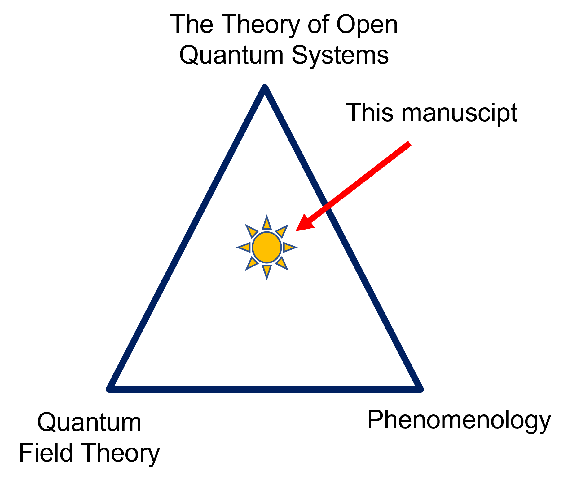
The challenges posed by the rapidly developing quantum technologies appear to exceed the applicability of theoretical methods that were successful in the past. In this way, the (purely) phenomenological description of interacting quantum systems seems too heuristic and insufficient to capture exclusively quantum phenomena of contemporary central interest. On the other hand, the great machinery of quantum field theory (QFT) fails to describe situations in which the system’s time evolution is a relevant figure of merit. For example, the description of quantum gates, elementary units of a quantum computer, in terms of IN (t=−∞t=-\infty) and OUT (t=+∞t=+\infty) states that are inherent for QFT treatment would be highly unsatisfactory as for the long times (t=+∞t=+\infty) the state of the system thermalizes. It is, therefore, crucial to develop a possibly accurate scheme in the language of the theory of open quantum systems. In this manuscript, we propose an approach to the reduced dynamics of open quantum systems that facilities the qualities of both phenomenological and field-theoretic description (see Figure 1). Namely, the dynamics is determined with just a few experimentally determined parameters and encompasses ideas from the QFT, such as renormalization and the dressing of systems.
Refer to caption
Figure 1: Picture illustrating the approach we assimilate in this manuscript.

The requirement for the weak interaction usually referred to as the Born approximation, is the heart of the dynamical equations of the theory of open quantum systems Breuer and Petruccione 2006. In a nutshell, the Born approximation consists of two steps: (i) the perturbative expansion of dynamics is truncated to the second-order with respect to coupling constant, (ii) the initial state of the total system is of the product form between the open system and the reservoir (cf. Alipour et al. 2020; Merkli 2021; Trushechkin 2021a). In particular, the famous Davies-GKSL11 1 Davies-Gorini–Kossakowski–Sudarshan–Lindblad. Markovian master equation is exceedingly successful in describing the evolution of open quantum systems in the weak coupling regime Davies 1974; Gorini et al. 1976; Lindblad 1976. Still, due to explicit separation of time scales concerning the internal evolution of the system and the reservoir relaxation rates, the Davis-GKSL equation in its different versions22 2 Here, we mean the ”global” and the ”local” approaches Cattaneo and Manzano 2021 can not simultaneously describe all time regimes of the evolution of the quantum system33 3 The initial (super-short) times t<1ωct<\frac{1}{\omega_{c}} are also (currently) out of reach for all (universal) dynamical equations that attempt to describe the dynamics using just a few phenomenological parameters. This limitation is because the initial dynamics depends on the cut-off frequency that is usually not well characterized and depends on the specific setup. On the other hand, we have to assume (at least) the pure existence of some cut-off frequency ωc\omega_{c} for the system Hamiltonians to be well defined.. On the other hand, the equally acclaimed Bloch-Redfield (master) equation does not distinguish any particular time scale and paves the way for the correct description in the whole time regime Bloch 1957; Redfield 1957. Unfortunately, the Bloch-Redfield equation violates positivity of the density operator as it is not of the Gorini–Kossakowski–Sudarshan–Lindblad (GKSL) form. The drawback of the dynamics not being CPTP is of fundamental importance, and for this reason, it has been addressed in literature many times. As a result, a plethora of different dynamical equations for the time evolution of the reduced density matrix of an open system has been constructed Schaller and Brandes 2008; Majenz et al. 2013; Davidović 2020; Trushechkin 2021b.

In general, all the standard approaches mentioned above contain the so-called Lamb-Stark shift term Breuer and Petruccione 2006. The presence of the aforementioned term in the dynamical equation leads to a (alleged) shift in the energy levels of the open system cause by the interaction with the environment. However, the dissipation still proceeds with respect to energy levels that are not shifted (renormalized). This leads to a thermodynamical inconsistency of the described approaches. On the one hand, the energy levels of the open system are renormalized via the Lamb-Stark shift term. On the other hand, the evolution leads to the stationary state with populations identical to Gibbs state with respect to a Hamiltonian in which energy levels are not shifted. Indeed, the Davies-GKSL equation predicts the stationary state to be a Gibbs state with respect to the not renormalized (bare) Hamiltonian, whereas the Bloch-Redfield equation predicts the same populations as the Davies-GKSL equation but exhibits steady-state coherence (see Ref. Łobejko et al. 2022 for detailed discussion). As the drawback of this inconsistency, the standard approaches always fail to correctly describe the stationary state and dissipation rates simultaneously. As we will show, this issue can be overcome with a proposed here renormalization procedure.

The first equation that yields CPTP dynamics and is relevant for all time scales (except initial times) was derived in Ref. Alicki 1989, and has been recently independently discovered by A. Rivas Rivas 2017, where the name refined weak coupling limit is used. This equation, for which we adapt the name the cumulant equation is one of the central objects in our considerations (see also reference Winczewski et al. 2021). The first derivation in Ref. Alicki 1989 is based on a deeper insight into the meaning of the Born approximation that employs the idea of quantum noise. Namely, in its first part, i.e. (i), the Born approximation refers to the description of the interaction between the open system and the reservoir in the spirit of the quantum analogs of the central limit theorem (CLT) Goderis et al. 1989; Goderis et al. 1990; Accardi et al. 1990; Accardi et al. 2002. In this manner, the interaction of the open system with the bath is expressed as a sum of numerous (ideally infinite) weak and independent perturbations. In principle, this form of interaction accounts for the open system to experience a (quantum) Gaussian noise due to the reservoir. On the other hand, this kind of characterization of the interaction has to be confronted with the Hamiltonian dynamics of the total system. Therefore, it is essential to decompose the quantum noise into two parts. The first component (drift) corresponds to the coherent evolution of the system. It contains Hamiltonian-like terms associated with the (bare) free Hamiltonian of the open system combined with possible (renormalization) corrections. The second part accounts for pure dissipation. At this place, the idea of renormalization enters the derivation of the cumulant equation. Namely, it is postulated that in the interaction picture with respect to the physical, renormalized Hamiltonian of the system, the dynamics should be purely dissipative, i.e., it should not contain any Hamiltonian-like terms.

In the interaction picture with respect to the physical (renormalized) Hamiltonian H𝒮H_{\mathcal{S}}, the reduced dynamics of the system 𝒮\mathcal{S} should be purely dissipative, i.e., it should not include any Hamiltonian-like terms.

In this manuscript, we refer to the above postulate as to the self-consistency condition. Indeed, the Hamiltonian-like terms (Lamb-Stark shift term) can be compensated with the aforementioned corrections to the bare Hamiltonian of the open system. As we discuss in this manuscript, the presence of the corrections is indispensably connected to the assumption of the initial state to be in the product form, i.e., the second part, (ii) of the Born approximation. However, the renormalization procedure that removes all Hamiltonian-like terms yields different dynamical equations than the standard derivation of Davies-GKSL Breuer and Petruccione 2006 or Bloch-Redfield equation, in which the Lamb-Stark shift term (Hamiltonian-like) is explicitly present44 4 Still, negligence of this term is a common practice.. As we show, the renormalized equations do not exhibit the aforementioned conflict in simultaneous prediction of the populations of the stationary state and the dissipation rates. Additionally, we take a chance to exhaustively explain the first derivation of the cumulant equation. Still, we do not hesitate to provide some minor generalizations and novel contributions.

In order to prove the relevance of the self-consistency condition, we firstly formulate an intuition about the return to the equilibrium in the open quantum system setting. The intuition prompts us that a joint quantum system consisting of the small system 𝒮\mathcal{S}, and a large reservoir ℛ\mathcal{R} in the thermal state (heat bath) should return to the equilibrium state whenever an interaction between the units is present. Moreover, because of the discrepancy in “sizes” of systems 𝒮\mathcal{S} and ℛ\mathcal{R}, and the requirement for weak interaction, the equilibrium state should be the global thermal state with the same temperature as the initial temperature of the reservoir ℛ\mathcal{R}. In fact, this intuition has its confirmation in mathematically rigorous results of the quantum theory of infinite systems Araki and Woods 1963; Araki 1973; Bratteli and Robinson 1987; Bratteli and Robinson 1997; Dereziński 2007. Therefore, the intuition we present allows us to ask an important question about the reduced state of the system 𝒮\mathcal{S} after the equilibrium is reached Hilt et al. 2011; Trushechkin et al. 2021.

If the reduced state of systems 𝒮\mathcal{S} is truly a Gibbs (thermal) state with inverse temperature β\beta then with respect to which Hamiltonian and what is its relation to the bare one?

The Hamiltonian in the above question is the so-called mean-force (Gibbs state) Hamiltonian Hilt et al. 2011; Trushechkin et al. 2021; Łobejko et al. 2022; Timofeev and Trushechkin 2022. Informally speaking, the mean-force Hamiltonian describes the ”effective” force exerted on the open system by the reservoir. In this manner, the relevance of the renormalization procedure for the dynamical equations is guaranteed via confronting it with the “static” results from the quantum theory of infinite systems Araki and Woods 1963; Araki 1973; Bratteli and Robinson 1987; Bratteli and Robinson 1997; Dereziński 2007. Moreover, the mean-force Hamiltonian approach provides a platform at which the interpretation of the Lamb-Stark shift term can be questioned.

The manuscript is organized as follows. In Section II we formulate the intuition about the relaxation to equilibrium for the total system. We expect that if the initial state of the reservoir is the thermal (KMS) state with the inverse temperature β\beta, then the total system will equilibrate to the global thermal (KMS) state with the same inverse temperature. In Section III we describe the specific system under the study in terms of Hamiltonians and initial states. Section IV is devoted to the analysis of the standard derivation of the Davies-GKSL equation Breuer and Petruccione 2006. In particular, we show how the first-order renormalization is built-in in the standard derivation of the Davies-GKSL equation. Furthermore, subsection IV.2 takes a deeper insight into problems concerning Lamb-Stark shift term from the phenomenological perspective. We discuss the problems concerning the presence of Lamb-Stark shift term and the condition for its negligence. The problem of inconsistency with thermodynamics in the standard approaches is remarked. In Section V we calculate the partial trace with respect to the reservoir of the total system 𝒮+ℛ\mathcal{S}+\mathcal{R} thermal (KMS) state, and in this way we rederive the so-called mean-force Hamiltonian Łobejko et al. 2022; Timofeev and Trushechkin 2022. This important technical result is obtained using Explicit description of the Zassenhaus formula obtained by T. Kimura Kimura 2017. The partial trace provides a “static” form of renormalization and the answer to the question stated before in Section II. In the next Section VI we sketch the derivation of the cumulant equation equation (the complete derivation is present in Section D of the Appendix). We discuss the relation between the cumulant equation and the Bloch-Redfield master equation. In particular, we transform the cumulant equation into a differential equation and show that the Bloch-Redfield equation emerges as its approximation. Furthermore, we calculate the long time-limit for the cumulant equation (cf. Rivas 2017), and discuss its stationary state Winczewski 2022. We show how the renormalization procedure motivated by the previously postulated self-consistency condition yield equations that reproduce the correct stationary state populations, i.e., populations of the Gibbs state with respect to the renormalized (physical) Hamiltonian. Section VII is devoted to the discussion about the physical meaning of the renormalization procedure, interpretation of the renormalized Hamiltonian, and the counterterms (Lamb-Stark shift term). Moreover, we provide a simplified scheme for the renormalization that can be applied to Davies-GKSL or Bloch-Redfield equations. The last Section VIII is left for the concluding remarks.

II Intuition

Our starting point is the intuition wandering around the zeroth law of thermodynamics. Still, the intuitive considerations present in this Section have their mathematically rigorous justification in the theory of infinite systems Araki and Woods 1963; Araki 1973; Bratteli and Robinson 1987; Bratteli and Robinson 1997; Dereziński 2007. Consider small quantum system 𝒮\mathcal{S}, and thermal reservoir (heat bath) ℛ\mathcal{R} at the inverse temperature β\beta. The heat bath is a much larger system than 𝒮\mathcal{S} as it possesses an infinite number of degrees of freedom contrary to small system 𝒮\mathcal{S}. The total, closed system 𝒮+ℛ\mathcal{S}+\mathcal{R} is prepared initially (at t=0t=0) in a product state ρ𝒮⊗ρℛ,β\rho_{\mathcal{S}}\otimes\rho_{\mathcal{R},\beta}. Where ρℛ,β\rho_{\mathcal{R},\beta} is a thermal (KMS) state of the reservoir, and ρ𝒮\rho_{\mathcal{S}} is unspecified, i.e., any possible state of 𝒮\mathcal{S}.

Refer to caption
Figure 2: Pictographic description on the initial state of the system. In the Born approximation the inital state is of the product form.

Suppose now that at time t=0t=0 the system 𝒮\mathcal{S} and the heat bath ℛ\mathcal{R} start to interact (see Figure 2). We assume here that the coupling is reasonably weak. Then, after a judiciously long time, a new equilibrium55 5 Precisely speaking, the state of the total system asymptotically approaches the equilibrium in the sense of locally measurable quantities. state is established, the form of which is dependent on the interaction. However, because of its size, the reservoir is scarcely affected by the interaction. Therefore, the new equilibrium state is perfectly approximated with KMS (thermal) state ρ𝒮+ℛ,β\rho_{\mathcal{S}+\mathcal{R},\beta}, with the same inverse temperature β\beta (see Figure 3). This approximation is the better, the larger is the heat bath, and the smaller is the system 𝒮\mathcal{S}. Alternatively, in this situation, one can think of system 𝒮\mathcal{S} as a perfect thermometer and ℛ\mathcal{R} as an examined object.

Refer to caption
Figure 3: Pictographic description on the initial state of the stationary state of the system established after long time since the interaction started.

One can ask now “what is the reduced state of the system 𝒮\mathcal{S}?”. The most obvious, and apparently almost correct, answer to this question is “thermal state with inverse temperature β\beta, i.e., ρ𝒮,β\rho_{\mathcal{S},\beta}”, however, this is not enough. Because the system SS is small, the interaction with a much larger system ℛ\mathcal{R} can alter its properties, e.g., energy levels. In this way, a more elaborate question arises on if the reduced state of systems 𝒮\mathcal{S} is truly a Gibbs (thermal) state with inverse temperature β\beta then with respect to which Hamiltonian and what is its relation to the bare one?. Finding the adequate Hamiltonian is, therefore, a matter of proper renormalization procedure. This task is a goal of the forthcoming Sections.

III The setup

In order to show and justify the idea of the renormalization procedure proposed by us, we consider the most basic, newbie training, yet nontrivial setup. In this way, we consider small, open quantum system 𝒮\mathcal{S} interacting with large quantum reservoir ℛ\mathcal{R} in a KMS state that we call the heat bath interchangeably. At this place, we would like to specify that by “small,” we mean a system with a discrete spectrum, e.g., a qubit, an atom or a molecule, and by “large,” we mean a reservoir with an infinite number of degrees of freedom that can be modeled by a large, i.e., numerous (ideally infinite), collection of non-interacting quantum harmonic oscillators (modes), e.g. electromagnetic, phonon or fermionic field.

We denote the states of any system 𝒜∈{𝒮,ℛ,𝒮+ℛ}\mathcal{A}\in\left\{\mathcal{S},\mathcal{R},\mathcal{S}+\mathcal{R}\right\}, with ρ𝒜∈ℬ⁡(ℋ𝒜)\rho_{\mathcal{A}}\in\mathcal{B}(\mathcal{H}_{\mathcal{A}}). Additionally, subscript β\beta in ρ𝒜,β\rho_{\mathcal{A},\beta}, referring to inverse temperature β\beta, stands for a system 𝒜\mathcal{A} being in the KMS (thermal) state defined with:

ρ𝒜,β:=Z𝒜−1​e−β​H𝒜,\displaystyle\rho_{\mathcal{A},\beta}:=Z_{\mathcal{A}}^{-1}e^{-\beta H_{\mathcal{A}}}, (1)
Z𝒜:=tr⁡[e−β​H𝒜],\displaystyle Z_{\mathcal{A}}:=\tr\left[e^{-\beta H_{\mathcal{A}}}\right], (2)

where Z𝒜−1Z_{\mathcal{A}}^{-1} is called the partition function.

Let, H𝒮(0)H_{\mathcal{S}}^{(0)} be the free (also called bare) Hamiltonian of the system 𝒮\mathcal{S}, and HℛH_{\mathcal{R}} be the Hamiltonian of the reservoir ℛ\mathcal{R}. Further, we chose the interaction Hamiltonian Hℐ(0)H^{(0)}_{\mathcal{I}} to have the following standard form:

Hℐ(0)=∑iSi⊗Ri(0),\displaystyle H^{(0)}_{\mathcal{I}}=\sum_{i}S_{i}\otimes R^{(0)}_{i}, (3)

with SiS_{i}, and Ri(0)R^{(0)}_{i} being self-adjoint operators. For simplicity we assume that SiS_{i}, and Ri(0)R^{(0)}_{i} are time independent (this assumption will be relaxed later in Section VI). Moreover we assume that the diagonal elements of interaction operators SiS_{i} are zero (See Remark 2). We also assume that the interaction does not allow for any dark (meta-stable) states that are decoupled, so that unique equilibrium state can be reached. In fact, this is the most physically relevant case as the higher-order contributions to the interaction finally reproduce the ergodicity. Additionally, we make a technical assumption on the spectral density of the reservoir. Namely, we assume that the spectral density of the reservoir does not grow exponentially for large frequencies.

Finally, we can write down the Hamiltonian of the total, closed system 𝒮+ℛ\mathcal{S}+\mathcal{R}:

H𝒮+ℛ=H𝒮(0)+Hℛ+λ​Hℐ(0),\displaystyle H_{\mathcal{S}+\mathcal{R}}=H^{(0)}_{\mathcal{S}}+H_{\mathcal{R}}+\lambda H^{(0)}_{\mathcal{I}}, (4)

where λ=1\lambda=1 is an auxiliary object, that will prove its usefulness in enumerating powers of the coupling constant in perturbative expansions.

Remark 1.

Through the manuscript we do not follow (unless specified otherwise) the usual assumption of Ri(0)R^{(0)}_{i} being centered with respect to the state of the reservoir, i.e., ⟨Ri(0)⟩ρℛ,β=0\left<R^{(0)}_{i}\right>_{\rho_{\mathcal{R},\beta}}=066 6 We follow a notation in which ⟨A⟩ρ=tr⁡[A​ρ].\left<A\right>_{\rho}=\tr\left[A\rho\right].. As we will show centering of Ri(0)R^{(0)}_{i} operators is the first step of the renormalization.

Remark 2.

For the sake of simplicity, we assume that the diagonal elements of SiS_{i} vanish (in the measurable energy eigenbasis). This ensures us that close to equilibrium the “mean force” that the system 𝒮\mathcal{S} exerts on the reservoir ℛ\mathcal{R} vanishes. This is the mirrored situation to the “centering” of reservoir operators described in Remark 1. An opposite case in which diagonal elements of SiS_{i} do not vanish should be treated, for example, with the polaron transform.

IV Case study: Davies-GKSL equation

In this Section, we consider a situation in which one is interested in the time evolution of the open system 𝒮\mathcal{S} in the setup described in Section III. However, our focus is concentrated much more on the stationary state (if it exists) obtained at the end of the evolution, that is, when t→+∞t\to+\infty.

One of the possibilities is to make use of the Davies-GKSL equation (Markovian master equation in secular approximation) that is known to be extremely successful in describing the dynamics of open quantum systems in weak coupling regime Davies 1974; Gorini et al. 1976; Lindblad 1976. Due to the secular approximation performed in the microscopic derivation of the Davies-GKSL equation, the validity of its solution is limited to the time scales that are not too short. Nonetheless, the stationary state, obtained for very long times, should be devoid of this limitation and therefore correctly determined.

IV.1 The stationary state - the first step of renormalization

In the Davies-GKSL equation that is derived under Born approximation the initial state is assumed to be a product ρ𝒮⊗ρ𝒮,β\rho_{\mathcal{S}}\otimes\rho_{\mathcal{S},\beta}. Then, provided Hℐ(0)H^{(0)}_{\mathcal{I}} is such that quantum dynamical semigroup generated by Davies-GKSL equation is ergodic Spohn 1977; Fagnola and Rebolledo 2001, and operators Ri(0)R^{(0)}_{i} are centered, i.e., ⟨Ri(0)⟩ρℛ,β=0\left<R^{(0)}_{i}\right>_{\rho_{\mathcal{R},\beta}}=0, there exists the unique stationary state Breuer and Petruccione 2006. The latter condition, is however not satisfied a priory in our case (see Remark 1).

Still, one can recover the standard approach to the Davies-GKSL equation if prior to the derivation we reshuffle terms in equation (4) so that the total Hamiltonian H𝒮+ℛH_{\mathcal{S}+\mathcal{R}} stays unchanged:

H𝒮(0)⟶H𝒮(1)=H𝒮(0)+∑iSi​⟨Ri(0)⟩ρℛ,β,\displaystyle H^{(0)}_{\mathcal{S}}\longrightarrow H^{(1)}_{\mathcal{S}}=H_{\mathcal{S}}^{(0)}+\sum_{i}S_{i}\left<R^{(0)}_{i}\right>_{\rho_{\mathcal{R},\beta}}, (5)
Hℐ(0)⟶Hℐ(1)=Hℐ(0)−∑iSi​⟨Ri(0)⟩ρℛ,β.\displaystyle H^{(0)}_{\mathcal{I}}\longrightarrow H^{(1)}_{\mathcal{I}}=H_{\mathcal{I}}^{(0)}-\sum_{i}S_{i}\left<R^{(0)}_{i}\right>_{\rho_{\mathcal{R},\beta}}. (6)

In this way the above transformation defines the centered operators Ri(1)R^{(1)}_{i}, and centered interaction Hamiltonian

Ri(1)=Ri(0)−⟨Ri(0)⟩ρℛ,β,\displaystyle R^{(1)}_{i}=R^{(0)}_{i}-\left<R^{(0)}_{i}\right>_{\rho_{\mathcal{R},\beta}}, (7)
Hℐ(1)=∑iSi⊗Ri(1),\displaystyle H^{(1)}_{\mathcal{I}}=\sum_{i}S_{i}\otimes R^{(1)}_{i}, (8)

Additionally H𝒮(1)H^{(1)}_{\mathcal{S}} is now the new (first-order renormalized) Hamiltonian of the system 𝒮\mathcal{S}, that defines the stationary state

ρ𝒮,β(1)=Z𝒮(1)−1​e−β​H𝒮(1),Z𝒮(1)=tr⁡[e−β​H𝒮(1)],\displaystyle\rho^{(1)}_{\mathcal{S},\beta}={Z^{(1)}_{\mathcal{S}}}^{-1}e^{-\beta H^{(1)}_{\mathcal{S}}},\penalty\ \penalty\ Z^{(1)}_{\mathcal{S}}=\tr\left[e^{-\beta H^{(1)}_{\mathcal{S}}}\right], (9)

of the Davies-GKSL equation that following the standard miscroscopic derivation Breuer and Petruccione 2006 has the form (in Schrödinger picture):

dd​t​ρ𝒮​(t)=L​ρ𝒮​(t)\displaystyle\frac{d}{dt}{\rho}_{\mathcal{S}}(t)=L{\rho}_{\mathcal{S}}(t) (10)
=−i⁡[H𝒮(1)+λ2​HL​S,ρ𝒮​(t)]+λ2​𝒟​(ρ𝒮​(t)),\displaystyle=-i\left[H_{\mathcal{S}}^{(1)}+\lambda^{2}H_{LS},{\rho}_{\mathcal{S}}(t)\right]+\lambda^{2}\mathcal{D}({\rho}_{\mathcal{S}}(t)), (11)

where LL is the generator of the quantum dynamical semigroup of the Davies-GKSL equation and 𝒟​(ρ𝒮​(t))\mathcal{D}({\rho}_{\mathcal{S}}(t)) is a component of the Davies-GKSL equation so-called the dissipator defined with:

𝒟⁡(ρ𝒮​(t))=∑ω1∑i​jγi​j​(ω1)\displaystyle\mathcal{D}({\rho}_{\mathcal{S}}(t))=\sum_{\omega_{1}}\sum_{ij}\gamma_{ij}(\omega_{1})
×(Sj​(ω1)​ρ𝒮​(t)​Si†​(ω1)−12​{Si†​(ω1)​Sj​(ω1),ρ𝒮​(t)}).\displaystyle\times\left(S_{j}(\omega_{1}){\rho}_{\mathcal{S}}(t)S_{i}^{\dagger}(\omega_{1})-\frac{1}{2}\left\{S_{i}^{\dagger}(\omega_{1})S_{j}(\omega_{1}),{\rho}_{\mathcal{S}}(t)\right\}\right). (12)

In the above sum, {ω1}\{\omega_{1}\}’s are the Bohr frequencies of the system 𝒮\mathcal{S} calculated with respect to the Hamiltonian H𝒮(1)H^{(1)}_{\mathcal{S}}77 7 In the manuscript, we assimilate a notation in which Bohr frequencies of Hamiltonians H𝒮(k)H_{\mathcal{S}}^{(k)} are denoted ωk\omega_{k}, for k=0,1,2k=0,1,2.. Furthermore,

HL​S=∑ω1∑i​j𝒮i​j​(ω1)​Si†​(ω1)​Sj​(ω1),\displaystyle H_{LS}=\sum_{\omega_{1}}\sum_{ij}\mathcal{S}_{ij}(\omega_{1})S_{i}^{\dagger}(\omega_{1})S_{j}(\omega_{1}), (13)

is the Lamb-Stark shift Hamiltonian, and

γi​j​(ω)=Γi​j​(ω)+Γj​i∗​(ω),\displaystyle\gamma_{ij}(\omega)=\Gamma_{ij}(\omega)+\Gamma^{*}_{ji}(\omega), (14)

are the Markovian relaxation rates. The above objects can be calculated with

𝒮i​j​(ω)=Γi​j​(ω)−Γj​i∗​(ω)2​i,\displaystyle\mathcal{S}_{ij}(\omega)=\frac{\Gamma_{ij}(\omega)-\Gamma^{*}_{ji}(\omega)}{2i}, (15)
Γi​j​(ω)=∫0+∞d​s​ei​ω​s​⟨R~i(1)​(s)​Rj(1)⟩ρℛ,β,\displaystyle\Gamma_{ij}(\omega)=\int_{0}^{+\infty}ds\penalty\ e^{i\omega s}\left<\tilde{R}^{(1)}_{i}(s)R^{(1)}_{j}\right>_{\rho_{\mathcal{R},\beta}}, (16)
Si​(ω1)=∑ϵ1′−ϵ1=ω1Π⁡(ϵ1)​Si​Π​(ϵ1′),\displaystyle S_{i}(\omega_{1})=\sum_{\epsilon^{\prime}_{1}-\epsilon_{1}=\omega_{1}}\Pi(\epsilon_{1})S_{i}\Pi(\epsilon^{\prime}_{1}), (17)

where Π⁡(ϵ1)\Pi(\epsilon_{1}) are projections into eigenspaces of H𝒮(1)H^{(1)}_{\mathcal{S}} associated with eigenvalues {ϵ1}\{\epsilon_{1}\} (see Section A for more details).

The above result, despite its triviality, can be seen as the first step of renormalization. Indeed, the relaxed and recovered later on assumption (see Remark 1) is very often satisfied from the very beginning. On the other hand, the interaction changes the properties of the system 𝒮\mathcal{S}, in such a way that the new, first-order renormalized Hamiltonian H𝒮(1)H^{(1)}_{\mathcal{S}} must be considered in order to describe its dynamics and stationary state of Davies-GKSL equation correctly.

Suppose now that the Davies-GKSL equation correctly predicts the reduced state of the system 𝒮\mathcal{S} after the equilibrium is reached. Then the above considerations, on the contrary to their triviality, show that the question stated in Section II, about Hamiltonian with respect to which the reduced state of the system 𝒮\mathcal{S} is a Gibbs (thermal) state is nontrivial itself. This nontriviality is because one can wrongly associate the reduced state of the system 𝒮\mathcal{S} with H𝒮(0)H^{(0)}_{\mathcal{S}} instead of H𝒮(1)H^{(1)}_{\mathcal{S}}, if the analysis of the form of interaction is skipped. This is because the interaction Hamiltonian Hℐ(1)H^{(1)}_{\mathcal{I}} determines the reduced state of the system 𝒮\mathcal{S} after the equilibrium is reached. In the next Section, we discuss if another steps of the renormalization are required for the dynamical equation to satisfy thermodynamical consistency.

IV.2 Lamb-Stark shift term - the next renormalization step

Let us analyze in this place one more element of the Davies-GKSL equation. The term including HL​SH_{LS} is usually referred to as a term including Lamb (vacuum) and Stark (reservoir’s state-dependent) shifts that lead to the renormalization of eigenstates of H𝒮(1)H^{(1)}_{\mathcal{S}}. For the sake of the clarity of the presentation, let us assume in this Section that the quantities in equations (14)-(15) can be written in the following form88 8 The state of the reservoir is still the KMS state, that is in this case a quasi-free gauge-invariant state completely characterized by the occupation numbers.:

γi​j​(ω)=Ji​j​(ω)​(Nβ​(ω)+1),\displaystyle\gamma_{ij}(\omega)=J_{ij}(\omega)\left(N_{\beta}(\omega)+1\right), (18)
𝒮i​j(ω)=−∫0ωcdΩJi​j(Ω)(Nβ​(ω)+1ω−Ω+Nβ​(ω)ω+Ω),\displaystyle\mathcal{S}_{ij}(\omega)=\mathchoice{{\vbox{\hbox{$\textstyle-$}}\kern-4.86108pt}}{{\vbox{\hbox{$\scriptstyle-$}}\kern-3.43057pt}}{{\vbox{\hbox{$\scriptscriptstyle-$}}\kern-2.908pt}}{{\vbox{\hbox{$\scriptscriptstyle-$}}\kern-2.76045pt}}\!\int_{0}^{\omega_{c}}d\Omega\penalty\ J_{ij}(\Omega)\left(\frac{N_{\beta}(\omega)+1}{\omega-\Omega}+\frac{N_{\beta}(\omega)}{\omega+\Omega}\right), (19)

where Ji​jJ_{ij} is the so-called spectral density function, NβN_{\beta} is the Bose–Einstein distribution distribution, ωc\omega_{c} is the cut-off frequency and −⁣∫\mathchoice{{\vbox{\hbox{$\textstyle-$}}\kern-4.86108pt}}{{\vbox{\hbox{$\scriptstyle-$}}\kern-3.43057pt}}{{\vbox{\hbox{$\scriptscriptstyle-$}}\kern-2.908pt}}{{\vbox{\hbox{$\scriptscriptstyle-$}}\kern-2.76045pt}}\!\int denotes the Cauchy’s principal value of the integral. Nonetheless, the above assumption is valid for the majority of the situations considered in the literature.

However, the presence of the Lamb-Stark shift term in equation (11) leads to the inconsistency because dissipation governs by other terms (the dissipator) in equation (13) is assumed to happen with respect to energy levels of the open system 𝒮\mathcal{S} that are not renormalized (not shifted). Moreover, only for the case of negligible small Lamb-Stark shift associated with HL​SH_{LS} the equation (11) is consistent with thermodynamics. Namely, for the thermal bath at the inverse temperature β\beta, due to KMS condition for the correlation functions ⟨Ri(1)​(s)​Rj(1)⟩ρℛ,β\left<{R}^{(1)}_{i}(s)R^{(1)}_{j}\right>_{\rho_{\mathcal{R},\beta}}, the additional relation holds:

γi​j​(−ω)=e−β​ω​γj​i​(ω).\displaystyle\gamma_{ij}(-\omega)=e^{-\beta\omega}\gamma_{ji}(\omega). (20)

Therefore, the dynamics in equation (11) drives the open quantum system 𝒮\mathcal{S} to the Gibbs state defined by the bare Hamiltonian H𝒮(1)H_{\mathcal{S}}^{(1)} and not, as expected on the thermodynamic ground, the (alleged99 9 As we show later, the interpretation of the Lamb-Stark shift term is (at least) questionable.) physical one containing the Lamb-Stark shift H𝒮(1)+HL​SH_{\mathcal{S}}^{(1)}+H_{LS}.

To discuss the problem of Lamb-Stark shift computation and its relevance for the real system, we consider a bath consisting of many harmonic oscillators such that

Hℐ(1)=λ​S⊗∑k(g¯​(k)​bk+g⁡(k)​bk†),\displaystyle H_{\mathcal{I}}^{(1)}=\lambda\penalty\ S\otimes\sum_{k}\left(\bar{g}(k)b_{k}+g(k)b^{\dagger}_{k}\right), (21)
Hℛ=∑kω⁡(k)​bk†​bk.\displaystyle\quad H_{\mathcal{R}}=\sum_{k}\omega(k)b^{\dagger}_{k}b_{k}. (22)

While for a finite number of bath’s oscillators, the total Hamiltonian H𝒮+ℛ=H𝒮+Hℛ+HℐH_{\mathcal{S}+\mathcal{R}}=H_{\mathcal{S}}+H_{\mathcal{R}}+H_{\mathcal{I}} is well-defined, the models with their infinite number, in particular, the infinite volume baths need special attention (cf. reference Rivas et al. 2010). Namely, it is well-known that in those physically important cases, the following additional conditions (written in the continuous modes notation)

∫|g⁡(k)|2​ω​(k)−2​𝑑k<∞\int|g(k)|^{2}\omega(k)^{-2}\,dk<\infty (23)

must be fulfilled to yield a self-adjoint and possess a ground state Hamiltonian H𝒮+ℛH_{\mathcal{S}+\mathcal{R}}. For realistic models with physically justified dispersion ω⁡(k)\omega(k), this means a suitable behavior of the coupling magnitude |g⁡(k)||g(k)| at low-frequency modes (avoiding ‘‘infrared catastrophe”)1010 10 For example, a very popular Ohmic coupling is excluded. and its strong enough suppression for high frequencies usually characterized by the “ultraviolet cut-off” frequency ωc\omega_{c}.

Importantly, as long as ω<ωc\omega<\omega_{c}, the values of the relaxation rates γi​j​(ω)\gamma_{ij}(\omega) do not depend on the cut-off, while the Lamb shift is strongly dependent on it and typically diverges with ωc→∞\omega_{c}\to\infty (see equations (18)- (19)).

In principle, the Lamb-Stark shift effect could be ignored if (i) it is proportional to λn\lambda^{n}, with n>2n>2 (Born approximation) or (ii) it is just small (cf. reference Rivas 2017). Nonetheless, (i) does not hold because the term with HL​SH_{LS} is proportional to λ2\lambda^{2} exactly the same as the dissipator, and (ii) does not hold in general (on the contrary to fully relativistic field-theoretic calculations). Moreover, if the spectral density of the reservoir ℛ\mathcal{R} does not contain a natural cut-off ωc\omega_{c}, just as in an extremely important case of electromagnetic field, then HL​SH_{LS} contains integrals with irremovable divergences. This divergence makes the whole Davies-GKSL is ill-defined1111 11 If any auxiliary cut-off that regularizes the dynamical equation is introduced, then the resulting dynamics shall not depend on the value of its parameters.. In this case, one of the solutions encountered in the literature is not to include the Lamb-Stark shift term, which is (as we show) equivalent to stating that H𝒮(1)H^{(1)}_{\mathcal{S}} is already renormalized, physically relevant, and measurable Hamiltonian of the system 𝒮\mathcal{S}. In this way, self-consistency is recovered since the correct (renormalized) Bohr frequencies enter the dissipator. On the other, this drawback can be fixed using the derivation in the interaction picture with respect to the already renormalized physical Hamiltonian. The justification for the equivalence between the two renormalization methods will be presented in the rest of this manuscript.

To illustrate the physical meaning of ωc\omega_{c}, we consider two examples of qubits (fermionic oscillators) interacting with bosonic fields and present the relevant frequency scales.

  1. 1.

    Atom interacting with electromagnetic field, ω∼1015​H​z\omega\sim 10^{15}Hz, |γi​i​(ω)|∼109​s−1\absolutevalue{\gamma_{ii}(\omega)}\sim 10^{9}s^{-1} ; ωc\omega_{c} is not precisely defined, sometimes identified as ωc∼c/a0≃1019​H​z\omega_{c}\sim c/a_{0}\simeq 10^{19}Hz, (a0a_{0} - the Bohr radius, cc - the speed of light in vacuum).

  2. 2.

    Superconducting qubit interacting with phonons, ω∼5⋅109​H​z\omega\sim 5\cdot 10^{9}Hz, |γi​i​(ω)|∼104​s−1\absolutevalue{\gamma_{ii}(\omega)}\sim 10^{4}s^{-1} ; ωc\omega_{c} is identified with the Debye frequency ωD∼1013​H​z\omega_{D}\sim 10^{13}Hz.

In both cases, the separation of relevant frequency (or time) scales, |γi​j​(ω)|<<ω<<ωc\absolutevalue{\gamma_{ij}(\omega)}<<\omega<<\omega_{c}, is by the four to six orders of magnitude what implies the validity of the Markovian approximation in the weak coupling limit approach (cf. reference Rivas 2017). The cut-off frequency inserted into the definition of interaction Hamiltonian makes the corresponding effective theory mathematically consistent and applicable to physical phenomena characterized by time scales much longer than 1/ωc1/\omega_{c}. However, in both representative cases above, the Lamb-Stark shift computed using the renormalized equation is physically meaningless. In the case of an atom interacting with the electromagnetic field, we must refer to the higher-level theory - the quantum electrodynamics, while for the superconducting qubit, we must use phenomenological values because the linear (in bk,bk†b_{k},b^{\dagger}_{k}) interaction Hamiltonian is only a low energy approximation, insufficient to account for corrections to bare Hamiltonian generated by higher-order terms.

Summarizing, the consistent approach to the quantum master equations obtained in the weak coupling limit approach (like the Davies-GKSL equation (11)) involves two steps: 1) determination of the physical Hamiltonian H𝒮H_{\mathcal{S}} of the open system 𝒮\mathcal{S} using either its measured Bohr frequencies, or referring to the renormalization procedure within a higher level, more fundamental theory; 2) determination of the relaxation parameters which can be measured, or computed using the cut-off independent formulas, applied to the low energy effective Hamiltonian H𝒮H_{\mathcal{S}}.

Remark 3.

The renormalization procedure for the Lamb -Stark corrections is important not only for a single open system interacting with a reservoir, as it also describes the effects of interaction between many subsystems mediated by a shared reservoir. For example, for an ensemble of two-level “atoms” localized at different sites and interacting with an electromagnetic field, the total Lamb-Stark correction contains not only (cut-off dependent) individual energy shifts but also two-body (cut-off independent) interactions interpreted as Van der Waals dipole-dipole coupling Gross and Haroche 1982; Alicki and Lendi 1987.

V Partial trace of the total 𝒮+ℛ\mathcal{S}+\mathcal{R} system KMS state

We note that the results presented in this section were initially obtained in reference Łobejko et al. 2022 (see also Ref. Timofeev and Trushechkin 2022). Still, for the sake of completeness of the paper and due to an alternative derivation technique we do not hesitate to display them. Here, we would like to get back to the idea presented in Section II. In this place, without any reference to dynamical equations governing the time evolution of the reduced state of the system 𝒮\mathcal{S} we shall find the reduced state of the system 𝒮\mathcal{S} provided the state of the total system 𝒮+ℛ\mathcal{S}+\mathcal{R} is a KMS state

ρ𝒮=trℛ⁡[ρ𝒮+ℛ,β]=trℛ⁡[e−β⁡(H𝒮+Hℛ+λ​Hℐ)Z𝒮+ℛ,β].\displaystyle\rho_{\mathcal{S}}=\tr_{\mathcal{R}}\left[\rho_{\mathcal{S}+\mathcal{R},\beta}\right]=\tr_{\mathcal{R}}\left[\frac{e^{-\beta\left(H_{\mathcal{S}}+H_{\mathcal{R}}+\lambda H_{\mathcal{I}}\right)}}{Z_{\mathcal{S}+\mathcal{R},\beta}}\right]. (24)

In this way, we formulate the “static” argument for the justification of the self-consistency condition that we postulate.

In order to achieve our goal, without the loss of generality, we assume that the reduced state of the system 𝒮\mathcal{S} is of the following form:

ρ𝒮,β(m​f)=e−β​H𝒮(m​f)Z𝒮,β,\displaystyle\rho_{\mathcal{S},\beta}^{(mf)}=\frac{e^{-\beta H^{(mf)}_{\mathcal{S}}}}{Z_{\mathcal{S,\beta}}}, (25)
H𝒮(m​f)=H𝒮(0)+∑k=1∞λk​Hm​f,𝒞(k).\displaystyle H^{(mf)}_{\mathcal{S}}=H_{\mathcal{S}}^{(0)}+\sum_{k=1}^{\infty}\lambda^{k}H_{mf,\mathcal{C}}^{(k)}. (26)

Indeed, the reduced state of the system 𝒮\mathcal{S} should only depend on the bare Hamiltonian H𝒮(0)H_{\mathcal{S}}^{(0)}, the interaction Hamiltonian Hℐ(0)H_{\mathcal{I}}^{(0)}, and the state of the reservoir ρℛ,β\rho_{\mathcal{R},\beta}. With the form given in equation (25) in the case of no interaction the Gibbs (thermal) state of the system 𝒮\mathcal{S} with respect to H𝒮(0)H_{\mathcal{S}}^{(0)} is correctly recovered.

In the above formula operators, Hm​f,𝒞(k)H_{mf,\mathcal{C}}^{(k)} are different orders corrections to the bare Hamiltonian of the system 𝒮\mathcal{S} that are about to be determined. In order to achieve this task1212 12 Cf. for parallel works Łobejko et al. 2022; Timofeev and Trushechkin 2022 we different techniques are applied., we make use of an explicit description of the Zassenhaus formula proposed by T. Kimura in reference Kimura 2017 (cf. reference Purkayastha et al. 2020; Mori and Miyashita 2008; Hilt et al. 2011; Trushechkin et al. 2021). Despite the fact that the technique employed by us allows calculating the corrections of any order, we limit ourselves to the first two corrections Hm​f,𝒞(1)H_{mf,\mathcal{C}}^{(1)}, Hm​f,𝒞(2)H_{mf,\mathcal{C}}^{(2)}. This simplification is because, due to the Born approximation, the dynamical equations considered in this manuscript are limited to the second-order in λ\lambda order as well. Therefore, a renormalization of H𝒮(0)H_{\mathcal{S}}^{(0)} up to the second-order is sufficient for our purposes.

We find the first two corrections to the bare Hamiltonian H𝒮(0)H_{\mathcal{S}}^{(0)} of the system 𝒮\mathcal{S} to be expressed in terms of interaction operators (see equations (15-17))

Hm​f,𝒞(1)=∑iSi​⟨Ri(0)⟩ρℛ,β,\displaystyle H_{mf,\mathcal{C}}^{(1)}=\sum_{i}S_{i}\left<R_{i}^{(0)}\right>_{\rho_{\mathcal{R},\beta}}, (27)
Hm​f,𝒞(2)=∑ω1,ω1′∑i​jΥi​j(2)​(ω1,ω1′)​Si†​(ω1)​Sj​(ω1′),\displaystyle H_{mf,\mathcal{C}}^{(2)}=\sum_{{\omega_{1}},{\omega_{1}}^{\prime}}\sum_{ij}\Upsilon^{(2)}_{ij}({\omega_{1}},{\omega_{1}}^{\prime})S_{i}^{\dagger}({\omega_{1}})S_{j}({\omega_{1}}^{\prime}), (28)
Υi​j(2)​(ω1,ω1′)=1eβ⁡(ω1′−ω1)−1​(eβ⁡(ω1′−ω1)​𝒮i​j​(ω1)−𝒮i​j​(ω1′)CLOSE\displaystyle\Upsilon^{(2)}_{ij}({\omega_{1}},{\omega_{1}}^{\prime})=\frac{1}{e^{\beta({\omega_{1}}^{\prime}-{\omega_{1}})}-1}\left(e^{\beta(\omega_{1}^{\prime}-\omega_{1})}\mathcal{S}_{ij}(\omega_{1})-\mathcal{S}_{ij}(\omega_{1}^{\prime})\right.
OPEN−eβ​ω1′​(𝒮j​i​(−ω1′)−𝒮j​i​(−ω1))),\displaystyle\left.-e^{\beta\omega_{1}^{\prime}}\left(\mathcal{S}_{ji}(-\omega_{1}^{\prime})-\mathcal{S}_{ji}(-\omega_{1})\right)\right), (29)

where the terms for which ω′=ω\omega^{\prime}=\omega are determined via a limiting procedure ω′→ω\omega^{\prime}\to\omega

Υi​j(2)​(ω1,ω1)=𝒮i​j​(ω1)\displaystyle\Upsilon^{(2)}_{ij}({\omega_{1}},{\omega_{1}})=\mathcal{S}_{ij}(\omega_{1})
−1β​(∂∂ω1​𝒮i​j​(ω1)+eβ​ω1​∂∂ω1​𝒮j​i​(−ω1)).\displaystyle-\frac{1}{\beta}\left(\frac{\partial}{\partial\omega_{1}}\mathcal{S}_{ij}(\omega_{1})+e^{\beta\omega_{1}}\frac{\partial}{\partial\omega_{1}}\mathcal{S}_{ji}(-\omega_{1})\right). (30)

It is therefore evident that the mean-force Hamiltonian correction leads to a different prediction for the renormalization of the energy levels than the Lamb-Shift terms present in the Davies-GKSL (see equation (11)) or the Bloch-Redfield equation Cattaneo et al. 2019.

The formulas (27) and (28) above define the second-order approximation for the Hamiltonian H𝒮(m​f)H^{(mf)}_{\mathcal{S}}, and the state after the partial trace (we skip λ=1\lambda=1 lastly):

H𝒮(m​f)≈H𝒮(m​f,2)=H𝒮(0)+Hm​f,𝒞(1)+Hm​f,𝒞(2),\displaystyle H_{\mathcal{S}}^{(mf)}\approx H_{\mathcal{S}}^{(mf,2)}=H_{\mathcal{S}}^{(0)}+H_{mf,\mathcal{C}}^{(1)}+H_{mf,\mathcal{C}}^{(2)}, (31)
ρ𝒮,β(m​f)≈ρ𝒮,β(m​f,2)=e−β​H𝒮(m​f,2)Z𝒮,β(m​f,2).\displaystyle\rho^{(mf)}_{\mathcal{S},\beta}\approx\rho_{\mathcal{S},\beta}^{(mf,2)}=\frac{e^{-\beta H_{\mathcal{S}}^{(mf,2)}}}{Z_{\mathcal{S},\beta}^{(mf,2)}}. (32)

The details of the calculations of the partial trace are present in Section C of the Appendix.

In the first correction Hm​f,𝒞(1)H_{mf,\mathcal{C}}^{(1)}, in the equation (27), we recognize the correction that was also incorporated in the standard microscopic derivation of the Davies-GKSL equation (see equations (5)–(6) in Section IV), namely the centering of the interaction correction. This correspondence certifies that the requirement for the operators Ri(1)R_{i}^{(1)} to be centered with respect to the state of the heat bath is essential for reproducing the renormalized, physical Hamiltonian H𝒮H_{\mathcal{S}}.

On the other hand, the presence of the second-order correction Hm​f,𝒞(2)≠0H_{mf,\mathcal{C}}^{(2)}\neq 0 that we obtained shows that incorporating only the first-order correction to the bare Hamiltonian H𝒮(0)H^{(0)}_{\mathcal{S}} is not enough for the stationary state of the Davies-GKSL in equation (9) to be consistent with the second-order Born approximation and thermodynamics. Additionally, we note that [H𝒮(1),Hm​f​𝒞(2)]≠0\left[H_{\mathcal{S}}^{(1)},H_{mf\mathcal{C}}^{(2)}\right]\neq 0, what means that the interaction indeed changes the properties of the system 𝒮\mathcal{S}. This change has a physical interpretation in terms of the dressing of the bare system 𝒮\mathcal{S} with the excitations of the reservoir ℛ\mathcal{R} that emerge as a result of the interaction.

The incompatibility between the Lamb-Stark shift Hamiltonian HL​SH_{LS} and the second-order correction Hm​f,𝒞(2)H_{mf,\mathcal{C}}^{(2)} emphasizes the importance of the correct renormalization procedure for the treatment of open quantum systems. This is because the discrepancy mentioned above questions the interpretation of the Lamb-Stark shift term. Indeed, the comparison between HL​SH_{LS} and Hm​f,𝒞(2)H_{mf,\mathcal{C}}^{(2)} indicates that the Lamb-Stark shift term HL​SH_{LS} does not describe accurately the shift of energy levels caused by the interaction with the reservoir. As we show in the next Section VI the self-consistency condition fixes the renormalization procedure and removes the controversy described above.

Remark 4.

In fact, the Lamb-Stark shift term HL​SH_{LS} and the mean-force correction Hm​f,𝒞(2)H_{mf,\mathcal{C}}^{(2)} emerge from different perspectives, i.e, from the static and dynamical pictures Łobejko et al. 2022. As we suggest, this is the Lamb-Stark shift term HL​SH_{LS} that is misinterpreted and does not accurately describe any physical process (except for the coherent/drift part of quantum noise). However, an experiment would be necessary for the final verification of which correction accurately describes the shift of energy levels (see an experimental proposal in ref. Gramich et al. 2011).

VI The cumulant equation

In this Section we present the dynamical equation governing the time evolution of an open quantum system, in which the renormalization of the open system Hamiltonian is inalienable. This type of dynamical equations was firstly derived in reference Alicki 1989, and has been recently independently discovered by A. Rivas in reference Rivas 2017, where the name refined weak coupling limit was used (see also Majenz et al. 2013). Still, we use the nomenclature recently introduced in reference Winczewski et al. 2021. However, in the derivation in the reference Rivas 2017, due to different derivation techniques, the need for renormalization is not discussed. Therefore we base on the first derivation in the reference Alicki 1989.

VI.1 The derivation

The derivation of the cumulant equation in reference Alicki 1989 is based on different ideas than the derivation of the Davies-GKSL equation, but on the contrary to the latter, the cumulant equation is exact up to the Born approximation that is incorporated in both derivations. For the sake of generality, in the derivation, we relax the assumption on the reservoir state to be fixed to the KMS state. Instead, we assume that its state is stationary, i.e., [Hℛ,ρℛ]=0\left[H_{\mathcal{R}},\rho_{\mathcal{R}}\right]=0. Moreover, we assume that the total Hamiltonian of the open system 𝒮\mathcal{S}, and the reservoir ℛ\mathcal{R} before the renormalization is of the following, time-dependent form:

H𝒮+ℛ=H𝒮(0)​(t)+Hℛ+λ​Hℐ(0)​(t),\displaystyle H_{\mathcal{S}+\mathcal{R}}=H_{\mathcal{S}}^{(0)}(t)+H_{\mathcal{R}}+\lambda H_{\mathcal{I}}^{(0)}(t), (33)
Hℐ(0)​(t)=∑iSi⊗Ri(0)​(t).\displaystyle H_{\mathcal{I}}^{(0)}(t)=\sum_{i}S_{i}\otimes R^{(0)}_{i}(t). (34)

The relaxation of an assumption on the time-independence for the bare system and interaction Hamiltonians allows for understanding the behavior of the total system 𝒮+ℛ\mathcal{S}+\mathcal{R} in the spirit of the quantum field theory (QFT). This kind of treatment is the most adequate in realistic situations in which effects of state preparation and finite time of initiating the interaction have to be considered. The proposed relaxation helps us to bypass the aforementioned issues. Undoubtedly, to correctly understand the renormalization procedure, we have to consider the presence of the dressing processes that can be explained solely by field theoretical (QFT) considerations. At the same time, we assume that the total Hamiltonian of the system 𝒮+ℛ\mathcal{S}+\mathcal{R}, is approximately time-independent in a manner explained in Section D of the Appendix, where the details of the derivation are presented.

The renormalization procedure enters the derivation of the cumulant equation in a similar manner as it was in the case of the centering of interaction procedure in the derivation of Davies-GKSL equation (see Section IV.1). Namely, we postulate the existence of the following corrections to the bare Hamiltonian H𝒮(0)H_{\mathcal{S}}^{(0)} of the system 𝒮\mathcal{S}, and the interaction Hamiltonian Hℐ(0)H_{\mathcal{I}}^{(0)}, that give rise to the renormalized, physical Hamiltonian of the open system H𝒮H_{\mathcal{S}}, and the renormalized interaction Hamiltonian HℐH_{\mathcal{I}}. Indeed, we treat here Hamiltonians H𝒮(0)H_{\mathcal{S}}^{(0)}, and Hℐ(0)H_{\mathcal{I}}^{(0)} as auxiliary objects, whereas only the renormalized species, e.g., H𝒮H_{\mathcal{S}}, have physical relevance and can be empirically determined. This assignment reflects field-theoretical (QFT) that we (almost) never observe the bare particles. Instead, what we observe in the laboratory are the dressed particles evolution of which is governed by effective Hamiltonians.

H𝒮\displaystyle H_{\mathcal{S}} =H𝒮(0)​(t)+H𝒞​(t),\displaystyle=H_{\mathcal{S}}^{(0)}(t)+H_{\mathcal{C}}(t), (35)
Hℐ\displaystyle H_{\mathcal{I}} =Hℐ(0)​(t)−H𝒞​(t),\displaystyle=H_{\mathcal{I}}^{(0)}(t)-H_{\mathcal{C}}(t), (36)
H𝒞​(t)\displaystyle H_{\mathcal{C}}(t) =∑k=1∞λk​H𝒞(k)​(t),\displaystyle=\sum_{k=1}^{\infty}\lambda^{k}H_{\mathcal{C}}^{(k)}(t), (37)

where for the sake of simplicity we assume now that the renormalized, physical Hamiltonian H𝒮H_{\mathcal{S}}, is time-independent, yet the generalization is straightforward1313 13 The time-dependent renormalized Hamiltonian H𝒮​(t)H_{\mathcal{S}}(t) is relevant for example in the case of the system 𝒮\mathcal{S} interacting with external classical fields.. However, the above procedure has two major differences to the procedure in Section IV.1, namely here (i)(i) we are interested in more correction than only the first one H𝒞(1)​(t)H_{\mathcal{C}}^{(1)}(t), (i​i)(ii) the corrections are not a priory determined with some conditions on the interaction Hamiltonian HℐH_{\mathcal{I}}, and are in fact variables that should be determined in the derivation. At this place we would like to address the reader, not to identify H𝒞(1)​(t)H_{\mathcal{C}}^{(1)}(t), and H𝒞(2)​(t)H_{\mathcal{C}}^{(2)}(t) with the corrections in equations (27), and (28).

The detailed derivation of the cumulant equation is the content of Section D, here for the sake of conciseness we discuss the most important steps within the derivation. Firstly, all relevant operators are transformed into interaction picture with respect to the physical, measurable Hamiltonian H𝒮H_{\mathcal{S}}, that is not determined yet, and the corresponding interaction picture Von Neumann equation for the total system 𝒮+ℛ\mathcal{S}+\mathcal{R} is formally solved. Then the reduced density matrix of the open system 𝒮\mathcal{S} at time tt is obtained with performing a partial trace over the reservoir ℛ\mathcal{R} system. In this way a family of one-parameter (interaction picture) dynamical maps W~t\tilde{W}_{t} is obtained

ρ~𝒮​(t)=W~t​ρ~𝒮​(0)=trℛ​[e−i​t​[H𝒮+ℛ,⋅]​ρ~𝒮​(0)⊗ρ~ℛ],\displaystyle\tilde{\rho}_{\mathcal{S}}(t)=\tilde{W}_{t}\tilde{\rho}_{\mathcal{S}}(0)=\tr_{\mathcal{R}}\left[e^{-it\left[H_{\mathcal{S}+\mathcal{R}},\cdot\right]}\tilde{\rho}_{\mathcal{S}}(0)\otimes\tilde{\rho}_{\mathcal{R}}\right], (38)

where the decoration ⋅~\tilde{\cdot} denotes the interaction picture with respect to the renormalized Hamiltonian H𝒮H_{\mathcal{S}}.

On the other hand, due to quantum analogs of Central Limit Theorem (CLT), we know that the interaction between system 𝒮\mathcal{S} and the reservoir ℛ\mathcal{R}, being a “large” collection of harmonic oscillators, can be considered a Gaussian (quantum) stochastic process Kubo 1963; Goderis et al. 1989; Goderis et al. 1990; Accardi et al. 1990; Accardi et al. 2002. Similarly, as in reference Alicki 1989 we expand the dynamical map W~t\tilde{W}_{t} in terms of generalized cumulants Kubo 1962; Fox 1976; Bianucci and Bologna 2020. We then perform the second-order approximation for W~t\tilde{W}_{t} (consistent with Born approximation) by truncating the cumulant generating function (series) to only two terms in order to obtain:

W~t≈W~t(2)=exp⁡(∑n=12λn​K~(n)​(t)).\displaystyle\tilde{W}_{t}\approx\tilde{W}_{t}^{(2)}=\exp\left(\sum_{n=1}^{2}\lambda^{n}\tilde{K}^{(n)}(t)\right). (39)

In fact, by assimilating the above approximation, we base on examples of open quantum systems being driven by classical Gaussian noise, for which the higher-order cumulants (n>2n>2) vanish for the arbitrary magnitude of the coupling constant. Therefore, the form of the dynamics achieved via truncating the cumulant generating function is not exact, still consistent with the Born approximation. Nevertheless, the dynamics is CPTP as the well-known mathematical structure of the generator in the GKSL form is recovered. Because, we are interested in the dynamics correct solely up to the second-order approximation, from now we identify W~t(2)\tilde{W}_{t}^{(2)} with W~t\tilde{W}_{t}, and H𝒮(2)H_{\mathcal{S}}^{(2)} with H𝒮H_{\mathcal{S}} for the ease of notation.

In order to find the cumulant equation, we formulate and apply the following requirement for the self-consistency of the reduced dynamics of an open quantum system.

In the interaction picture with respect to the physical (renormalized) Hamiltonian H𝒮H_{\mathcal{S}}, the reduced dynamics of the system 𝒮\mathcal{S} should be purely dissipative, i.e., it should not include any Hamiltonian-like terms.

The above stated condition allows to determine both unknown corrections, H~𝒞(1)​(t)\tilde{H}_{\mathcal{C}}^{(1)}(t), H~𝒞(2)​(t)\tilde{H}_{\mathcal{C}}^{(2)}(t) and consequently H𝒮(2)H_{\mathcal{S}}^{(2)}, by using them as counterterms to any Hamiltonian-like terms appearing at each order. In the first-order (with respect to λ\lambda), we have:

K~(1)​(t)=0,\displaystyle\tilde{K}^{(1)}(t)=0, (40)
H𝒞(1)​(t)=∑iSi​⟨R~i(0)​(t)⟩ρℛ,\displaystyle{H}_{\mathcal{C}}^{(1)}(t)=\sum_{i}{S}_{i}\left<\tilde{R}_{i}^{(0)}(t)\right>_{{\rho}_{\mathcal{R}}}, (41)

where we recognize the first correction H𝒞(1)​(t){H}_{\mathcal{C}}^{(1)}(t), to be the centering of interaction correction. Indeed, if we consider the bare interaction to be time-independent and the reservoir to be in KMS state, then H𝒞(1)​(t){H}_{\mathcal{C}}^{(1)}(t) has identical form as the corrections in Section IV, and Section V. Then, in the second-order, we obtain:

K~(2)​(t)​ρ~𝒮​(0)=∑i,j∑ω2,ω2′γi​j​(ω2,ω2′,t)\displaystyle\tilde{K}^{(2)}(t)\tilde{\rho}_{\mathcal{S}}(0)=\sum_{i,j}\sum_{\omega_{2},\omega_{2}^{\prime}}\gamma_{ij}(\omega_{2},\omega_{2}^{\prime},t)
×(Si​(ω2)​ρ~𝒮​(0)​Sj†​(ω2′)−12​{Sj†​(ω2′)​Si​(ω2),ρ~𝒮​(0)}),\displaystyle\times\left(S_{i}(\omega_{2})\tilde{\rho}_{\mathcal{S}}(0)S_{j}^{\dagger}(\omega_{2}^{\prime})-\frac{1}{2}\left\{S_{j}^{\dagger}(\omega_{2}^{\prime})S_{i}(\omega_{2}),\tilde{\rho}_{\mathcal{S}}(0)\right\}\right), (42)
H𝒞(2)​(t)=∑i​j∑ω2,ω2′Γj​i(t)​(ω2)−Γi​j(t)∗​(ω2′)2​i​Sj†​(ω2′)​Si​(ω2),\displaystyle{H}_{\mathcal{C}}^{(2)}(t)=\sum_{ij}\sum_{\omega_{2},\omega_{2}^{\prime}}\frac{\Gamma_{ji}^{(t)}(\omega_{2})-{\Gamma_{ij}^{(t)}}^{*}(\omega_{2}^{\prime})}{2i}S_{j}^{\dagger}(\omega_{2}^{\prime})S_{i}(\omega_{2}), (43)

where ω2\omega_{2} are the Bohr frequencies of the renormalized Hamiltonian H𝒮(2)H_{\mathcal{S}}^{(2)}, so that the dissipation proceed with respect to renormalized energy levels (of the dressed system), and

γi​j​(ω,ω′,t)=∫0td​s​∫0td​w​ei⁡(ω′​s−ω​w)​⟨R~j(1)​(s)​R~i(1)​(w)⟩ρ~ℛ,\displaystyle\gamma_{ij}(\omega,\omega^{\prime},t)=\int_{0}^{t}ds\int_{0}^{t}dw\penalty\ e^{i(\omega^{\prime}s-\omega w)}\left<\tilde{R}^{(1)}_{j}(s)\tilde{R}^{(1)}_{i}(w)\right>_{\tilde{\rho}_{\mathcal{R}}}, (44)
Γj​i(t)​(ω)=∫0td​u​ei​ω​u​⟨R~j(1)​(u)​Ri(1)⟩ρ~ℛ.\displaystyle\Gamma_{ji}^{(t)}(\omega)=\int_{0}^{t}du\penalty\ e^{i\omega u}\left<\tilde{R}^{(1)}_{j}(u){R}^{(1)}_{i}\right>_{\tilde{\rho}_{\mathcal{R}}}. (45)

We note here, that the superoperator K~(2)​(t)\tilde{K}^{(2)}(t) is of GKSL form, as γi​j​(ω,ω′,t)\gamma_{ij}(\omega,\omega^{\prime},t) are elements of a positive semidefinite matrix. Therefore, the dynamics obtained with the cumulant equation is CPTP.

The cumulant superoperator K~(2)​(t)\tilde{K}^{(2)}(t) possesses solely the dissipative part that incorporates the Bohr frequencies of the (second-order) renormalized Hamiltonian H𝒮(2)H^{(2)}_{\mathcal{S}}. As the dissipation proceeds, starting from t=0t=0, with respect to the renormalized Bohr frequencies, the renormalized equations reflect a situation in which all dressing processes took place in the distant past. Consequently, the initial conditions for the state in the product form can be associated with the partition between the dressed system and the reservoir.

Finally, we can write the cumulant equation in the interaction picture:

ρ~𝒮​(t)=eK~(2)​(t)​ρ~𝒮​(0),\displaystyle\tilde{\rho}_{\mathcal{S}}(t)=e^{\tilde{K}^{(2)}(t)}\tilde{\rho}_{\mathcal{S}}(0), (46)

where transformation to the Schrödinger picture is non-trivial (in contrast to the case of Davis-GKSL equation), because superoperators −i​t​[H𝒮,⋅]-it\left[H_{\mathcal{S}},\cdot\right] and K~(2)​(t)\tilde{K}^{(2)}(t) do not commute. The (approximate) form of the cumulant equation in the Schrödinger picture is discussed in Section D.1 of the Appendix.

The second correction H~𝒞(2)​(t)\tilde{H}_{\mathcal{C}}^{(2)}(t) to the Hamiltonian of the open system SS in equation (43), is time-dependent, and differs from the correction in equation (28) (see Section V). Indeed, the second correction in the cumulant equation is dynamical as it is a counterterm for the (i) dressing processes (some part) caused by the initial state not being compatible with interaction and (ii) finite time of switching on the interaction. This incompatibility is caused by the Born approximation, which imposes the initial state to be in the form of a product1414 14 See, Section D for the discussion how the renormalization (informally) shifts the dressing of the system to the distant past.. In order to compare H~𝒞(2)​(t)\tilde{H}_{\mathcal{C}}^{(2)}(t) in equation (43) with the correction H~m​f,𝒞(2)​(t)\tilde{H}_{mf,\mathcal{C}}^{(2)}(t) in equation (28), we firstly transform the former to the Schrödinger picture, and then perform the long time limit.

H𝒞(2)\displaystyle{H}_{\mathcal{C}}^{(2)} =limt→+∞H𝒞(2)​(t)\displaystyle=\lim_{t\to+\infty}{H}_{\mathcal{C}}^{(2)}(t) (47)
=∑i​j∑ω2,ω2′Γi​j​(ω2′)−Γj​i∗​(ω2)2​i​Si†​(ω2)​Sj​(ω2′).\displaystyle=\sum_{ij}\sum_{\omega_{2},\omega_{2}^{\prime}}\frac{\Gamma_{ij}(\omega_{2}^{\prime})-\Gamma_{ji}^{*}(\omega_{2})}{2i}S_{i}^{\dagger}(\omega_{2})S_{j}(\omega_{2}^{\prime}). (48)

If we now consider the reservoir to be in the KMS state with the inverse temperature β\beta, and

limt→+∞H𝒮(0)​(t)=H𝒮(0)\displaystyle\lim_{t\to+\infty}H_{\mathcal{S}}^{(0)}(t)=H_{\mathcal{S}}^{(0)} (49)

coincide with the bare Hamiltonian in equation (4), then in formula (48) we obtain an agreement with the form of Lamb-Stark shift in reference Cattaneo et al. 2019 (see Section D.2).

Importantly, the second order ”dynamical” correction H~𝒞(2)\tilde{H}_{\mathcal{C}}^{(2)} obtained in the derivation of the cumulant equation does not match with the second-order correction derived for the ”static” mean-force Hamiltonian H~m​f,𝒞(2)\tilde{H}_{mf,\mathcal{C}}^{(2)}. In particular,

diag1​(Hm​f,𝒞(2)−H𝒞(2))≈𝒪⁡(λ4)∑ω1∑i​jSi†​(ω1)​Sj​(ω1)\displaystyle\mathrm{diag}_{1}\left(H_{mf,\mathcal{C}}^{(2)}-H_{\mathcal{C}}^{(2)}\right)\stackrel{{\scriptstyle\mathcal{O}(\lambda^{4})}}{{\approx}}\sum_{\omega_{1}}\sum_{ij}S_{i}^{\dagger}(\omega_{1})S_{j}(\omega_{1})
×−1β​(∂∂ω​𝒮i​j​(ω1)+eβ​ω1​∂∂ω​𝒮j​i​(−ω1)),\displaystyle\times-\frac{1}{\beta}\left(\frac{\partial}{\partial\omega}\mathcal{S}_{ij}(\omega_{1})+e^{\beta\omega_{1}}\frac{\partial}{\partial\omega}\mathcal{S}_{ji}(-\omega_{1})\right), (50)

where diag1​(⋅)\mathrm{diag}_{1}(\cdot) represents the projection on the diagonal part with respect to H𝒮(1)H_{\mathcal{S}}^{(1)} eigenbasis (see Section D.2 for details). As we observe the correction Hm​f,𝒞(2)H_{mf,\mathcal{C}}^{(2)} and H𝒞(2)H_{\mathcal{C}}^{(2)} are different from each other. The Hm​f,𝒞(2)H_{mf,\mathcal{C}}^{(2)} possesses an additional term that explicitly depends on the temperature of the reservoir. The discrepancy described above strengthens the argument for the need of the renormalization. This is because, provided the partial trace approach in Section C correctly predicts the connection between the bare H𝒮(0)H_{\mathcal{S}}^{(0)} and physical Hamiltonian H𝒮H_{\mathcal{S}}, the Lamb-Stark shift terms appears to be an artificial object, not describing accurately any physical process, as for the description of dressing an additional term seems to be required.

Furthermore, it can be predicted that the cumulant equation possesses a stationary state that is the Gibbs (thermal) state with respect to the (second-order) renormalized Hamiltonian H𝒮(2)H_{\mathcal{S}}^{(2)}

ρ𝒮(2,s​s)=e−β​H𝒮(2)Z𝒮,β(2),\displaystyle\rho^{(2,ss)}_{\mathcal{S}}=\frac{e^{-\beta H_{\mathcal{S}}^{(2)}}}{Z^{(2)}_{\mathcal{S},\beta}}, (51)
H𝒮(2)=H𝒮(0)+H𝒞(1)+H𝒞(2).\displaystyle H_{\mathcal{S}}^{(2)}=H_{\mathcal{S}}^{(0)}+H_{\mathcal{C}}^{(1)}+H_{\mathcal{C}}^{(2)}. (52)

The above claim on the stationary state of the cumulant equation can be explained most easily, with observing that for long times the cumulant K~(2)​(t)\tilde{K}^{(2)}(t), resembles the generator of a (interaction picture) quantum dynamical semigroup L~\tilde{L} in the following sense (see relation in equation (256) in Section D of the Appendix)

limt→∞1t​K~(2)​(t)=L~.\displaystyle\lim_{t\to\infty}\frac{1}{t}\tilde{K}^{(2)}(t)=\tilde{L}. (53)

Therefore, in the long-times limit K~(2)​(t)\tilde{K}^{(2)}(t), approximates the Davies-GKSL equation Alicki and Lendi 1987, with the correct renormalization (as a consequence of the interaction picture with respect to H𝒮H_{\mathcal{S}})

ρ~𝒮​(t)=et​L~​ρ~𝒮​(0),\displaystyle\tilde{\rho}_{\mathcal{S}}(t)=e^{t\tilde{L}}\tilde{\rho}_{\mathcal{S}}(0), (54)
L~​ρ~𝒮​(0)=∑i,j∑ω2γi​j​(ω2)\displaystyle\tilde{L}\tilde{\rho}_{\mathcal{S}}(0)=\sum_{i,j}\sum_{\omega_{2}}\gamma_{ij}(\omega_{2})
×(Si(ω2)ρ~𝒮(0)Sj†(ω2)−12{Sj†(ω2Si(ω2),ρ~𝒮(0)}).\displaystyle\times\left(S_{i}(\omega_{2})\tilde{\rho}_{\mathcal{S}}(0)S_{j}^{\dagger}(\omega_{2})-\frac{1}{2}\left\{S_{j}^{\dagger}(\omega_{2}S_{i}(\omega_{2}),\tilde{\rho}_{\mathcal{S}}(0)\right\}\right). (55)

The stationary state of the above equation is a Gibbs state with respect to H𝒮(2)H_{\mathcal{S}}^{(2)}, that coincides with the predicted stationary state of the cumulant equation.

The above argumentation reproduces the results described in reference Rivas 2017 for the long-time limit of the dynamics of the cumulant equation (up to renormalization). Still, the procedure described above is not consistent (and fully justified) with the second-order Bohr approximation. This is because the limiting procedure in equation (53) suppresses any constant or oscillatory terms (contributing to second-order dynamics) in the cumulant superoperator K~(2)​(t)\tilde{K}^{(2)}(t).

Surprisingly, it can be shown that ρ𝒮(2,s​s)\rho^{(2,ss)}_{\mathcal{S}} is indeed the stationary state of the cumulant equation Winczewski 2022. Moreover, the pace of convergence to the stationary state is not faster than t−1t^{-1}. The formal proof for the mentioned property is, however, out of the scope of this paper.

We finish this Section with the following Remark on the advantage of the cumulant equation over other approaches mentioned in this manuscript.

Remark 5.

The cumulant equation has advantages over both Davies-GKSL and Bloch-Redfield equations. Indeed, dynamics obtained with the cumulant equation is non-Markovian and CPTP. Moreover, it is valid for all time regimes, in the sense of being exact up to the Born approximation. This is because, on the contrary to the Davies-GKSL equation the derivation of the cumulant equation does not include any separation of time scales. We refer the interested reader to reference Winczewski et al. 2021 where certain extensions of the cumulant equation are proposed.

VI.2 Relation to the Bloch–Redfield equation

Interestingly, the second cumulant superoperator K~(2)​(t)\tilde{K}^{(2)}(t) has a simple relation with the Liouvillian of the (renormalized1515 15 In which the Lamb-Stark shift term is skipped. See the discussion in the next Section.) Bloch-Redfield Maniscalco et al. 2004; Blum 2012 equation ℒ~B​R​(t)\tilde{\mathcal{L}}_{BR}(t), namely

dd​t​K~(2)​(t)=ℒ~B​R​(t).\displaystyle\frac{d}{dt}\tilde{K}^{(2)}(t)=\tilde{\mathcal{L}}_{BR}(t). (56)

This means, that the cumulant equation is equivalent to the formally integrated Bloch-Redfield equation when the time-ordering is skipped (see Appendix D.4 for the details of the comparison). Surprisingly, this is enough to recover the complete positivity of the dynamical equation as the cumulant equation guarantees the completely-positive dynamics.

Using simple Lie-algebraic techniques Hunacek 2008, the cumulant equation can be transformed into a differential equation of the following form

dd​t​ρ~S​(t)=(e[K~(2)​(t),⋅]−1[K~(2)​(t),⋅]​d​K~(2)​(t)d​t)​ρ~S​(t).\displaystyle\frac{d}{dt}\tilde{\rho}_{S}(t)=\left(\frac{e^{[\tilde{K}^{(2)}(t),\cdot]}-1}{[\tilde{K}^{(2)}(t),\cdot]}\frac{d\tilde{K}^{(2)}(t)}{dt}\right)\tilde{\rho}_{S}(t). (57)

The r.h.s. of the formula above has a superoperator that contains all even orders in the coupling constant (recall K~(2)​(t)\tilde{K}^{(2)}(t) is second-order in the coupling constant). If we now truncate the r.h.s. of equation (57) up to the second-order in the coupling constant, and use relation in equation (56) we obtain the interaction picture (renormalized) Bloch-Redfield equation

dd​t​ρ~S​(t)=ℒ~B​R​(t)​ρ~S​(t).\displaystyle\frac{d}{dt}\tilde{\rho}_{S}(t)=\tilde{\mathcal{L}}_{BR}(t)\tilde{\rho}_{S}(t). (58)

The Bloch-Redfield equation (of the form in equation (58)) has a stationary state ρ𝒮,B​R(2,s​s)\rho^{(2,ss)}_{\mathcal{S},BR} in the Schrödinger picture:

ρ𝒮,B​R(2,s​s)∼eβ⁡(H𝒮(2)+δ​H).\displaystyle\rho^{(2,ss)}_{\mathcal{S},BR}\sim e^{\beta(H_{\mathcal{S}}^{(2)}+\delta H)}. (59)

Here, δ​H\delta H is the second-order correction to the renormalized Hamiltonian H𝒮H_{\mathcal{S}} for which the diagonal elements vanish, and consequently, no additional shift of energy levels is observed. In reference, Łobejko et al. 2022 it was shown that the off-diagonal elements of the Hamiltonian for the (Gibbs form) stationary state of the not renormalized Bloch-Redfield equation correspond to off-diagonal elements of the mean-force Hamiltonian H𝒮(m​f)H_{\mathcal{S}}^{(mf)}. However, in our approach, the choice of H𝒮H_{\mathcal{S}} to be H𝒮(m​f)H_{\mathcal{S}}^{(mf)} that reproduces the diagonal elements of the stationary state correctly (with respect H𝒮(m​f)H_{\mathcal{S}}^{(mf)} Hamiltonian Gibbs state) still predicts a correction to the off-diagonal part. In this manner, the stationary state of the Bloch-Redfield equation is always incompatible with the predictions of the mean-force Hamiltonian approach. The details of the derivation of the above stationary-state and explicit formula for δ​H\delta H are given is Section D.4 of the Appendix.

The above result shows that the renormalized Bloch-Redfield equation thermalizes to a Gibbs state with respect to a Hamiltonian that has the same diagonal part as the renormalized H𝒮H_{\mathcal{S}} in the eigenbasis of the latter. This proves that the renormalization procedure prevents any additional shift of the energy levels of H𝒮H_{\mathcal{S}} and therefore saves the thermodynamical consistency. Sill, we observe the presence of (eternal) coherence is the stationary state ρ𝒮,B​R(2,s​s)\rho^{(2,ss)}_{\mathcal{S},BR}.

VI.3 The long time limit of the cumulant equation

As it was indicated in equation (53) for long times the cumulant superoperator K~(2)​(t)\tilde{K}^{(2)}(t) is approximated by the Liouvillian of the Davies-GKSL equation L~\tilde{L}. In this Section we take an effort to find the exact long-time limit of the cumulant superoperator K~(2)​(t)\tilde{K}^{(2)}(t). In order, to accomplish the task described above we express the long time limit for the matrix γi​j​(ω,ω′,t)\gamma_{ij}(\omega,\omega^{\prime},t) (see equation (44)) in terms of quantities known form Davies-GKSL equation (see equations (15), (16) and (17))

γi​j​(ω,ω′,t)\displaystyle\gamma_{ij}(\omega,\omega^{\prime},t)
≈t≈+∞i2​1ω−ω′​(e−i​t​(ω−ω′)−1)​(γj​i​(ω)+γj​i​(ω′))\displaystyle\stackrel{{\scriptstyle t\approx+\infty}}{{\approx}}\frac{i}{2}\frac{1}{\omega-\omega^{\prime}}\left(e^{-it(\omega-\omega^{\prime})}-1\right)\left(\gamma_{ji}(\omega)+\gamma_{ji}(\omega^{\prime})\right)
−1ω−ω′​(e−i​t​(ω−ω′)+1)​(𝒮j​i​(ω)−𝒮j​i​(ω′)),\displaystyle-\frac{1}{\omega-\omega^{\prime}}\left(e^{-it(\omega-\omega^{\prime})}+1\right)\left(\mathcal{S}_{ji}(\omega)-\mathcal{S}_{ji}(\omega^{\prime})\right), (60)

(with a typical rate of convergence 𝒪⁡(t−2)\mathcal{O}(t^{-2})) where the terms for which ω′=ω\omega^{\prime}=\omega are defined via a limiting procedure

γi​j​(ω,ω,t)=limω′→ωγi​j​(ω,ω′,t).\displaystyle\gamma_{ij}(\omega,\omega,t)=\lim_{\omega^{\prime}\to\omega}\gamma_{ij}(\omega,\omega^{\prime},t). (61)

The limit described above yields:

γi​j​(ω,ω,t)\displaystyle\gamma_{ij}(\omega,\omega,t) ≈t≈+∞t​γj​i​(ω)−2​∂∂ω​𝒮j​i​(ω).\displaystyle\stackrel{{\scriptstyle t\approx+\infty}}{{\approx}}t\gamma_{ji}(\omega)-2\frac{\partial}{\partial\omega}\mathcal{S}_{ji}(\omega). (62)

Formulas in equations (60) and (62) correct1616 16 Formula (62) was also compared numerically with formula (44) to confirm its validity. the relation from equation (53) as a direct calculation of the integral does not suppress oscillatory or constant terms. In this way, the above result corrects the solution for the long-time limit of the cumulant superoperator proposed in ref. Rivas 2017, and constitutes a basis for the proof on the existence of the stationary state Winczewski 2022.

VII Discussion - reconciliation of approaches

In the previous Section we have shown how the renormalization procedure motivated by the self-consistency condition saves the thermodynamic consistency of the dynamical equation. In the renormalized equations the dissipation proceeds with respect to renormalized energy levels, and the dynamics (thermal reservoir) approaches the stationary state in Gibbs form with respect to renormalized Hamiltonian1717 17 Bloch-Redfield equation exhibits additional steady state coherence.

On the other hand, the ”standard” Davies-GKSL equation studied in Section IV fails to reproduce the stationary state consistent with dissipation rates. Moreover, the alleged shift of energy levels (Lamb-Stark shift term) does not correspond to the predictions of the ”mean-force” Hamiltonian approach (see Section Section V). Still, it is possible to apply (at the level of derivation) the self-consistency condition to Davies-GKSL or any other master equation to obtain the equations that reproduce the correct populations of the stationary state, i.e., Gibbs (thermal) state with respect to H𝒮H_{\mathcal{S}}1818 18 As explained earlier we identify H𝒮H_{\mathcal{S}} with H𝒮(2)H_{\mathcal{S}}^{(2)}.. Alternatively, one can follow the standard derivation of Davies-GKSL or Bloch-Redfield equations and then proceed with three steps

  1. 1.

    Skip the Lamb-Stark shift term.

  2. 2.

    Identify H𝒮(1)H_{\mathcal{S}}^{(1)} with the physical Hamiltonian of the system HSH_{S}

  3. 3.

    Incorporate Bohr frequencies calculated with respect to H𝒮(1)H_{\mathcal{S}}^{(1)} in the dissipator.

The above procedure, that without formal proofs for its relevance was known before, and results in the same dynamical equations as those obtained by applying the self-consistency condition in the derivations (see Section D).

The question on the choice of the H𝒮H_{\mathcal{S}} still remains open. Ideally, H𝒮H_{\mathcal{S}} should be the physical Hamiltonian, i.e., measured for the system that already has thermalized. If the former is not accessible, then the next choice can be the mean-force Hamiltonian H𝒮(m​f)H_{\mathcal{S}}^{(mf)}. We expect that the latter approach would be satisfactory, provided that H𝒮(0)H_{\mathcal{S}}^{(0)} is known and one possesses an accurate model of the interaction.

In some situations, the second corrections H~m​f,𝒞(2)​(t)\tilde{H}_{mf,\mathcal{C}}^{(2)}(t) and H~𝒞(2)​(t)\tilde{H}_{\mathcal{C}}^{(2)}(t) to the bare Hamiltonian H𝒮(0)H_{\mathcal{S}}^{(0)} can contain divergent integrals, what leads to infinite renormalization of energy levels (in exactly the same way as mention before in Section IV.2 for HL​SH_{LS}). This situation is encountered in an extremely important case of the reservoir being an electromagnetic field in free space1919 19 With the interaction of transition dipole moment type. (e.g. quantum optics). Moreover, consequently either H𝒮(0)H_{\mathcal{S}}^{(0)} or H𝒮H_{\mathcal{S}} is ill-defined as well. Let us notice now that (in principle) H𝒮H_{\mathcal{S}} can always be measured2020 20 For this reason we anticipated and called H𝒮H_{\mathcal{S}} the physical Hamiltonian., and H𝒮(0)H_{\mathcal{S}}^{(0)} can be determined only when the system 𝒮\mathcal{S} is separated from the reservoir and non-interacting with it. Because the aforementioned condition can not be always satisfied H𝒮(0)H_{\mathcal{S}}^{(0)} should be treated as an auxiliary object, with unclear interpretation. Moreover, in some physically relevant situations, we can not prepare the state of the total system 𝒮+ℛ\mathcal{S}+\mathcal{R} in a product form; for example, we never observe bare electrons in nature but a species dressed with excitations of electromagnetic and Dirac fields2121 21 High energy physics that unveils bare electrons is not within the weak coupling regime.. Additionally, the usual assumption on the coupling that can be instantaneously switched on is physically not relevant. The above considerations explain how the renormalization procedure that we propose counteracts to Born approximation (assumption on the initial to be in a product form) that can be irrelevant for some systems, especially quantum optical ones. Notice that the dissipators in the renormalized equations are defined via the renormalized Bohr frequencies. Finally, thanks to the presence of counterterms H𝒞(2)H_{\mathcal{C}}^{(2)} in the renormalized Hamiltonians (see equations (35)-(36)), we can identify the initial state of the system to be a product state between the dressed system 𝒮\mathcal{S} and the rest of the reservoir, as no additional shift-like term is present.

At this point, we have to stress that we are not claiming that the Lamb-Stark shift does not exist at all. Indeed, the Lamb-Stark shift is an effect that was well verified experimentally many times. We claim instead that the Lamb-Stark shift term that appears in the dynamical equations of the theory of open quantum systems is a mathematical artifact of the Born approximation (coherent component of second-order quantum noise, aka drift). Still, our approach allows incorporating (genuine) Lamb-Stark shift in the form of time-dependent Hamiltonian H𝒮​(t)H_{\mathcal{S}}(t) of the system 𝒮\mathcal{S} provided H𝒮​(t)H_{\mathcal{S}}(t) is determined experimentally or calculated with higher-level theory, for example, quantum electrodynamics (QED).

On the other hand, it would be interesting to consider a total system 𝒮+ℛ\mathcal{S}+\mathcal{R} for which the Born approximation is a relevant one Gramich et al. 2011; Sekatski and Perarnau-Llobet 20212222 22 Such an experiment should be feasible in solid-state physics system with phononic reservoir. . Namely, a total system 𝒮+ℛ\mathcal{S}+\mathcal{R} for which the initial state preparation in the product form is experimentally feasible. In this case both H𝒮H_{\mathcal{S}} and H𝒮(0)H_{\mathcal{S}}^{(0)} should be well defined and measurable. It would be then interesting to compare the measured Lamb-Stark shift with the counterterm H~𝒞(2)​(t)\tilde{H}_{\mathcal{C}}^{(2)}(t) and H~m​f,𝒞(2)​(t)\tilde{H}_{mf,\mathcal{C}}^{(2)}(t) .

We remark here that our results may shed new light on the lively contemporary discussion on the presence of the steady-state (equilibrium) coherence Guarnieri et al. 2018; Dodin et al. 2018; Koyu et al. 2021; Purkayastha et al. 2020. As we note in Section V, the correction Hm​f,𝒞(2)H_{mf,\mathcal{C}}^{(2)} in equation (28), does not commute with the bare Hamiltonian H𝒮(0)H_{\mathcal{S}}^{(0)}. This property implies that the renormalized measurable Hamiltonian H𝒮(m​f)H^{(mf)}_{\mathcal{S}}, has a different eigenbasis than H𝒮(0)H_{\mathcal{S}}^{(0)}; this is important in the case of base-dependent quantities like coherence. Interestingly, the cumulant equation dynamics approaches the Gibbs state with respect to the renormalized Hamiltonian H𝒮H_{\mathcal{S}}. In this way the cumulant equation reproduces the dynamics of the “global” (renormalized) Davies-GKSL equation, and therefore in the eigenbasis of the renormalized (measurable) Hamiltonian H𝒮H_{\mathcal{S}} all coherence vanish. However, this is not the case for the renormalized Bloch-Redfield equation that exhibits steady-state coherence.

Finally, we claim (without proof) that the self-consistency condition can be naturally extended to the case of many (not cross-talking) reservoirs, not necessarily in the KMS states. Therefore, the properly renormalized cumulant equation can prove its usefulness in the area of (quantum) thermodynamics, where the questions on the heat flow are the central, contemporary concern Levy and Kosloff 2014; Hofer et al. 2017; Cattaneo et al. 2019.

VIII Conclusions

In conclusion, we have presented a renormalization scheme for the selected dynamical equation of the theory of open quantum systems. The motivation for the renormalization is the need for thermodynamical consistency of the reduced dynamics of the open quantum systems. Still, to demonstrate our approach, we consider quite a general physical setup. The justification for the validity of the scheme is twofold. Firstly, in Section IV.2 we point out the problem of inconsistency in the standard derivation of the Davies-GKSL equation Breuer and Petruccione 2006. The problem of lack of consistency is identified in the presence of the Lamb-Stark shift term and dissipation in the open system 𝒮\mathcal{S} proceeding with respect to the bare Hamiltonian H𝒮(0)H_{\mathcal{S}}^{(0)} Bohr frequencies. However, the system is expected to dissipate with respect to the renormalized Hamiltonian for the consistency to hold. Secondly, as shown in Section V, Davies-GKSL in its standard form is not only inconsistent with itself but also fails to reproduce the correct reduced stationary state of the open system 𝒮\mathcal{S}. This failure is proved by calculating the partial trace with respect to the reservoir of the KMS state of the total system 𝒮+ℛ\mathcal{S}+\mathcal{R}. Furthermore, we show that the bare Hamiltonian of the system renormalized with the Lamb-Stark shift term (for Davies-GKSL or Bloch-Redfield equations) does not reproduce the so-called ”mean-force” Hamiltonian obtained with the partial trace approach. This discrepancy supports the argument on the need of the renormalization discussed in this paper. This is because the Lamb-Stark shift terms seems to be only an mathematical artifact that does not describe any physical process accurately.

In Section VI we formulate the self-consistency condition that is used in the derivation of the cumulant equation. As it is shown, the self-consistency condition fixes the renormalization procedure and yields dynamical equation for which long-time states are thermodynamicaly consistent with the renormalized (physical) Hamiltonian H𝒮H_{\mathcal{S}}. We take a pedagogical perspective on the derivation of the cumulant equation; however, we do not hesitate to make minor generalizations and novel contributions. Therefore, we present an extended version of the first derivation in reference Alicki 1989, in which we aim to explain all steps and ideas exhaustively.

Finally, in Section VII we discuss how different perspectives on the open quantum systems considered in this manuscript can be reconciled. The reconciliation is done by identifying the renormalized Hamiltonian H𝒮H_{\mathcal{S}} with the physical, measurable one while treating H𝒮(0)H_{\mathcal{S}}^{(0)} as an auxiliary object. Moreover, we identify the culprit of the confusion present in the literature, and therefore the culprit of the need for renormalization to be the Born approximation. As it is debated, the Born approximation is unlikely to be relevant in a generic case, especially for a quantum optical system. Moreover, a shortened recipe for renormalization is provided.

Acknowledgements

We acknowledge Antonio Mandarino, Marcin Łobejko, Gerardo Suarez and Michał Horodecki for fruitful discussion and support. We also acknowledge Anton Trushechkin for the discussion and communication. MW acknowledges grant PRELUDIUM-20 (grant number: 2021/41/N/ST2/01349) from the National Science Center. This work is partially supported by Foundation for Polish Science (FNP), IRAP project ICTQT, contract no. 2018/MAB/5, co-financed by EU Smart Growth Operational Programme.

References


Appendix

Appendix A Properties of interaction operators

Following the notation in reference Kimura 2017, we define a family of operators ℒA\mathcal{L}_{A}:

ℒA=[A,⋅].\displaystyle\mathcal{L}_{A}=\left[A,\cdot\right]. (63)

Let us also define Ri(k)​(Ω)R_{i}^{(k)}(\Omega) operators (k=0,1k=0,1), with the following Fourier transform of interaction picture operators R~i(k)​(s)\tilde{R}_{i}^{(k)}(s):

Ri(k)​(Ω)=12​π​∫−∞+∞d​s​ei​Ω​s​R~i(k)​(s),\displaystyle R_{i}^{(k)}(\Omega)=\frac{1}{2\pi}\int_{-\infty}^{+\infty}ds\penalty\ e^{i\Omega s}\tilde{R}_{i}^{(k)}(s), (64)
R~i(k)​(s)=ei​Hℛ​s​Ri(k)​e−i​Hℛ​s.\displaystyle\tilde{R}_{i}^{(k)}(s)=e^{iH_{\mathcal{R}}s}{R}_{i}^{(k)}e^{-iH_{\mathcal{R}}s}. (65)

The above definition yields the following relations:

Ri(k)=∫−∞+∞d​Ω​Ri(k)​(Ω),R~i(k)​(s)=∫−∞+∞d​Ω​e−i​Ω​s​Ri(k)​(Ω),Ri(k)​(−Ω)=Ri(k)†​(Ω).\displaystyle{R}_{i}^{(k)}=\int_{-\infty}^{+\infty}d\Omega\penalty\ R_{i}^{(k)}(\Omega),\penalty\ \penalty\ \tilde{R}_{i}^{(k)}(s)=\int_{-\infty}^{+\infty}d\Omega\penalty\ e^{-i\Omega s}R_{i}^{(k)}(\Omega),\penalty\ \penalty\ R_{i}^{(k)}(-\Omega)={R_{i}^{(k)}}^{\dagger}(\Omega). (66)

The definition of Ri(k)​(Ω)R_{i}^{(k)}(\Omega) can be used to prove that:

ℒHℛ​Ri(k)​(Ω)=[Hℛ,Ri(k)​(Ω)]=−Ω​Ri(k)​(Ω).\displaystyle\mathcal{L}_{H_{\mathcal{R}}}R_{i}^{(k)}(\Omega)=\left[H_{\mathcal{R}},R_{i}^{(k)}(\Omega)\right]=-\Omega R_{i}^{(k)}(\Omega). (67)

Analogous relations are true for the standard jump operators Si​(ω)S_{i}(\omega), defined with projections Π⁡(ϵk)\Pi(\epsilon_{k}) onto eigenspaces of the Hamiltonians H𝒮(k)H_{\mathcal{S}}^{(k)} (in the manuscript we consider k=0,1,2k=0,1,2) of the system 𝒮\mathcal{S} Breuer and Petruccione 2006.

Si​(ωk)=∑ϵk′−ϵk=ωkΠ⁡(ϵk)​Si​Π​(ϵk′),Si=∑ωkSi​(ωk),\displaystyle S_{i}(\omega_{k})=\sum_{\epsilon^{\prime}_{k}-\epsilon_{k}=\omega_{k}}\Pi(\epsilon_{k})S_{i}\Pi(\epsilon^{\prime}_{k}),\penalty\ \penalty\ S_{i}=\sum_{\omega_{k}}S_{i}(\omega_{k}), (68)
ℒH𝒮(k)​Si​(ωk)=[H𝒮(k),Si​(ωk)]=−ωk​Si​(ωk),ℒH𝒮(k)​Si†​(ωk)=[H𝒮(k),Si†​(ωk)]=ωk​Si†​(ωk).\displaystyle\mathcal{L}_{H_{\mathcal{S}}^{(k)}}S_{i}(\omega_{k})=\left[H^{(k)}_{\mathcal{S}},S_{i}(\omega_{k})\right]=-\omega_{k}S_{i}(\omega_{k}),\penalty\ \penalty\ \mathcal{L}_{H_{\mathcal{S}}^{(k)}}S^{\dagger}_{i}(\omega_{k})=\left[H^{(k)}_{\mathcal{S}},S_{i}^{\dagger}(\omega_{k})\right]=\omega_{k}S_{i}^{\dagger}(\omega_{k}). (69)

The above equation defines the II-kind of eigenoperators of superoperator ℒH𝒮(k)\mathcal{L}_{H_{\mathcal{S}}^{(k)}}. Additionally it is straightforward to show that:

ℒH𝒮(k)​Si†​(ωk)​Sj​(ωk′)=[H𝒮(k),Si†​(ωk)​Sj​(ωk′)]=(ωk−ωk′)​Si†​(ωk)​Sj​(ωk′).\displaystyle\mathcal{L}_{H_{\mathcal{S}}^{(k)}}S_{i}^{\dagger}(\omega_{k})S_{j}(\omega^{\prime}_{k})=\left[H^{(k)}_{\mathcal{S}},S_{i}^{\dagger}(\omega_{k})S_{j}(\omega^{\prime}_{k})\right]=(\omega_{k}-\omega^{\prime}_{k})S_{i}^{\dagger}(\omega_{k})S_{j}(\omega^{\prime}_{k}). (70)

The above equation defines the I​III-kind of eigenoperators of superoperator ℒH𝒮(k)\mathcal{L}_{H_{\mathcal{S}}^{(k)}}.

The definitions of Ri(k)​(Ω)R_{i}^{(k)}(\Omega) and Si​(ωk)S_{i}(\omega_{k}) yield (for k=0,1k=0,1):

Hℐ(k)=∑iSi⊗Ri(k)=∑ωk∑i∫−∞+∞d​Ω​Si​(ωk)⊗Ri(k)​(Ω).\displaystyle H_{\mathcal{I}}^{(k)}=\sum_{i}S_{i}\otimes{R}_{i}^{(k)}=\sum_{\omega_{k}}\sum_{i}\int_{-\infty}^{+\infty}d\Omega\penalty\ S_{i}(\omega_{k})\otimes R_{i}^{(k)}(\Omega). (71)

Moreover, for the integrand in the equation above, exibits a useful relation:

ℒH𝒮(k)+Hℛ​Si​(ωk)⊗Ri(k)​(Ω)=(−ωk−Ω)​Si​(ωk)⊗Ri(k)​(Ω),\displaystyle\mathcal{L}_{H_{\mathcal{S}}^{(k)}+H_{\mathcal{R}}}S_{i}(\omega_{k})\otimes R_{i}^{(k)}(\Omega)=(-\omega_{k}-\Omega)S_{i}(\omega_{k})\otimes R_{i}^{(k)}(\Omega), (72)

that can be readily extended, in the following way:

(ℒH𝒮(k)+Hℛ)m​Si​(ωk)⊗Ri(k)​(Ω)=(−ωk−Ω)m​Si​(ωk)⊗Ri(k)​(Ω).\displaystyle\left(\mathcal{L}_{H_{\mathcal{S}}^{(k)}+H_{\mathcal{R}}}\right)^{m}S_{i}(\omega_{k})\otimes R_{i}^{(k)}(\Omega)=(-\omega_{k}-\Omega)^{m}S_{i}(\omega_{k})\otimes R_{i}^{(k)}(\Omega). (73)

The properties of the interaction operators can be used to show useful properties (in the case of [Hℛ,ρℛ,β]=0\left[H_{\mathcal{R}},\rho_{\mathcal{R},\beta}\right]=0) of quantities in equations (15)-(17):

γi​j​(ω)=Γi​j​(ω)+Γj​i∗​(ω)\displaystyle\gamma_{ij}(\omega)=\Gamma_{ij}(\omega)+\Gamma_{ji}^{*}(\omega) (74)
=∫0+∞d​s​ei​ω​s​tr⁡[Ri(1)​(s)​Rj(1)​ρℛ,β]+∫0+∞d​s​e−i​ω​s​tr⁡[Ri(1)​(−s)​Rj(1)​ρℛ,β]\displaystyle=\int_{0}^{+\infty}ds\penalty\ e^{i\omega s}\tr\left[{R}^{(1)}_{i}(s)R^{(1)}_{j}\rho_{\mathcal{R},\beta}\right]+\int_{0}^{+\infty}ds\penalty\ e^{-i\omega s}\tr\left[{R}^{(1)}_{i}(-s)R^{(1)}_{j}\rho_{\mathcal{R},\beta}\right] (75)
=∫0+∞d​s​ei​ω​s​tr⁡[Ri(1)​(s)​Rj(1)​ρℛ,β]+∫−∞0d​s​ei​ω​s​tr⁡[Ri(1)​(s)​Rj(1)​ρℛ,β]\displaystyle=\int_{0}^{+\infty}ds\penalty\ e^{i\omega s}\tr\left[{R}^{(1)}_{i}(s)R^{(1)}_{j}\rho_{\mathcal{R},\beta}\right]+\int_{-\infty}^{0}ds\penalty\ e^{i\omega s}\tr\left[{R}^{(1)}_{i}(s)R^{(1)}_{j}\rho_{\mathcal{R},\beta}\right] (76)
=∫−∞+∞d​s​ei​ω​s​tr⁡[Ri(1)​(s)​Rj(1)​ρℛ,β]=2​π​tr⁡[(12​π​∫−∞+∞d​s​ei​ω​s​Ri(1)​(s))​Rj(1)​ρℛ,β]\displaystyle=\int_{-\infty}^{+\infty}ds\penalty\ e^{i\omega s}\tr\left[{R}^{(1)}_{i}(s)R^{(1)}_{j}\rho_{\mathcal{R},\beta}\right]=2\pi\tr\left[\left(\frac{1}{2\pi}\int_{-\infty}^{+\infty}ds\penalty\ e^{i\omega s}{R}^{(1)}_{i}(s)\right)R^{(1)}_{j}\rho_{\mathcal{R},\beta}\right] (77)
=2​π​tr⁡[Ri(1)​(ω)​Rj(1)​ρℛ,β],\displaystyle=2\pi\tr\left[{R}^{(1)}_{i}(\omega)R^{(1)}_{j}\rho_{\mathcal{R},\beta}\right], (78)

moreover

Γi​j​(ω)=limϵ→0+Γi​j​(ω+i​ϵ)=limϵ→0+∫0+∞d​s​ei⁡(ω+i​ϵ)​s​tr⁡[R~i(1)​(s)​Rj(1)​ρℛ,β]\displaystyle\Gamma_{ij}(\omega)=\lim_{\epsilon\to 0^{+}}\Gamma_{ij}(\omega+i\epsilon)=\lim_{\epsilon\to 0^{+}}\int_{0}^{+\infty}ds\penalty\ e^{i(\omega+i\epsilon)s}\tr\left[\tilde{R}_{i}^{(1)}(s)R_{j}^{(1)}\rho_{\mathcal{R},\beta}\right] (79)
=limϵ→0+∫0+∞d​s​ei⁡(ω+i​ϵ)​s​tr⁡[(∫−∞+∞d​Ω​e−i​Ω​s​Ri(1)​(Ω))​Rj(1)​ρℛ,β]\displaystyle=\lim_{\epsilon\to 0^{+}}\int_{0}^{+\infty}ds\penalty\ e^{i(\omega+i\epsilon)s}\tr\left[\left(\int_{-\infty}^{+\infty}d\Omega\penalty\ e^{-i\Omega s}R_{i}^{(1)}(\Omega)\right)R_{j}^{(1)}\rho_{\mathcal{R},\beta}\right] (80)
=limϵ→0+∫−∞+∞d​Ω​∫0+∞d​s​ei⁡(ω+i​ϵ−Ω)​s​tr⁡[Ri(1)​(Ω)​Rj(1)​ρℛ,β]\displaystyle=\lim_{\epsilon\to 0^{+}}\int_{-\infty}^{+\infty}d\Omega\penalty\ \int_{0}^{+\infty}ds\penalty\ e^{i(\omega+i\epsilon-\Omega)s}\tr\left[R_{i}^{(1)}(\Omega)R_{j}^{(1)}\rho_{\mathcal{R},\beta}\right] (81)
=limϵ→0+∫−∞+∞d​Ω​iω+i​ϵ−Ω​tr⁡[Ri(1)​(Ω)​Rj(1)​ρℛ,β]=limϵ→0+12​π​∫−∞+∞d​Ω​iω+i​ϵ−Ω​γi​j​(Ω).\displaystyle=\lim_{\epsilon\to 0^{+}}\int_{-\infty}^{+\infty}d\Omega\penalty\ \frac{i}{\omega+i\epsilon-\Omega}\tr\left[R_{i}^{(1)}(\Omega)R_{j}^{(1)}\rho_{\mathcal{R},\beta}\right]=\lim_{\epsilon\to 0^{+}}\frac{1}{2\pi}\int_{-\infty}^{+\infty}d\Omega\penalty\ \frac{i}{\omega+i\epsilon-\Omega}\gamma_{ij}(\Omega). (82)

From the above it is straightforward, to see that:

Γi​j​(ω)=limϵ→0+12​π​∫−∞+∞d​Ω​iω+i​ϵ−Ω​γi​j​(Ω),\displaystyle\Gamma_{ij}(\omega)=\lim_{\epsilon\to 0^{+}}\frac{1}{2\pi}\int_{-\infty}^{+\infty}d\Omega\penalty\ \frac{i}{\omega+i\epsilon-\Omega}\gamma_{ij}(\Omega), (83)
Γj​i∗​(ω)=limϵ→0+12​π​∫−∞+∞d​Ω​−iω−i​ϵ−Ω​γi​j​(Ω).\displaystyle\Gamma_{ji}^{*}(\omega)=\lim_{\epsilon\to 0^{+}}\frac{1}{2\pi}\int_{-\infty}^{+\infty}d\Omega\penalty\ \frac{-i}{\omega-i\epsilon-\Omega}\gamma_{ij}(\Omega). (84)

Additionally, the quantities in equations (15)-(17) are related via the Sokhotski–Plemelj theorem.

Γi​j​(ω)=12​γi​j​(ω)+i​𝒮i​j​(ω),\displaystyle\Gamma_{ij}(\omega)=\frac{1}{2}\gamma_{ij}(\omega)+i\mathcal{S}_{ij}(\omega), (85)
𝒮i​j​(ω)=12​π−∫−∞+∞d​Ω​1ω−Ω​γi​j​(Ω),\displaystyle\mathcal{S}_{ij}(\omega)=\frac{1}{2\pi}\mathchoice{{\vbox{\hbox{$\textstyle-$}}\kern-4.86108pt}}{{\vbox{\hbox{$\scriptstyle-$}}\kern-3.43057pt}}{{\vbox{\hbox{$\scriptscriptstyle-$}}\kern-2.908pt}}{{\vbox{\hbox{$\scriptscriptstyle-$}}\kern-2.76045pt}}\!\int_{-\infty}^{+\infty}d\Omega\penalty\ \frac{1}{\omega-\Omega}\gamma_{ij}(\Omega), (86)

where −⁣∫\mathchoice{{\vbox{\hbox{$\textstyle-$}}\kern-4.86108pt}}{{\vbox{\hbox{$\scriptstyle-$}}\kern-3.43057pt}}{{\vbox{\hbox{$\scriptscriptstyle-$}}\kern-2.908pt}}{{\vbox{\hbox{$\scriptscriptstyle-$}}\kern-2.76045pt}}\!\int denotes the principal value integral.

Since the asymptotic arc integral (over ss, with ω>0\omega>0, if ω<0\omega<0 we chose lower half-plane) in the upper half-plane is zero (analysis of exponents):

Γj​i∗​(ω)+Γi​j​(ω)=limϵ→0+2​π​i​Res​(ω+i​ϵ,12​π​iω+i​ϵ−Ω​γi​j​(Ω))=γi​j​(ω),\displaystyle\Gamma_{ji}^{*}(\omega)+\Gamma_{ij}(\omega)=\lim_{\epsilon\to 0^{+}}2\pi i\penalty\ \mathrm{Res}(\omega+i\epsilon,\frac{1}{2\pi}\frac{i}{\omega+i\epsilon-\Omega}\gamma_{ij}(\Omega))=\gamma_{ij}(\omega), (87)

and this matches standard things.

Appendix B Properties of Gammas quantities

On the other hand, we can easily show that, for ϵ>0\epsilon>0.

Γi​j​(ω)=limϵ→0+Γi​j​(ω+i​ϵ)=limϵ→0+∫0+∞d​s​ei⁡(ω+i​ϵ)​s​tr⁡[R~i(1)​(s)​Rj(1)​ρℛ,β]\displaystyle\Gamma_{ij}(\omega)=\lim_{\epsilon\to 0^{+}}\Gamma_{ij}(\omega+i\epsilon)=\lim_{\epsilon\to 0^{+}}\int_{0}^{+\infty}ds\penalty\ e^{i(\omega+i\epsilon)s}\tr\left[\tilde{R}_{i}^{(1)}(s)R_{j}^{(1)}\rho_{\mathcal{R},\beta}\right] (88)
=limϵ→0+∫0+∞d​s​ei⁡(ω+i​ϵ)​s​tr⁡[(∫−∞+∞d​Ω​e−i​Ω​s​Ri(1)​(Ω))​Rj(1)​ρℛ,β]\displaystyle=\lim_{\epsilon\to 0^{+}}\int_{0}^{+\infty}ds\penalty\ e^{i(\omega+i\epsilon)s}\tr\left[\left(\int_{-\infty}^{+\infty}d\Omega\penalty\ e^{-i\Omega s}R_{i}^{(1)}(\Omega)\right)R_{j}^{(1)}\rho_{\mathcal{R},\beta}\right] (89)
=limϵ→0+∫−∞+∞d​Ω​∫0+∞d​s​ei⁡(ω+i​ϵ−Ω)​s​tr⁡[Ri(1)​(Ω)​Rj(1)​ρℛ,β]\displaystyle=\lim_{\epsilon\to 0^{+}}\int_{-\infty}^{+\infty}d\Omega\penalty\ \int_{0}^{+\infty}ds\penalty\ e^{i(\omega+i\epsilon-\Omega)s}\tr\left[R_{i}^{(1)}(\Omega)R_{j}^{(1)}\rho_{\mathcal{R},\beta}\right] (90)
=limϵ→0+∫−∞+∞d​Ω​iω+i​ϵ−Ω​tr⁡[Ri(1)​(Ω)​Rj(1)​ρℛ,β]=limϵ→0+12​π​∫−∞+∞d​Ω​iω+i​ϵ−Ω​γi​j​(Ω)\displaystyle=\lim_{\epsilon\to 0^{+}}\int_{-\infty}^{+\infty}d\Omega\penalty\ \frac{i}{\omega+i\epsilon-\Omega}\tr\left[R_{i}^{(1)}(\Omega)R_{j}^{(1)}\rho_{\mathcal{R},\beta}\right]=\lim_{\epsilon\to 0^{+}}\frac{1}{2\pi}\int_{-\infty}^{+\infty}d\Omega\penalty\ \frac{i}{\omega+i\epsilon-\Omega}\gamma_{ij}(\Omega) (91)

Now we see that:

Γj​i∗​(ω)=limϵ→0+∫−∞+∞d​Ω​−iω−i​ϵ−Ω​tr⁡[Ri(1)​Rj(1)​(−Ω)​ρℛ,β]\displaystyle\Gamma_{ji}^{*}(\omega)=\lim_{\epsilon\to 0^{+}}\int_{-\infty}^{+\infty}d\Omega\penalty\ \frac{-i}{\omega-i\epsilon-\Omega}\tr\left[R_{i}^{(1)}R_{j}^{(1)}(-\Omega)\rho_{\mathcal{R},\beta}\right] (92)

Since the asymptotic arc integral (over ss, with ω>0\omega>0, if ω<0\omega<0 we chose lower half-plane) in the upper half-plane is zero (analysis of exponents):

Γj​i∗​(ω)+Γi​j​(ω)=limϵ→0+2​π​i​Res​(ω+i​ϵ,12​π​iω+i​ϵ−Ω​γi​j​(Ω))=γi​j​(ω),\displaystyle\Gamma_{ji}^{*}(\omega)+\Gamma_{ij}(\omega)=\lim_{\epsilon\to 0^{+}}2\pi i\penalty\ \mathrm{Res}(\omega+i\epsilon,\frac{1}{2\pi}\frac{i}{\omega+i\epsilon-\Omega}\gamma_{ij}(\Omega))=\gamma_{ij}(\omega), (93)

and this matches standard things.

Appendix C Renormalization via partial trace

Let H𝒮(0)H_{\mathcal{S}}^{(0)}, HℛH_{\mathcal{R}} be the bare Hamiltonians of the system and the Hamiltonian of the reservoir respectively, and let λ​Hℐ(0)=λ​∑iSi⊗Ri(0)\lambda H_{\mathcal{I}}^{(0)}=\lambda\sum_{i}S_{i}\otimes R^{(0)}_{i} be the interaction Hamiltonian, in which λ=1\lambda=1 . The reservoir Hamiltonian does not posses additional suffixes, because it does not go through the renormalization. This is because we assume that the reservoir is too large to be affected by the interaction with the system 𝒮\mathcal{S} in observable manner (see the main text). The total Hamiltonian of the system, for which we assume it is time independent (this must always be true near the equilibrium), reads2323 23 For the sake of simplicity we do not consider the chemical potential.:

H𝒮+ℛ=H𝒮(0)+Hℛ+λ​Hℐ(0).\displaystyle H_{\mathcal{S}+\mathcal{R}}=H_{\mathcal{S}}^{(0)}+H_{\mathcal{R}}+\lambda H_{\mathcal{I}}^{(0)}. (94)

According to the KMS theory, the equilibrium state of the total 𝒮+ℛ\mathcal{S}+\mathcal{R} system is

ρ𝒮+ℛ,β=Z𝒮+ℛ,β−1​e−β​H𝒮+ℛ,\displaystyle\rho_{\mathcal{S}+\mathcal{R},\beta}=Z_{\mathcal{S}+\mathcal{R},\beta}^{-1}e^{-\beta H_{\mathcal{S}+\mathcal{R}}}, (95)
Z𝒮+ℛ,β=tr⁡[e−β​H𝒮+ℛ].\displaystyle Z_{\mathcal{S}+\mathcal{R},\beta}=\tr\left[e^{-\beta H_{\mathcal{S}+\mathcal{R}}}\right]. (96)

Therefore the reduced state of system 𝒮\mathcal{S}, at thermal equilibrium, is defined with:

ρ𝒮=trℛ⁡[ρ𝒮+ℛ,β].\displaystyle\rho_{\mathcal{S}}=\tr_{\mathcal{R}}\left[\rho_{\mathcal{S}+\mathcal{R},\beta}\right]. (97)

Indeed, the reduced state of the system 𝒮\mathcal{S} should be determined solely with the bare Hamiltonian H𝒮(0)H_{\mathcal{S}}^{(0)}, the state of the reservoir ρℛ,β\rho_{\mathcal{R},\beta}, and the interaction Hamiltonian Hℐ(0)H_{\mathcal{I}}^{(0)}. We anticipate a bit, and after some manipulation we can rewrite ρ𝒮\rho_{\mathcal{S}} in the following form:

ρ𝒮=1Zℛ,β​trℛ​[e−β​H𝒮+ℛ]1Zℛ,β​Z𝒮+ℛ,β,Zℛ,β=tr⁡[e−β​Hℛ].\displaystyle\rho_{\mathcal{S}}=\frac{\frac{1}{Z_{\mathcal{R},\beta}}\tr_{\mathcal{R}}\left[e^{-\beta H_{\mathcal{S}+\mathcal{R}}}\right]}{\frac{1}{Z_{\mathcal{R},\beta}}Z_{\mathcal{S}+\mathcal{R},\beta}},\penalty\ \penalty\ Z_{\mathcal{R},\beta}=\tr\left[e^{-\beta H_{\mathcal{R}}}\right]. (98)

The form given is convenient for the forthcoming considerations.

Motivated by the zeroth law of the thermodynamics we intend to find ρ𝒮,β\rho_{\mathcal{S},\beta} in the following ”mean-force” form :

ρ𝒮,β(m​f)=e−β​H𝒮(m​f)Z𝒮,β(m​f),Z𝒮,β(m​f)=tr⁡[e−β​H𝒮(m​f)],\displaystyle\rho_{\mathcal{S},\beta}^{(mf)}=\frac{e^{-\beta H^{(mf)}_{\mathcal{S}}}}{Z^{(mf)}_{\mathcal{S},\beta}},\penalty\ \penalty\ Z^{(mf)}_{\mathcal{S},\beta}=\tr\left[e^{-\beta H^{(mf)}_{\mathcal{S}}}\right], (99)

where H𝒮H_{\mathcal{S}} is the physical (mean-force), renormalized due to interaction Hamiltonian of the system 𝒮\mathcal{S}, “detectable” by a thermometer. Suppose now, we are able to find H𝒮(m​f)H^{(mf)}_{\mathcal{S}}, such that2424 24 This is always possible for β<+∞\beta<+\infty, as H𝒮(m​f)H^{(mf)}_{\mathcal{S}} is an unknown operator (cf. reference Purkayastha et al. 2020).:

1Zℛ,β​trℛ​[e−β​H𝒮+ℛ]=e−β​H𝒮(m​f),\displaystyle\frac{1}{Z_{\mathcal{R},\beta}}\tr_{\mathcal{R}}\left[e^{-\beta H_{\mathcal{S}+\mathcal{R}}}\right]=e^{-\beta H^{(mf)}_{\mathcal{S}}}, (100)

then, following equation (98) we have:

ρ𝒮,β(m​f)=e−β​H𝒮(m​f)1Zℛ,β​Z𝒮+ℛ,β.\displaystyle\rho^{(mf)}_{\mathcal{S},\beta}=\frac{e^{-\beta H^{(mf)}_{\mathcal{S}}}}{\frac{1}{Z_{\mathcal{R},\beta}}Z_{\mathcal{S}+\mathcal{R},\beta}}. (101)

Now, because tr⁡[ρS]=1\tr\left[\rho_{S}\right]=1, the above equation implies that:

Z𝒮,β(m​f)=tr⁡[e−β​H𝒮(m​f)]=1Zℛ,β​Z𝒮+ℛ,β.\displaystyle Z^{(mf)}_{\mathcal{S},\beta}=\tr\left[e^{-\beta H^{(mf)}_{\mathcal{S}}}\right]=\frac{1}{Z_{\mathcal{R},\beta}}Z_{\mathcal{S}+\mathcal{R},\beta}. (102)

The above considerations yield the set of two equations, where the second one is automatically satisfied provided we find the solution to the first one.

e−β​H𝒮(m​f)=1Zℛ,β​trℛ​[e−β​H𝒮+ℛ],Z𝒮,β(m​f)=Z𝒮+ℛ,βZℛ,β.\displaystyle e^{-\beta H^{(mf)}_{\mathcal{S}}}=\frac{1}{Z_{\mathcal{R},\beta}}\tr_{\mathcal{R}}\left[e^{-\beta H_{\mathcal{S}+\mathcal{R}}}\right],\penalty\ \penalty\ Z^{(mf)}_{\mathcal{S},\beta}=\frac{Z_{\mathcal{S}+\mathcal{R},\beta}}{Z_{\mathcal{R},\beta}}. (103)

The above formulation, allows us to search for H𝒮(m​f)H^{(mf)}_{\mathcal{S}} in the simplest possible form, since the denominators does not contain any terms containing λ\lambda associated with interaction. Still, the denominator in the reduced state ρ𝒮,β(m​f)\rho^{(mf)}_{\mathcal{S,\beta}} in equation (99) does depend on λ\lambda.

Now, to test the validity of the above formulation we study a particular situation. In the case of no interaction, i.e., λ​Hℐ(0)=0\lambda H_{\mathcal{I}}^{(0)}=0, the form of H𝒮(m​f)H^{(mf)}_{\mathcal{S}} is particularly simple, since H𝒮(0)H_{\mathcal{S}}^{(0)}, HℛH_{\mathcal{R}} commute, and Z𝒮+ℛZ_{\mathcal{S}+\mathcal{R}} has a product form.

ρ𝒮,β(m​f)=Z𝒮,β−1​e=β​H𝒮(0),\displaystyle\rho^{(mf)}_{\mathcal{S},\beta}=Z_{\mathcal{S},\beta}^{-1}e^{=\beta H^{(0)}_{\mathcal{S}}}, (104)
Z𝒮,β(m​f)=tr⁡[e−β​H𝒮(0)].\displaystyle Z^{(mf)}_{\mathcal{S},\beta}=\tr\left[e^{-\beta H^{(0)}_{\mathcal{S}}}\right]. (105)

Therefore, in the case of the system 𝒮\mathcal{S} interacting weakly with the heat bath we can try to find the reduced state of the system 𝒮\mathcal{S}, using the renormalized Hamiltonian H𝒮(m​f)H^{(mf)}_{\mathcal{S}}, in the form:

H𝒮(m​f)\displaystyle H^{(mf)}_{\mathcal{S}} =H𝒮(0)+Hm​f,𝒞,\displaystyle=H_{\mathcal{S}}^{(0)}+H_{mf,\mathcal{C}}, (106)
Hm​f,𝒞\displaystyle H_{mf,\mathcal{C}} =∑k=1∞λk​Hm​f,𝒞(k).\displaystyle=\sum_{k=1}^{\infty}\lambda^{k}H_{mf,\mathcal{C}}^{(k)}. (107)

The form above rephrases the intuition that if the interaction is weak the renormalized Hamiltonian H𝒮H_{\mathcal{S}} should consist of the bare Hamiltonian H𝒮(0)H_{\mathcal{S}}^{(0)} and some corrections λk​Hm​f,𝒞(k)\lambda^{k}H_{mf,\mathcal{C}}^{(k)}.

In the following considerations we intend to find the first two corrections Hm​f,𝒞(1)H_{mf,\mathcal{C}}^{(1)}, and Hm​f,𝒞(2)H_{mf,\mathcal{C}}^{(2)} that allow to construct the second-order approximation H𝒮(m​f,2)H_{\mathcal{S}}^{(mf,2)} to the renormalized Hamiltonian H𝒮(m​f)H^{(mf)}_{\mathcal{S}}, and associated reduced state ρ𝒮,β(m​f,2)≈ρ𝒮(m​f)\rho_{\mathcal{S},\beta}^{(mf,2)}\approx\rho^{(mf)}_{\mathcal{S}}.

Let us now find the corrections Hm​f,𝒞(k)H_{mf,\mathcal{C}}^{(k)}, and therefore the renormalized Hamiltonian H𝒮(m​f)H^{(mf)}_{\mathcal{S}}. We start with explicit deception of Zassenhaus formula in reference Kimura 2017:

eA+B={1+∑p=1∞∑n1,…,np=1∞np⋯n1np(np+np−1)⋯(np+⋯+n1)ℬnp⋯ℬn1}eA,\displaystyle e^{A+B}=\left\{1+\sum_{p=1}^{\infty}\sum_{n_{1},...,n_{p}=1}^{\infty}\frac{n_{p}\cdots n_{1}}{n_{p}(n_{p}+n_{p-1})\cdots(n_{p}+\cdots+n_{1})}\mathcal{B}_{n_{p}}\cdots\mathcal{B}_{n_{1}}\right\}e^{A}, (108)

where

ℬm=1m!​(ℒA)m−1​B,\displaystyle\mathcal{B}_{m}=\frac{1}{m!}\left(\mathcal{L}_{A}\right)^{m-1}B, (109)
ℒA​𝒪=[A,𝒪].\displaystyle\mathcal{L}_{A}\mathcal{O}=\left[A,\mathcal{O}\right]. (110)

Let us firstly expand e−β​H𝒮+ℛ=e−β⁡(H𝒮(0)+Hℛ+λ​Hℐ(0))e^{-\beta H_{\mathcal{S}+\mathcal{R}}}=e^{-\beta\left(H_{\mathcal{S}}^{(0)}+H_{\mathcal{R}}+\lambda H_{\mathcal{I}}^{(0)}\right)}, by choosing A=−β⁡(H𝒮(0)+Hℛ)A=-\beta\left(H_{\mathcal{S}}^{(0)}+H_{\mathcal{R}}\right), and B=−β​λ​Hℐ(0)B=-\beta\lambda H_{\mathcal{I}}^{(0)}. We have:

ℬm=1m!​(ℒ−β⁡(H𝒮(0)+Hℛ))m−1​(−β)​λ​Hℐ(0)=λ​(−β)mm!​(ℒH𝒮(0)+Hℛ)m−1​Hℐ(0)≡λ​(−β)mm!​𝒟m,\displaystyle\mathcal{B}_{m}=\frac{1}{m!}\left(\mathcal{L}_{-\beta\left(H_{\mathcal{S}}^{(0)}+H_{\mathcal{R}}\right)}\right)^{m-1}(-\beta)\lambda H_{\mathcal{I}}^{(0)}=\lambda\frac{(-\beta)^{m}}{m!}\left(\mathcal{L}_{H_{\mathcal{S}}^{(0)}+H_{\mathcal{R}}}\right)^{m-1}H_{\mathcal{I}}^{(0)}\equiv\lambda\frac{(-\beta)^{m}}{m!}\mathcal{D}_{m}, (111)

where we denoted 𝒟m=(ℒH𝒮(0)+Hℛ)m−1​Hℐ(0)\mathcal{D}_{m}=\left(\mathcal{L}_{H_{\mathcal{S}}^{(0)}+H_{\mathcal{R}}}\right)^{m-1}H_{\mathcal{I}}^{(0)}. Hence,

e−β​H𝒮+ℛ={1+∑p=1∞λp∑n1,…,np=1∞np⋯n1np(np+np−1)⋯(np+⋯+n1)(−β)np+⋯+n1np!⋯n1!𝒟np⋯𝒟n1}e−β​Hℛe−β​H𝒮(0).\displaystyle e^{-\beta H_{\mathcal{S}+\mathcal{R}}}=\left\{1+\sum_{p=1}^{\infty}\lambda^{p}\sum_{n_{1},...,n_{p}=1}^{\infty}\frac{n_{p}\cdots n_{1}}{n_{p}(n_{p}+n_{p-1})\cdots(n_{p}+\cdots+n_{1})}\frac{(-\beta)^{n_{p}+\cdots+n_{1}}}{n_{p}!\cdots n_{1}!}\mathcal{D}_{n_{p}}\cdots\mathcal{D}_{n_{1}}\right\}e^{-\beta H_{\mathcal{R}}}e^{-\beta H_{\mathcal{S}}^{(0)}}. (112)

We now denote the elements of the above expansion in the following way:

e−β​H𝒮+ℛ=∑p=0∞λp​κ(p)​e−β​Hℛ​e−β​H𝒮(0),\displaystyle e^{-\beta H_{\mathcal{S}+\mathcal{R}}}=\sum_{p=0}^{\infty}\lambda^{p}\kappa^{(p)}e^{-\beta H_{\mathcal{R}}}e^{-\beta H_{\mathcal{S}}^{(0)}}, (113)
κ(0)=1,\displaystyle\kappa^{(0)}=1, (114)
κ(p)=∑n1,…,np=1∞np⋯n1np(np+np−1)⋯(np+⋯+n1)(−β)np+⋯+n1np!⋯n1!𝒟np⋯𝒟n1.\displaystyle\kappa^{(p)}=\sum_{n_{1},...,n_{p}=1}^{\infty}\frac{n_{p}\cdots n_{1}}{n_{p}(n_{p}+n_{p-1})\cdots(n_{p}+\cdots+n_{1})}\frac{(-\beta)^{n_{p}+\cdots+n_{1}}}{n_{p}!\cdots n_{1}!}\mathcal{D}_{n_{p}}\cdots\mathcal{D}_{n_{1}}. (115)

Let us now calculate the first element in the expansion given by equation (115):

κ(1)=∑n1=1∞(−β)n1n1!​𝒟n1=∑n1=1∞(−β)n1n1!​(ℒH𝒮(0)+Hℛ)n1−1​Hℐ(0)\displaystyle\kappa^{(1)}=\sum_{n_{1}=1}^{\infty}\frac{(-\beta)^{n_{1}}}{n_{1}!}\mathcal{D}_{n_{1}}=\sum_{n_{1}=1}^{\infty}\frac{(-\beta)^{n_{1}}}{n_{1}!}\left(\mathcal{L}_{H_{\mathcal{S}}^{(0)}+H_{\mathcal{R}}}\right)^{n_{1}-1}H_{\mathcal{I}}^{(0)} (116)
=∑n1=1∞(−β)n1n1!​(ℒH𝒮(0)+Hℛ)n1−1​∑ω0∫−∞+∞d​Ω​∑iSi​(ω0)⊗Ri(0)​(Ω)\displaystyle=\sum_{n_{1}=1}^{\infty}\frac{(-\beta)^{n_{1}}}{n_{1}!}\left(\mathcal{L}_{H_{\mathcal{S}}^{(0)}+H_{\mathcal{R}}}\right)^{n_{1}-1}\sum_{\omega_{0}}\int_{-\infty}^{+\infty}d\Omega\penalty\ \sum_{i}S_{i}(\omega_{0})\otimes R_{i}^{(0)}(\Omega) (117)
=∑n1=1∞(−β)n1n1!​∑ω0∫−∞+∞d​Ω​∑i(ℒH𝒮(0)+Hℛ)n1−1​Si​(ω0)⊗Ri(0)​(Ω)\displaystyle=\sum_{n_{1}=1}^{\infty}\frac{(-\beta)^{n_{1}}}{n_{1}!}\sum_{\omega_{0}}\int_{-\infty}^{+\infty}d\Omega\penalty\ \sum_{i}\left(\mathcal{L}_{H_{\mathcal{S}}^{(0)}+H_{\mathcal{R}}}\right)^{n_{1}-1}S_{i}(\omega_{0})\otimes R_{i}^{(0)}(\Omega) (118)
=∑n1=1∞(−β)n1n1!​∑ω0∫−∞+∞d​Ω​∑i(−ω0−Ω)n1−1​Si​(ω0)⊗Ri(0)​(Ω)\displaystyle=\sum_{n_{1}=1}^{\infty}\frac{(-\beta)^{n_{1}}}{n_{1}!}\sum_{\omega_{0}}\int_{-\infty}^{+\infty}d\Omega\penalty\ \sum_{i}\left(-{\omega_{0}}-\Omega\right)^{n_{1}-1}S_{i}({\omega_{0}})\otimes R_{i}^{(0)}(\Omega) (119)
=(−ω0−Ω)−1​∑ω0∫−∞+∞d​Ω​∑i∑n1=1∞(−β)n1n1!​(−ω0−Ω)n1​Si​(ω0)⊗Ri(0)​(Ω)\displaystyle=\left(-{\omega_{0}}-\Omega\right)^{-1}\sum_{\omega_{0}}\int_{-\infty}^{+\infty}d\Omega\penalty\ \sum_{i}\sum_{n_{1}=1}^{\infty}\frac{(-\beta)^{n_{1}}}{n_{1}!}\left(-{\omega_{0}}-\Omega\right)^{n_{1}}S_{i}({\omega_{0}})\otimes R_{i}^{(0)}(\Omega) (120)
=(−ω0−Ω)−1​∑ω0∫−∞+∞d​Ω​∑i(eβ⁡(ω0+Ω)−1)​Si​(ω0)⊗Ri(0)​(Ω)\displaystyle=\left(-{\omega_{0}}-\Omega\right)^{-1}\sum_{\omega_{0}}\int_{-\infty}^{+\infty}d\Omega\penalty\ \sum_{i}\left(e^{\beta({\omega_{0}}+\Omega)}-1\right)S_{i}({\omega_{0}})\otimes R_{i}^{(0)}(\Omega) (121)
=−∫0βdx∑ω0∫−∞+∞dΩ∑iex⁡(ω0+Ω)Si(ω0)⊗Ri(0)(Ω).\displaystyle=-\int_{0}^{\beta}dx\penalty\ \sum_{\omega_{0}}\int_{-\infty}^{+\infty}d\Omega\penalty\ \sum_{i}e^{x({\omega_{0}}+\Omega)}S_{i}({\omega_{0}})\otimes R_{i}^{(0)}(\Omega). (122)

Here, ω0\omega_{0} are the Bohr frequencies of the bare Hamiltonian H𝒮(0)H_{\mathcal{S}}^{(0)}.

We obtained:

κ(1)=−∑ω0∫−∞+∞dΩ∑i∫0βex⁡(ω0+Ω)Si(ω0)⊗Ri(0)(Ω).\displaystyle\kappa^{(1)}=-\sum_{\omega_{0}}\int_{-\infty}^{+\infty}d\Omega\penalty\ \sum_{i}\int_{0}^{\beta}e^{x({\omega_{0}}+\Omega)}S_{i}({\omega_{0}})\otimes R_{i}^{(0)}(\Omega). (123)

Let us now calculate the second-order element given by equation (115).

κ(2)=∑n1,n2=1∞n2​n1n2​(n2+n1)​(−β)n2+n1n2!​n1!​𝒟n2​𝒟n1\displaystyle\kappa^{(2)}=\sum_{n_{1},n_{2}=1}^{\infty}\frac{n_{2}n_{1}}{n_{2}(n_{2}+n_{1})}\frac{(-\beta)^{n_{2}+n_{1}}}{n_{2}!n_{1}!}\mathcal{D}_{n_{2}}\mathcal{D}_{n_{1}} (124)
=∑n1,n2=1∞n2​n1n2​(n2+n1)​(−β)n2+n1n2!​n1!\displaystyle=\sum_{n_{1},n_{2}=1}^{\infty}\frac{n_{2}n_{1}}{n_{2}(n_{2}+n_{1})}\frac{(-\beta)^{n_{2}+n_{1}}}{n_{2}!n_{1}!}
×∑ω0,ω0′∫−∞+∞d​Ω​∫−∞+∞d​Ω′​∑i​j(−ω0−Ω)n2−1​(−ω0′−Ω′)n1−1​Si​(ω0)​Sj​(ω0′)⊗Ri(0)​(Ω)​Rj(0)​(Ω′)\displaystyle\times\sum_{{\omega_{0}},{\omega_{0}}^{\prime}}\int_{-\infty}^{+\infty}d\Omega\int_{-\infty}^{+\infty}d\Omega^{\prime}\penalty\ \sum_{ij}\left(-{\omega_{0}}-\Omega\right)^{n_{2}-1}\left(-{\omega_{0}}^{\prime}-\Omega^{\prime}\right)^{n_{1}-1}S_{i}({\omega_{0}})S_{j}({\omega_{0}}^{\prime})\otimes R_{i}^{(0)}(\Omega)R_{j}^{(0)}(\Omega^{\prime}) (125)
=∑ω0,ω0′∫−∞+∞d​Ω​∫−∞+∞d​Ω′​∑i​jSi​(ω0)​Sj​(ω0′)⊗Ri(0)​(Ω)​Rj(0)​(Ω′)\displaystyle=\sum_{{\omega_{0}},{\omega_{0}}^{\prime}}\int_{-\infty}^{+\infty}d\Omega\int_{-\infty}^{+\infty}d\Omega^{\prime}\penalty\ \sum_{ij}S_{i}({\omega_{0}})S_{j}({\omega_{0}}^{\prime})\otimes R_{i}^{(0)}(\Omega)R_{j}^{(0)}(\Omega^{\prime})
×∑n1,n2=1∞n2​n1n2​(n2+n1)​(−β)n2+n1n2!​n1!​(−ω0−Ω)n2−1​(−ω0′−Ω′)n1−1.\displaystyle\times\sum_{n_{1},n_{2}=1}^{\infty}\frac{n_{2}n_{1}}{n_{2}(n_{2}+n_{1})}\frac{(-\beta)^{n_{2}+n_{1}}}{n_{2}!n_{1}!}\left(-{\omega_{0}}-\Omega\right)^{n_{2}-1}\left(-{\omega_{0}}^{\prime}-\Omega^{\prime}\right)^{n_{1}-1}. (126)

In this case, in order to proceed, we need to perform some more involved algebraic manipulations.

(a+b)n=∑k=0n(nk)​an−k​bk,\displaystyle(a+b)^{n}=\sum_{k=0}^{n}\binom{n}{k}a^{n-k}b^{k}, (127)
(nk)=n!k!​(n−k)!.\displaystyle\binom{n}{k}=\frac{n!}{k!(n-k)!}. (128)

Moreover, we make use of the above elementary formula, that is employed to find closed form expressions for the series that appears in the following calculations.

∑n1,n2=1∞n2​n1n2​(n2+n1)​(−β)n2+n1n2!​n1!​(−ω0−Ω)n2−1​(−ω0′−Ω′)n1−1\displaystyle\sum_{n_{1},n_{2}=1}^{\infty}\frac{n_{2}n_{1}}{n_{2}(n_{2}+n_{1})}\frac{(-\beta)^{n_{2}+n_{1}}}{n_{2}!n_{1}!}\left(-{\omega_{0}}-\Omega\right)^{n_{2}-1}\left(-{\omega_{0}}^{\prime}-\Omega^{\prime}\right)^{n_{1}-1} (129)
=∑n1,n2=0∞1n2+n1+2​(−β)n2+n1+2(n2+1)!​n1!​(−ω0−Ω)n2​(−ω0′−Ω′)n1\displaystyle=\sum_{n_{1},n_{2}=0}^{\infty}\frac{1}{n_{2}+n_{1}+2}\frac{(-\beta)^{n_{2}+n_{1}+2}}{(n_{2}+1)!n_{1}!}\left(-{\omega_{0}}-\Omega\right)^{n_{2}}\left(-{\omega_{0}}^{\prime}-\Omega^{\prime}\right)^{n_{1}} (130)
=∑N=0∞∑n1+n2=N1n2+n1+2​(−β)n2+n1+2(n2+1)!​n1!​(−ω0−Ω)n2​(−ω0′−Ω′)n1\displaystyle=\sum_{N=0}^{\infty}\sum_{n_{1}+n_{2}=N}\frac{1}{n_{2}+n_{1}+2}\frac{(-\beta)^{n_{2}+n_{1}+2}}{(n_{2}+1)!n_{1}!}\left(-{\omega_{0}}-\Omega\right)^{n_{2}}\left(-{\omega_{0}}^{\prime}-\Omega^{\prime}\right)^{n_{1}} (131)
=∑N=0∞(−β)N+2N+2​∑n1=0N1(N+1−n1)!​n1!​(−ω0−Ω)N−n1​(−ω0′−Ω′)n1\displaystyle=\sum_{N=0}^{\infty}\frac{(-\beta)^{N+2}}{N+2}\sum_{n_{1}=0}^{N}\frac{1}{(N+1-n_{1})!n_{1}!}\left(-{\omega_{0}}-\Omega\right)^{N-n_{1}}\left(-{\omega_{0}}^{\prime}-\Omega^{\prime}\right)^{n_{1}} (132)
=∑N=0∞(−β)N+2N+2​(∑n1=0N+11(N+1−n1)!​n1!​(−ω0−Ω)N−n1​(−ω0′−Ω′)n1−1(N+1)!​(−ω0−Ω)−1​(−ω0′−Ω′)N+1)\displaystyle=\sum_{N=0}^{\infty}\frac{(-\beta)^{N+2}}{N+2}\left(\sum_{n_{1}=0}^{N+1}\frac{1}{(N+1-n_{1})!n_{1}!}\left(-{\omega_{0}}-\Omega\right)^{N-n_{1}}\left(-{\omega_{0}}^{\prime}-\Omega^{\prime}\right)^{n_{1}}-\frac{1}{(N+1)!}\left(-{\omega_{0}}-\Omega\right)^{-1}\left(-{\omega_{0}}^{\prime}-\Omega^{\prime}\right)^{N+1}\right) (133)
=(−ω0−Ω)−1​∑N=0∞(−β)N+2(N+2)!​(∑n1=0N+1(N+1)!(N+1−n1)!​n1!​(−ω0−Ω)N+1−n1​(−ω0′−Ω′)n1−(−ω0′−Ω′)N+1)\displaystyle=\left(-{\omega_{0}}-\Omega\right)^{-1}\sum_{N=0}^{\infty}\frac{(-\beta)^{N+2}}{(N+2)!}\left(\sum_{n_{1}=0}^{N+1}\frac{(N+1)!}{(N+1-n_{1})!n_{1}!}\left(-{\omega_{0}}-\Omega\right)^{N+1-n_{1}}\left(-{\omega_{0}}^{\prime}-\Omega^{\prime}\right)^{n_{1}}-\left(-{\omega_{0}}^{\prime}-\Omega^{\prime}\right)^{N+1}\right) (134)
=(−ω0−Ω)−1​∑N=0∞(−β)N+2(N+2)!​((−ω0−Ω−ω0′−Ω′)N+1−(−ω0′−Ω′)N+1)\displaystyle=\left(-{\omega_{0}}-\Omega\right)^{-1}\sum_{N=0}^{\infty}\frac{(-\beta)^{N+2}}{(N+2)!}\left(\left(-{\omega_{0}}-\Omega-{\omega_{0}}^{\prime}-\Omega^{\prime}\right)^{N+1}-\left(-{\omega_{0}}^{\prime}-\Omega^{\prime}\right)^{N+1}\right) (135)
=(−ω0−Ω)−1​(−ω0−Ω−ω0′−Ω′)−1​∑N=0∞(−β)N+2(N+2)!​(−ω0−Ω−ω0′−Ω′)N+2\displaystyle=\left(-{\omega_{0}}-\Omega\right)^{-1}\left(-{\omega_{0}}-\Omega-{\omega_{0}}^{\prime}-\Omega^{\prime}\right)^{-1}\sum_{N=0}^{\infty}\frac{(-\beta)^{N+2}}{(N+2)!}\left(-{\omega_{0}}-\Omega-{\omega_{0}}^{\prime}-\Omega^{\prime}\right)^{N+2}
−(−ω0−Ω)−1(−ω0′−Ω′)−1∑N=0∞(−β)N+2(N+2)!(−ω0′−Ω′)N+2\displaystyle-\left(-{\omega_{0}}-\Omega\right)^{-1}\left(-{\omega_{0}}^{\prime}-\Omega^{\prime}\right)^{-1}\sum_{N=0}^{\infty}\frac{(-\beta)^{N+2}}{(N+2)!}\left(-{\omega_{0}}^{\prime}-\Omega^{\prime}\right)^{N+2} (136)
=(−ω0−Ω)−1​(−ω0−Ω−ω0′−Ω′)−1​(e−β⁡(−ω0−Ω−ω0′−Ω′)−1+β⁡(−ω0−Ω−ω0′−Ω′))\displaystyle=\left(-{\omega_{0}}-\Omega\right)^{-1}\left(-{\omega_{0}}-\Omega-{\omega_{0}}^{\prime}-\Omega^{\prime}\right)^{-1}\left(e^{-\beta\left(-{\omega_{0}}-\Omega-{\omega_{0}}^{\prime}-\Omega^{\prime}\right)}-1+\beta\left(-{\omega_{0}}-\Omega-{\omega_{0}}^{\prime}-\Omega^{\prime}\right)\right)
−(−ω0−Ω)−1​(−ω0′−Ω′)−1​(e−β⁡(−ω0′−Ω′)−1+β⁡(−ω0′−Ω′))\displaystyle-\left(-{\omega_{0}}-\Omega\right)^{-1}\left(-{\omega_{0}}^{\prime}-\Omega^{\prime}\right)^{-1}\left(e^{-\beta\left(-{\omega_{0}}^{\prime}-\Omega^{\prime}\right)}-1+\beta\left(-{\omega_{0}}^{\prime}-\Omega^{\prime}\right)\right) (137)
=(−ω0−Ω)−1​(−ω0−Ω−ω0′−Ω′)−1​(e−β⁡(−ω0−Ω−ω0′−Ω′)−1)\displaystyle=\left(-{\omega_{0}}-\Omega\right)^{-1}\left(-{\omega_{0}}-\Omega-{\omega_{0}}^{\prime}-\Omega^{\prime}\right)^{-1}\left(e^{-\beta\left(-{\omega_{0}}-\Omega-{\omega_{0}}^{\prime}-\Omega^{\prime}\right)}-1\right)
−(−ω0−Ω)−1​(−ω0′−Ω′)−1​(e−β⁡(−ω0′−Ω′)−1)\displaystyle-\left(-{\omega_{0}}-\Omega\right)^{-1}\left(-{\omega_{0}}^{\prime}-\Omega^{\prime}\right)^{-1}\left(e^{-\beta\left(-{\omega_{0}}^{\prime}-\Omega^{\prime}\right)}-1\right) (138)
=(ω0+Ω)−1​(ω0+Ω+ω0′+Ω′)−1​(eβ⁡(ω0+Ω+ω0′+Ω′)−1)−(ω0+Ω)−1​(ω0′+Ω′)−1​(eβ⁡(ω0′+Ω′)−1)\displaystyle=\left({\omega_{0}}+\Omega\right)^{-1}\left({\omega_{0}}+\Omega+{\omega_{0}}^{\prime}+\Omega^{\prime}\right)^{-1}\left(e^{\beta\left({\omega_{0}}+\Omega+{\omega_{0}}^{\prime}+\Omega^{\prime}\right)}-1\right)-\left({\omega_{0}}+\Omega\right)^{-1}\left({\omega_{0}}^{\prime}+\Omega^{\prime}\right)^{-1}\left(e^{\beta\left({\omega_{0}}^{\prime}+\Omega^{\prime}\right)}-1\right) (139)
=(ω0+Ω)−1​(∫0βd​x​ex⁡(ω0+Ω+ω0′+Ω′)−∫0βd​x​ex⁡(ω0′+Ω′)).\displaystyle=\left({\omega_{0}}+\Omega\right)^{-1}\left(\int_{0}^{\beta}dx\penalty\ e^{x\left({\omega_{0}}+\Omega+{\omega_{0}}^{\prime}+\Omega^{\prime}\right)}-\int_{0}^{\beta}dx\penalty\ e^{x\left({\omega_{0}}^{\prime}+\Omega^{\prime}\right)}\right). (140)

The above considerations, allow to find the following form of expansion coefficient κ(2)\kappa^{(2)}:

κ(2)=∑ω0,ω0′∫−∞+∞d​Ω​∫−∞+∞d​Ω′​∑i​jSi​(ω0)​Sj​(ω0′)⊗Ri(0)​(Ω)​Rj(0)​(Ω′)\displaystyle\kappa^{(2)}=\sum_{{\omega_{0}},{\omega_{0}}^{\prime}}\int_{-\infty}^{+\infty}d\Omega\int_{-\infty}^{+\infty}d\Omega^{\prime}\penalty\ \sum_{ij}S_{i}({\omega_{0}})S_{j}({\omega_{0}}^{\prime})\otimes R_{i}^{(0)}(\Omega)R_{j}^{(0)}(\Omega^{\prime})
×(ω0+Ω)−1​(∫0βd​x​ex⁡(ω0+Ω+ω0′+Ω′)−∫0βd​x​ex⁡(ω0′+Ω′)).\displaystyle\times\left({\omega_{0}}+\Omega\right)^{-1}\left(\int_{0}^{\beta}dx\penalty\ e^{x\left({\omega_{0}}+\Omega+{\omega_{0}}^{\prime}+\Omega^{\prime}\right)}-\int_{0}^{\beta}dx\penalty\ e^{x\left({\omega_{0}}^{\prime}+\Omega^{\prime}\right)}\right). (141)

Let us now calculate the partial trace with respect to the reservoir ℛ\mathcal{R}, that induces the following expansion:

Zℛ,β−1​trℛ​[e−β​H𝒮+ℛ]=∑p=0∞λp​trℛ​[κ(p)​e−β​HℛZℛ,β]​e−β​H𝒮(0)=∑p=0∞λp​χ(p)​e−β​H𝒮(0),\displaystyle Z^{-1}_{\mathcal{R},\beta}\tr_{\mathcal{R}}\left[e^{-\beta H_{\mathcal{S}+\mathcal{R}}}\right]=\sum_{p=0}^{\infty}\lambda^{p}\tr_{\mathcal{R}}\left[\kappa^{(p)}\frac{e^{-\beta H_{\mathcal{R}}}}{Z_{\mathcal{R},\beta}}\right]e^{-\beta H_{\mathcal{S}}^{(0)}}=\sum_{p=0}^{\infty}\lambda^{p}\chi^{(p)}e^{-\beta H_{\mathcal{S}}^{(0)}}, (142)
χ(p)=trℛ⁡[κ(p)​ρℛ,β].\displaystyle\chi^{(p)}=\tr_{\mathcal{R}}\left[\kappa^{(p)}\rho_{\mathcal{R},\beta}\right]. (143)

Let us now calculate the elements of the expansion in equation (143). The zeroth-order coefficient χ(0)\chi^{(0)} is trivial:

χ(0)=1.\displaystyle\chi^{(0)}=1. (144)

The first-order coefficient χ(1)\chi^{(1)} of the above expansion reads:

χ(1)=trℛ⁡[κ(1)​ρℛ,β]\displaystyle\chi^{(1)}=\tr_{\mathcal{R}}\left[\kappa^{(1)}\rho_{\mathcal{R},\beta}\right] (145)
=−trℛ​[∑ω0∫−∞+∞d​Ω​∑i∫0βex⁡(ω0+Ω)​Si​(ω0)⊗Ri(0)​(Ω)​ρℛ,β]\displaystyle=-\tr_{\mathcal{R}}\left[\sum_{\omega_{0}}\int_{-\infty}^{+\infty}d\Omega\penalty\ \sum_{i}\int_{0}^{\beta}e^{x({\omega_{0}}+\Omega)}S_{i}({\omega_{0}})\otimes R_{i}^{(0)}(\Omega)\rho_{\mathcal{R},\beta}\right] (146)
=−∑ω0∫−∞+∞dΩ∑i∫0βex⁡(ω0+Ω)Si(ω0)trℛ[Ri(0)(Ω)ρℛ,β]\displaystyle=-\sum_{\omega_{0}}\int_{-\infty}^{+\infty}d\Omega\penalty\ \sum_{i}\int_{0}^{\beta}e^{x({\omega_{0}}+\Omega)}S_{i}({\omega_{0}})\tr_{\mathcal{R}}\left[R_{i}^{(0)}(\Omega)\rho_{\mathcal{R},\beta}\right] (147)
=−∑ω0∑i∫0βex​ω0Si(ω0)∫−∞+∞dΩtrℛ[ex​ΩRi(0)(Ω)ρℛ,β]\displaystyle=-\sum_{\omega_{0}}\sum_{i}\int_{0}^{\beta}e^{x{\omega_{0}}}S_{i}({\omega_{0}})\int_{-\infty}^{+\infty}d\Omega\penalty\ \tr_{\mathcal{R}}\left[e^{x\Omega}R_{i}^{(0)}(\Omega)\rho_{\mathcal{R},\beta}\right] (148)
=−∑ω0∑i∫0βex​ω0Si(ω0)∫−∞+∞dΩtrℛ[e−x​HℛRi(0)(Ω)e+x​Hℛρℛ,β]\displaystyle=-\sum_{\omega_{0}}\sum_{i}\int_{0}^{\beta}e^{x{\omega_{0}}}S_{i}({\omega_{0}})\int_{-\infty}^{+\infty}d\Omega\penalty\ \tr_{\mathcal{R}}\left[e^{-xH_{\mathcal{R}}}R_{i}^{(0)}(\Omega)e^{+xH_{\mathcal{R}}}\rho_{\mathcal{R},\beta}\right] (149)
=−∑ω0∑i∫0βex​ω0Si(ω0)trℛ[∫−∞+∞dΩRi(0)(Ω)ρℛ,β]\displaystyle=-\sum_{\omega_{0}}\sum_{i}\int_{0}^{\beta}e^{x{\omega_{0}}}S_{i}({\omega_{0}})\tr_{\mathcal{R}}\left[\int_{-\infty}^{+\infty}d\Omega\penalty\ R_{i}^{(0)}(\Omega)\rho_{\mathcal{R},\beta}\right] (150)
=−∑ω0∑ieβ​ω0−1ω0Si(ω0)trℛ[Ri(0)ρℛ,β].\displaystyle=-\sum_{\omega_{0}}\sum_{i}\frac{e^{\beta{\omega_{0}}}-1}{{\omega_{0}}}S_{i}({\omega_{0}})\tr_{\mathcal{R}}\left[R_{i}^{(0)}\rho_{\mathcal{R},\beta}\right]. (151)

The calculations of the second-order coefficient χ(2)\chi^{(2)} are much more involving:

χ(2)=trℛ⁡[κ(2)​ρℛ,β]=trℛ⁡[κ2(2)​ρℛ,β]\displaystyle\chi^{(2)}=\tr_{\mathcal{R}}\left[\kappa^{(2)}\rho_{\mathcal{R},\beta}\right]=\tr_{\mathcal{R}}\left[\kappa_{2}^{(2)}\rho_{\mathcal{R},\beta}\right] (152)
=∑ω0,ω0′∫−∞+∞d​Ω​∫−∞+∞d​Ω′​∑i​jSi​(ω0)​Sj​(ω0′)​trℛ​[Ri(0)​(Ω)​Rj(0)​(Ω′)​ρℛ,β]\displaystyle=\sum_{{\omega_{0}},{\omega_{0}}^{\prime}}\int_{-\infty}^{+\infty}d\Omega\int_{-\infty}^{+\infty}d\Omega^{\prime}\penalty\ \sum_{ij}S_{i}({\omega_{0}})S_{j}({\omega_{0}}^{\prime})\tr_{\mathcal{R}}\left[R_{i}^{(0)}(\Omega)R_{j}^{(0)}(\Omega^{\prime})\rho_{\mathcal{R},\beta}\right]
×(ω0+Ω)−1​(∫0βd​x​ex⁡(ω0+Ω+ω0′+Ω′)−∫0βd​x​ex⁡(ω0′+Ω′))\displaystyle\times\left({\omega_{0}}+\Omega\right)^{-1}\left(\int_{0}^{\beta}dx\penalty\ e^{x\left({\omega_{0}}+\Omega+{\omega_{0}}^{\prime}+\Omega^{\prime}\right)}-\int_{0}^{\beta}dx\penalty\ e^{x\left({\omega_{0}}^{\prime}+\Omega^{\prime}\right)}\right) (153)
=(I)∑ω0,ω0′∑i​j∫−∞+∞d​Ω​∫−∞+∞d​Ω′​Si​(ω0)​Sj​(ω0′)​trℛ​[Ri(0)​(Ω)​Rj(0)​(Ω′)​ρℛ,β]\displaystyle\stackrel{{\scriptstyle(I)}}{{=}}\sum_{{\omega_{0}},{\omega_{0}}^{\prime}}\sum_{ij}\int_{-\infty}^{+\infty}d\Omega\int_{-\infty}^{+\infty}d\Omega^{\prime}\penalty\ S_{i}({\omega_{0}})S_{j}({\omega_{0}}^{\prime})\tr_{\mathcal{R}}\left[R_{i}^{(0)}(\Omega)R_{j}^{(0)}(\Omega^{\prime})\rho_{\mathcal{R},\beta}\right]
×(ω0+Ω)−1​(∫0βd​x​ex⁡(ω0+ω0′)−∫0βd​x​ex⁡(ω0′−Ω))\displaystyle\times\left({\omega_{0}}+\Omega\right)^{-1}\left(\int_{0}^{\beta}dx\penalty\ e^{x\left({\omega_{0}}+{\omega_{0}}^{\prime}\right)}-\int_{0}^{\beta}dx\penalty\ e^{x\left({\omega_{0}}^{\prime}-\Omega\right)}\right) (154)
=∑ω0,ω0′∫−∞+∞d​Ω​∫−∞+∞d​Ω′​∑i​jSi​(ω0)​Sj​(ω0′)​trℛ​[Ri(0)​(Ω)​Rj(0)​(Ω′)​ρℛ,β]​∫0βd​x​ex⁡(ω0+ω0′)​∫0xd​y​e−y⁡(ω0+Ω)\displaystyle=\sum_{{\omega_{0}},{\omega_{0}}^{\prime}}\int_{-\infty}^{+\infty}d\Omega\int_{-\infty}^{+\infty}d\Omega^{\prime}\penalty\ \sum_{ij}S_{i}({\omega_{0}})S_{j}({\omega_{0}}^{\prime})\tr_{\mathcal{R}}\left[R_{i}^{(0)}(\Omega)R_{j}^{(0)}(\Omega^{\prime})\rho_{\mathcal{R},\beta}\right]\int_{0}^{\beta}dx\penalty\ e^{x({\omega_{0}}+{\omega_{0}}^{\prime})}\int_{0}^{x}dy\penalty\ e^{-y({\omega_{0}}+\Omega)} (155)
=∑ω0,ω0′∑i​jSi​(ω0)​Sj​(ω0′)​∫−∞+∞d​Ω​∫0βd​x​ex⁡(ω0+ω0′)​∫0xd​y​e−y⁡(ω0+Ω)​trℛ​[Ri(0)​(Ω)​Rj(0)​ρℛ,β],\displaystyle=\sum_{{\omega_{0}},{\omega_{0}}^{\prime}}\sum_{ij}S_{i}({\omega_{0}})S_{j}({\omega_{0}}^{\prime})\int_{-\infty}^{+\infty}d\Omega\penalty\ \int_{0}^{\beta}dx\penalty\ e^{x({\omega_{0}}+{\omega_{0}}^{\prime})}\int_{0}^{x}dy\penalty\ e^{-y({\omega_{0}}+\Omega)}\tr_{\mathcal{R}}\left[R_{i}^{(0)}(\Omega)R_{j}^{(0)}\rho_{\mathcal{R},\beta}\right], (156)

where in the step (I)(I) we used the properties of interaction operators described in Section A of the Appendix.

In the next step we proceed with calculating the integral in equation (156). The integration involves splitting the well defined integrals (integrand with no poles) into several principal value integrals.

∫−∞+∞d​Ω​∫0βd​x​ex⁡(ω0+ω0′)​∫0xd​y​e−y⁡(ω0+Ω)​trℛ​[Ri(0)​(Ω)​Rj(0)​ρℛ,β]\displaystyle\int_{-\infty}^{+\infty}d\Omega\penalty\ \int_{0}^{\beta}dx\penalty\ e^{x({\omega_{0}}+{\omega_{0}}^{\prime})}\int_{0}^{x}dy\penalty\ e^{-y({\omega_{0}}+\Omega)}\tr_{\mathcal{R}}\left[R_{i}^{(0)}(\Omega)R_{j}^{(0)}\rho_{\mathcal{R},\beta}\right] (157)
=12​π​∫−∞+∞d​Ω​∫0βd​x​ex⁡(ω0+ω0′)​∫0xd​y​e−y⁡(ω0+Ω)​γi​j​(Ω)\displaystyle=\frac{1}{2\pi}\int_{-\infty}^{+\infty}d\Omega\penalty\ \int_{0}^{\beta}dx\penalty\ e^{x({\omega_{0}}+{\omega_{0}}^{\prime})}\int_{0}^{x}dy\penalty\ e^{-y({\omega_{0}}+\Omega)}\gamma_{ij}(\Omega) (158)
=12​π​∫−∞+∞d​Ω​[1ω0+ω0′​1ω0′−Ω+eβ⁡(ω0′−Ω)ω0+ω0′​(1−ω0′+Ω−1ω0+Ω)−eβ⁡(ω0+ω0′)ω0+ω0′​1−ω0−Ω]​γi​j​(Ω)\displaystyle=\frac{1}{2\pi}\int_{-\infty}^{+\infty}d\Omega\penalty\ \left[\frac{1}{\omega_{0}+\omega_{0}^{\prime}}\frac{1}{\omega_{0}^{\prime}-\Omega}+\frac{e^{\beta(\omega_{0}^{\prime}-\Omega)}}{\omega_{0}+\omega_{0}^{\prime}}\left(\frac{1}{-\omega_{0}^{\prime}+\Omega}-\frac{1}{\omega_{0}+\Omega}\right)-\frac{e^{\beta(\omega_{0}+\omega_{0}^{\prime})}}{\omega_{0}+\omega_{0}^{\prime}}\frac{1}{-\omega_{0}-\Omega}\right]\gamma_{ij}(\Omega) (159)
=1ω0+ω0′​12​π−∫−∞+∞d​Ω​1ω0′−Ω​γi​j​(Ω)+eβ​ω0′ω0+ω0′​12​π−∫−∞+∞d​Ω​(1−ω0′+Ω−1ω0+Ω)​γi​j​(Ω)​e−β​Ω\displaystyle=\frac{1}{\omega_{0}+\omega_{0}^{\prime}}\frac{1}{2\pi}\mathchoice{{\vbox{\hbox{$\textstyle-$}}\kern-4.86108pt}}{{\vbox{\hbox{$\scriptstyle-$}}\kern-3.43057pt}}{{\vbox{\hbox{$\scriptscriptstyle-$}}\kern-2.908pt}}{{\vbox{\hbox{$\scriptscriptstyle-$}}\kern-2.76045pt}}\!\int_{-\infty}^{+\infty}d\Omega\penalty\ \frac{1}{\omega_{0}^{\prime}-\Omega}\gamma_{ij}(\Omega)+\frac{e^{\beta\omega_{0}^{\prime}}}{\omega_{0}+\omega_{0}^{\prime}}\frac{1}{2\pi}\mathchoice{{\vbox{\hbox{$\textstyle-$}}\kern-4.86108pt}}{{\vbox{\hbox{$\scriptstyle-$}}\kern-3.43057pt}}{{\vbox{\hbox{$\scriptscriptstyle-$}}\kern-2.908pt}}{{\vbox{\hbox{$\scriptscriptstyle-$}}\kern-2.76045pt}}\!\int_{-\infty}^{+\infty}d\Omega\penalty\ \left(\frac{1}{-\omega_{0}^{\prime}+\Omega}-\frac{1}{\omega_{0}+\Omega}\right)\gamma_{ij}(\Omega)e^{-\beta\Omega} (160)
−eβ⁡(ω0+ω0′)ω0+ω0′​12​π−∫−∞+∞d​Ω​1−ω0−Ω​γi​j​(Ω)\displaystyle-\frac{e^{\beta(\omega_{0}+\omega_{0}^{\prime})}}{\omega_{0}+\omega_{0}^{\prime}}\frac{1}{2\pi}\mathchoice{{\vbox{\hbox{$\textstyle-$}}\kern-4.86108pt}}{{\vbox{\hbox{$\scriptstyle-$}}\kern-3.43057pt}}{{\vbox{\hbox{$\scriptscriptstyle-$}}\kern-2.908pt}}{{\vbox{\hbox{$\scriptscriptstyle-$}}\kern-2.76045pt}}\!\int_{-\infty}^{+\infty}d\Omega\penalty\ \frac{1}{-\omega_{0}-\Omega}\gamma_{ij}(\Omega) (161)
=(I)1ω0+ω0′​12​π−∫−∞+∞d​Ω​1ω0′−Ω​γi​j​(Ω)+eβ​ω0′ω0+ω0′​12​π−∫−∞+∞d​Ω​(1−ω0′−Ω−1ω0−Ω)​γj​i​(Ω)\displaystyle\stackrel{{\scriptstyle(I)}}{{=}}\frac{1}{\omega_{0}+\omega_{0}^{\prime}}\frac{1}{2\pi}\mathchoice{{\vbox{\hbox{$\textstyle-$}}\kern-4.86108pt}}{{\vbox{\hbox{$\scriptstyle-$}}\kern-3.43057pt}}{{\vbox{\hbox{$\scriptscriptstyle-$}}\kern-2.908pt}}{{\vbox{\hbox{$\scriptscriptstyle-$}}\kern-2.76045pt}}\!\int_{-\infty}^{+\infty}d\Omega\penalty\ \frac{1}{\omega_{0}^{\prime}-\Omega}\gamma_{ij}(\Omega)+\frac{e^{\beta\omega_{0}^{\prime}}}{\omega_{0}+\omega_{0}^{\prime}}\frac{1}{2\pi}\mathchoice{{\vbox{\hbox{$\textstyle-$}}\kern-4.86108pt}}{{\vbox{\hbox{$\scriptstyle-$}}\kern-3.43057pt}}{{\vbox{\hbox{$\scriptscriptstyle-$}}\kern-2.908pt}}{{\vbox{\hbox{$\scriptscriptstyle-$}}\kern-2.76045pt}}\!\int_{-\infty}^{+\infty}d\Omega\penalty\ \left(\frac{1}{-\omega_{0}^{\prime}-\Omega}-\frac{1}{\omega_{0}-\Omega}\right)\gamma_{ji}(\Omega) (162)
−eβ⁡(ω0+ω0′)ω0+ω0′​12​π−∫−∞+∞d​Ω​1−ω0−Ω​γi​j​(Ω)\displaystyle-\frac{e^{\beta(\omega_{0}+\omega_{0}^{\prime})}}{\omega_{0}+\omega_{0}^{\prime}}\frac{1}{2\pi}\mathchoice{{\vbox{\hbox{$\textstyle-$}}\kern-4.86108pt}}{{\vbox{\hbox{$\scriptstyle-$}}\kern-3.43057pt}}{{\vbox{\hbox{$\scriptscriptstyle-$}}\kern-2.908pt}}{{\vbox{\hbox{$\scriptscriptstyle-$}}\kern-2.76045pt}}\!\int_{-\infty}^{+\infty}d\Omega\penalty\ \frac{1}{-\omega_{0}-\Omega}\gamma_{ij}(\Omega) (163)
=1ω0+ω0′​12​π−∫−∞+∞d​Ω​1ω0′−Ω​γi​j​(Ω)+eβ​ω0′ω0+ω0′​(12​π−∫−∞+∞d​Ω​1−ω0′−Ω​γj​i​(Ω)−12​π−∫−∞+∞d​Ω​1ω0−Ω​γj​i​(Ω))\displaystyle=\frac{1}{\omega_{0}+\omega_{0}^{\prime}}\frac{1}{2\pi}\mathchoice{{\vbox{\hbox{$\textstyle-$}}\kern-4.86108pt}}{{\vbox{\hbox{$\scriptstyle-$}}\kern-3.43057pt}}{{\vbox{\hbox{$\scriptscriptstyle-$}}\kern-2.908pt}}{{\vbox{\hbox{$\scriptscriptstyle-$}}\kern-2.76045pt}}\!\int_{-\infty}^{+\infty}d\Omega\penalty\ \frac{1}{\omega_{0}^{\prime}-\Omega}\gamma_{ij}(\Omega)+\frac{e^{\beta\omega_{0}^{\prime}}}{\omega_{0}+\omega_{0}^{\prime}}\left(\frac{1}{2\pi}\mathchoice{{\vbox{\hbox{$\textstyle-$}}\kern-4.86108pt}}{{\vbox{\hbox{$\scriptstyle-$}}\kern-3.43057pt}}{{\vbox{\hbox{$\scriptscriptstyle-$}}\kern-2.908pt}}{{\vbox{\hbox{$\scriptscriptstyle-$}}\kern-2.76045pt}}\!\int_{-\infty}^{+\infty}d\Omega\penalty\ \frac{1}{-\omega_{0}^{\prime}-\Omega}\gamma_{ji}(\Omega)-\frac{1}{2\pi}\mathchoice{{\vbox{\hbox{$\textstyle-$}}\kern-4.86108pt}}{{\vbox{\hbox{$\scriptstyle-$}}\kern-3.43057pt}}{{\vbox{\hbox{$\scriptscriptstyle-$}}\kern-2.908pt}}{{\vbox{\hbox{$\scriptscriptstyle-$}}\kern-2.76045pt}}\!\int_{-\infty}^{+\infty}d\Omega\penalty\ \frac{1}{\omega_{0}-\Omega}\gamma_{ji}(\Omega)\right) (164)
−eβ⁡(ω0+ω0′)ω0+ω0′​12​π−∫−∞+∞d​Ω​1−ω0−Ω​γi​j​(Ω)\displaystyle-\frac{e^{\beta(\omega_{0}+\omega_{0}^{\prime})}}{\omega_{0}+\omega_{0}^{\prime}}\frac{1}{2\pi}\mathchoice{{\vbox{\hbox{$\textstyle-$}}\kern-4.86108pt}}{{\vbox{\hbox{$\scriptstyle-$}}\kern-3.43057pt}}{{\vbox{\hbox{$\scriptscriptstyle-$}}\kern-2.908pt}}{{\vbox{\hbox{$\scriptscriptstyle-$}}\kern-2.76045pt}}\!\int_{-\infty}^{+\infty}d\Omega\penalty\ \frac{1}{-\omega_{0}-\Omega}\gamma_{ij}(\Omega) (165)
=(I​I)1ω0+ω0′​𝒮i​j(0)​(ω0′)+eβ​ω0′ω0+ω0′​(𝒮j​i(0)​(−ω0′)−𝒮j​i(0)​(ω0))−eβ⁡(ω0+ω0′)ω0+ω0′​𝒮i​j(0)​(−ω0)\displaystyle\stackrel{{\scriptstyle(II)}}{{=}}\frac{1}{\omega_{0}+\omega_{0}^{\prime}}\mathcal{S}^{(0)}_{ij}(\omega_{0}^{\prime})+\frac{e^{\beta\omega_{0}^{\prime}}}{\omega_{0}+\omega_{0}^{\prime}}\left(\mathcal{S}^{(0)}_{ji}(-\omega_{0}^{\prime})-\mathcal{S}^{(0)}_{ji}(\omega_{0})\right)-\frac{e^{\beta(\omega_{0}+\omega_{0}^{\prime})}}{\omega_{0}+\omega_{0}^{\prime}}\mathcal{S}^{(0)}_{ij}(-\omega_{0}) (166)
=−1ω0′+ω0​(eβ⁡(ω0+ω0′)​𝒮i​j(0)​(−ω0)−eβ​ω0′​(𝒮j​i(0)​(−ω0′)−𝒮j​i(0)​(ω0))−𝒮i​j(0)​(ω0′)),\displaystyle=-\frac{1}{\omega_{0}^{\prime}+\omega_{0}}\left(e^{\beta(\omega_{0}+\omega_{0}^{\prime})}\mathcal{S}^{(0)}_{ij}(-\omega_{0})-e^{\beta\omega_{0}^{\prime}}\left(\mathcal{S}^{(0)}_{ji}(-\omega_{0}^{\prime})-\mathcal{S}^{(0)}_{ji}(\omega_{0})\right)-\mathcal{S}^{(0)}_{ij}(\omega_{0}^{\prime})\right), (167)

where in (I)(I) we used the relation:

γj​i​(−Ω)=γi​j​(Ω)​e−β​Ω,\displaystyle\gamma_{ji}(-\Omega)=\gamma_{ij}(\Omega)e^{-\beta\Omega}, (168)

and subsequently we changed the variable of integration. In the step (I​I)(II) we used the formula for 𝒮i​j​(ω)\mathcal{S}_{ij}(\omega) in equation (86).

We obtain:

χ(2)\displaystyle\chi^{(2)} =−∑ω0,ω0′∑i​jSi(ω0)Sj(ω0′)1ω0′+ω0(eβ⁡(ω0+ω0′)𝒮i​j(0)(−ω0)−eβ​ω0′(𝒮j​i(0)(−ω0′)−𝒮j​i(0)(ω0))−𝒮i​j(0)(ω0′))\displaystyle=-\sum_{{\omega_{0}},{\omega_{0}}^{\prime}}\sum_{ij}S_{i}({\omega_{0}})S_{j}({\omega_{0}}^{\prime})\frac{1}{\omega_{0}^{\prime}+\omega_{0}}\left(e^{\beta(\omega_{0}+\omega_{0}^{\prime})}\mathcal{S}^{(0)}_{ij}(-\omega_{0})-e^{\beta\omega_{0}^{\prime}}\left(\mathcal{S}^{(0)}_{ji}(-\omega_{0}^{\prime})-\mathcal{S}^{(0)}_{ji}(\omega_{0})\right)-\mathcal{S}^{(0)}_{ij}(\omega_{0}^{\prime})\right) (169)
=−∑ω0,ω0′∑i​jSi†(ω0)Sj(ω0′)1ω0′−ω0(eβ⁡(ω0′−ω0)𝒮i​j(0)(ω0)−eβ​ω0′(𝒮j​i(0)(−ω0′)−𝒮j​i(0)(−ω0))−𝒮i​j(0)(ω0′)),\displaystyle=-\sum_{{\omega_{0}},{\omega_{0}}^{\prime}}\sum_{ij}S^{\dagger}_{i}({\omega_{0}})S_{j}({\omega_{0}}^{\prime})\frac{1}{\omega_{0}^{\prime}-\omega_{0}}\left(e^{\beta(\omega_{0}^{\prime}-\omega_{0})}\mathcal{S}^{(0)}_{ij}(\omega_{0})-e^{\beta\omega_{0}^{\prime}}\left(\mathcal{S}^{(0)}_{ji}(-\omega_{0}^{\prime})-\mathcal{S}^{(0)}_{ji}(-\omega_{0})\right)-\mathcal{S}^{(0)}_{ij}(\omega_{0}^{\prime})\right), (170)

where suffix “(0)” corresponds to quantities evaluated with R~i(0)\tilde{R}_{i}^{(0)} that are not centered.

We obtain:

Zℛ,β−1​trℛ​[e−β​H𝒮+ℛ]=∑p=0∞λp​χ(p)​e−β​H𝒮(0),\displaystyle Z^{-1}_{\mathcal{R},\beta}\tr_{\mathcal{R}}\left[e^{-\beta H_{\mathcal{S}+\mathcal{R}}}\right]=\sum_{p=0}^{\infty}\lambda^{p}\chi^{(p)}e^{-\beta H_{\mathcal{S}}^{(0)}}, (171)
χ(0)=1,\displaystyle\chi^{(0)}=1, (172)
χ(1)=−∑ω0∑ieβ​ω0−1ω0Si(ω0)trℛ[Ri(0)ρℛ,β],\displaystyle\chi^{(1)}=-\sum_{\omega_{0}}\sum_{i}\frac{e^{\beta{\omega_{0}}}-1}{{\omega_{0}}}S_{i}({\omega_{0}})\tr_{\mathcal{R}}\left[R_{i}^{(0)}\rho_{\mathcal{R},\beta}\right], (173)
χ(2)=−∑ω0,ω0′∑i​jSi†(ω0)Sj(ω0′)1ω0′−ω0(eβ⁡(ω0′−ω0)𝒮i​j(0)(ω0)−eβ​ω0′(𝒮j​i(0)(−ω0′)−𝒮j​i(0)(−ω0))−𝒮i​j(0)(ω0′)),\displaystyle\chi^{(2)}=-\sum_{{\omega_{0}},{\omega_{0}}^{\prime}}\sum_{ij}S^{\dagger}_{i}({\omega_{0}})S_{j}({\omega_{0}}^{\prime})\frac{1}{\omega_{0}^{\prime}-\omega_{0}}\left(e^{\beta(\omega_{0}^{\prime}-\omega_{0})}\mathcal{S}^{(0)}_{ij}(\omega_{0})-e^{\beta\omega_{0}^{\prime}}\left(\mathcal{S}^{(0)}_{ji}(-\omega_{0}^{\prime})-\mathcal{S}^{(0)}_{ji}(-\omega_{0})\right)-\mathcal{S}^{(0)}_{ij}(\omega_{0}^{\prime})\right), (174)
…,\displaystyle\dots, (175)
χ(p)=trℛ⁡[κ(p)​ρℛ,β].\displaystyle\chi^{(p)}=\tr_{\mathcal{R}}\left[\kappa^{(p)}\rho_{\mathcal{R},\beta}\right]. (176)

In the next step we proceed to find the corrections Hm​f,𝒞(k)H_{mf,\mathcal{C}}^{(k)}. Let us remind a part of equation (103).

e−β​H𝒮(m​f)=e−β⁡(H𝒮(0)​(t)+Hm​f,𝒞)=1Zℛ,β​trℛ​[e−β​H𝒮+ℛ].\displaystyle e^{-\beta H^{(mf)}_{\mathcal{S}}}=e^{-\beta\left(H_{\mathcal{S}}^{(0)}(t)+H_{mf,\mathcal{C}}\right)}=\frac{1}{Z_{\mathcal{R},\beta}}\tr_{\mathcal{R}}\left[e^{-\beta H_{\mathcal{S}+\mathcal{R}}}\right]. (177)

In this place, we use expansion in equation (108) again, and we denote with ϖ(k)\varpi^{(k)} its coefficients.

e−β​H𝒮(m​f)={1+∑p=1∞∑n1,…,np=1∞np⋯n1np(np+np−1)⋯(np+⋯+n1)(−β)np+⋯+n1np!⋯n1!𝒞np(λ)⋯𝒞n1(λ)}e−β​H𝒮(0)\displaystyle e^{-\beta H^{(mf)}_{\mathcal{S}}}=\left\{1+\sum_{p=1}^{\infty}\sum_{n_{1},...,n_{p}=1}^{\infty}\frac{n_{p}\cdots n_{1}}{n_{p}(n_{p}+n_{p-1})\cdots(n_{p}+\cdots+n_{1})}\frac{(-\beta)^{n_{p}+\cdots+n_{1}}}{n_{p}!\cdots n_{1}!}\mathcal{C}_{n_{p}}(\lambda)\cdots\mathcal{C}_{n_{1}}(\lambda)\right\}e^{-\beta H^{(0)}_{\mathcal{S}}} (178)
=∑p=0∞λp​ϖ(p)​e−β​H𝒮(0),\displaystyle=\sum_{p=0}^{\infty}\lambda^{p}\varpi^{(p)}e^{-\beta H^{(0)}_{\mathcal{S}}}, (179)

where ϖ(0)=1\varpi^{(0)}=1, and:

Hm​f,𝒞=∑k=1∞λk​Hm​f,𝒞(k),\displaystyle H_{mf,\mathcal{C}}=\sum_{k=1}^{\infty}\lambda^{k}H_{mf,\mathcal{C}}^{(k)}, (180)
𝒞m​(λ)=(ℒH𝒮(0))m−1​Hm​f,𝒞.\displaystyle\mathcal{C}_{m}(\lambda)=\left(\mathcal{L}_{H^{(0)}_{\mathcal{S}}}\right)^{m-1}H_{mf,\mathcal{C}}. (181)

We find the coefficients ϖ(p)\varpi^{(p)}.

ϖ(1)=∑n1=1∞(−β)n1n1!​(ℒH𝒮(0))n1−1​Hm​f,𝒞(1),\displaystyle\varpi^{(1)}=\sum_{n_{1}=1}^{\infty}\frac{(-\beta)^{n_{1}}}{n_{1}!}\left(\mathcal{L}_{H^{(0)}_{\mathcal{S}}}\right)^{n_{1}-1}H_{mf,\mathcal{C}}^{(1)}, (182)
ϖ(2)=∑n1=1∞(−β)n1n1!​(ℒH𝒮(0))n1−1​Hm​f,𝒞(2)+∑n1,n2=1∞n2​n1n2​(n2+n1)​(−β)n2+n1n2!​n1!​(ℒH𝒮(0))n2−1​Hm​f,𝒞(1)​(ℒH𝒮(0))n1−1​Hm​f,𝒞(1),\displaystyle\varpi^{(2)}=\sum_{n_{1}=1}^{\infty}\frac{(-\beta)^{n_{1}}}{n_{1}!}\left(\mathcal{L}_{H^{(0)}_{\mathcal{S}}}\right)^{n_{1}-1}H_{mf,\mathcal{C}}^{(2)}+\sum_{n_{1},n_{2}=1}^{\infty}\frac{n_{2}n_{1}}{n_{2}(n_{2}+n_{1})}\frac{(-\beta)^{n_{2}+n_{1}}}{n_{2}!n_{1}!}\left(\mathcal{L}_{H^{(0)}_{\mathcal{S}}}\right)^{n_{2}-1}H_{mf,\mathcal{C}}^{(1)}\left(\mathcal{L}_{H^{(0)}_{\mathcal{S}}}\right)^{n_{1}-1}H_{mf,\mathcal{C}}^{(1)}, (183)
ϖ(p)=⋯.\displaystyle\varpi^{(p)}=\cdots. (184)

By comparing equations (173) and (178), we find that at the first-order:

∑n1=1∞(−β)n1n1!(ℒH𝒮(0))n1−1Hm​f,𝒞(1)=−∑ω0∑ieβ​ω0−1ω0Si(ω0)trℛ[Ri(0)ρℛ,β].\displaystyle\sum_{n_{1}=1}^{\infty}\frac{(-\beta)^{n_{1}}}{n_{1}!}\left(\mathcal{L}_{H^{(0)}_{\mathcal{S}}}\right)^{n_{1}-1}H_{mf,\mathcal{C}}^{(1)}=-\sum_{\omega_{0}}\sum_{i}\frac{e^{\beta{\omega_{0}}}-1}{{\omega_{0}}}S_{i}({\omega_{0}})\tr_{\mathcal{R}}\left[R_{i}^{(0)}\rho_{\mathcal{R},\beta}\right]. (185)

To solve the equation above for the first unknown correction Hm​f,𝒞(1)H_{mf,\mathcal{C}}^{(1)}, we expand the correction into eigenoperators of ℒH𝒮(0)\mathcal{L}_{H^{(0)}_{\mathcal{S}}} of a II-kind in equation (69).

Hm​f,𝒞(1)=∑ω0,iΥi(1)​(ω0)​Si​(ω0).\displaystyle H_{mf,\mathcal{C}}^{(1)}=\sum_{{\omega_{0}},i}\Upsilon^{(1)}_{i}({\omega_{0}})S_{i}({\omega_{0}}). (186)

The l.h.s. of equation (185) is equivalent to:

∑n1=1∞(−β)n1n1!​(ℒH𝒮(0))n1−1​Hm​f,𝒞(1)=∑n1=1∞(−β)n1n1!​∑ω0,iΥi(1)​(ω0)​(ℒH𝒮(0))n1−1​Si​(ω0)\displaystyle\sum_{n_{1}=1}^{\infty}\frac{(-\beta)^{n_{1}}}{n_{1}!}\left(\mathcal{L}_{H^{(0)}_{\mathcal{S}}}\right)^{n_{1}-1}H_{mf,\mathcal{C}}^{(1)}=\sum_{n_{1}=1}^{\infty}\frac{(-\beta)^{n_{1}}}{n_{1}!}\sum_{{\omega_{0}},i}\Upsilon^{(1)}_{i}({\omega_{0}})\left(\mathcal{L}_{H^{(0)}_{\mathcal{S}}}\right)^{n_{1}-1}S_{i}({\omega_{0}}) (187)
=∑n1=1∞(−β)n1n1!∑ω0,iΥi(1)(ω0)(−ω0)n1−1Si(ω0)=−1ω0∑ω0,i∑n1=1∞(β​ω0)n1n1!Υi(1)(ω0)Si(ω0)\displaystyle=\sum_{n_{1}=1}^{\infty}\frac{(-\beta)^{n_{1}}}{n_{1}!}\sum_{{\omega_{0}},i}\Upsilon^{(1)}_{i}({\omega_{0}})\left(-{\omega_{0}}\right)^{n_{1}-1}S_{i}({\omega_{0}})=-\frac{1}{{\omega_{0}}}\sum_{{\omega_{0}},i}\sum_{n_{1}=1}^{\infty}\frac{(\beta{\omega_{0}})^{n_{1}}}{n_{1}!}\Upsilon^{(1)}_{i}({\omega_{0}})S_{i}({\omega_{0}}) (188)
=−∑ω0,ieβ​ω0−1ω0Υi(1)(ω0)Si(ω0),\displaystyle=-\sum_{{\omega_{0}},i}\frac{e^{\beta{\omega_{0}}}-1}{{\omega_{0}}}\Upsilon^{(1)}_{i}({\omega_{0}})S_{i}({\omega_{0}}), (189)

therefore we can rewrite equation (185)

−∑ω0,ieβ​ω0−1ω0Υi(1)(ω0)Si(ω0)=−∑ω0∑ieβ​ω0−1ω0Si(ω0)trℛ[Ri(0)ρℛ,β].\displaystyle-\sum_{{\omega_{0}},i}\frac{e^{\beta{\omega_{0}}}-1}{{\omega_{0}}}\Upsilon^{(1)}_{i}({\omega_{0}})S_{i}({\omega_{0}})=-\sum_{\omega_{0}}\sum_{i}\frac{e^{\beta{\omega_{0}}}-1}{{\omega_{0}}}S_{i}({\omega_{0}})\tr_{\mathcal{R}}\left[R_{i}^{(0)}\rho_{\mathcal{R},\beta}\right]. (190)

By comparing l.h.s. and r.h.s. of the equation above we find the coefficients Υi(1)​(ω0)\Upsilon^{(1)}_{i}({\omega_{0}})

Υi(1)​(ω0)=trℛ​[Ri(0)​ρℛ,β].\displaystyle\Upsilon^{(1)}_{i}({\omega_{0}})=\tr_{\mathcal{R}}\left[R_{i}^{(0)}\rho_{\mathcal{R},\beta}\right]. (191)

Finally:

Hm​f,𝒞(1)=∑ω0∑iSi​(ω0)​trℛ​[Ri(0)​ρℛ,β]=∑iSi​trℛ​⟨Ri(0)⟩ρℛ,β,\displaystyle H_{mf,\mathcal{C}}^{(1)}=\sum_{{\omega_{0}}}\sum_{i}S_{i}({\omega_{0}})\tr_{\mathcal{R}}\left[R_{i}^{(0)}\rho_{\mathcal{R},\beta}\right]=\sum_{i}S_{i}\tr_{\mathcal{R}}\left<R_{i}^{(0)}\right>_{\rho_{\mathcal{R},\beta}}, (192)

and

H𝒮(m​f,1)=H𝒮(0)+λ​Hm​f,𝒞(1)≡H𝒮(1).\displaystyle H_{\mathcal{S}}^{(mf,1)}=H_{\mathcal{S}}^{(0)}+\lambda H_{mf,\mathcal{C}}^{(1)}\equiv H_{\mathcal{S}}^{(1)}. (193)

The correction Hm​f,𝒞(1)H_{mf,\mathcal{C}}^{(1)} in the equation above is equivalent to centering of interaction correction known from Davies-GKSL equation (see Section IV of the main text).

Let us recall now the definition of centered interaction operators Ri(1)R_{i}^{(1)} (see the main text):

Ri(1)=Ri(0)−trℛ⁡[Ri(0)​ρℛ,β].\displaystyle R_{i}^{(1)}=R_{i}^{(0)}-\tr_{\mathcal{R}}\left[R_{i}^{(0)}\rho_{\mathcal{R},\beta}\right]. (194)

We assume now, without the loss of generality and for the sake of ease of calculations, that from the very beginning we worked with the centralized operators. In this case Hm​f,𝒞(1)=0H_{mf,\mathcal{C}}^{(1)}=0, and ϖ(2)\varpi^{(2)} has a simplified form.

ϖ(2)=∑n1=1∞(−β)n1n1!​(ℒH𝒮(m​f,1))n1−1​Hm​f,𝒞(2).\displaystyle\varpi^{(2)}=\sum_{n_{1}=1}^{\infty}\frac{(-\beta)^{n_{1}}}{n_{1}!}\left(\mathcal{L}_{H^{(mf,1)}_{\mathcal{S}}}\right)^{n_{1}-1}H_{mf,\mathcal{C}}^{(2)}. (195)

We compare now equations (174) and (195). We note that now, the quantites 𝒮i​j​(ω)\mathcal{S}_{ij}(\omega) contain the interaction operators that are already centered.

∑n1=1∞(−β)n1n1!​(ℒH𝒮(m​f,1))n1−1​Hm​f,𝒞(2)\displaystyle\sum_{n_{1}=1}^{\infty}\frac{(-\beta)^{n_{1}}}{n_{1}!}\left(\mathcal{L}_{H^{(mf,1)}_{\mathcal{S}}}\right)^{n_{1}-1}H_{mf,\mathcal{C}}^{(2)}
=−∑ω1,ω1′∑i​jSi†(ω1)Sj(ω1′)1ω1′−ω1(eβ⁡(ω1′−ω1)𝒮i​j(ω1)−eβ​ω1′(𝒮j​i(−ω1′)−𝒮j​i(−ω1))−𝒮i​j(ω1′)).\displaystyle=-\sum_{{\omega_{1}},{\omega_{1}}^{\prime}}\sum_{ij}S^{\dagger}_{i}({\omega_{1}})S_{j}({\omega_{1}}^{\prime})\frac{1}{\omega_{1}^{\prime}-\omega_{1}}\left(e^{\beta(\omega_{1}^{\prime}-\omega_{1})}\mathcal{S}_{ij}(\omega_{1})-e^{\beta\omega_{1}^{\prime}}\left(\mathcal{S}_{ji}(-\omega_{1}^{\prime})-\mathcal{S}_{ji}(-\omega_{1})\right)-\mathcal{S}_{ij}(\omega_{1}^{\prime})\right). (196)

Let us search for Hm​f,𝒞(2)H_{mf,\mathcal{C}}^{(2)}, by expanding it into eigenoperators of ℒH𝒮(m​f,1)\mathcal{L}_{H^{(mf,1)}_{\mathcal{S}}} of a I​III-kind in equation (70).

Hm​f,𝒞(2)=∑ω1,ω1′∑i​jΥi​j(2)​(ω1,ω1′)​Si†​(ω1)​Sj​(ω1′).\displaystyle H_{mf,\mathcal{C}}^{(2)}=\sum_{{\omega_{1}},{\omega_{1}}^{\prime}}\sum_{ij}\Upsilon^{(2)}_{ij}({\omega_{1}},{\omega_{1}}^{\prime})S_{i}^{\dagger}({\omega_{1}})S_{j}({\omega_{1}}^{\prime}). (197)

The l.h.s. of the equation above is equivalent to:

∑n1=1∞(−β)n1n1!​(ℒH𝒮(m​f,1))n1−1​Hm​f,𝒞(2)=∑ω1,ω1′∑i​j∑n1=1∞(−β)n1n1!​Υi​j(2)​(ω1,ω1′)​(ℒH𝒮(m​f,1))n1−1​Si†​(ω1)​Sj​(ω1′)\displaystyle\sum_{n_{1}=1}^{\infty}\frac{(-\beta)^{n_{1}}}{n_{1}!}\left(\mathcal{L}_{H^{(mf,1)}_{\mathcal{S}}}\right)^{n_{1}-1}H_{mf,\mathcal{C}}^{(2)}=\sum_{{\omega_{1}},{\omega_{1}}^{\prime}}\sum_{ij}\sum_{n_{1}=1}^{\infty}\frac{(-\beta)^{n_{1}}}{n_{1}!}\Upsilon^{(2)}_{ij}({\omega_{1}},{\omega_{1}}^{\prime})\left(\mathcal{L}_{H^{(mf,1)}_{\mathcal{S}}}\right)^{n_{1}-1}S_{i}^{\dagger}({\omega_{1}})S_{j}({\omega_{1}}^{\prime}) (198)
=∑ω1,ω1′∑i​j∑n1=1∞(−β)n1n1!​Υi​j(2)​(ω1,ω1′)​(ω1−ω1′)n1−1​Si†​(ω1)​Sj​(ω1′)\displaystyle=\sum_{{\omega_{1}},{\omega_{1}}^{\prime}}\sum_{ij}\sum_{n_{1}=1}^{\infty}\frac{(-\beta)^{n_{1}}}{n_{1}!}\Upsilon^{(2)}_{ij}({\omega_{1}},{\omega_{1}}^{\prime})\left({\omega_{1}}-{\omega_{1}}^{\prime}\right)^{n_{1}-1}S_{i}^{\dagger}({\omega_{1}})S_{j}({\omega_{1}}^{\prime}) (199)
=−1ω1′−ω1∑ω1,ω1′∑i​j∑n1=1∞(β⁡(ω1′−ω1))n1n1!Υi​j(2)(ω1,ω1′)Si†(ω1)Sj(ω1′)\displaystyle=-\frac{1}{{\omega_{1}}^{\prime}-{\omega_{1}}}\sum_{{\omega_{1}},{\omega_{1}}^{\prime}}\sum_{ij}\sum_{n_{1}=1}^{\infty}\frac{\left(\beta({\omega_{1}}^{\prime}-{\omega_{1}})\right)^{n_{1}}}{n_{1}!}\Upsilon^{(2)}_{ij}({\omega_{1}},{\omega_{1}}^{\prime})S_{i}^{\dagger}({\omega_{1}})S_{j}({\omega_{1}}^{\prime}) (200)
=−∑ω1,ω1′∑i​jΥi​j(2)(ω1,ω1′)eβ⁡(ω1′−ω1)−1ω1′−ω1Si†(ω1)Sj(ω1′).\displaystyle=-\sum_{{\omega_{1}},{\omega_{1}}^{\prime}}\sum_{ij}\Upsilon^{(2)}_{ij}({\omega_{1}},{\omega_{1}}^{\prime})\frac{e^{\beta({\omega_{1}}^{\prime}-{\omega_{1}})}-1}{{\omega_{1}}^{\prime}-{\omega_{1}}}S_{i}^{\dagger}({\omega_{1}})S_{j}({\omega_{1}}^{\prime}). (201)

By substituting the result above to equation (196) we obtain:

−∑ω1,ω1′∑i​jΥi​j(2)(ω1,ω1′)eβ⁡(ω1′−ω1)−1ω1′−ω1Si†(ω1)Sj(ω1′)\displaystyle-\sum_{{\omega_{1}},{\omega_{1}}^{\prime}}\sum_{ij}\Upsilon^{(2)}_{ij}({\omega_{1}},{\omega_{1}}^{\prime})\frac{e^{\beta({\omega_{1}}^{\prime}-{\omega_{1}})}-1}{{\omega_{1}}^{\prime}-{\omega_{1}}}S_{i}^{\dagger}({\omega_{1}})S_{j}({\omega_{1}}^{\prime})
=−∑ω1,ω1′∑i​jSi†(ω1)Sj(ω1′)1ω1′−ω1(eβ⁡(ω1′−ω1)𝒮i​j(ω1)−eβ​ω1′(𝒮j​i(−ω1′)−𝒮j​i(−ω1))−𝒮i​j(ω1′)),\displaystyle=-\sum_{{\omega_{1}},{\omega_{1}}^{\prime}}\sum_{ij}S^{\dagger}_{i}({\omega_{1}})S_{j}({\omega_{1}}^{\prime})\frac{1}{\omega_{1}^{\prime}-\omega_{1}}\left(e^{\beta(\omega_{1}^{\prime}-\omega_{1})}\mathcal{S}_{ij}(\omega_{1})-e^{\beta\omega_{1}^{\prime}}\left(\mathcal{S}_{ji}(-\omega_{1}^{\prime})-\mathcal{S}_{ji}(-\omega_{1})\right)-\mathcal{S}_{ij}(\omega_{1}^{\prime})\right), (202)

we obtain the coefficients Υi​j(2)​(ω1,ω1′)\Upsilon^{(2)}_{ij}({\omega_{1}},{\omega_{1}}^{\prime})

Υi​j(2)​(ω1,ω1′)=1eβ⁡(ω1′−ω1)−1​(eβ⁡(ω1′−ω1)​𝒮i​j​(ω1)−eβ​ω1′​(𝒮j​i​(−ω1′)−𝒮j​i​(−ω1))−𝒮i​j​(ω1′)),\displaystyle\Upsilon^{(2)}_{ij}({\omega_{1}},{\omega_{1}}^{\prime})=\frac{1}{e^{\beta({\omega_{1}}^{\prime}-{\omega_{1}})}-1}\left(e^{\beta(\omega_{1}^{\prime}-\omega_{1})}\mathcal{S}_{ij}(\omega_{1})-e^{\beta\omega_{1}^{\prime}}\left(\mathcal{S}_{ji}(-\omega_{1}^{\prime})-\mathcal{S}_{ji}(-\omega_{1})\right)-\mathcal{S}_{ij}(\omega_{1}^{\prime})\right), (203)

where the elements for which ω1′=ω1\omega_{1}^{\prime}=\omega_{1} are determined via a limiting procedure ω1′→ω1\omega_{1}^{\prime}\to\omega_{1}.

Υi​j(2)​(ω1,ω1)=limω1′→ω1Υi​j(2)​(ω1,ω1′)\displaystyle\Upsilon^{(2)}_{ij}({\omega_{1}},{\omega_{1}})=\lim_{\omega_{1}^{\prime}\to\omega_{1}}\Upsilon^{(2)}_{ij}({\omega_{1}},{\omega_{1}}^{\prime}) (204)
=limω1′→ω11eβ⁡(ω1′−ω1)−1​(eβ⁡(ω1′−ω1)​𝒮i​j​(ω1)−eβ​ω1′​(𝒮j​i​(−ω1′)−𝒮j​i​(−ω1))−𝒮i​j​(ω1′))\displaystyle=\lim_{\omega_{1}^{\prime}\to\omega_{1}}\frac{1}{e^{\beta({\omega_{1}}^{\prime}-{\omega_{1}})}-1}\left(e^{\beta(\omega_{1}^{\prime}-\omega_{1})}\mathcal{S}_{ij}(\omega_{1})-e^{\beta\omega_{1}^{\prime}}\left(\mathcal{S}_{ji}(-\omega_{1}^{\prime})-\mathcal{S}_{ji}(-\omega_{1})\right)-\mathcal{S}_{ij}(\omega_{1}^{\prime})\right) (205)
=limω1′→ω11eβ⁡(ω1′−ω1)−1​(eβ​ω1′​(e−β​ω1​𝒮i​j​(ω1)−e−β​ω1′​𝒮i​j​(ω1′))−eβ​ω1′​(𝒮j​i​(−ω1′)−𝒮j​i​(−ω1)))\displaystyle=\lim_{\omega_{1}^{\prime}\to\omega_{1}}\frac{1}{e^{\beta({\omega_{1}}^{\prime}-{\omega_{1}})}-1}\left(e^{\beta\omega_{1}^{\prime}}\left(e^{-\beta\omega_{1}}\mathcal{S}_{ij}(\omega_{1})-e^{-\beta\omega_{1}^{\prime}}\mathcal{S}_{ij}(\omega_{1}^{\prime})\right)-e^{\beta\omega_{1}^{\prime}}\left(\mathcal{S}_{ji}(-\omega_{1}^{\prime})-\mathcal{S}_{ji}(-\omega_{1})\right)\right) (206)
=limω1′→ω1(eβ​ω1′​(ω1−ω1′)eβ⁡(ω1′−ω1)−1​e−β​ω1​𝒮i​j​(ω1)−e−β​ω1′​𝒮i​j​(ω1′)ω1−ω1′−eβ​ω1′​(ω1−ω1′)eβ⁡(ω1′−ω1)−1​𝒮j​i​(−ω1′)−𝒮j​i​(−ω1)ω1−ω1′)\displaystyle=\lim_{\omega_{1}^{\prime}\to\omega_{1}}\left(\frac{e^{\beta\omega_{1}^{\prime}}(\omega_{1}-\omega_{1}^{\prime})}{e^{\beta({\omega_{1}}^{\prime}-{\omega_{1}})}-1}\frac{e^{-\beta\omega_{1}}\mathcal{S}_{ij}(\omega_{1})-e^{-\beta\omega_{1}^{\prime}}\mathcal{S}_{ij}(\omega_{1}^{\prime})}{\omega_{1}-\omega_{1}^{\prime}}-\frac{e^{\beta\omega_{1}^{\prime}}(\omega_{1}-\omega_{1}^{\prime})}{e^{\beta({\omega_{1}}^{\prime}-{\omega_{1}})}-1}\frac{\mathcal{S}_{ji}(-\omega_{1}^{\prime})-\mathcal{S}_{ji}(-\omega_{1})}{\omega_{1}-\omega_{1}^{\prime}}\right) (207)
=−eβ​ω1β​∂∂ω​𝒮i​j​(ω1)​e−β​ω1−eβ​ω1β​∂∂ω​𝒮j​i​(−ω1)=𝒮i​j​(ω1)−1β​(∂∂ω​𝒮i​j​(ω1)+eβ​ω1​∂∂ω​𝒮j​i​(−ω1)).\displaystyle=-\frac{e^{\beta\omega_{1}}}{\beta}\frac{\partial}{\partial\omega}\mathcal{S}_{ij}(\omega_{1})e^{-\beta\omega_{1}}-\frac{e^{\beta\omega_{1}}}{\beta}\frac{\partial}{\partial\omega}\mathcal{S}_{ji}(-\omega_{1})=\mathcal{S}_{ij}(\omega_{1})-\frac{1}{\beta}\left(\frac{\partial}{\partial\omega}\mathcal{S}_{ij}(\omega_{1})+e^{\beta\omega_{1}}\frac{\partial}{\partial\omega}\mathcal{S}_{ji}(-\omega_{1})\right). (208)

Therefore:

Υi​j(2)​(ω1,ω1)=𝒮i​j​(ω1)−1β​(∂∂ω​𝒮i​j​(ω1)+eβ​ω1​∂∂ω​𝒮j​i​(−ω1)).\displaystyle\Upsilon^{(2)}_{ij}({\omega_{1}},{\omega_{1}})=\mathcal{S}_{ij}(\omega_{1})-\frac{1}{\beta}\left(\frac{\partial}{\partial\omega}\mathcal{S}_{ij}(\omega_{1})+e^{\beta\omega_{1}}\frac{\partial}{\partial\omega}\mathcal{S}_{ji}(-\omega_{1})\right). (209)

Using formula in equation (86) and detailed-balance conditions γj​i​(−Ω)=e−β​Ω​γi​j​(Ω)\gamma_{ji}(-\Omega)=e^{-\beta\Omega}\gamma_{ij}(\Omega) we find that:

∂∂ω​𝒮i​j​(ω1)+eβ​ω1​∂∂ω​𝒮j​i​(−ω1)=12​π−∫−∞+∞d​Ω​eβ⁡(ω1−Ω)−1(ω1−Ω)2​γi​j​(Ω).\displaystyle\frac{\partial}{\partial\omega}\mathcal{S}_{ij}(\omega_{1})+e^{\beta\omega_{1}}\frac{\partial}{\partial\omega}\mathcal{S}_{ji}(-\omega_{1})=\frac{1}{2\pi}\mathchoice{{\vbox{\hbox{$\textstyle-$}}\kern-4.86108pt}}{{\vbox{\hbox{$\scriptstyle-$}}\kern-3.43057pt}}{{\vbox{\hbox{$\scriptscriptstyle-$}}\kern-2.908pt}}{{\vbox{\hbox{$\scriptscriptstyle-$}}\kern-2.76045pt}}\!\int_{-\infty}^{+\infty}d\Omega\penalty\ \frac{e^{\beta(\omega_{1}-\Omega)}-1}{(\omega_{1}-\Omega)^{2}}\gamma_{ij}(\Omega). (210)

In this way, we obtain the form of the second correction Hm​f,𝒞(2)H_{mf,\mathcal{C}}^{(2)}:

Hm​f,𝒞(2)=∑ω1,ω1′∑i​j1eβ⁡(ω1′−ω1)−1​(eβ⁡(ω1′−ω1)​𝒮i​j​(ω1)−eβ​ω1′​(𝒮j​i​(−ω1′)−𝒮j​i​(−ω1))−𝒮i​j​(ω1′))​Si†​(ω1)​Sj​(ω1′),\displaystyle H_{mf,\mathcal{C}}^{(2)}=\sum_{{\omega_{1}},{\omega_{1}}^{\prime}}\sum_{ij}\frac{1}{e^{\beta({\omega_{1}}^{\prime}-{\omega_{1}})}-1}\left(e^{\beta(\omega_{1}^{\prime}-\omega_{1})}\mathcal{S}_{ij}(\omega_{1})-e^{\beta\omega_{1}^{\prime}}\left(\mathcal{S}_{ji}(-\omega_{1}^{\prime})-\mathcal{S}_{ji}(-\omega_{1})\right)-\mathcal{S}_{ij}(\omega_{1}^{\prime})\right)S_{i}^{\dagger}({\omega_{1}})S_{j}({\omega_{1}}^{\prime}), (211)

where 𝒮i​j​(ω)\mathcal{S}_{ij}(\omega) follows the standard definition in equation (15).

To check that the obtained form of the second-order correction Hm​f,𝒞(2)H_{mf,\mathcal{C}}^{(2)} is Hermitian, it is enough to see that:

Υj​i(2)∗​(ω1′,ω1)=Υi​j(2)​(ω1,ω1′).\displaystyle{\Upsilon^{(2)}_{ji}}^{*}({\omega_{1}}^{\prime},{\omega_{1}})=\Upsilon^{(2)}_{ij}({\omega_{1}},{\omega_{1}}^{\prime}). (212)

We finish this Section by writing down the second-order approximation to the reduced state of the system 𝒮\mathcal{S} obtained with partial trace:

ρ𝒮=trℛ⁡[ρ𝒮+ℛ,β]≈ρ𝒮,β(m​f,2)=e−β​H𝒮(m​f,2)Z𝒮,β(m​f,2),\displaystyle\rho_{\mathcal{S}}=\tr_{\mathcal{R}}\left[\rho_{\mathcal{S}+\mathcal{R},\beta}\right]\approx\rho_{\mathcal{S},\beta}^{(mf,2)}=\frac{e^{-\beta H^{(mf,2)}_{\mathcal{S}}}}{Z^{(mf,2)}_{\mathcal{S},\beta}}, (213)

where:

H𝒮(m​f,2)=H𝒮(0)+Hm​f,𝒞(1)+Hm​f,𝒞(2),\displaystyle H^{(mf,2)}_{\mathcal{S}}=H_{\mathcal{S}}^{(0)}+H_{mf,\mathcal{C}}^{(1)}+H_{mf,\mathcal{C}}^{(2)}, (214)
Z𝒮,β(m​f,2)=tr⁡[e−β​H𝒮(m​f,2)].\displaystyle Z^{(mf,2)}_{\mathcal{S},\beta}=\tr\left[e^{-\beta H^{(mf,2)}_{\mathcal{S}}}\right]. (215)

Appendix D The derivation of the cumulant equation

In this Section we rederive the cumulant equation. This type of dynamical equations was firstly in reference Alicki 1989, therefore the presence of this Section has rather pedagogical aspect in which we aim to carefully explain all ideas and step the derivation bases on. Still, we do not hesitate to make some generalisations. It is important to mention that the cumulant equation (up to the correct renormalization) has been recently, independently discovered by A. Rivas in reference, where the name refined weak coupling limit is used. However, the derivation in reference Rivas 2017 is based on different technique, in which the need for the renormalization is not manifested.

Suppose we have a quantum system 𝒮\mathcal{S}, weakly interacting with a reservoir ℛ\mathcal{R}. The reservoir is assumed to be a large system, modelled with a numerous (ideally infinite) collection of bosonic or fermionic harmonic oscillators, and therefore well defined in thermodynamic limit. Presence of a number of weak, independent perturbations can be regarded a Gaussian stochastic process. Such a situation especially fits the scenario of weak coupling, and particularly quantum optics. The total system 𝒮+ℛ\mathcal{S}+\mathcal{R} is assumed to be a closed one. Furthermore, we assume the reservoir to be in stationary state ρℛ\rho_{\mathcal{R}}, i.e., [Hℛ,ρℛ]=0\left[H_{\mathcal{R}},\rho_{\mathcal{R}}\right]=0. The Hamiltonian of the total system 𝒮+ℛ\mathcal{S}+\mathcal{R}, that we consider is of the following form:

H𝒮+ℛ=H𝒮(0)​(t)+Hℛ+λ​Hℐ(0)​(t),\displaystyle H_{\mathcal{S}+\mathcal{R}}=H_{\mathcal{S}}^{(0)}(t)+H_{\mathcal{R}}+\lambda H_{\mathcal{I}}^{(0)}(t), (216)

where H𝒮(0)​(t)H_{\mathcal{S}}^{(0)}(t) is the “bare” Hamiltonian of the system, HℛH_{\mathcal{R}} is the free Hamiltonian of the reservoir, and λ​Hℐ(0)​(t)\lambda H_{\mathcal{I}}^{(0)}(t) is the interaction Hamiltonian, in the form λ​Hℐ(0)​(t)=λ​∑iSi⊗Ri(0)​(t)\lambda H_{\mathcal{I}}^{(0)}(t)=\lambda\sum_{i}S_{i}\otimes R^{(0)}_{i}(t), with SiS_{i}, Ri(0)​(t)R_{i}^{(0)}(t) being hermitian operators and λ=1\lambda=12525 25 The meaning of λ\lambda is enumerating elements in perturbative expansion with respect to powers of the coupling constant.. The treatment based on time-dependent Hamiltonians H𝒮(0)​(t)H_{\mathcal{S}}^{(0)}(t) and Hℐ(0)​(t)H_{\mathcal{I}}^{(0)}(t) is the most adequate in realistic situations in which effects of state preparation and finite time of initiating the interaction have to be considered. The proposed relaxation helps us to bypass the aforementioned issues in the spirit of the (quantum) field-theoretical treatment.

Despite of the time dependence at the r.h.s. of equation (216), we assume the total Hamiltonian of the system H𝒮+ℛH_{\mathcal{S}+\mathcal{R}} is approximately time-independent. Here, by approximately time independent we mean that for the time evolution of the total system 𝒮+ℛ\mathcal{S}+\mathcal{R} the description employing Von Neumann equation without time-ordering operator (when equation is integrated) is sufficient. However, we still have to keep in mind that due to initial state incompatible with the interaction (e.g. product state due to Born approximation) dressing processes assosiated with the reorganization of the sysetm (alike in the polaron transformation that changes the partition between the system and its environment) can occur. The presence of such processes changes in general the properties of the open system 𝒮\mathcal{S}, and leads to the renormalization of its Hamiltonian. The assertion on Hamiltonian of the total system being time-independent is a good approximation at the considered energy scale, since the total system 𝒮+ℛ\mathcal{S}+\mathcal{R} is closed and the interaction between 𝒮\mathcal{S} and ℛ\mathcal{R} is assumed to be weak.

In this derivation we strive to describe dynamics of the open quantum system 𝒮\mathcal{S}, using its physical (measurable) Hamiltonian H𝒮H_{\mathcal{S}}, which is in general different than the “bare” one. The bare Hamiltonian may appear infeasible to be determined, because some systems can not be detached from their environment. Here, we assume that the measurable Hamiltonian H𝒮H_{\mathcal{S}} (alike system’s 𝒮\mathcal{S} interaction operators SiS_{i}) does not depend on time, however, the generalization to time dependent case is straightforward2626 26 This is a relevant case when, for example, the system 𝒮\mathcal{S} interacts with quasi-classical external fields.. This discrepancy is due to the fact that interaction with the reservoir ℛ\mathcal{R} can modify energy levels of system 𝒮\mathcal{S}, e.g., Lamb-Stark shift effect can occur. It is temping to ask why does the reservoir ℛ\mathcal{R} Hamiltonian HℛH_{\mathcal{R}} does not undergo similar procedure. This is due to assumption that the reservoir is large enough with respect to system 𝒮\mathcal{S}, that its state is not or negligibly affected by the system 𝒮\mathcal{S} (see Section II of the main text).

In our derivation we employ a usual assumption on the initial state of the joined system.

ρ𝒮+ℛ​(0)=ρ𝒮​(0)⊗ρℛ.\displaystyle{\rho}_{\mathcal{S}+\mathcal{R}}(0)={\rho}_{\mathcal{S}}(0)\otimes{\rho}_{\mathcal{R}}. (217)

The above condition on the initial state is not relevant for all weakly interacting physical systems, since some systems can not be detached from their environment. In this way the initial state in the product form is not compatible with interaction. On the other hand, this condition is necessary for the dynamics to be state-to-state mapping. Interestingly, treatments of open quantum systems going beyond this assumption are of contemporary interest Alipour et al. 2020; Merkli 2021; Trushechkin 2021a. Furthermore, the possible consequence of assumption in equation (217) is an abrupt dressing of system 𝒮\mathcal{S} with excitations of the reservoir at the initial stage of the evolution (t>0t>0)2727 27 Such an abrupt process must be out of weak coupling regime..

The physical, measurable Hamiltonian H𝒮H_{\mathcal{S}} is an effective one and contains the corrections due to interaction between system 𝒮\mathcal{S} and the reservoir ℛ\mathcal{R}. In other words, it governs the evolution of the dressed state. Therefore, we compensate aftermaths of assumption (217) with the time dependent “bare” Hamiltonian and the proper renormalization procedure. The renormalized form of the Hamiltonian H𝒮+ℛH_{\mathcal{S}+\mathcal{R}} reads:

H𝒮+ℛ=H𝒮+Hℛ+λ​Hℐ(0)​(t)−H𝒞​(t),\displaystyle H_{\mathcal{S}+\mathcal{R}}=H_{\mathcal{S}}+H_{\mathcal{R}}+\lambda H_{\mathcal{I}}^{(0)}(t)-H_{\mathcal{C}}(t), (218)

where

H𝒮\displaystyle H_{\mathcal{S}} =H𝒮(0)​(t)+H𝒞​(t),\displaystyle=H_{\mathcal{S}}^{(0)}(t)+H_{\mathcal{C}}(t), (219)
H𝒞​(t)\displaystyle H_{\mathcal{C}}(t) =∑k=1∞λk​H𝒞(k)​(t),\displaystyle=\sum_{k=1}^{\infty}\lambda^{k}H_{\mathcal{C}}^{(k)}(t), (220)

are the corrections to the “bare” Hamiltonian, due to the interaction between the system and the reservoir. The above operation, provided we chose H𝒞​(t)H_{\mathcal{C}}(t) wisely, corresponds to the intuition that the dressing takes place at some distant past (t→−∞t\to-\infty), and at t=0t=0 we “measure” the dressed system 𝒮\mathcal{S} with its effective, physical Hamiltonian H𝒮H_{\mathcal{S}}. What fixes our renormalization is the requirement for the interaction picture (with respect to the physical Hamiltonian H𝒮H_{\mathcal{S}}) evolution of system 𝒮\mathcal{S}, to be “purely dissipative”, i.e., to contain to Hamiltonian terms. We refer to the aforementioned requirement as to the self-consistency condition.

In the interaction picture with respect to the physical (renormalized) Hamiltonian H𝒮H_{\mathcal{S}}, the reduced dynamics of the system 𝒮\mathcal{S} should be purely dissipative, i.e., it should not include any Hamiltonian-like terms.

Furthermore, if the renormalization succeeds we can understand the condition in equation (217), as factorization between dressed state of system 𝒮\mathcal{S}, and (the rest of) reservoir ℛ\mathcal{R}. In the following consideration we identify the physical, effective Hamiltonian H𝒮H_{\mathcal{S}} with H𝒮OPEN(2))H_{\mathcal{S}}^{(2))} that contains the corrections up to the second-oder in λ\lambda. Still, we remain consistent with the Born approximation (see the main text).

In the next step, we perform the transition to the interaction picture with respect to free part H𝒮+HℛH_{\mathcal{S}}+H_{\mathcal{R}} of the renormalized Hamiltonian H𝒮+ℛH_{\mathcal{S}+\mathcal{R}}. The interaction picture interaction Hamiltonian (including the contribution of the corrections) has the following form:

λ​H~ℐ(0)​(t)−H~𝒞​(t)=λ​∑iS~i​(t)⊗R~i(0)​(t)−H~𝒞​(t),\displaystyle\lambda\tilde{H}_{\mathcal{I}}^{(0)}(t)-\tilde{H}_{\mathcal{C}}(t)=\lambda\sum_{i}\tilde{S}_{i}(t)\otimes\tilde{R}_{i}^{(0)}(t)-\tilde{H}_{\mathcal{C}}(t), (221)

with

S~i​(t)=ei​H𝒮​t​Si​e−i​H𝒮​t,R~i​(t)=ei​Hℛ​t​Ri(0)​(t)​e−i​Hℛ​t,\displaystyle\tilde{S}_{i}(t)=e^{iH_{\mathcal{S}}t}S_{i}e^{-iH_{\mathcal{S}}t},\penalty\ \penalty\ \tilde{R}_{i}(t)=e^{iH_{\mathcal{R}}t}R_{i}^{(0)}(t)e^{-iH_{\mathcal{R}}t}, (222)
H~𝒞​(t)=∑k=1∞λk​H~𝒞(k)​(t),H~𝒞(k)​(t)=ei⁡(H𝒮+Hℛ)​t​H𝒞(k)​(t)​e−i⁡(H𝒮+Hℛ)​t.\displaystyle\tilde{H}_{\mathcal{C}}(t)=\sum_{k=1}^{\infty}\lambda^{k}\tilde{H}_{\mathcal{C}}^{(k)}(t),\penalty\ \penalty\ \tilde{H}_{\mathcal{C}}^{(k)}(t)=e^{i(H_{\mathcal{S}}+H_{\mathcal{R}})t}H_{\mathcal{C}}^{(k)}(t)e^{-i(H_{\mathcal{S}}+H_{\mathcal{R}})t}. (223)

The reduced dynamics of 𝒮\mathcal{S} in the interaction picture is govern by a dynamical map W~t\tilde{W}_{t}. On the other hand, the below expression is derived by the formal integration of the von Neumann equation and performing the partial trace over the reservoir ℛ\mathcal{R}:

ρ~𝒮(t)=W~tρ~𝒮(0)=trℛ{𝕋exp[−i∫0tds[λH~ℐ(0)(s)−H~𝒞(s),⋅]]ρ~𝒮(0)⊗ρ~ℛ},\displaystyle\tilde{\rho}_{\mathcal{S}}(t)=\tilde{W}_{t}\tilde{\rho}_{\mathcal{S}}(0)=\tr_{\mathcal{R}}\left\{\mathbb{T}\exp\left[-i\int_{0}^{t}ds\penalty\ \left[\lambda\tilde{H}_{\mathcal{I}}^{(0)}(s)-\tilde{H}_{\mathcal{C}}(s),\cdot\right]\right]\tilde{\rho}_{\mathcal{S}}(0)\otimes\tilde{\rho}_{\mathcal{R}}\right\}, (224)

where 𝕋\mathbb{T} is the time-ordering operator, and trℛ\tr_{\mathcal{R}} is the partial trace over the bath subsystem.

On the other hand side, due to quantum analogs of central limit theorem (CLT) Goderis et al. 1989; Goderis et al. 1990; Accardi et al. 1990; Accardi et al. 2002, we know that the interaction between system 𝒮\mathcal{S} and the reservoir ℛ\mathcal{R}, being a sum of numerous2828 28 See Section III of the main text. (ideally infinite) independent and weak perturbations, can be considered a Gaussian stochastic process Kubo 1963. Similarly as in reference Alicki 1989 we use a form of generalized cumulant expansion Kubo 1962; Fox 1976; Bianucci and Bologna 2020:

W~t=expM⁡(∑n=1∞λn​K~(n)​(t)),\displaystyle\tilde{W}_{t}=\exp_{M}\left(\sum_{n=1}^{\infty}\lambda^{n}\tilde{K}^{(n)}(t)\right), (225)

where expM\exp_{M} is a generalized exponential, and K~​(t)=∑n=1∞λn​K~(n)​(t)\tilde{K}(t)=\sum_{n=1}^{\infty}\lambda^{n}\tilde{K}^{(n)}(t) is the so-called cumulant generating function Bianucci and Bologna 2020. As we will show in the following lines the exact meaning of expM\exp_{M} is not important for this work, and plays here only a formal role. However, we refer an interested reader to a work or Marco Bianucci, and Mauro Bologna Bianucci and Bologna 2020, that clarifies a discussion about generalized cumulants started by R. Kubo Kubo 1962 and R. Fox Fox 1976.

We consider the cumulant generating function truncated to only two first terms, i.e., K~​(t)=∑n=12λn​K~(n)​(t)\tilde{K}(t)=\sum_{n=1}^{2}\lambda^{n}\tilde{K}^{(n)}(t) Kubo 19632929 29 This approximation is consistent with the Bohn approximation.. This approximation, corresponds to the evolution of open quantum system 𝒮\mathcal{S} being guided by the classical Gaussian noise for which all higher-order cumulants n>2n>2 vanish. However, this approximation allows to reproduce the well known mathematical structure of dynamical map in GKSL form. Moreover, the generalized exponential expM\exp_{M}, can be unambiguously expanded in power series up to the second-order in λ\lambda, as no ordering of terms needs to be considered at this stage (MM-ordering map of Bianucci and Bologna 2020).

In order to proceed with the derivation we confront the Hamiltonian dynamics given by equation (224) with the statistical description of noise due to the reservoir in equation (225). Therefore, in the next step we expand the exponentials in r.h.s.’s of equations (224) and (225). At this point we are ready to apply the perturbation theory by comparing terms with the same powers of λ\lambda. We explicitly write down terms up to the second-order in λ\lambda:

(𝟙+λ​K~(1)​(t)+λ2​(12​(K~(1)​(t))2+K~(2)​(t))+…)​ρ~𝒮​(0)\displaystyle\left(\mathds{1}+\lambda\tilde{K}^{(1)}(t)+\lambda^{2}\left(\frac{1}{2}\left(\tilde{K}^{(1)}(t)\right)^{2}+\tilde{K}^{(2)}(t)\right)+\dots\right)\tilde{\rho}_{\mathcal{S}}(0)
=trℛ{ρ~𝒮(0)⊗ρ~ℛ−iλ∫0tds[H~ℐ(0)(s)−H~𝒞(1)(s),ρ~𝒮(0)⊗ρ~ℛ]+iλ2∫0tds[H~𝒞(2)(s),ρ~𝒮(0)⊗ρ~ℛ]\displaystyle=\tr_{\mathcal{R}}\left\{\tilde{\rho}_{\mathcal{S}}(0)\otimes\tilde{\rho}_{\mathcal{R}}-i\lambda\int_{0}^{t}ds\penalty\ \left[\tilde{H}_{\mathcal{I}}^{(0)}(s)-\tilde{H}^{(1)}_{\mathcal{C}}(s),\tilde{\rho}_{\mathcal{S}}(0)\otimes\tilde{\rho}_{\mathcal{R}}\right]+i\lambda^{2}\int_{0}^{t}ds\penalty\ \left[\tilde{H}^{(2)}_{\mathcal{C}}(s),\tilde{\rho}_{\mathcal{S}}(0)\otimes\tilde{\rho}_{\mathcal{R}}\right]\right.
−λ22𝕋∫0tds∫0tdw[H~ℐ(0)(s)−H~𝒞(1)(s),[H~ℐ(0)(w)−H~𝒞(1)(w),ρ~𝒮(0)⊗ρ~ℛ]]+…}.\displaystyle\left.-\frac{\lambda^{2}}{2}\mathbb{T}\int_{0}^{t}ds\int_{0}^{t}dw\penalty\ \left[\tilde{H}_{\mathcal{I}}^{(0)}(s)-\tilde{H}^{(1)}_{\mathcal{C}}(s),\left[\tilde{H}_{\mathcal{I}}^{(0)}(w)-\tilde{H}^{(1)}_{\mathcal{C}}(w),\tilde{\rho}_{\mathcal{S}}(0)\otimes\tilde{\rho}_{\mathcal{R}}\right]\right]+\dots\right\}. (226)

In the r.h.s. of the equation above we used H~𝒞​(s)=∑k=1∞λk​H~𝒞(k)​(s)\tilde{H}_{\mathcal{C}}(s)=\sum_{k=1}^{\infty}\lambda^{k}\tilde{H}_{\mathcal{C}}^{(k)}(s) consistently3030 30 The above simple expansion is due to Definition A, Definition D, and Remark H in reference Bianucci and Bologna 2020.. Let us now compare the terms in the perturbative expansion in order to separate the coherent evolution from incoherent (noisy) processes. The zeroth-order is trivial, and in the first-order we have:

K~(1)(t)ρ~𝒮(0)=trℛ{−i∫0tds[H~ℐ(0)(s)−H~𝒞(1)(s),ρ~𝒮(0)⊗ρ~ℛ]}.\displaystyle\tilde{K}^{(1)}(t)\tilde{\rho}_{\mathcal{S}}(0)=\tr_{\mathcal{R}}\left\{-i\int_{0}^{t}ds\penalty\ \left[\tilde{H}_{\mathcal{I}}^{(0)}(s)-\tilde{H}^{(1)}_{\mathcal{C}}(s),\tilde{\rho}_{\mathcal{S}}(0)\otimes\tilde{\rho}_{\mathcal{R}}\right]\right\}. (227)

However, accordingly to the self-consistency condition the interaction picture dynamical equations should be “purely dissipative” (see Section VI of the main text), and contain no Hamiltonian-like terms, as the one in the equation above. This imposes on superoperator K~(1)​(t)\tilde{K}^{(1)}(t) the following requirement:

K~(1)​(t)​ρ~𝒮​(0)=0.\displaystyle\tilde{K}^{(1)}(t)\tilde{\rho}_{\mathcal{S}}(0)=0. (228)

Consequently, the equation above imposes constraints on the correction H~𝒞(1)​(t)\tilde{H}_{\mathcal{C}}^{(1)}(t), and helps us to find explicit form of it. Namely,

H~𝒞(1)​(t)=∑iS~i​(t)​⟨R~i(0)​(t)⟩ρ~ℛ,\displaystyle\tilde{H}_{\mathcal{C}}^{(1)}(t)=\sum_{i}\tilde{S}_{i}(t)\left<\tilde{R}_{i}^{(0)}(t)\right>_{\tilde{\rho}_{\mathcal{R}}}, (229)

that after the transformation to the interaction yields the form:

H𝒞(1)​(t)=∑iSi​⟨R~i(0)​(t)⟩ρℛ.\displaystyle{H}_{\mathcal{C}}^{(1)}(t)=\sum_{i}{S}_{i}\left<\tilde{R}_{i}^{(0)}(t)\right>_{{\rho}_{\mathcal{R}}}. (230)

In a generic case, the noise due to environment is not exactly the classical Gaussian stochastic process. Therefore, truncating the cumulant generating function up to two terms, what we performed, is only the second-order approximation to the dynamics Goderis et al. 1989; Goderis et al. 1990; Accardi et al. 1990; Accardi et al. 2002. In this manner, we introduce a new dynamical map W~t(2)\tilde{W}^{(2)}_{t} that that accounts for the second-order approximation for the exact dynamics W~t\tilde{W}_{t}

W~t(2):=eλ2​K~(2)​(t)≈𝒪⁡(λ3)W~t,t≥0,\displaystyle\tilde{W}^{(2)}_{t}:=e^{\lambda^{2}\tilde{K}^{(2)}(t)}\stackrel{{\scriptstyle\mathcal{O}\left(\lambda^{3}\right)}}{{\approx}}\tilde{W}_{t},\penalty\ \penalty\ t\geq 0, (231)

that is defined with the standard exponential (of q-number). Moreover, the approximate dynamical map W~t(2)\tilde{W}^{(2)}_{t} is equal to the exact one W~t\tilde{W}_{t} in the case of noise being classically Gaussian. The above approximation is especially well justified for weak coupling setting, where the coupling constant is small. Despite W~t(2)\tilde{W}^{(2)}_{t}, is an approximation, from now on we treat it as a central object of our investigation, and we allow ourselves for skipping approximation symbols in dynamical equations where it appears.

Before we determine K~(2)​(t)\tilde{K}^{(2)}(t), and the second-order correction H~𝒞(2)​(t)\tilde{H}^{(2)}_{\mathcal{C}}(t), let us introduce a new object for the sake of conciseness, i.e., the centered interaction Hamiltonian:

H~ℐ(1)​(t)=H~ℐ(0)​(t)−H~𝒞(1)​(t)=∑iS~i​(s)⊗R~i(1)​(s),\displaystyle\tilde{H}_{\mathcal{I}}^{(1)}(t)=\tilde{H}_{\mathcal{I}}^{(0)}(t)-\tilde{H}^{(1)}_{\mathcal{C}}(t)=\sum_{i}\tilde{S}_{i}(s)\otimes\tilde{R}_{i}^{(1)}(s), (232)

where R~i(1)​(s)=R~i(0)​(s)−⟨R~i(0)​(s)⟩ρ~ℛ\tilde{R}_{i}^{(1)}(s)=\tilde{R}_{i}^{(0)}(s)-\left<\tilde{R}_{i}^{(0)}(s)\right>_{\tilde{\rho}_{\mathcal{R}}}. The meaning of the first correction becomes clear now, i.e., it is “centering of interaction”, that is a usually an assumption on reservoir operators Ri(0)​(t)R^{(0)}_{i}(t) (see Remark 1). Equation (D), takes now a simplified form:

(𝟙+λ2K~(2)(t)+…)ρ~𝒮(0)=trℛ{ρ~𝒮(0)⊗ρ~ℛ+iλ2∫0tds[H~𝒞(2)(s),ρ~𝒮(0)⊗ρ~ℛ]\displaystyle\left(\mathds{1}+\lambda^{2}\tilde{K}^{(2)}(t)+\dots\right)\tilde{\rho}_{\mathcal{S}}(0)=\tr_{\mathcal{R}}\left\{\tilde{\rho}_{\mathcal{S}}(0)\otimes\tilde{\rho}_{\mathcal{R}}+i\lambda^{2}\int_{0}^{t}ds\penalty\ \left[\tilde{H}^{(2)}_{\mathcal{C}}(s),\tilde{\rho}_{\mathcal{S}}(0)\otimes\tilde{\rho}_{\mathcal{R}}\right]\right.
−λ22𝕋∫0tds∫0tdw[H~ℐ(1)(s),[H~ℐ(1)(w),ρ~𝒮(0)⊗ρ~ℛ]]+…}.\displaystyle\left.-\frac{\lambda^{2}}{2}\mathbb{T}\int_{0}^{t}ds\int_{0}^{t}dw\penalty\ \left[\tilde{H}_{\mathcal{I}}^{(1)}(s),\left[\tilde{H}_{\mathcal{I}}^{(1)}(w),\tilde{\rho}_{\mathcal{S}}(0)\otimes\tilde{\rho}_{\mathcal{R}}\right]\right]+\dots\right\}. (233)

The second-order reads:

K~(2)​(t)​ρ~𝒮​(0)=trℛ​{i​∫0td​s​[H~𝒞(2)​(s),ρ~𝒮​(0)⊗ρ~ℛ]}−trℛ​{∫0td​s​∫0sd​w​[H~ℐ(1)​(s),[H~ℐ(1)​(w),ρ~𝒮​(0)⊗ρ~ℛ]]},\displaystyle\tilde{K}^{(2)}(t)\tilde{\rho}_{\mathcal{S}}(0)=\tr_{\mathcal{R}}\left\{i\int_{0}^{t}ds\penalty\ \left[\tilde{H}^{(2)}_{\mathcal{C}}(s),\tilde{\rho}_{\mathcal{S}}(0)\otimes\tilde{\rho}_{\mathcal{R}}\right]\right\}-\tr_{\mathcal{R}}\left\{\int_{0}^{t}ds\int_{0}^{s}dw\penalty\ \left[\tilde{H}_{\mathcal{I}}^{(1)}(s),\left[\tilde{H}_{\mathcal{I}}^{(1)}(w),\tilde{\rho}_{\mathcal{S}}(0)\otimes\tilde{\rho}_{\mathcal{R}}\right]\right]\right\}, (234)

where we time-ordered the expression at r.h.s.. The second-order correction H~𝒞(2)​(t)\tilde{H}^{(2)}_{\mathcal{C}}(t) will be used to compensate any other Hamiltonian terms, that can be hidden in the second term at r.h.s. of the equation above, as required by the self-consistency condition. Let us firstly, calculate the second term in the r.h.s. of the equation above.

−trℛ​{∫0td​s​∫0sd​w​[H~ℐ(1)​(s),[H~I(1)​(w),ρ~𝒮​(0)⊗ρ~ℛ]]}\displaystyle-\tr_{\mathcal{R}}\left\{\int_{0}^{t}ds\int_{0}^{s}dw\penalty\ \left[\tilde{H}_{\mathcal{I}}^{(1)}(s),\left[\tilde{H}_{I}^{(1)}(w),\tilde{\rho}_{\mathcal{S}}(0)\otimes\tilde{\rho}_{\mathcal{R}}\right]\right]\right\}
=−∑i​j∫0tds∫0sdwtrℛ{S~j(s)S~i(w)ρ~𝒮(0)⊗R~j(1)(s)R~i(1)(w)ρ~ℛ−S~j(s)ρ~𝒮(0)S~i(w)⊗R~j(1)(s)ρ~ℛR~i(1)(w)\displaystyle=-\sum_{ij}\int_{0}^{t}ds\int_{0}^{s}dw\penalty\ \tr_{\mathcal{R}}\left\{\tilde{S}_{j}(s)\tilde{S}_{i}(w)\tilde{\rho}_{\mathcal{S}}(0)\otimes\tilde{R}^{(1)}_{j}(s)\tilde{R}^{(1)}_{i}(w)\tilde{\rho}_{\mathcal{R}}-\tilde{S}_{j}(s)\tilde{\rho}_{\mathcal{S}}(0)\tilde{S}_{i}(w)\otimes\tilde{R}^{(1)}_{j}(s)\tilde{\rho}_{\mathcal{R}}\tilde{R}^{(1)}_{i}(w)\right.
−S~i(w)ρ~𝒮(0)S~j(s)⊗R~i(1)(w)ρ~ℛR~j(1)(s)+ρ~𝒮(0)S~i(w)S~j(s)⊗ρ~ℛR~i(1)(w)R~j(1)(s)}\displaystyle\left.-\tilde{S}_{i}(w)\tilde{\rho}_{\mathcal{S}}(0)\tilde{S}_{j}(s)\otimes\tilde{R}^{(1)}_{i}(w)\tilde{\rho}_{\mathcal{R}}\tilde{R}^{(1)}_{j}(s)+\tilde{\rho}_{\mathcal{S}}(0)\tilde{S}_{i}(w)\tilde{S}_{j}(s)\otimes\tilde{\rho}_{\mathcal{R}}\tilde{R}^{(1)}_{i}(w)\tilde{R}^{(1)}_{j}(s)\right\} (235)
=−∑i​j∫0tds∫0sdw(S~j(s)S~i(w)ρ~𝒮(0)⟨R~j(1)(s)R~i(1)(w)⟩ρ~ℛ−S~j(s)ρ~𝒮(0)S~i(w)⟨R~i(1)(w)R~j(1)(s)⟩ρ~ℛ\displaystyle=-\sum_{ij}\int_{0}^{t}ds\int_{0}^{s}dw\penalty\ \left(\tilde{S}_{j}(s)\tilde{S}_{i}(w)\tilde{\rho}_{\mathcal{S}}(0)\left<\tilde{R}^{(1)}_{j}(s)\tilde{R}^{(1)}_{i}(w)\right>_{\tilde{\rho}_{\mathcal{R}}}-\tilde{S}_{j}(s)\tilde{\rho}_{\mathcal{S}}(0)\tilde{S}_{i}(w)\left<\tilde{R}^{(1)}_{i}(w)\tilde{R}^{(1)}_{j}(s)\right>_{\tilde{\rho}_{\mathcal{R}}}\right.
OPEN−S~i​(w)​ρ~𝒮​(0)​S~j​(s)​⟨R~j(1)​(s)​R~i(1)​(w)⟩ρ~ℛ+ρ~𝒮​(0)​S~i​(w)​S~j​(s)​⟨R~i(1)​(w)​R~j(1)​(s)⟩ρ~ℛ)\displaystyle\left.-\tilde{S}_{i}(w)\tilde{\rho}_{\mathcal{S}}(0)\tilde{S}_{j}(s)\left<\tilde{R}^{(1)}_{j}(s)\tilde{R}^{(1)}_{i}(w)\right>_{\tilde{\rho}_{\mathcal{R}}}+\tilde{\rho}_{\mathcal{S}}(0)\tilde{S}_{i}(w)\tilde{S}_{j}(s)\left<\tilde{R}^{(1)}_{i}(w)\tilde{R}^{(1)}_{j}(s)\right>_{\tilde{\rho}_{\mathcal{R}}}\right) (236)
=(I)−∑i​j∫0tds∫0sdwS~j(s)S~i(w)ρ~𝒮(0)⟨R~j(1)(s)R~i(1)(w)⟩ρ~ℛ+∑i​j∫0tdw∫0wdsS~i(w)ρ~𝒮(0)S~j(s)⟨R~j(1)(s)R~i(1)(w)⟩ρ~ℛ\displaystyle\stackrel{{\scriptstyle(I)}}{{=}}-\sum_{ij}\int_{0}^{t}ds\int_{0}^{s}dw\penalty\ \tilde{S}_{j}(s)\tilde{S}_{i}(w)\tilde{\rho}_{\mathcal{S}}(0)\left<\tilde{R}^{(1)}_{j}(s)\tilde{R}^{(1)}_{i}(w)\right>_{\tilde{\rho}_{\mathcal{R}}}+\sum_{ij}\int_{0}^{t}dw\int_{0}^{w}ds\penalty\ \tilde{S}_{i}(w)\tilde{\rho}_{\mathcal{S}}(0)\tilde{S}_{j}(s)\left<\tilde{R}^{(1)}_{j}(s)\tilde{R}^{(1)}_{i}(w)\right>_{\tilde{\rho}_{\mathcal{R}}}
+∑i​j∫0tds∫0sdwS~i(w)ρ~𝒮(0)S~j(s)⟨R~j(1)(s)R~i(1)(w)⟩ρ~ℛ−∑i​j∫0tdw∫0wdsρ~𝒮(0)S~j(s)S~i(w)⟨R~j(1)(s)R~i(1)(w)⟩ρ~ℛ\displaystyle+\sum_{ij}\int_{0}^{t}ds\int_{0}^{s}dw\penalty\ \tilde{S}_{i}(w)\tilde{\rho}_{\mathcal{S}}(0)\tilde{S}_{j}(s)\left<\tilde{R}^{(1)}_{j}(s)\tilde{R}^{(1)}_{i}(w)\right>_{\tilde{\rho}_{\mathcal{R}}}-\sum_{ij}\int_{0}^{t}dw\int_{0}^{w}ds\penalty\ \tilde{\rho}_{\mathcal{S}}(0)\tilde{S}_{j}(s)\tilde{S}_{i}(w)\left<\tilde{R}^{(1)}_{j}(s)\tilde{R}^{(1)}_{i}(w)\right>_{\tilde{\rho}_{\mathcal{R}}} (237)
=(I​I)∑i​j∫0td​s​∫0td​w​S~i​(w)​ρ~𝒮​(0)​S~j​(s)​⟨R~j(1)​(s)​R~i(1)​(w)⟩ρ~ℛ−∑i​j∫0td​s​∫0sd​w​S~j​(s)​S~i​(w)​ρ~𝒮​(0)​⟨R~j(1)​(s)​R~i(1)​(w)⟩ρ~ℛ\displaystyle\stackrel{{\scriptstyle(II)}}{{=}}\sum_{ij}\int_{0}^{t}ds\int_{0}^{t}dw\penalty\ \tilde{S}_{i}(w)\tilde{\rho}_{\mathcal{S}}(0)\tilde{S}_{j}(s)\left<\tilde{R}^{(1)}_{j}(s)\tilde{R}^{(1)}_{i}(w)\right>_{\tilde{\rho}_{\mathcal{R}}}-\sum_{ij}\int_{0}^{t}ds\int_{0}^{s}dw\penalty\ \tilde{S}_{j}(s)\tilde{S}_{i}(w)\tilde{\rho}_{\mathcal{S}}(0)\left<\tilde{R}^{(1)}_{j}(s)\tilde{R}^{(1)}_{i}(w)\right>_{\tilde{\rho}_{\mathcal{R}}}
−∑i​j∫0tdw∫0wdsρ~𝒮(0)S~j(s)S~i(w)⟨R~j(1)(s)R~i(1)(w)⟩ρ~ℛ,\displaystyle-\sum_{ij}\int_{0}^{t}dw\int_{0}^{w}ds\penalty\ \tilde{\rho}_{\mathcal{S}}(0)\tilde{S}_{j}(s)\tilde{S}_{i}(w)\left<\tilde{R}^{(1)}_{j}(s)\tilde{R}^{(1)}_{i}(w)\right>_{\tilde{\rho}_{\mathcal{R}}}, (238)

where in (I)(I) we interchanged variables of integration and summation indices for 2-nd and 4-th term, and in (I​I)(II) we firstly connected 2-nd and 3-rd terms from previous lines, then we rearranged the terms. In the next lines, the first term of equation (238) stays unchanged, we split 2-nd and 3-rd terms of the same equation into halves (2-nd and 4-th line below), and finally we add and subtract a useful auxiliary term (3-rd and 5-th line below).

(238)=∑i​j∫0td​s​∫0td​w​S~i​(w)​ρ~𝒮​(0)​S~j​(s)​⟨R~j(1)​(s)​R~i(1)​(w)⟩ρ~ℛ\displaystyle\eqref{eqn:CFnotsplitted}=\sum_{ij}\int_{0}^{t}ds\int_{0}^{t}dw\penalty\ \tilde{S}_{i}(w)\tilde{\rho}_{\mathcal{S}}(0)\tilde{S}_{j}(s)\left<\tilde{R}^{(1)}_{j}(s)\tilde{R}^{(1)}_{i}(w)\right>_{\tilde{\rho}_{\mathcal{R}}}
−12∑i​j∫0tds∫0sdwS~j(s)S~i(w)ρ~𝒮(0)⟨R~j(1)(s)R~i(1)(w)⟩ρ~ℛ−12∑i​j∫0tds∫0sdwS~j(s)S~i(w)ρ~𝒮(0)⟨R~j(1)(s)R~i(1)(w)⟩ρ~ℛ\displaystyle-\frac{1}{2}\sum_{ij}\int_{0}^{t}ds\int_{0}^{s}dw\penalty\ \tilde{S}_{j}(s)\tilde{S}_{i}(w)\tilde{\rho}_{\mathcal{S}}(0)\left<\tilde{R}^{(1)}_{j}(s)\tilde{R}^{(1)}_{i}(w)\right>_{\tilde{\rho}_{\mathcal{R}}}-\frac{1}{2}\sum_{ij}\int_{0}^{t}ds\int_{0}^{s}dw\penalty\ \tilde{S}_{j}(s)\tilde{S}_{i}(w)\tilde{\rho}_{\mathcal{S}}(0)\left<\tilde{R}^{(1)}_{j}(s)\tilde{R}^{(1)}_{i}(w)\right>_{\tilde{\rho}_{\mathcal{R}}}
−12∑i​j∫0tdw∫0wdsS~j(s)S~i(w)ρ~𝒮(0)⟨R~j(1)(s)R~i(1)(w)⟩ρ~ℛ+12∑i​j∫0tdw∫0wdsS~j(s)S~i(w)ρ~𝒮(0)⟨R~j(1)(s)R~i(1)(w)⟩ρ~ℛ\displaystyle-\frac{1}{2}\sum_{ij}\int_{0}^{t}dw\int_{0}^{w}ds\penalty\ \tilde{S}_{j}(s)\tilde{S}_{i}(w)\tilde{\rho}_{\mathcal{S}}(0)\left<\tilde{R}^{(1)}_{j}(s)\tilde{R}^{(1)}_{i}(w)\right>_{\tilde{\rho}_{\mathcal{R}}}+\frac{1}{2}\sum_{ij}\int_{0}^{t}dw\int_{0}^{w}ds\penalty\ \tilde{S}_{j}(s)\tilde{S}_{i}(w)\tilde{\rho}_{\mathcal{S}}(0)\left<\tilde{R}^{(1)}_{j}(s)\tilde{R}^{(1)}_{i}(w)\right>_{\tilde{\rho}_{\mathcal{R}}}
−12∑i​j∫0tdw∫0wdsρ~𝒮(0)S~j(s)S~i(w)⟨R~j(1)(s)R~i(1)(w)⟩ρ~ℛ−12∑i​j∫0tdw∫0wdsρ~𝒮(0)S~j(s)S~i(w)⟨R~j(1)(s)R~i(1)(w)⟩ρ~ℛ\displaystyle-\frac{1}{2}\sum_{ij}\int_{0}^{t}dw\int_{0}^{w}ds\penalty\ \tilde{\rho}_{\mathcal{S}}(0)\tilde{S}_{j}(s)\tilde{S}_{i}(w)\left<\tilde{R}^{(1)}_{j}(s)\tilde{R}^{(1)}_{i}(w)\right>_{\tilde{\rho}_{\mathcal{R}}}-\frac{1}{2}\sum_{ij}\int_{0}^{t}dw\int_{0}^{w}ds\penalty\ \tilde{\rho}_{\mathcal{S}}(0)\tilde{S}_{j}(s)\tilde{S}_{i}(w)\left<\tilde{R}^{(1)}_{j}(s)\tilde{R}^{(1)}_{i}(w)\right>_{\tilde{\rho}_{\mathcal{R}}}
−12∑i​j∫0tds∫0sdwρ~𝒮(0)S~j(s)S~i(w)⟨R~j(1)(s)R~i(1)(w)⟩ρ~ℛ+12∑i​j∫0tds∫0sdwρ~𝒮(0)S~j(s)S~i(w)⟨R~j(1)(s)R~i(1)(w)⟩ρ~ℛ\displaystyle-\frac{1}{2}\sum_{ij}\int_{0}^{t}ds\int_{0}^{s}dw\penalty\ \tilde{\rho}_{\mathcal{S}}(0)\tilde{S}_{j}(s)\tilde{S}_{i}(w)\left<\tilde{R}^{(1)}_{j}(s)\tilde{R}^{(1)}_{i}(w)\right>_{\tilde{\rho}_{\mathcal{R}}}+\frac{1}{2}\sum_{ij}\int_{0}^{t}ds\int_{0}^{s}dw\penalty\ \tilde{\rho}_{\mathcal{S}}(0)\tilde{S}_{j}(s)\tilde{S}_{i}(w)\left<\tilde{R}^{(1)}_{j}(s)\tilde{R}^{(1)}_{i}(w)\right>_{\tilde{\rho}_{\mathcal{R}}} (239)
=(I​I​I)∑i​j∫0td​s​∫0td​w​S~i​(w)​ρ~𝒮​(0)​S~j​(s)​⟨R~j(1)​(s)​R~i(1)​(w)⟩ρ~ℛ\displaystyle\stackrel{{\scriptstyle(III)}}{{=}}\sum_{ij}\int_{0}^{t}ds\int_{0}^{t}dw\penalty\ \tilde{S}_{i}(w)\tilde{\rho}_{\mathcal{S}}(0)\tilde{S}_{j}(s)\left<\tilde{R}^{(1)}_{j}(s)\tilde{R}^{(1)}_{i}(w)\right>_{\tilde{\rho}_{\mathcal{R}}}
−12∑i​j∫0tds∫0tdwS~j(s)S~i(w)ρ~𝒮(0)⟨R~j(1)(s)R~i(1)(w)⟩ρ~ℛ−12∑i​j∫0tds∫0sdwρ~𝒮(0)S~j(s)S~i(w)⟨R~j(1)(s)R~i(1)(w)⟩ρ~ℛ\displaystyle-\frac{1}{2}\sum_{ij}\int_{0}^{t}ds\int_{0}^{t}dw\penalty\ \tilde{S}_{j}(s)\tilde{S}_{i}(w)\tilde{\rho}_{\mathcal{S}}(0)\left<\tilde{R}^{(1)}_{j}(s)\tilde{R}^{(1)}_{i}(w)\right>_{\tilde{\rho}_{\mathcal{R}}}-\frac{1}{2}\sum_{ij}\int_{0}^{t}ds\int_{0}^{s}dw\penalty\ \tilde{\rho}_{\mathcal{S}}(0)\tilde{S}_{j}(s)\tilde{S}_{i}(w)\left<\tilde{R}^{(1)}_{j}(s)\tilde{R}^{(1)}_{i}(w)\right>_{\tilde{\rho}_{\mathcal{R}}}
−12∑i​j∫0tds∫0tdwsgn(s−w)S~j(s)S~i(w)ρ~𝒮(0)⟨R~j(1)(s)R~i(1)(w)⟩ρ~ℛ\displaystyle-\frac{1}{2}\sum_{ij}\int_{0}^{t}ds\int_{0}^{t}dw\penalty\ \mathrm{sgn}(s-w)\tilde{S}_{j}(s)\tilde{S}_{i}(w)\tilde{\rho}_{\mathcal{S}}(0)\left<\tilde{R}^{(1)}_{j}(s)\tilde{R}^{(1)}_{i}(w)\right>_{\tilde{\rho}_{\mathcal{R}}}
+12∑i​j∫0tds∫0tdwsgn(s−w)ρ~𝒮(0)S~j(s)S~i(w)⟨R~j(1)(s)R~i(1)(w)⟩ρ~ℛ\displaystyle+\frac{1}{2}\sum_{ij}\int_{0}^{t}ds\int_{0}^{t}dw\penalty\ \mathrm{sgn}(s-w)\tilde{\rho}_{\mathcal{S}}(0)\tilde{S}_{j}(s)\tilde{S}_{i}(w)\left<\tilde{R}^{(1)}_{j}(s)\tilde{R}^{(1)}_{i}(w)\right>_{\tilde{\rho}_{\mathcal{R}}} (240)
=(I​I​I)∑i​j∫0td​s​∫0td​w​(S~i​(w)​ρ~𝒮​(0)​S~j​(s)−12​{S~j​(s)​S~i​(w),ρ~𝒮​(0)})​⟨R~j(1)​(s)​R~i(1)​(w)⟩ρ~ℛ\displaystyle\stackrel{{\scriptstyle(III)}}{{=}}\sum_{ij}\int_{0}^{t}ds\int_{0}^{t}dw\penalty\ \left(\tilde{S}_{i}(w)\tilde{\rho}_{\mathcal{S}}(0)\tilde{S}_{j}(s)-\frac{1}{2}\left\{\tilde{S}_{j}(s)\tilde{S}_{i}(w),\tilde{\rho}_{\mathcal{S}}(0)\right\}\right)\left<\tilde{R}^{(1)}_{j}(s)\tilde{R}^{(1)}_{i}(w)\right>_{\tilde{\rho}_{\mathcal{R}}}
−12∑i​j∫0tds∫0tdwsgn(s−w)[S~j(s)S~i(w),ρ~𝒮(0)]⟨R~j(1)(s)R~i(1)(w)⟩ρ~ℛ,\displaystyle-\frac{1}{2}\sum_{ij}\int_{0}^{t}ds\int_{0}^{t}dw\penalty\ \mathrm{sgn}(s-w)\left[\tilde{S}_{j}(s)\tilde{S}_{i}(w),\tilde{\rho}_{\mathcal{S}}(0)\right]\left<\tilde{R}^{(1)}_{j}(s)\tilde{R}^{(1)}_{i}(w)\right>_{\tilde{\rho}_{\mathcal{R}}}, (241)

where in (I​I​I)(III) we connected integrals from equation (239) in the following way. Terms in equation (239) form two columns. We connected first two and two last terms, from each column pairwise. In the consecutive step we simplified the expression with anticommutator and commutator.

To proceed with the next step we use the so-called jump operators (see Section A):

Si​(ω2)=∑ϵ2′−ϵ2=ω2Π⁡(ϵ2)​Si​Π​(ϵ2′),\displaystyle{S}_{i}(\omega_{2})=\sum_{\epsilon_{2}^{\prime}-\epsilon_{2}=\omega_{2}}\Pi(\epsilon_{2}){S}_{i}\Pi(\epsilon_{2}^{\prime}), (242)

where the energies {ϵ2}\{\epsilon_{2}\} are eigenvalues of the renormalized Hamiltonian H𝒮H_{\mathcal{S}}. For these operators we have:

S~k​(t)=∑ω2e−i​ω2​t​Sk​(ω2),\displaystyle\tilde{S}_{k}(t)=\sum_{\omega_{2}}e^{-i\omega_{2}t}S_{k}(\omega_{2}), (243)
S~k†​(t)=S~k​(t)=∑ω2ei​ω2​t​Sk†​(ω2).\displaystyle\tilde{S}_{k}^{\dagger}(t)=\tilde{S}_{k}(t)=\sum_{\omega_{2}}e^{i\omega_{2}t}S_{k}^{\dagger}(\omega_{2}). (244)

We use now the formula in equation (243) for operators with indices (i,w)(i,w) and the formula in equation (244) for operators with indices (j,s)(j,s), introducing ω2\omega_{2}, ω2′\omega_{2}^{\prime} respectively.

(241)=∑i​j∑ω2,ω2′∫0td​s​∫0td​w​ei⁡(ω2′​s−ω2​w)​(Si​(ω2)​ρ~𝒮​(0)​Sj†​(ω2′)−12​{Sj†​(ω2′)​Si​(ω2),ρ~𝒮​(0)})​⟨R~j(1)​(s)​R~i(1)​(w)⟩ρ~ℛ\displaystyle\eqref{eqn:Cumulant_derivation_intermediate_step}=\sum_{ij}\sum_{\omega_{2},\omega_{2}^{\prime}}\int_{0}^{t}ds\int_{0}^{t}dw\penalty\ e^{i(\omega_{2}^{\prime}s-\omega_{2}w)}\left(S_{i}(\omega_{2})\tilde{\rho}_{\mathcal{S}}(0)S_{j}^{\dagger}(\omega_{2}^{\prime})-\frac{1}{2}\left\{S_{j}^{\dagger}(\omega_{2}^{\prime})S_{i}(\omega_{2}),\tilde{\rho}_{\mathcal{S}}(0)\right\}\right)\left<\tilde{R}^{(1)}_{j}(s)\tilde{R}^{(1)}_{i}(w)\right>_{\tilde{\rho}_{\mathcal{R}}}
−12∑i​j∑ω2,ω2′∫0tds∫0tdwei⁡(ω2′​s−ω2​w)sgn(s−w)[Sj†(ω2′)Si(ω2),ρ~𝒮(0)]⟨R~j(1)(s)R~i(1)(w)⟩ρ~ℛ\displaystyle-\frac{1}{2}\sum_{ij}\sum_{\omega_{2},\omega_{2}^{\prime}}\int_{0}^{t}ds\int_{0}^{t}dw\penalty\ e^{i(\omega_{2}^{\prime}s-\omega_{2}w)}\mathrm{sgn}(s-w)\left[S_{j}^{\dagger}(\omega_{2}^{\prime})S_{i}(\omega_{2}),\tilde{\rho}_{\mathcal{S}}(0)\right]\left<\tilde{R}^{(1)}_{j}(s)\tilde{R}^{(1)}_{i}(w)\right>_{\tilde{\rho}_{\mathcal{R}}} (245)
=−i⁡[12​i​∑i​j∑ω2,ω2′∫0td​s​∫0td​w​ei⁡(ω2′​s−ω2​w)​sgn​(s−w)​⟨R~j(1)​(s)​R~i(1)​(w)⟩ρ~ℛ​Sj†​(ω2′)​Si​(ω2),ρ~𝒮​(0)]\displaystyle=-i\left[\frac{1}{2i}\sum_{ij}\sum_{\omega_{2},\omega_{2}^{\prime}}\int_{0}^{t}ds\int_{0}^{t}dw\penalty\ e^{i(\omega_{2}^{\prime}s-\omega_{2}w)}\mathrm{sgn}(s-w)\left<\tilde{R}^{(1)}_{j}(s)\tilde{R}^{(1)}_{i}(w)\right>_{\tilde{\rho}_{\mathcal{R}}}S_{j}^{\dagger}(\omega_{2}^{\prime})S_{i}(\omega_{2}),\tilde{\rho}_{\mathcal{S}}(0)\right]
+∑i​j∑ω2,ω2′∫0tds∫0tdwei⁡(ω2′​s−ω2​w)⟨R~j(1)(s)R~i(1)(w)⟩ρ~ℛ(Si(ω2)ρ~𝒮(0)Sj†(ω2′)−12{Sj†(ω2′)Si(ω2),ρ~𝒮(0)}),\displaystyle+\sum_{ij}\sum_{\omega_{2},\omega_{2}^{\prime}}\int_{0}^{t}ds\int_{0}^{t}dw\penalty\ e^{i(\omega_{2}^{\prime}s-\omega_{2}w)}\left<\tilde{R}^{(1)}_{j}(s)\tilde{R}^{(1)}_{i}(w)\right>_{\tilde{\rho}_{\mathcal{R}}}\left(S_{i}(\omega_{2})\tilde{\rho}_{\mathcal{S}}(0)S_{j}^{\dagger}(\omega_{2}^{\prime})-\frac{1}{2}\left\{S_{j}^{\dagger}(\omega_{2}^{\prime})S_{i}(\omega_{2}),\tilde{\rho}_{\mathcal{S}}(0)\right\}\right), (246)

where in the last step we did some rearranging.

By making some assignments we obtain expressions that resembles the known forms Alicki 1989; Rivas 2017.

K~(2)​(t)​ρ~𝒮​(0)=trℛ​{i​∫0td​s​[H~𝒞(2)​(s),ρ~𝒮​(0)⊗ρ~ℛ]}−i⁡[Λ⁡(t),ρ~𝒮​(0)]\displaystyle\tilde{K}^{(2)}(t)\tilde{\rho}_{\mathcal{S}}(0)=\tr_{\mathcal{R}}\left\{i\int_{0}^{t}ds\penalty\ \left[\tilde{H}^{(2)}_{\mathcal{C}}(s),\tilde{\rho}_{\mathcal{S}}(0)\otimes\tilde{\rho}_{\mathcal{R}}\right]\right\}-i\left[\Lambda(t),\tilde{\rho}_{\mathcal{S}}(0)\right]
+∑i,j∑ω2,ω2′γi​j(ω2,ω2′,t)(Si(ω2)ρ~𝒮(0)Sj†(ω2′)−12{Sj†(ω2′)Si(ω2),ρ~𝒮(0)}),\displaystyle+\sum_{i,j}\sum_{\omega_{2},\omega_{2}^{\prime}}\gamma_{ij}(\omega_{2},\omega_{2}^{\prime},t)\left(S_{i}(\omega_{2})\tilde{\rho}_{\mathcal{S}}(0)S_{j}^{\dagger}(\omega_{2}^{\prime})-\frac{1}{2}\left\{S_{j}^{\dagger}(\omega_{2}^{\prime})S_{i}(\omega_{2}),\tilde{\rho}_{\mathcal{S}}(0)\right\}\right), (247)

with:

γi​j​(ω,ω′,t)=∫0td​s​∫0td​w​ei⁡(ω′​s−ω​w)​⟨R~j(1)​(s)​R~i(1)​(w)⟩ρ~ℛ,\displaystyle\gamma_{ij}(\omega,\omega^{\prime},t)=\int_{0}^{t}ds\int_{0}^{t}dw\penalty\ e^{i(\omega^{\prime}s-\omega w)}\left<\tilde{R}^{(1)}_{j}(s)\tilde{R}^{(1)}_{i}(w)\right>_{\tilde{\rho}_{\mathcal{R}}}, (248)
Λ⁡(t)=∑i​j∑ω2,ω2′Ξi​j​(ω2,ω2′,t)​Sj†​(ω2′)​Si​(ω2),\displaystyle\Lambda(t)=\sum_{ij}\sum_{\omega_{2},\omega_{2}^{\prime}}\Xi_{ij}(\omega_{2},\omega_{2}^{\prime},t)S_{j}^{\dagger}(\omega_{2}^{\prime})S_{i}(\omega_{2}), (249)
Ξi​j​(ω,ω′,t)=12​i​∫0td​s​∫0td​w​sgn​(s−w)​ei⁡(ω′​s−ω​w)​⟨R~j(1)​(s)​R~i(1)​(w)⟩ρ~ℛ.\displaystyle\Xi_{ij}(\omega,\omega^{\prime},t)=\frac{1}{2i}\int_{0}^{t}ds\int_{0}^{t}dw\penalty\ \mathrm{sgn}(s-w)e^{i(\omega^{\prime}s-\omega w)}\left<\tilde{R}^{(1)}_{j}(s)\tilde{R}^{(1)}_{i}(w)\right>_{\tilde{\rho}_{\mathcal{R}}}. (250)

If we use the results in Section A, then γi​j​(ω,ω′,t)\gamma_{ij}(\omega,\omega^{\prime},t) can be alternatively expressed as (see reference Winczewski et al. 2021):

γi​j​(ω,ω′,t)=ei​ω′−ω2​t​∫−∞∞d​Ω​[t​sinc​(ω′−Ω2​t)]​[t​sinc​(ω−Ω2​t)]​Rj​i​(Ω),\displaystyle\gamma_{ij}(\omega,\omega^{\prime},t)=e^{i\frac{\omega^{\prime}-\omega}{2}t}\int_{-\infty}^{\infty}d\Omega\penalty\ \left[t\penalty\ \mathrm{sinc}\left(\frac{\omega^{\prime}-\Omega}{2}t\right)\right]\left[t\penalty\ \mathrm{sinc}\left(\frac{\omega-\Omega}{2}t\right)\right]R_{ji}(\Omega), (251)

where sinc⁡(x)≡sin⁡(x)x\mathrm{sinc}(x)\equiv\frac{\sin(x)}{x}, and Rj​i​(Ω)=⟨Rj(1)​(Ω)​Ri(1)⟩ρ~BR_{ji}(\Omega)=\left<{R}^{(1)}_{j}(\Omega){R}^{(1)}_{i}\right>_{\tilde{\rho}_{B}}. As we observe the dissipative part of the K~(2)​(t)\tilde{K}^{(2)}(t) superoperator incorporates the the (time-independent) Bohr’s frequencies of the renormalized (physical) Hamiltonian H𝒮H_{\mathcal{S}}. This situation (informally) confirms that the renormalization shifts any dressing processes to the distant past, and therefore the renormalized equation describes the evolution of the dressed system.

Let us remark now, that if we set H~𝒞(2)​(s)=0\tilde{H}^{(2)}_{\mathcal{C}}(s)=0 (and obviously λ=1\lambda=1) then, we obtain exactly the form known from reference Rivas 2017. However, the physical requirement for “purely dissipative dynamics” in interaction picture with respect to measurable Hamiltonian H𝒮H_{\mathcal{S}}, imposes constraints on the correction H~𝒞(2)​(s)\tilde{H}^{(2)}_{\mathcal{C}}(s), and therefore fixes our renormalization procedure.

trℛ​{i​∫0td​s​[H~𝒞(2)​(s),ρ~𝒮​(0)⊗ρ~ℛ]}−i⁡[Λ⁡(t),ρ~S​(0)]=0.\displaystyle\tr_{\mathcal{R}}\left\{i\int_{0}^{t}ds\penalty\ \left[\tilde{H}^{(2)}_{\mathcal{C}}(s),\tilde{\rho}_{\mathcal{S}}(0)\otimes\tilde{\rho}_{\mathcal{R}}\right]\right\}-i\left[\Lambda(t),\tilde{\rho}_{S}(0)\right]=0. (252)

Again, we are able to find the explicit form of the correction

H~𝒞(2)​(t)=∑i​j∑ω2,ω2′Sj†​(ω2′)​Si​(ω2)​dd​t​Ξi​j​(ω2,ω2′,t).\displaystyle\tilde{H}_{\mathcal{C}}^{(2)}(t)=\sum_{ij}\sum_{\omega_{2},\omega_{2}^{\prime}}S_{j}^{\dagger}(\omega_{2}^{\prime})S_{i}(\omega_{2})\frac{d}{dt}\Xi_{ij}(\omega_{2},\omega_{2}^{\prime},t). (253)

Finally imposing λ=1\lambda=1, we write down:

ρ~𝒮​(t)=W~t(2)​ρ~𝒮​(0)=eK~(2)​(t)​ρ~𝒮​(0),\displaystyle\tilde{\rho}_{\mathcal{S}}(t)=\tilde{W}_{t}^{(2)}\tilde{\rho}_{\mathcal{S}}(0)=e^{\tilde{K}^{(2)}(t)}\tilde{\rho}_{\mathcal{S}}(0), (254)
K~(2)​(t)​ρ~𝒮​(0)=∑i,j∑ω2,ω2′γi​j​(ω2,ω2′,t)​(Si​(ω2)​ρ~𝒮​(0)​Sj†​(ω2′)−12​{Sj†​(ω2′)​Si​(ω2),ρ~𝒮​(0)}),\displaystyle\tilde{K}^{(2)}(t)\tilde{\rho}_{\mathcal{S}}(0)=\sum_{i,j}\sum_{\omega_{2},\omega_{2}^{\prime}}\gamma_{ij}(\omega_{2},\omega_{2}^{\prime},t)\left(S_{i}(\omega_{2})\tilde{\rho}_{\mathcal{S}}(0)S_{j}^{\dagger}(\omega_{2}^{\prime})-\frac{1}{2}\left\{S_{j}^{\dagger}(\omega_{2}^{\prime})S_{i}(\omega_{2}),\tilde{\rho}_{\mathcal{S}}(0)\right\}\right), (255)

The functions γi​j​(ω,ω′,t)\gamma_{ij}(\omega,\omega^{\prime},t) can be shown to be elements of a positive semi-definite matrix Alicki and Lendi 1987; Alicki 1989; Rivas and Huelga 2012 (see Section D.3). This is sufficient for W~t(2)\tilde{W}^{(2)}_{t} to be completely positive and trace preserving (CPTP), since K~(2)​(t)\tilde{K}^{(2)}(t) is in the GKSL form Gorini et al. 1976; Lindblad 1976.

At this point we want to remark that the procedure described above is not an involution in the following sense. One can not start the procedure with writing the total Hamiltonian H𝒮+ℛH_{\mathcal{S}+\mathcal{R}}, using the physical Hamiltonian H𝒮H_{\mathcal{S}}, and obtain correct result with corrections H~𝒞(2)​(t)\tilde{H}_{\mathcal{C}}^{(2)}(t) equal to zero. This is because the renormalized interaction is not of the form of λ​Hℐ(0)​(t)=λ​∑iSi⊗Ri(0)​(t)\lambda H_{\mathcal{I}}^{(0)}(t)=\lambda\sum_{i}S_{i}\otimes R^{(0)}_{i}(t), and contains terms bilinear in SiS_{i}, due to H~𝒞(2)​(t)\tilde{H}_{\mathcal{C}}^{(2)}(t).

We conclude this part with saying that “W~t(2)\tilde{W}^{(2)}_{t} is a one-parameter family of completely positive trace preserving maps and provides mathematically consistent weak-coupling non-Markovian approximation for the reduced dynamics W~t\tilde{W}_{t}” Alicki 1989, that governs the evolution (with respect to physical Hamiltonian H𝒮H_{\mathcal{S}}) of density operator ρ~𝒮​(0)\tilde{\rho}_{\mathcal{S}}(0) describing the dressed state of open quantum system 𝒮\mathcal{S}.

The treatment described in this Section allows us to find the ‘‘zeroth-order’’ approximation (not consistent with Born approximation) for the stationary state state of the cumulant equation3131 31 The general (any order) proof for the same state will be showed in Winczewski 2022.. This state is a Gibbs (thermal) state with respect to the physical Hamiltonian H𝒮H_{\mathcal{S}}. To show this it is enough to replace γi​j​(ω,ω′,t)\gamma_{ij}(\omega,\omega^{\prime},t), with its long time approximation:

limt→∞γi​j​(ω,ω′,t)t=γi​j​(ω)​δω,ω′⟹γi​j​(ω,ω′,t)≈t​γi​j​(ω),fort≫0,\displaystyle\lim_{t\to\infty}\frac{\gamma_{ij}(\omega,\omega^{\prime},t)}{t}=\gamma_{ij}(\omega)\delta_{\omega,\omega^{\prime}}\penalty\ \penalty\ \implies\penalty\ \penalty\ \gamma_{ij}(\omega,\omega^{\prime},t)\approx t\gamma_{ij}(\omega),\penalty\ \penalty\ \text{for}\penalty\ \penalty\ t\gg 0, (256)

and therefore K~(2)​(t)​ρ~𝒮​(0)≈𝒪⁡(λ0)t​L~​ρ~𝒮​(0),t≫0\tilde{K}^{(2)}(t)\tilde{\rho}_{\mathcal{S}}(0)\stackrel{{\scriptstyle\mathcal{O}(\lambda^{0})}}{{\approx}}t\tilde{L}\tilde{\rho}_{\mathcal{S}}(0),\penalty\ t\gg 03232 32 This limit can be readily calculated using properties of models of Dirac delta distribution Winczewski et al. 2021. We recognize now L~\tilde{L}, to be a generator of quantum dynamical semigroup Alicki and Lendi 1987 (see equation (11)), and thus ρ~𝒮​(t)≈et​L~​ρ~𝒮​(0)\tilde{\rho}_{\mathcal{S}}(t)\approx e^{t\tilde{L}}\tilde{\rho}_{\mathcal{S}}(0), for (t≫0)\left(t\gg 0\right), is an integrated form of the (correctly renormalized) Davies-GKSL in Section IV.

The limiting procedure in equation (256) reproduces the long-time limit of the cumulant equation (up to the renormalization) proposed by A. Rivas in Rivas 2017. However, the above limit neglects any constant or oscillatory terms present in γi​j​(ω,ω′,t)\gamma_{ij}(\omega,\omega^{\prime},t). Therefore, the above result is consistent only to the zeroth-order in the coupling constant. In Sections D.4 and D.5 we find the long-time state of the cumulant equation consistent with the second-order, and the long-time limit of K~(2)​(t)\tilde{K}^{(2)}(t) the superoperator.

Remark 6.

Because we are interested solely in the two first correction to the bare Hamiltonian H𝒮(0)H_{\mathcal{S}}^{(0)}, we can identify the renormalized H𝒮(2)=H𝒮(0)+H𝒞(1)+H𝒞(2)H_{\mathcal{S}}^{(2)}=H_{\mathcal{S}}^{(0)}+H_{\mathcal{C}}^{(1)}+H_{\mathcal{C}}^{(2)}, with the physical, measurable Hamiltonian H𝒮H_{\mathcal{S}}.

D.1 The cumulant equation in the Schrödinger picture

The cumulant equation was derived in the interaction picture with respect to renormalized, physical Hamiltonian H𝒮H_{\mathcal{S}}. The transformation to the Schrödinger picture can be performed with aid of Baker–Campbell–Hausdorff (BCH) formula.

eX​eY=exp⁡(X+Y+12​[X,Y]+112​[X,[X,Y]]−112​[Y,[X,Y]]+⋯).\displaystyle e^{X}e^{Y}=\exp{X+Y+\frac{1}{2} [X,Y]+\frac{1}{12}[X,[X,Y]]-\frac{1}{12}[Y,[X,Y]]+\cdots}. (257)

We start with noticing that:

ρ𝒮​(t)=e−i​H𝒮​t​ρ~𝒮​(t)​ei​H𝒮​t=e−i​t​[H𝒮,⋅]​eK~(2)​(t)​ρ𝒮​(0)=:eK(2)​(t)​ρ𝒮​(0),\displaystyle{\rho}_{\mathcal{S}}(t)=e^{-iH_{\mathcal{S}}t}\tilde{\rho}_{\mathcal{S}}(t)e^{iH_{\mathcal{S}}t}=e^{-it[H_{\mathcal{S}},\cdot]}e^{\tilde{K}^{(2)}(t)}{\rho}_{\mathcal{S}}(0)=:e^{{K}^{(2)}(t)}{\rho}_{\mathcal{S}}(0), (258)

where we used the fact that at t=0t=0 interaction and Schrödinger pciture operators coincide. The last equality defines K(2)​(t){K}^{(2)}(t), i.e., the Schrödinger picture generator of the dynamics. Unfortunately, finding the K(2)​(t){K}^{(2)}(t) superoperator is cumbersome if even possible due to the higher order commutators. Still, we want to propose an approximate form.

In order to obtain the the approximation of K(2)​(t){K}^{(2)}(t), we shall calculate the first commutator in the r.h.s. of the BCH formula in equation (257), in which we substitute X=−i​t​[H𝒮,⋅]X=-it[H_{\mathcal{S}},\cdot], and Y=K~(2)​(t)Y=\tilde{K}^{(2)}(t).

[−i​t​[H𝒮,⋅],K~(2)​(t)]​ρ=−i​t​[[H𝒮,⋅],K~(2)​(t)]​ρ\displaystyle\left[-it[H_{\mathcal{S}},\cdot],\tilde{K}^{(2)}(t)\right]\rho=-it\left[[H_{\mathcal{S}},\cdot],\tilde{K}^{(2)}(t)\right]\rho (259)
=−i​t​([H𝒮,K~(2)​(t)​ρ]−K~(2)​(t)​([H𝒮,ρ]))\displaystyle=-it\left([H_{\mathcal{S}},\tilde{K}^{(2)}(t)\rho]-\tilde{K}^{(2)}(t)\left([H_{\mathcal{S}},\rho]\right)\right) (260)
=−i​t​(H𝒮​K~(2)​(t)​ρ−(K~(2)​(t)​ρ)​H𝒮−K~(2)​(t)​(H𝒮​ρ−ρ​H𝒮))\displaystyle=-it\left(H_{\mathcal{S}}\tilde{K}^{(2)}(t)\rho-\left(\tilde{K}^{(2)}(t)\rho\right)H_{\mathcal{S}}-\tilde{K}^{(2)}(t)\left(H_{\mathcal{S}}\rho-\rho H_{\mathcal{S}}\right)\right) (261)
=−it∑i,j∑ω,ω′γi​j(ω,ω′,t)(H𝒮(Si(ω)ρSj†(ω′)−12{Sj†(ω′)Si(ω),ρ})−(Si(ω)ρSj†(ω′)−12{Sj†(ω′)Si(ω),ρ})H𝒮\displaystyle=-it\sum_{i,j}\sum_{\omega,\omega^{\prime}}\gamma_{ij}(\omega,\omega^{\prime},t)\left(H_{\mathcal{S}}\left(S_{i}(\omega)\rho S_{j}^{\dagger}(\omega^{\prime})-\frac{1}{2}\left\{S_{j}^{\dagger}(\omega^{\prime})S_{i}(\omega),\rho\right\}\right)-\left(S_{i}(\omega)\rho S_{j}^{\dagger}(\omega^{\prime})-\frac{1}{2}\left\{S_{j}^{\dagger}(\omega^{\prime})S_{i}(\omega),\rho\right\}\right)H_{\mathcal{S}}\right.
OPEN−(Si​(ω)​H𝒮​ρ​Sj†​(ω′)−12​{Sj†​(ω′)​Si​(ω),H𝒮​ρ})+(Si​(ω)​ρ​H𝒮​Sj†​(ω′)−12​{Sj†​(ω′)​Si​(ω),ρ​H𝒮}))\displaystyle\left.-\left(S_{i}(\omega)H_{\mathcal{S}}\rho S_{j}^{\dagger}(\omega^{\prime})-\frac{1}{2}\left\{S_{j}^{\dagger}(\omega^{\prime})S_{i}(\omega),H_{\mathcal{S}}\rho\right\}\right)+\left(S_{i}(\omega)\rho H_{\mathcal{S}}S_{j}^{\dagger}(\omega^{\prime})-\frac{1}{2}\left\{S_{j}^{\dagger}(\omega^{\prime})S_{i}(\omega),\rho H_{\mathcal{S}}\right\}\right)\right) (262)
=−it∑i,j∑ω,ω′γi​j(ω,ω′,t)([H𝒮,Si(ω)]ρSj†(ω′)+Si(ω)ρ[H𝒮,Sj†(ω′)]−12[H𝒮,Sj†(ω′)Si(ω)]ρ−12ρ[H𝒮,Sj†(ω′)Si(ω)])\displaystyle=-it\sum_{i,j}\sum_{\omega,\omega^{\prime}}\gamma_{ij}(\omega,\omega^{\prime},t)\left([H_{\mathcal{S}},S_{i}(\omega)]\rho S_{j}^{\dagger}(\omega^{\prime})+S_{i}(\omega)\rho[H_{\mathcal{S}},S_{j}^{\dagger}(\omega^{\prime})]-\frac{1}{2}[H_{\mathcal{S}},S_{j}^{\dagger}(\omega^{\prime})S_{i}(\omega)]\rho-\frac{1}{2}\rho[H_{\mathcal{S}},S_{j}^{\dagger}(\omega^{\prime})S_{i}(\omega)]\right) (263)
=(I)−it∑i,j∑ω,ω′γi​j(ω,ω′,t)(ω′−ω)(Si(ω)ρSj†(ω′)−12{Sj†(ω′)Si(ω),ρ}),\displaystyle\stackrel{{\scriptstyle(I)}}{{=}}-it\sum_{i,j}\sum_{\omega,\omega^{\prime}}\gamma_{ij}(\omega,\omega^{\prime},t)(\omega^{\prime}-\omega)\left(S_{i}(\omega)\rho S_{j}^{\dagger}(\omega^{\prime})-\frac{1}{2}\left\{S_{j}^{\dagger}(\omega^{\prime})S_{i}(\omega),\rho\right\}\right), (264)

where in (II) we used the properties descibred in Section A of the Appendix.

If we now skip the higher-order commutators in the formula (257) and use the above calculations we obtain:

K(2)​(t)​ρ\displaystyle{K}^{(2)}(t)\rho ≈−i​t​[H𝒮,ρ]+∑i,j∑ω,ω′γi​j​(ω,ω′,t)​(1−i​t2​(ω′−ω))​(Si​(ω)​ρ​Sj†​(ω′)−12​{Sj†​(ω′)​Si​(ω),ρ})\displaystyle\approx-it[H_{\mathcal{S}},\rho]+\sum_{i,j}\sum_{\omega,\omega^{\prime}}\gamma_{ij}(\omega,\omega^{\prime},t)\left(1-\frac{it}{2}(\omega^{\prime}-\omega)\right)\left(S_{i}(\omega)\rho S_{j}^{\dagger}(\omega^{\prime})-\frac{1}{2}\left\{S_{j}^{\dagger}(\omega^{\prime})S_{i}(\omega),\rho\right\}\right) (265)
≈−i​t​[H𝒮,ρ]+∑i,j∑ω,ω′e−i​t2​(ω′−ω)​γi​j​(ω,ω′,t)​(Si​(ω)​ρ​Sj†​(ω′)−12​{Sj†​(ω′)​Si​(ω),ρ}),\displaystyle\approx-it[H_{\mathcal{S}},\rho]+\sum_{i,j}\sum_{\omega,\omega^{\prime}}e^{-\frac{it}{2}(\omega^{\prime}-\omega)}\gamma_{ij}(\omega,\omega^{\prime},t)\left(S_{i}(\omega)\rho S_{j}^{\dagger}(\omega^{\prime})-\frac{1}{2}\left\{S_{j}^{\dagger}(\omega^{\prime})S_{i}(\omega),\rho\right\}\right), (266)

Because the form of γi​j​(ω,ω′,t)\gamma_{ij}(\omega,\omega^{\prime},t) in equation (251), we can introduce a new object γ¯i​j​(ω,ω′,t)\bar{\gamma}_{ij}(\omega,\omega^{\prime},t):

γ¯i​j​(ω,ω′,t)=e−i​t2​(ω′−ω)​γi​j​(ω,ω′,t)\displaystyle\bar{\gamma}_{ij}(\omega,\omega^{\prime},t)=e^{-\frac{it}{2}(\omega^{\prime}-\omega)}\gamma_{ij}(\omega,\omega^{\prime},t) (267)
=e−i​t2​(ω′−ω)​ei​ω′−ω2​t​∫−∞∞d​Ω​[t​sinc​(ω′−Ω2​t)]​[t​sinc​(ω−Ω2​t)]​Rj​i​(Ω)\displaystyle=e^{-\frac{it}{2}(\omega^{\prime}-\omega)}e^{i\frac{\omega^{\prime}-\omega}{2}t}\int_{-\infty}^{\infty}d\Omega\penalty\ \left[t\penalty\ \mathrm{sinc}\left(\frac{\omega^{\prime}-\Omega}{2}t\right)\right]\left[t\penalty\ \mathrm{sinc}\left(\frac{\omega-\Omega}{2}t\right)\right]R_{ji}(\Omega) (268)
=∫−∞∞d​Ω​[t​sinc​(ω′−Ω2​t)]​[t​sinc​(ω−Ω2​t)]​Rj​i​(Ω),\displaystyle=\int_{-\infty}^{\infty}d\Omega\penalty\ \left[t\penalty\ \mathrm{sinc}\left(\frac{\omega^{\prime}-\Omega}{2}t\right)\right]\left[t\penalty\ \mathrm{sinc}\left(\frac{\omega-\Omega}{2}t\right)\right]R_{ji}(\Omega), (269)

which is a positive semi-definite matrix, what follows from the the fact that it is a Hadamard product of two positive semi-definite matrices (see Section D.3)

(e−i​t2​(ω′−ω)​γi​j​(ω,ω′,t))=(e−i​t2​(ω′−ω))∘(γi​j​(ω,ω′,t)),\displaystyle\left(e^{-\frac{it}{2}(\omega^{\prime}-\omega)}\gamma_{ij}(\omega,\omega^{\prime},t)\right)=\left(e^{-\frac{it}{2}(\omega^{\prime}-\omega)}\right)\circ\Big(\gamma_{ij}(\omega,\omega^{\prime},t)\Big), (270)
e−i​t2​(ω′−ω)=(e−i​t2​(ω′−ω))(ω,i),(ω′,j),γi​j​(ω,ω′,t)=(γi​j​(ω,ω′,t))(ω,i),(ω′,j).\displaystyle e^{-\frac{it}{2}(\omega^{\prime}-\omega)}=\left(e^{-\frac{it}{2}(\omega^{\prime}-\omega)}\right)_{(\omega,i),(\omega^{\prime},j)},\penalty\ \penalty\ \gamma_{ij}(\omega,\omega^{\prime},t)=\Big(\gamma_{ij}(\omega,\omega^{\prime},t)\Big)_{(\omega,i),(\omega^{\prime},j)}. (271)

Finally, we can write down the approximate form of the cumulant equation in the Schrödinger picture

ρ𝒮​(t)=eK(2)​(t)​ρ𝒮​(0),\displaystyle{\rho}_{\mathcal{S}}(t)=e^{{K}^{(2)}(t)}{\rho}_{\mathcal{S}}(0), (272)
K(2)​(t)​ρ𝒮​(0)=−i​t​[H𝒮,ρ]+∑i,j∑ω,ω′γ¯i​j​(ω,ω′,t)​(Si​(ω)​ρ𝒮​(0)​Sj†​(ω′)−12​{Sj†​(ω′)​Si​(ω),ρ𝒮​(0)}),\displaystyle{K}^{(2)}(t){\rho}_{\mathcal{S}}(0)=-it[H_{\mathcal{S}},\rho]+\sum_{i,j}\sum_{\omega,\omega^{\prime}}\bar{\gamma}_{ij}(\omega,\omega^{\prime},t)\left(S_{i}(\omega){\rho}_{\mathcal{S}}(0)S_{j}^{\dagger}(\omega^{\prime})-\frac{1}{2}\left\{S_{j}^{\dagger}(\omega^{\prime})S_{i}(\omega),{\rho}_{\mathcal{S}}(0)\right\}\right), (273)
γ¯i​j​(ω,ω′,t)=∫−∞∞d​Ω​[t​sinc​(ω′−Ω2​t)]​[t​sinc​(ω−Ω2​t)]​Rj​i​(Ω).\displaystyle\bar{\gamma}_{ij}(\omega,\omega^{\prime},t)=\int_{-\infty}^{\infty}d\Omega\penalty\ \left[t\penalty\ \mathrm{sinc}\left(\frac{\omega^{\prime}-\Omega}{2}t\right)\right]\left[t\penalty\ \mathrm{sinc}\left(\frac{\omega-\Omega}{2}t\right)\right]R_{ji}(\Omega). (274)

D.2 The detailed analysis of the second correction

In this Section we intend to find long-time limit for the second correction H~𝒞(2)​(t)\tilde{H}_{\mathcal{C}}^{(2)}(t).

H~𝒞(2)​(t)=∑i​j∑ω2,ω2′Sj†​(ω2′)​Si​(ω2)​dd​t​Ξi​j​(ω2,ω2′,t),\displaystyle\tilde{H}_{\mathcal{C}}^{(2)}(t)=\sum_{ij}\sum_{\omega_{2},\omega_{2}^{\prime}}S_{j}^{\dagger}(\omega_{2}^{\prime})S_{i}(\omega_{2})\frac{d}{dt}\Xi_{ij}(\omega_{2},\omega_{2}^{\prime},t), (275)
Ξi​j​(ω,ω′,t)=12​i​∫0td​s​∫0td​w​sgn​(s−w)​ei⁡(ω′​s−ω​w)​⟨R~j(1)​(s)​R~i(1)​(w)⟩ρ~ℛ.\displaystyle\Xi_{ij}(\omega,\omega^{\prime},t)=\frac{1}{2i}\int_{0}^{t}ds\int_{0}^{t}dw\penalty\ \mathrm{sgn}(s-w)e^{i(\omega^{\prime}s-\omega w)}\left<\tilde{R}^{(1)}_{j}(s)\tilde{R}^{(1)}_{i}(w)\right>_{\tilde{\rho}_{\mathcal{R}}}. (276)

Let us start with rephrasing the formula above.

Ξi​j​(ω,ω′,t)=12​i​∫0td​s​∫0td​w​sgn​(s−w)​ei⁡(ω′​s−ω​w)​⟨R~j(1)​(s)​R~i(1)​(w)⟩ρ~ℛ\displaystyle\Xi_{ij}(\omega,\omega^{\prime},t)=\frac{1}{2i}\int_{0}^{t}ds\int_{0}^{t}dw\penalty\ \mathrm{sgn}(s-w)e^{i(\omega^{\prime}s-\omega w)}\left<\tilde{R}^{(1)}_{j}(s)\tilde{R}^{(1)}_{i}(w)\right>_{\tilde{\rho}_{\mathcal{R}}} (277)
=12​i​(∫0td​s​∫0sd​w​ei⁡(ω′​s−ω​w)​⟨R~j(1)​(s)​R~i(1)​(w)⟩ρ~ℛ−∫0td​s​∫std​w​ei⁡(ω′​s−ω​w)​⟨R~j(1)​(s)​R~i(1)​(w)⟩ρ~ℛ)\displaystyle=\frac{1}{2i}\left(\int_{0}^{t}ds\int_{0}^{s}dw\penalty\ e^{i(\omega^{\prime}s-\omega w)}\left<\tilde{R}^{(1)}_{j}(s)\tilde{R}^{(1)}_{i}(w)\right>_{\tilde{\rho}_{\mathcal{R}}}-\int_{0}^{t}ds\int_{s}^{t}dw\penalty\ e^{i(\omega^{\prime}s-\omega w)}\left<\tilde{R}^{(1)}_{j}(s)\tilde{R}^{(1)}_{i}(w)\right>_{\tilde{\rho}_{\mathcal{R}}}\right) (278)
=12​i​(∫0td​s​∫0sd​w​ei⁡(ω′​s−ω​w)​⟨R~j(1)​(s)​R~i(1)​(w)⟩ρ~ℛ−∫0td​w​∫0wd​s​ei⁡(ω′​s−ω​w)​⟨R~j(1)​(s)​R~i(1)​(w)⟩ρ~ℛ)\displaystyle=\frac{1}{2i}\left(\int_{0}^{t}ds\int_{0}^{s}dw\penalty\ e^{i(\omega^{\prime}s-\omega w)}\left<\tilde{R}^{(1)}_{j}(s)\tilde{R}^{(1)}_{i}(w)\right>_{\tilde{\rho}_{\mathcal{R}}}-\int_{0}^{t}dw\int_{0}^{w}ds\penalty\ e^{i(\omega^{\prime}s-\omega w)}\left<\tilde{R}^{(1)}_{j}(s)\tilde{R}^{(1)}_{i}(w)\right>_{\tilde{\rho}_{\mathcal{R}}}\right) (279)
=12​i​(∫0td​s​∫0sd​w​ei⁡(ω′​s−ω​w)​⟨R~j(1)​(s)​R~i(1)​(w)⟩ρ~ℛ−∫0td​s​∫0sd​w​ei⁡(ω′​w−ω​s)​⟨R~j(1)​(w)​R~i(1)​(s)⟩ρ~ℛ)\displaystyle=\frac{1}{2i}\left(\int_{0}^{t}ds\int_{0}^{s}dw\penalty\ e^{i(\omega^{\prime}s-\omega w)}\left<\tilde{R}^{(1)}_{j}(s)\tilde{R}^{(1)}_{i}(w)\right>_{\tilde{\rho}_{\mathcal{R}}}-\int_{0}^{t}ds\int_{0}^{s}dw\penalty\ e^{i(\omega^{\prime}w-\omega s)}\left<\tilde{R}^{(1)}_{j}(w)\tilde{R}^{(1)}_{i}(s)\right>_{\tilde{\rho}_{\mathcal{R}}}\right) (280)
=12​i​∫0td​s​(∫0sd​w​ei⁡(ω′​s−ω​w)​⟨R~j(1)​(s)​R~i(1)​(w)⟩ρ~ℛ−∫0sd​w​ei⁡(ω′​w−ω​s)​⟨R~j(1)​(w)​R~i(1)​(s)⟩ρ~ℛ).\displaystyle=\frac{1}{2i}\int_{0}^{t}ds\left(\int_{0}^{s}dw\penalty\ e^{i(\omega^{\prime}s-\omega w)}\left<\tilde{R}^{(1)}_{j}(s)\tilde{R}^{(1)}_{i}(w)\right>_{\tilde{\rho}_{\mathcal{R}}}-\int_{0}^{s}dw\penalty\ e^{i(\omega^{\prime}w-\omega s)}\left<\tilde{R}^{(1)}_{j}(w)\tilde{R}^{(1)}_{i}(s)\right>_{\tilde{\rho}_{\mathcal{R}}}\right). (281)

At this place we can calculate derivative very easily in the second step.

dd​t​Ξi​j​(ω,ω′,t)=12​i​(∫0td​w​ei⁡(ω′​t−ω​w)​⟨R~j(1)​(t)​R~i(1)​(w)⟩ρ~ℛ−∫0td​w​ei⁡(ω′​w−ω​t)​⟨R~j(1)​(w)​R~i(1)​(t)⟩ρ~ℛ).\displaystyle\frac{d}{dt}\Xi_{ij}(\omega,\omega^{\prime},t)=\frac{1}{2i}\left(\int_{0}^{t}dw\penalty\ e^{i(\omega^{\prime}t-\omega w)}\left<\tilde{R}^{(1)}_{j}(t)\tilde{R}^{(1)}_{i}(w)\right>_{\tilde{\rho}_{\mathcal{R}}}-\int_{0}^{t}dw\penalty\ e^{i(\omega^{\prime}w-\omega t)}\left<\tilde{R}^{(1)}_{j}(w)\tilde{R}^{(1)}_{i}(t)\right>_{\tilde{\rho}_{\mathcal{R}}}\right). (282)

To obtain convenient form. Let us now perform some manipulations:

dd​t​Ξi​j​(ω,ω′,t)=12​i​(∫0td​w​ei⁡(ω′​t−ω​w)​⟨R~j(1)​(t)​R~i(1)​(w)⟩ρ~ℛ−∫0td​w​ei⁡(ω′​w−ω​t)​⟨R~j(1)​(w)​R~i(1)​(t)⟩ρ~ℛ)\displaystyle\frac{d}{dt}\Xi_{ij}(\omega,\omega^{\prime},t)=\frac{1}{2i}\left(\int_{0}^{t}dw\penalty\ e^{i(\omega^{\prime}t-\omega w)}\left<\tilde{R}^{(1)}_{j}(t)\tilde{R}^{(1)}_{i}(w)\right>_{\tilde{\rho}_{\mathcal{R}}}-\int_{0}^{t}dw\penalty\ e^{i(\omega^{\prime}w-\omega t)}\left<\tilde{R}^{(1)}_{j}(w)\tilde{R}^{(1)}_{i}(t)\right>_{\tilde{\rho}_{\mathcal{R}}}\right) (283)
=12​i​(∫0td​w​ei⁡(ω′​t−ω​w)​⟨R~j(1)​(t−w)​Ri(1)⟩ρ~ℛ−∫0td​w​ei⁡(ω′​w−ω​t)​⟨R~j(1)​(w−t)​Ri(1)⟩ρ~ℛ)\displaystyle=\frac{1}{2i}\left(\int_{0}^{t}dw\penalty\ e^{i(\omega^{\prime}t-\omega w)}\left<\tilde{R}^{(1)}_{j}(t-w){R}^{(1)}_{i}\right>_{\tilde{\rho}_{\mathcal{R}}}-\int_{0}^{t}dw\penalty\ e^{i(\omega^{\prime}w-\omega t)}\left<\tilde{R}^{(1)}_{j}(w-t){R}^{(1)}_{i}\right>_{\tilde{\rho}_{\mathcal{R}}}\right) (284)
=ei⁡(ω′−ω)​t2​i​(∫0td​u​ei​ω​u​⟨R~j(1)​(u)​Ri(1)⟩ρ~ℛ−∫0td​u​e−i​ω′​u​⟨R~j(1)​(−u)​Ri(1)⟩ρ~ℛ).\displaystyle=\frac{e^{i(\omega^{\prime}-\omega)t}}{2i}\left(\int_{0}^{t}du\penalty\ e^{i\omega u}\left<\tilde{R}^{(1)}_{j}(u){R}^{(1)}_{i}\right>_{\tilde{\rho}_{\mathcal{R}}}-\int_{0}^{t}du\penalty\ e^{-i\omega^{\prime}u}\left<\tilde{R}^{(1)}_{j}(-u){R}^{(1)}_{i}\right>_{\tilde{\rho}_{\mathcal{R}}}\right). (285)

Let us introduce a new object

Γj​i(t)​(ω)=∫0td​u​ei​ω​u​⟨R~j(1)​(u)​Ri(1)⟩ρℛ,\displaystyle\Gamma_{ji}^{(t)}(\omega)=\int_{0}^{t}du\penalty\ e^{i\omega u}\left<\tilde{R}^{(1)}_{j}(u){R}^{(1)}_{i}\right>_{\rho_{\mathcal{R}}}, (286)

which has the property that:

limt→∞Γj​i(t)​(ω)=∫0∞d​u​ei​ω​u​⟨R~j(1)​(u)​Ri(1)⟩ρℛ=Γj​i​(ω).\displaystyle\lim_{t\to\infty}\Gamma_{ji}^{(t)}(\omega)=\int_{0}^{\infty}du\penalty\ e^{i\omega u}\left<\tilde{R}^{(1)}_{j}(u){R}^{(1)}_{i}\right>_{\rho_{\mathcal{R}}}=\Gamma_{ji}(\omega). (287)

We have:

dd​t​Ξi​j​(ω,ω′,t)=ei⁡(ω′−ω)​t2​i​(Γj​i(t)​(ω)−Γi​j(t)∗​(ω′)).\displaystyle\frac{d}{dt}\Xi_{ij}(\omega,\omega^{\prime},t)=\frac{e^{i(\omega^{\prime}-\omega)t}}{2i}\left(\Gamma_{ji}^{(t)}(\omega)-{\Gamma_{ij}^{(t)}}^{*}(\omega^{\prime})\right). (288)

Using the above considerations, we obtain the following form of the second correction H~𝒞(2)​(t)\tilde{H}_{\mathcal{C}}^{(2)}(t) in the interaction picture:

H~𝒞(2)​(t)=∑i​j∑ω2,ω2′ei⁡(ω2′−ω2)​t​Γj​i(t)​(ω2)−Γi​j(t)∗​(ω2′)2​i​Sj†​(ω2′)​Si​(ω2),\displaystyle\tilde{H}_{\mathcal{C}}^{(2)}(t)=\sum_{ij}\sum_{\omega_{2},\omega_{2}^{\prime}}e^{i(\omega_{2}^{\prime}-\omega_{2})t}\frac{\Gamma_{ji}^{(t)}(\omega_{2})-{\Gamma_{ij}^{(t)}}^{*}(\omega_{2}^{\prime})}{2i}S_{j}^{\dagger}(\omega_{2}^{\prime})S_{i}(\omega_{2}), (289)

if we now transform the above formula to the Schrödinger picture, and reshuffle the indices we obtain:

H𝒞(2)​(t)=∑i​j∑ω2,ω2′Γi​j(t)​(ω2′)−Γj​i(t)∗​(ω2)2​i​Si†​(ω2)​Sj​(ω2′),\displaystyle H_{\mathcal{C}}^{(2)}(t)=\sum_{ij}\sum_{\omega_{2},\omega_{2}^{\prime}}\frac{\Gamma_{ij}^{(t)}(\omega_{2}^{\prime})-{\Gamma_{ji}^{(t)}}^{*}(\omega_{2})}{2i}S_{i}^{\dagger}(\omega_{2})S_{j}(\omega_{2}^{\prime}), (290)

and in the long time limit,

H𝒞(2)=limt→+∞H𝒞(2)​(t)=∑i​j∑ω2,ω2′Γi​j​(ω2′)−Γj​i∗​(ω2)2​i​Si†​(ω2)​Sj​(ω2′)\displaystyle H_{\mathcal{C}}^{(2)}=\lim_{t\to+\infty}H_{\mathcal{C}}^{(2)}(t)=\sum_{ij}\sum_{\omega_{2},\omega_{2}^{\prime}}\frac{\Gamma_{ij}(\omega_{2}^{\prime})-\Gamma_{ji}^{*}(\omega_{2})}{2i}S_{i}^{\dagger}(\omega_{2})S_{j}(\omega_{2}^{\prime}) (291)

In the above formula we obtain an agreement with the form of Lamb-Stark shift for the Bloch-Redfield equation in Reference Cattaneo et al. 2019.

In order make the second corrections H𝒞(2)H_{\mathcal{C}}^{(2)} obtained form the cumulant equation comparable with the second correction derived from the partial trace Hm​f,𝒞(2)H_{mf,\mathcal{C}}^{(2)} (see Section V) we firstly have to assume the following:

limt→+∞H𝒮(0)​(t)=H𝒮(0),\displaystyle\lim_{t\to+\infty}H_{\mathcal{S}}^{(0)}(t)=H_{\mathcal{S}}^{(0)}, (292)

where the r.h.s. of the equation above coincides with the bare Hamiltonian of the system 𝒮\mathcal{S} in equation (4). We recall here, that H𝒮(0)​(t)H_{\mathcal{S}}^{(0)}(t) was an auxiliary object in the derivation of the cumulant equation, therefore for the comparison the above condition is necessary.

We proceed with the following calculations:

H𝒞(2)=∑i​j∑ω2,ω2′Γi​j​(ω2′)−Γj​i∗​(ω2)2​i​Si†​(ω2)​Sj​(ω2′)\displaystyle H_{\mathcal{C}}^{(2)}=\sum_{ij}\sum_{\omega_{2},\omega_{2}^{\prime}}\frac{\Gamma_{ij}(\omega_{2}^{\prime})-\Gamma_{ji}^{*}(\omega_{2})}{2i}S_{i}^{\dagger}(\omega_{2})S_{j}(\omega_{2}^{\prime}) (293)
=12​i​∑i​j∑ω2′Γi​j​(ω2′)​Si​Sj​(ω2′)−12​i​∑i​j∑ω2Γj​i∗​(ω2)​Si​(ω2)​Sj.\displaystyle=\frac{1}{2i}\sum_{ij}\sum_{\omega_{2}^{\prime}}\Gamma_{ij}(\omega_{2}^{\prime})S_{i}S_{j}(\omega_{2}^{\prime})-\frac{1}{2i}\sum_{ij}\sum_{\omega_{2}}\Gamma_{ji}^{*}(\omega_{2})S_{i}(\omega_{2})S_{j}. (294)

Let us consider now the first term in equation (294) above.

12​i​∑i​j∑ω2′Γi​j​(ω2′)​Si​Sj​(ω2′)=12​i​∑i​j∑ω2′∫0+∞d​s​ei​ω2′​s​⟨R~i(1)​(s)​Rj(1)⟩ρℛ,β​Si​Sj​(ω2′)\displaystyle\frac{1}{2i}\sum_{ij}\sum_{\omega_{2}^{\prime}}\Gamma_{ij}(\omega_{2}^{\prime})S_{i}S_{j}(\omega_{2}^{\prime})=\frac{1}{2i}\sum_{ij}\sum_{\omega_{2}^{\prime}}\int_{0}^{+\infty}ds\penalty\ e^{i\omega_{2}^{\prime}s}\left<\tilde{R}^{(1)}_{i}(s)R^{(1)}_{j}\right>_{\rho_{\mathcal{R},\beta}}S_{i}S_{j}(\omega_{2}^{\prime}) (295)
=12​i​∑i​j∫0+∞d​s​⟨R~i(1)​(s)​Rj(1)⟩ρℛ,β​Si​∑ω2′ei​ω2′​s​Sj​(ω2′)=12​i​∑i​j∫0+∞d​s​⟨R~i(1)​(s)​Rj(1)⟩ρℛ,β​Si​S~j​(−s)\displaystyle=\frac{1}{2i}\sum_{ij}\int_{0}^{+\infty}ds\penalty\ \left<\tilde{R}^{(1)}_{i}(s)R^{(1)}_{j}\right>_{\rho_{\mathcal{R},\beta}}S_{i}\sum_{\omega_{2}^{\prime}}e^{i\omega_{2}^{\prime}s}S_{j}(\omega_{2}^{\prime})=\frac{1}{2i}\sum_{ij}\int_{0}^{+\infty}ds\penalty\ \left<\tilde{R}^{(1)}_{i}(s)R^{(1)}_{j}\right>_{\rho_{\mathcal{R},\beta}}S_{i}\tilde{S}_{j}(-s) (296)
=12​i​∑i​j∫0+∞d​s​⟨R~i(1)​(s)​Rj(1)⟩ρℛ,β​Si​e−i​H𝒮(2)​s​Sj​ei​H𝒮(2)​s\displaystyle=\frac{1}{2i}\sum_{ij}\int_{0}^{+\infty}ds\penalty\ \left<\tilde{R}^{(1)}_{i}(s)R^{(1)}_{j}\right>_{\rho_{\mathcal{R},\beta}}S_{i}e^{-iH_{\mathcal{S}}^{(2)}s}S_{j}e^{iH_{\mathcal{S}}^{(2)}s} (297)
=12​i​∑i​j∫0+∞d​s​⟨R~i(1)​(s)​Rj(1)⟩ρℛ,β​Si​e−i​H𝒮(2)​s​∑ω1′Sj​(ω1′)​ei​H𝒮(2)​s\displaystyle=\frac{1}{2i}\sum_{ij}\int_{0}^{+\infty}ds\penalty\ \left<\tilde{R}^{(1)}_{i}(s)R^{(1)}_{j}\right>_{\rho_{\mathcal{R},\beta}}S_{i}e^{-iH_{\mathcal{S}}^{(2)}s}\sum_{\omega_{1}^{\prime}}S_{j}(\omega_{1}^{\prime})e^{iH_{\mathcal{S}}^{(2)}s} (298)
=12​i​∑i​j∑ω1′∫0+∞d​s​⟨R~i(1)​(s)​Rj(1)⟩ρℛ,β​Si​e−i​H𝒮(2)​s​ei​H𝒮(1)​s​e−i​H𝒮(1)​s​Sj​(ω1′)​ei​H𝒮(1)​s​e−i​H𝒮(1)​s​ei​H𝒮(2)​s\displaystyle=\frac{1}{2i}\sum_{ij}\sum_{\omega_{1}^{\prime}}\int_{0}^{+\infty}ds\penalty\ \left<\tilde{R}^{(1)}_{i}(s)R^{(1)}_{j}\right>_{\rho_{\mathcal{R},\beta}}S_{i}e^{-iH_{\mathcal{S}}^{(2)}s}e^{iH_{\mathcal{S}}^{(1)}s}e^{-iH_{\mathcal{S}}^{(1)}s}S_{j}(\omega_{1}^{\prime})e^{iH_{\mathcal{S}}^{(1)}s}e^{-iH_{\mathcal{S}}^{(1)}s}e^{iH_{\mathcal{S}}^{(2)}s} (299)
=12​i​∑i​j∑ω1′∫0+∞d​s​ei​ω1′​s​⟨R~i(1)​(s)​Rj(1)⟩ρℛ,β​Si​e−i​H𝒮(2)​s​ei​H𝒮(1)​s​Sj​(ω1′)​e−i​H𝒮(1)​s​ei​H𝒮(2)​s.\displaystyle=\frac{1}{2i}\sum_{ij}\sum_{\omega_{1}^{\prime}}\int_{0}^{+\infty}ds\penalty\ e^{i\omega_{1}^{\prime}s}\left<\tilde{R}^{(1)}_{i}(s)R^{(1)}_{j}\right>_{\rho_{\mathcal{R},\beta}}S_{i}e^{-iH_{\mathcal{S}}^{(2)}s}e^{iH_{\mathcal{S}}^{(1)}s}S_{j}(\omega_{1}^{\prime})e^{-iH_{\mathcal{S}}^{(1)}s}e^{iH_{\mathcal{S}}^{(2)}s}. (300)

The product of exponents including H𝒮(2)H_{\mathcal{S}}^{(2)} and H𝒮(1)H_{\mathcal{S}}^{(1)} can be treated most easily with noticing that

e−i​H𝒮(2)​s​ei​H𝒮(1)​s≈𝒪⁡(λ2)e−i​H𝒮(2)​s​ei⁡(H𝒮(1)+λ2​H𝒞(2))​s=e−i​H𝒮(2)​s​ei​H𝒮(2)​s=𝟙.\displaystyle e^{-iH_{\mathcal{S}}^{(2)}s}e^{iH_{\mathcal{S}}^{(1)}s}\stackrel{{\scriptstyle\mathcal{O}(\lambda^{2})}}{{\approx}}e^{-iH_{\mathcal{S}}^{(2)}s}e^{i(H_{\mathcal{S}}^{(1)}+\lambda^{2}H_{\mathcal{C}}^{(2)})s}=e^{-iH_{\mathcal{S}}^{(2)}s}e^{iH_{\mathcal{S}}^{(2)}s}=\mathds{1}. (301)

Because any term proportional to λ2\lambda^{2} in the second-order correction λ2​H𝒞(2)\lambda^{2}H_{\mathcal{C}}^{(2)} is the fourth-order correction to the bare Hamiltonian H𝒮(0)H_{\mathcal{S}}^{(0)}, it can be neglected. Therefore we have,

(300)=𝒪⁡(λ2)12​i​∑i​j∑ω1′∫0+∞d​s​ei​ω1​s​⟨R~i(1)​(s)​Rj(1)⟩ρℛ,β​Si​Sj​(ω1′)=12​i​∑i​j∑ω1′Γi​j​(ω1′)​Si​Sj​(ω1′),\displaystyle\eqref{eqn:Coreections_comparison}\stackrel{{\scriptstyle\mathcal{O}(\lambda^{2})}}{{=}}\frac{1}{2i}\sum_{ij}\sum_{\omega_{1}^{\prime}}\int_{0}^{+\infty}ds\penalty\ e^{i\omega_{1}s}\left<\tilde{R}^{(1)}_{i}(s)R^{(1)}_{j}\right>_{\rho_{\mathcal{R},\beta}}S_{i}S_{j}(\omega_{1}^{\prime})=\frac{1}{2i}\sum_{ij}\sum_{\omega_{1}^{\prime}}\Gamma_{ij}(\omega_{1}^{\prime})S_{i}S_{j}(\omega_{1}^{\prime}), (302)

where the first equality is up to terms of order λ2\lambda^{2} (λ4\lambda^{4} with respect to H𝒮(0)H_{\mathcal{S}}^{(0)}) for which Born approximation is insensitive.

Analogous analysis performed for the second term in equation (294) yields:

λ2​H𝒞(2)=λ2​∑i​j∑ω2,ω2′Γi​j​(ω2′)−Γj​i∗​(ω2)2​i​Si†​(ω2)​Sj​(ω2′)=𝒪⁡(λ4)λ2​∑i​j∑ω1,ω1′Γi​j​(ω1′)−Γj​i∗​(ω1)2​i​Si†​(ω1)​Sj​(ω1′).\displaystyle\lambda^{2}H_{\mathcal{C}}^{(2)}=\lambda^{2}\sum_{ij}\sum_{\omega_{2},\omega_{2}^{\prime}}\frac{\Gamma_{ij}(\omega_{2}^{\prime})-\Gamma_{ji}^{*}(\omega_{2})}{2i}S_{i}^{\dagger}(\omega_{2})S_{j}(\omega_{2}^{\prime})\stackrel{{\scriptstyle\mathcal{O}(\lambda^{4})}}{{=}}\lambda^{2}\sum_{ij}\sum_{\omega_{1},\omega_{1}^{\prime}}\frac{\Gamma_{ij}(\omega_{1}^{\prime})-\Gamma_{ji}^{*}(\omega_{1})}{2i}S_{i}^{\dagger}(\omega_{1})S_{j}(\omega_{1}^{\prime}). (303)

The above results allows to compare the second correction from the cumulant equation H𝒞(2)H_{\mathcal{C}}^{(2)} and the second correction Hm​f,𝒞(2)H_{mf,\mathcal{C}}^{(2)} from the mean-force Hamiltonian approach. In this way we find that the both corrections lead to different renormalization of the energy levels of H𝒮(0)H_{\mathcal{S}}^{(0)}. This is done via considering the difference between diagonal elements of Hm​f,𝒞(2)H_{mf,\mathcal{C}}^{(2)} and H𝒞(2)H_{\mathcal{C}}^{(2)} in the eigenbasis of H𝒮(1)H_{\mathcal{S}}^{(1)}

diag1(Hm​f,𝒞(2)−H𝒞(2))≈𝒪⁡(λ4)−1β∑ω1∑i​j(∂∂ω𝒮i​j(ω1)+eβ​ω1∂∂ω𝒮j​i(−ω1))Si†(ω1)Sj(ω1),\displaystyle\mathrm{diag}_{1}\left(H_{mf,\mathcal{C}}^{(2)}-H_{\mathcal{C}}^{(2)}\right)\stackrel{{\scriptstyle\mathcal{O}(\lambda^{4})}}{{\approx}}-\frac{1}{\beta}\sum_{\omega_{1}}\sum_{ij}\left(\frac{\partial}{\partial\omega}\mathcal{S}_{ij}(\omega_{1})+e^{\beta\omega_{1}}\frac{\partial}{\partial\omega}\mathcal{S}_{ji}(-\omega_{1})\right)S_{i}^{\dagger}(\omega_{1})S_{j}(\omega_{1}), (304)

where diag1​(⋅)\mathrm{diag}_{1}(\cdot) is the projection on the diagonal part of the operator in the H𝒮(1)H_{\mathcal{S}}^{(1)} basis.

diag1​(A)=∑ϵ1Π⁡(ϵ1)​A​Π​(ϵ1).\displaystyle\mathrm{diag}_{1}(A)=\sum_{\epsilon_{1}}\Pi(\epsilon_{1})A\Pi(\epsilon_{1}). (305)

D.3 Complete Positive and Trace Preserving (CPTP) dynamics of the cumulant equation

The CPTP property of the cumulant equations dynamics follows from the GKSL form of the K~(2)​(t)\tilde{K}^{(2)}(t) superoperator Gorini et al. 1976; Lindblad 1976, and the positive semi-definiteness of the (γi​j​(ω,ω′,t))\big(\gamma_{ij}(\omega,\omega^{\prime},t)\big) matrix. For the sake of completeness of the paper, in this section we prove the later property.

∀g\displaystyle\forall_{g}\penalty\ \penalty\ ∑i​j∑ω,ω′gi∗​(ω)​gj​(ω′)​γi​j​(ω,ω′,t)=∑i​j∑ω,ω′gi∗​(ω)​gj​(ω′)​∫0td​s​∫0td​w​ei⁡(ω′​s−ω​w)​⟨R~j(1)​(s)​R~i(1)​(w)⟩ρ~ℛ\displaystyle\sum_{ij}\sum_{\omega,\omega^{\prime}}g^{*}_{i}(\omega)g_{j}(\omega^{\prime})\gamma_{ij}(\omega,\omega^{\prime},t)=\sum_{ij}\sum_{\omega,\omega^{\prime}}g^{*}_{i}(\omega)g_{j}(\omega^{\prime})\int_{0}^{t}ds\int_{0}^{t}dw\penalty\ e^{i(\omega^{\prime}s-\omega w)}\left<\tilde{R}^{(1)}_{j}(s)\tilde{R}^{(1)}_{i}(w)\right>_{\tilde{\rho}_{\mathcal{R}}} (306)
=∑i​j∑ω,ω′⟨(∫0td​s​gj​(ω′)​ei​ω′​s​R~j(1)​(s))​(∫0td​w​gi​(ω)​ei​ω​w​R~i(1)​(w))†⟩ρ~ℛ\displaystyle=\sum_{ij}\sum_{\omega,\omega^{\prime}}\left<\left(\int_{0}^{t}ds\penalty\ g_{j}(\omega^{\prime})e^{i\omega^{\prime}s}\tilde{R}^{(1)}_{j}(s)\right)\left(\int_{0}^{t}dw\penalty\ g_{i}(\omega)e^{i\omega w}\tilde{R}^{(1)}_{i}(w)\right)^{\dagger}\right>_{\tilde{\rho}_{\mathcal{R}}} (307)
=∑i​j∑ω,ω′tr⁡[(∫0td​s​gj​(ω′)​ei​ω′​s​R~j(1)​(s))​(∫0td​w​gi​(ω)​ei​ω​w​R~i(1)​(w))†​ρ~ℛ]\displaystyle=\sum_{ij}\sum_{\omega,\omega^{\prime}}\tr\left[\left(\int_{0}^{t}ds\penalty\ g_{j}(\omega^{\prime})e^{i\omega^{\prime}s}\tilde{R}^{(1)}_{j}(s)\right)\left(\int_{0}^{t}dw\penalty\ g_{i}(\omega)e^{i\omega w}\tilde{R}^{(1)}_{i}(w)\right)^{\dagger}\tilde{\rho}_{\mathcal{R}}\right] (308)
=∫d​ϵ​⟨ϕϵ|​(∑j∑ω′∫0td​s​gj​(ω′)​ei​ω′​s​ρ~ℛ12​R~j(1)​(s))​(∑i∑ω∫0td​w​gi​(ω)​ei​ω​w​ρ~ℛ12​R~i(1)​(w))†​|ϕϵ⟩\displaystyle=\int d\epsilon\penalty\ \bra{\phi_\epsilon}\left(\sum_{j}\sum_{\omega^{\prime}}\int_{0}^{t}ds\penalty\ g_{j}(\omega^{\prime})e^{i\omega^{\prime}s}\tilde{\rho}^{\frac{1}{2}}_{\mathcal{R}}\tilde{R}^{(1)}_{j}(s)\right)\left(\sum_{i}\sum_{\omega}\int_{0}^{t}dw\penalty\ g_{i}(\omega)e^{i\omega w}\tilde{\rho}^{\frac{1}{2}}_{\mathcal{R}}\tilde{R}^{(1)}_{i}(w)\right)^{\dagger}\ket{\phi_\epsilon} (309)
=∫d​ϵ​∫d​ϵ′​⟨ϕϵ|​(∑j∑ω′∫0td​s​gj​(ω′)​ei​ω′​s​ρ~ℛ12​R~j(1)​(s))​|ϕϵ′⟩​⟨ϕϵ′|​(∑i∑ω∫0td​w​gi​(ω)​ei​ω​w​ρ~ℛ12​R~i(1)​(w))†​|ϕϵ⟩\displaystyle=\int d\epsilon\int d\epsilon^{\prime}\penalty\ \bra{\phi_\epsilon}\left(\sum_{j}\sum_{\omega^{\prime}}\int_{0}^{t}ds\penalty\ g_{j}(\omega^{\prime})e^{i\omega^{\prime}s}\tilde{\rho}^{\frac{1}{2}}_{\mathcal{R}}\tilde{R}^{(1)}_{j}(s)\right)\ket{\phi_{\epsilon^\prime}}\bra{\phi_{\epsilon^\prime}}\left(\sum_{i}\sum_{\omega}\int_{0}^{t}dw\penalty\ g_{i}(\omega)e^{i\omega w}\tilde{\rho}^{\frac{1}{2}}_{\mathcal{R}}\tilde{R}^{(1)}_{i}(w)\right)^{\dagger}\ket{\phi_\epsilon} (310)
=∫d​ϵ​∫d​ϵ′​(⟨ϕϵ|​∑j∑ω′∫0td​s​gj​(ω′)​ei​ω′​s​ρ~ℛ12​R~j(1)​(s)​|ϕϵ′⟩)​(⟨ϕϵ′|​∑i∑ω∫0td​w​gi​(ω)​ei​ω​w​ρ~ℛ12​R~i(1)​(w)​|ϕϵ⟩)∗\displaystyle=\int d\epsilon\int d\epsilon^{\prime}\penalty\ \left(\bra{\phi_\epsilon}\sum_{j}\sum_{\omega^{\prime}}\int_{0}^{t}ds\penalty\ g_{j}(\omega^{\prime})e^{i\omega^{\prime}s}\tilde{\rho}^{\frac{1}{2}}_{\mathcal{R}}\tilde{R}^{(1)}_{j}(s)\ket{\phi_{\epsilon^\prime}}\right)\left(\bra{\phi_{\epsilon^\prime}}\sum_{i}\sum_{\omega}\int_{0}^{t}dw\penalty\ g_{i}(\omega)e^{i\omega w}\tilde{\rho}^{\frac{1}{2}}_{\mathcal{R}}\tilde{R}^{(1)}_{i}(w)\ket{\phi_\epsilon}\right)^{*} (311)
=∫d​ϵ​∫d​ϵ′​|⟨ϕϵ|⁡(∑j∑ω′∫0td​s​gj​(ω′)​ei​ω′​s​ρ~ℛ12​R~j(1)​(s))​|ϕϵ′⟩|2≥0,\displaystyle=\int d\epsilon\int d\epsilon^{\prime}\penalty\ \absolutevalue{\bra{\phi_\epsilon}\left(\sum_{j} \sum_{\omega^\prime}\int_0^t ds~g_j(\omega^\prime) e^{i \omega^\prime s } \tilde{\rho}^{\frac 12}_\mathcal{R}\tilde{R}^{(1)}_j (s) \right) \ket{\phi_{\epsilon^\prime}} }^{2}\geq 0, (312)

where {ϕϵ}\{\phi_{\epsilon}\} are elements of the complete orthonormal basis. The above proves that indeed (γi​j​(ω,ω′,t))\big(\gamma_{ij}(\omega,\omega^{\prime},t)\big) is a positive semi-definite matrix.

D.4 Relation to the Bloch-Redfield equation

In this Section of the Appendix we elaborate on the relation between the cumulant equation and the Bloch-Redfield equation Maniscalco et al. 2004; Blum 2012. Let us start with showing that

dd​t​K~(2)​(t)=ℒ~B​R​(t),\displaystyle\frac{d}{dt}\tilde{K}^{(2)}(t)=\tilde{\mathcal{L}}_{BR}(t), (313)

where the ℒ~B​R​(t)\tilde{\mathcal{L}}_{BR}(t) is the generator of the (interaction picture, renormalized) Bloch-Redfield equation

dd​t​ρ~S​(t)=ℒ~B​R​(t)​ρ~S​(t),\displaystyle\frac{d}{dt}\tilde{\rho}_{S}(t)=\tilde{\mathcal{L}}_{BR}(t)\tilde{\rho}_{S}(t), (314)
ℒ~B​R​(t)​ρ𝒮=∑i,j∑ω2,ω2′γ~i​jB​R​(ω2,ω2′,t)​(Si​(ω2)​ρ𝒮​Sj†​(ω2′)−12​{Sj†​(ω2′)​Si​(ω2),ρ𝒮}).\displaystyle\tilde{\mathcal{L}}_{BR}(t)\rho_{\mathcal{S}}=\sum_{i,j}\sum_{\omega_{2},\omega^{\prime}_{2}}\tilde{\gamma}^{BR}_{ij}(\omega_{2},\omega^{\prime}_{2},t)\left(S_{i}(\omega_{2}){\rho}_{\mathcal{S}}S_{j}^{\dagger}(\omega^{\prime}_{2})-\frac{1}{2}\left\{S_{j}^{\dagger}(\omega^{\prime}_{2})S_{i}(\omega_{2}),{\rho}_{\mathcal{S}}\right\}\right). (315)

For the proof let us notice that:

γi​j​(ω,ω′,t)=∫0td​s​∫0td​w​ei⁡(ω′​s−ω​w)​⟨R~j(1)​(s)​R~i(1)​(w)⟩ρ~ℛ\displaystyle\gamma_{ij}(\omega,\omega^{\prime},t)=\int_{0}^{t}ds\int_{0}^{t}dw\penalty\ e^{i(\omega^{\prime}s-\omega w)}\left<\tilde{R}^{(1)}_{j}(s)\tilde{R}^{(1)}_{i}(w)\right>_{\tilde{\rho}_{\mathcal{R}}} (316)
=∫0td​s​∫0sd​w​ei⁡(ω′​s−ω​w)​⟨R~j(1)​(s)​R~i(1)​(w)⟩ρ~ℛ+∫0td​s​∫std​w​ei⁡(ω′​s−ω​w)​⟨R~j(1)​(s)​R~i(1)​(w)⟩ρ~ℛ\displaystyle=\int_{0}^{t}ds\int_{0}^{s}dw\penalty\ e^{i(\omega^{\prime}s-\omega w)}\left<\tilde{R}^{(1)}_{j}(s)\tilde{R}^{(1)}_{i}(w)\right>_{\tilde{\rho}_{\mathcal{R}}}+\int_{0}^{t}ds\int_{s}^{t}dw\penalty\ e^{i(\omega^{\prime}s-\omega w)}\left<\tilde{R}^{(1)}_{j}(s)\tilde{R}^{(1)}_{i}(w)\right>_{\tilde{\rho}_{\mathcal{R}}} (317)
=∫0td​s​∫0sd​w​ei⁡(ω′​s−ω​w)​⟨R~j(1)​(s)​R~i(1)​(w)⟩ρ~ℛ+∫0td​w​∫0wd​s​ei⁡(ω′​s−ω​w)​⟨R~j(1)​(s)​R~i(1)​(w)⟩ρ~ℛ.\displaystyle=\int_{0}^{t}ds\int_{0}^{s}dw\penalty\ e^{i(\omega^{\prime}s-\omega w)}\left<\tilde{R}^{(1)}_{j}(s)\tilde{R}^{(1)}_{i}(w)\right>_{\tilde{\rho}_{\mathcal{R}}}+\int_{0}^{t}dw\int_{0}^{w}ds\penalty\ e^{i(\omega^{\prime}s-\omega w)}\left<\tilde{R}^{(1)}_{j}(s)\tilde{R}^{(1)}_{i}(w)\right>_{\tilde{\rho}_{\mathcal{R}}}. (318)

Therefore:

dd​t​γi​j​(ω,ω′,t)=∫0td​w​ei⁡(ω′​t−ω​w)​⟨R~j(1)​(t)​R~i(1)​(w)⟩ρ~ℛ+∫0td​s​ei⁡(ω′​s−ω​t)​⟨R~j(1)​(s)​R~i(1)​(t)⟩ρ~ℛ\displaystyle\frac{d}{dt}\gamma_{ij}(\omega,\omega^{\prime},t)=\int_{0}^{t}dw\penalty\ e^{i(\omega^{\prime}t-\omega w)}\left<\tilde{R}^{(1)}_{j}(t)\tilde{R}^{(1)}_{i}(w)\right>_{\tilde{\rho}_{\mathcal{R}}}+\int_{0}^{t}ds\penalty\ e^{i(\omega^{\prime}s-\omega t)}\left<\tilde{R}^{(1)}_{j}(s)\tilde{R}^{(1)}_{i}(t)\right>_{\tilde{\rho}_{\mathcal{R}}} (319)
=ei​ω′​t​∫0td​s​e−i​ω​s​⟨R~j(1)​(t−s)​Ri(1)⟩ρ~ℛ+e−i​ω​t​∫0td​s​ei​ω′​s​⟨R~j(1)​(s−t)​Ri(1)⟩ρ~ℛ\displaystyle=e^{i\omega^{\prime}t}\int_{0}^{t}ds\penalty\ e^{-i\omega s}\left<\tilde{R}^{(1)}_{j}(t-s){R}^{(1)}_{i}\right>_{\tilde{\rho}_{\mathcal{R}}}+e^{-i\omega t}\int_{0}^{t}ds\penalty\ e^{i\omega^{\prime}s}\left<\tilde{R}^{(1)}_{j}(s-t){R}^{(1)}_{i}\right>_{\tilde{\rho}_{\mathcal{R}}} (320)
=ei⁡(ω′−ω)​t​∫0td​s​ei​ω​s​⟨R~j(1)​(s)​Ri(1)⟩ρ~ℛ+ei⁡(ω′−ω)​t​∫0td​s​e−i​ω′​s​⟨Rj(1)​R~i(1)​(s)⟩ρ~ℛ\displaystyle=e^{i(\omega^{\prime}-\omega)t}\int_{0}^{t}ds\penalty\ e^{i\omega s}\left<\tilde{R}^{(1)}_{j}(s){R}^{(1)}_{i}\right>_{\tilde{\rho}_{\mathcal{R}}}+e^{i(\omega^{\prime}-\omega)t}\int_{0}^{t}ds\penalty\ e^{-i\omega^{\prime}s}\left<{R}^{(1)}_{j}\tilde{R}^{(1)}_{i}(s)\right>_{\tilde{\rho}_{\mathcal{R}}} (321)
=ei⁡(ω′−ω)​t​∫0td​s​ei​ω​s​⟨R~j(1)​(s)​Ri(1)⟩ρ~ℛ+ei⁡(ω′−ω)​t​(∫0td​s​ei​ω′​s​⟨R~i(1)​(s)​Rj(1)⟩ρ~ℛ)∗\displaystyle=e^{i(\omega^{\prime}-\omega)t}\int_{0}^{t}ds\penalty\ e^{i\omega s}\left<\tilde{R}^{(1)}_{j}(s){R}^{(1)}_{i}\right>_{\tilde{\rho}_{\mathcal{R}}}+e^{i(\omega^{\prime}-\omega)t}\left(\int_{0}^{t}ds\penalty\ e^{i\omega^{\prime}s}\left<\tilde{R}^{(1)}_{i}(s){R}^{(1)}_{j}\right>_{\tilde{\rho}_{\mathcal{R}}}\right)^{*} (322)
=ei⁡(ω′−ω)​t​(Γj​i(t)​(ω)+Γi​j(t)∗​(ω′)).\displaystyle=e^{i(\omega^{\prime}-\omega)t}\left(\Gamma_{ji}^{(t)}(\omega)+{\Gamma_{ij}^{(t)}}^{*}(\omega^{\prime})\right). (323)

In the above formula we recognise the elements of the γ~i​jB​R​(ω,ω′,t)\tilde{\gamma}_{ij}^{BR}(\omega,\omega^{\prime},t) (see Cattaneo et al. 2019 for the agreement with the long-time form).

Using Lie-algebraic methods Hunacek 20083333 33 See the Theorem 5. on page 15. The proof here is analogous up to some minor modifications., the cumulant equation can be transformed into a differential equation of the following form

dd​t​ρ~S​(t)=(e[K~(2)​(t),⋅]−1[K~(2)​(t),⋅]​d​K~(2)​(t)d​t)​ρ~S​(t).\displaystyle\frac{d}{dt}\tilde{\rho}_{S}(t)=\left(\frac{e^{[\tilde{K}^{(2)}(t),\cdot]}-1}{[\tilde{K}^{(2)}(t),\cdot]}\frac{d\tilde{K}^{(2)}(t)}{dt}\right)\tilde{\rho}_{S}(t). (324)

If we now truncate the above equation up to the second-order (in the coupling constant) on the r.h.s. we obtain the Bloch-Redfield equation (314). As we see above the Bloch-Redfield equation is an approximation of the cumulant equation.

We infer that the long-time limit, renormalized Bloch Redfield equation in the Schrödinger picture has the following form

dd​t​ρS​(t)=ℒB​R∞​ρS​(t),\displaystyle\frac{d}{dt}{\rho}_{S}(t)={\mathcal{L}^{\infty}_{BR}}{\rho}_{S}(t), (325)
ℒB​R∞​ρ𝒮=−i⁡[H𝒮,ρ𝒮]+∑i,j∑ω2,ω2′γi​jB​R​(ω2,ω2′)​(Si​(ω2)​ρ𝒮​Sj†​(ω2′)−12​{Sj†​(ω2′)​Si​(ω2),ρ𝒮}),\displaystyle{\mathcal{L}^{\infty}_{BR}}\rho_{\mathcal{S}}=-i\left[H_{\mathcal{S}},\rho_{\mathcal{S}}\right]+\sum_{i,j}\sum_{\omega_{2},\omega^{\prime}_{2}}{\gamma}^{BR}_{ij}(\omega_{2},\omega^{\prime}_{2})\left(S_{i}(\omega_{2}){\rho}_{\mathcal{S}}S_{j}^{\dagger}(\omega^{\prime}_{2})-\frac{1}{2}\left\{S_{j}^{\dagger}(\omega^{\prime}_{2})S_{i}(\omega_{2}),{\rho}_{\mathcal{S}}\right\}\right), (326)
γi​jB​R​(ω,ω′)=Γj​i​(ω)+Γi​j∗​(ω′),\displaystyle{\gamma}^{BR}_{ij}(\omega,\omega^{\prime})=\Gamma_{ji}(\omega)+{\Gamma^{*}_{ij}}(\omega^{\prime}), (327)

were ℒB​R∞{\mathcal{L}^{\infty}_{BR}} denotes the long-time limit of ℒB​R{\mathcal{L}_{BR}}, i.e.,

ℒB​R∞=limt→∞ℒB​R​(t).\displaystyle{\mathcal{L}^{\infty}_{BR}}=\lim_{t\to\infty}{\mathcal{L}_{BR}}(t). (328)

We now look for the stationary state in the following form

ρ𝒮,B​R(2,s​s)∼e−β⁡(H𝒮(2)+δ​H),\displaystyle\rho^{(2,ss)}_{\mathcal{S},BR}\sim e^{-\beta(H_{\mathcal{S}}^{(2)}+\delta H)}, (329)

under the condition

ℒB​R∞​(t)​ρ𝒮,B​R(2,s​s)=0,\displaystyle\mathcal{L}^{\infty}_{BR}(t)\rho^{(2,ss)}_{\mathcal{S},BR}=0, (330)

where we assume that δ​H\delta H is second-order in the coupling constant.

We now use equation (330) to find the stationary state ρ𝒮,B​R(2,s​s)\rho^{(2,ss)}_{\mathcal{S},BR}. Firstly we approximate the ρ𝒮,B​R(2,s​s)\rho^{(2,ss)}_{\mathcal{S},BR} state with the Dyson expansion:

ρ𝒮,B​R(2,s​s)\displaystyle\rho^{(2,ss)}_{\mathcal{S},BR} ∼e−β⁡(H𝒮(2)+δ​H)=e−β​H𝒮(2)​(𝟙−∫0βd​x​δ​H~​(−i​x)​ex​H𝒮(2)​e−x⁡(H𝒮(2)+δ​H))\displaystyle\sim e^{-\beta(H_{\mathcal{S}}^{(2)}+\delta H)}=e^{-\beta H_{\mathcal{S}}^{(2)}}\left(\mathds{1}-\int_{0}^{\beta}dx\penalty\ \delta\tilde{H}(-ix)e^{xH_{\mathcal{S}}^{(2)}}e^{-x(H_{\mathcal{S}}^{(2)}+\delta H)}\right) (331)
≈𝒪⁡(λ4)e−β​H𝒮(2)−e−β​H𝒮(2)​∫0βd​x​δ​H~​(−i​x),\displaystyle\stackrel{{\scriptstyle\mathcal{O}(\lambda^{4})}}{{\approx}}e^{-\beta H_{\mathcal{S}}^{(2)}}-e^{-\beta H_{\mathcal{S}}^{(2)}}\int_{0}^{\beta}dx\penalty\ \delta\tilde{H}(-ix), (332)

where

δ​H~​(−i​x)=ex​H𝒮​δ​H​e−x​H𝒮.\displaystyle\delta\tilde{H}(-ix)=e^{xH_{\mathcal{S}}}\delta He^{-xH_{\mathcal{S}}}. (333)

Let us recall that for long times H𝒮(2)=H𝒮(0)+H𝒞(2)H_{\mathcal{S}}^{(2)}=H_{\mathcal{S}}^{(0)}+H_{\mathcal{C}}^{(2)} (we assume H𝒞(1)=0H_{\mathcal{C}}^{(1)}=0 for the sake of simplicity). However, the splitting of the state in equation (332) into two terms is not accidental. The first term in equation (332) has zeroth-order as leading order, and the second-term has the second-order as the leading one.

We substitute now the form of the stationary state in equation (332) to equation (330), and we truncate all terms for which the leading order is higher than two.

i⁡[H𝒮(2),e−β​H𝒮(2)​∫0βd​x​δ​H~​(−i​x)]+∑i,j∑ω2,ω2′γi​jB​R​(ω2,ω2′)​(Si​(ω2)​e−β​H𝒮(2)​Sj†​(ω2′)−12​{Sj†​(ω2′)​Si​(ω2),e−β​H𝒮(2)})=0.\displaystyle i\left[H_{\mathcal{S}}^{(2)},e^{-\beta H_{\mathcal{S}}^{(2)}}\int_{0}^{\beta}dx\penalty\ \delta\tilde{H}(-ix)\right]+\sum_{i,j}\sum_{\omega_{2},\omega^{\prime}_{2}}{\gamma}^{BR}_{ij}(\omega_{2},\omega^{\prime}_{2})\left(S_{i}(\omega_{2})e^{-\beta H_{\mathcal{S}}^{(2)}}S_{j}^{\dagger}(\omega^{\prime}_{2})-\frac{1}{2}\left\{S_{j}^{\dagger}(\omega^{\prime}_{2})S_{i}(\omega_{2}),e^{-\beta H_{\mathcal{S}}^{(2)}}\right\}\right)=0. (334)

Let us now expand the correction δ​H\delta H in the following form

δ​H=∑ω2,ω2′∑i,jfi​j​(ω2,ω2′)​Sj†​(ω2′)​Si​(ω2).\displaystyle\delta H=\sum_{\omega_{2},\omega_{2}^{\prime}}\sum_{i,j}f_{ij}(\omega_{2},\omega_{2}^{\prime})S_{j}^{\dagger}(\omega^{\prime}_{2})S_{i}(\omega_{2}). (335)

Using the properties described in section A of the Appendix we immediately obtain that:

∫0βd​x​δ​H~​(−i​x)\displaystyle\int_{0}^{\beta}dx\penalty\ \delta\tilde{H}(-ix) =∫0βd​x​∑ω2,ω2′∑i​jfi​j​(ω2,ω2′)​ex⁡(ω2′−ω2)​Sj†​(ω2′)​Si​(ω2)\displaystyle=\int_{0}^{\beta}dx\penalty\ \sum_{\omega_{2},\omega_{2}^{\prime}}\sum_{ij}f_{ij}(\omega_{2},\omega_{2}^{\prime})e^{x(\omega^{\prime}_{2}-\omega_{2})}S_{j}^{\dagger}(\omega^{\prime}_{2})S_{i}(\omega_{2}) (336)
=∑ω2,ω2′∑i​jfi​j​(ω2,ω2′)​eβ⁡(ω2′−ω2)−1ω2′−ω2​Sj†​(ω2′)​Si​(ω2),\displaystyle=\sum_{\omega_{2},\omega_{2}^{\prime}}\sum_{ij}f_{ij}(\omega_{2},\omega_{2}^{\prime})\frac{e^{\beta(\omega^{\prime}_{2}-\omega_{2})}-1}{\omega^{\prime}_{2}-\omega_{2}}S_{j}^{\dagger}(\omega^{\prime}_{2})S_{i}(\omega_{2}), (337)

and consequently

i⁡[H𝒮(2),∫0βd​x​δ​H~​(−i​x)]=i​∑ω2,ω2′∑i​jfi​j​(ω2,ω2′)​(eβ⁡(ω2′−ω2)−1)​e−β​H𝒮(2)​Sj†​(ω2′)​Si​(ω2).\displaystyle i\left[H_{\mathcal{S}}^{(2)},\int_{0}^{\beta}dx\penalty\ \delta\tilde{H}(-ix)\right]=i\sum_{\omega_{2},\omega_{2}^{\prime}}\sum_{ij}f_{ij}(\omega_{2},\omega_{2}^{\prime})\left(e^{\beta(\omega^{\prime}_{2}-\omega_{2})}-1\right)e^{-\beta H_{\mathcal{S}}^{(2)}}S_{j}^{\dagger}(\omega^{\prime}_{2})S_{i}(\omega_{2}). (338)

Similarly for the second term we have:

∑ω2,ω2′∑i,jγi​jB​R​(ω2,ω2′)​(Si​(ω2)​e−β​H𝒮(2)​Sj†​(ω2′)−12​{Sj†​(ω2′)​Si​(ω2),e−β​H𝒮(2)})\displaystyle\sum_{\omega_{2},\omega^{\prime}_{2}}\sum_{i,j}{\gamma}^{BR}_{ij}(\omega_{2},\omega^{\prime}_{2})\left(S_{i}(\omega_{2})e^{-\beta H_{\mathcal{S}}^{(2)}}S_{j}^{\dagger}(\omega^{\prime}_{2})-\frac{1}{2}\left\{S_{j}^{\dagger}(\omega^{\prime}_{2})S_{i}(\omega_{2}),e^{-\beta H_{\mathcal{S}}^{(2)}}\right\}\right) (339)
=∑ω2,ω2′∑i​j(eβ​ω2′​γj​iB​R​(−ω2′,−ω2)−12​(e−β⁡(ω2−ω2′)+1)​γi​jB​R​(ω2,ω2′))​e−β​H𝒮​​Sj†​(ω2′)​Si​(ω2).\displaystyle=\sum_{\omega_{2},\omega_{2}^{\prime}}\sum_{ij}\left(e^{\beta\omega_{2}^{\prime}}\gamma_{ji}^{BR}(-\omega_{2}^{\prime},-\omega_{2})-\frac{1}{2}\left(e^{-\beta(\omega_{2}-\omega_{2}^{\prime})}+1\right)\gamma_{ij}^{BR}(\omega_{2},\omega_{2}^{\prime})\right)e^{-\beta H_{\mathcal{S}}\textbf{}}S_{j}^{\dagger}(\omega^{\prime}_{2})S_{i}(\omega_{2}). (340)

We obtain an equation

i​∑ω2,ω2′∑i​jfi​j​(ω2,ω2′)​(eβ⁡(ω2′−ω2)−1)​e−β​H𝒮(2)​Sj†​(ω2′)​Si​(ω2)\displaystyle i\sum_{\omega_{2},\omega_{2}^{\prime}}\sum_{ij}f_{ij}(\omega_{2},\omega_{2}^{\prime})\left(e^{\beta(\omega^{\prime}_{2}-\omega_{2})}-1\right)e^{-\beta H_{\mathcal{S}}^{(2)}}S_{j}^{\dagger}(\omega^{\prime}_{2})S_{i}(\omega_{2})
+∑ω2,ω2′∑i​j(eβ​ω2′γj​iB​R(−ω2′,−ω2)−12(e−β⁡(ω2−ω2′)+1)γi​jB​R(ω2,ω2′))e−β​H𝒮(2)Sj†(ω2′)Si(ω2).\displaystyle+\sum_{\omega_{2},\omega_{2}^{\prime}}\sum_{ij}\left(e^{\beta\omega_{2}^{\prime}}\gamma_{ji}^{BR}(-\omega_{2}^{\prime},-\omega_{2})-\frac{1}{2}\left(e^{-\beta(\omega_{2}-\omega_{2}^{\prime})}+1\right)\gamma_{ij}^{BR}(\omega_{2},\omega_{2}^{\prime})\right)e^{-\beta H_{\mathcal{S}}^{(2)}}S_{j}^{\dagger}(\omega^{\prime}_{2})S_{i}(\omega_{2}). (341)

As we observe the above matrix equation does not provide a solution for fi​j​(ω2,ω2)f_{ij}(\omega_{2},\omega_{2}) coefficients. This is because for ω2′=ω2\omega_{2}^{\prime}=\omega_{2} the matrix elements γi​jB​R​(ω2,ω2′){\gamma}^{BR}_{ij}(\omega_{2},\omega^{\prime}_{2}) satisfy the detailed-balance condition

γj​iB​R​(−ω,−ω)=e−β​ω​γi​jB​R​(ω,ω),\displaystyle{\gamma}^{BR}_{ji}(-\omega,-\omega)=e^{-\beta\omega}{\gamma}^{BR}_{ij}(\omega,\omega), (342)

and the equation for the diagonal elements (ω′=ω\omega^{\prime}=\omega) that can be extracted from equation (341) is satisfied identically3434 34 See equation (390) for the argument why these elements vanish in the case of the cumulant equation.. Still, this is only possible due to initial Dyson series approximation of ρ𝒮,B​R(2,s​s)\rho^{(2,ss)}_{\mathcal{S},BR} around e−β​H𝒮(2)e^{-\beta H_{\mathcal{S}}^{(2)}}, therefore fi​j​(ω2,ω2)=0f_{ij}(\omega_{2},\omega_{2})=0.

Finally for ω2′≠ω2\omega_{2}^{\prime}\neq\omega_{2} we obtain

fi​j​(ω2,ω2′)=ieβ⁡(ω2′−ω2)−1​(eβ​ω2′​γj​iB​R​(−ω2′,−ω2)−12​(e−β⁡(ω2−ω2′)+1)​γi​jB​R​(ω2,ω2′)),\displaystyle f_{ij}(\omega_{2},\omega_{2}^{\prime})=\frac{i}{e^{\beta(\omega^{\prime}_{2}-\omega_{2})}-1}\left(e^{\beta\omega_{2}^{\prime}}\gamma_{ji}^{BR}(-\omega_{2}^{\prime},-\omega_{2})-\frac{1}{2}\left(e^{-\beta(\omega_{2}-\omega_{2}^{\prime})}+1\right)\gamma_{ij}^{BR}(\omega_{2},\omega_{2}^{\prime})\right), (343)

and therefore:

δ​H=∑ω2≠ω2′∑i,jieβ⁡(ω2′−ω2)−1​(eβ​ω2′​γj​iB​R​(−ω2′,−ω2)−12​(e−β⁡(ω2−ω2′)+1)​γi​jB​R​(ω2,ω2′))​Sj†​(ω2′)​Si​(ω2).\displaystyle\delta H=\sum_{\omega_{2}\neq\omega_{2}^{\prime}}\sum_{i,j}\frac{i}{e^{\beta(\omega^{\prime}_{2}-\omega_{2})}-1}\left(e^{\beta\omega_{2}^{\prime}}\gamma_{ji}^{BR}(-\omega_{2}^{\prime},-\omega_{2})-\frac{1}{2}\left(e^{-\beta(\omega_{2}-\omega_{2}^{\prime})}+1\right)\gamma_{ij}^{BR}(\omega_{2},\omega_{2}^{\prime})\right)S_{j}^{\dagger}(\omega^{\prime}_{2})S_{i}(\omega_{2}). (344)

It is easy to check that the above correction δ​H\delta H is hermitian as required.

D.5 The long-time limit for the cumulant equation

In this Section we aim to find the long-time limit of the cumulant equation. We target to express γi​j​(ω,ω′,t)\gamma_{ij}(\omega,\omega^{\prime},t) and Ξi​j​(ω,ω′,t)\Xi_{ij}(\omega,\omega^{\prime},t) present in the cumulant equation in terms of the quantities known from the Davies-GKSL equation, i.e., these in equations (15), (16) and (17). In this way we correct the result in Rivas 2017.

Let us notice that the formula in equation (237) can be transformed into the following form3535 35 We skip the renormalization indices (ω2→ω\omega_{2}\to\omega) for the purposes of this Section.

(237) =∑ω,ω′∑i,j∫−∞+∞d​Ω​∫0td​s​∫0sd​w​ei⁡(Ω−ω)​w​e−i⁡(Ω+ω′)​s​(Si​(ω)​ρ~S​(0)​Sj​(ω′)−Sj​(ω′)​Si​(ω)​ρ~S​(0))​Rj​i​(Ω)\displaystyle=\sum_{\omega,\omega^{\prime}}\sum_{i,j}\int_{-\infty}^{+\infty}d\Omega\int_{0}^{t}ds\int_{0}^{s}dw\penalty\ e^{i(\Omega-\omega)w}e^{-i(\Omega+\omega^{\prime})s}\left({S}_{i}(\omega)\tilde{\rho}_{S}(0){S}_{j}(\omega^{\prime})-{S}_{j}(\omega^{\prime}){S}_{i}(\omega)\tilde{\rho}_{S}(0)\right)R_{ji}(\Omega)
+∑ω,ω′∑i,j∫−∞+∞dΩ∫0tds∫0sdwe−i⁡(Ω+ω)​wei⁡(Ω−ω′)​s(Si(ω′)ρ~S(0)Sj(ω)−ρ~S(0)Sj(ω)Si(ω′))Rj​i(Ω)\displaystyle+\sum_{\omega,\omega^{\prime}}\sum_{i,j}\int_{-\infty}^{+\infty}d\Omega\int_{0}^{t}ds\int_{0}^{s}dw\penalty\ e^{-i(\Omega+\omega)w}e^{i(\Omega-\omega^{\prime})s}\left({S}_{i}(\omega^{\prime})\tilde{\rho}_{S}(0){S}_{j}(\omega)-\tilde{\rho}_{S}(0){S}_{j}(\omega){S}_{i}(\omega^{\prime})\right)R_{ji}(\Omega) (345)
=∑ω,ω′∑i,jAi​j​(ω,ω′,t)​(Si​(ω)​ρ~S​(0)​Sj​(ω′)−Sj​(ω′)​Si​(ω)​ρ~S​(0))​Rj​i​(Ω)\displaystyle=\sum_{\omega,\omega^{\prime}}\sum_{i,j}A_{ij}(\omega,\omega^{\prime},t)\left({S}_{i}(\omega)\tilde{\rho}_{S}(0){S}_{j}(\omega^{\prime})-{S}_{j}(\omega^{\prime}){S}_{i}(\omega)\tilde{\rho}_{S}(0)\right)R_{ji}(\Omega)
+∑ω,ω′∑i,jBi​j(ω′,ω,t)(Si(ω′)ρ~S(0)Sj(ω)−ρ~S(0)Sj(ω)Si(ω′))Rj​i(Ω)\displaystyle+\sum_{\omega,\omega^{\prime}}\sum_{i,j}B_{ij}(\omega^{\prime},\omega,t)\left({S}_{i}(\omega^{\prime})\tilde{\rho}_{S}(0){S}_{j}(\omega)-\tilde{\rho}_{S}(0){S}_{j}(\omega){S}_{i}(\omega^{\prime})\right)R_{ji}(\Omega) (346)
=−i⁡[∑ω,−ω′∑i,jΞi​j​(ω,ω′,t)​Sj†​(ω′)​Si​(ω),ρ~S​(0)]\displaystyle=-i\left[\sum_{\omega,-\omega^{\prime}}\sum_{i,j}\Xi_{ij}(\omega,\omega^{\prime},t){S}_{j}^{\dagger}(\omega^{\prime}){S}_{i}(\omega),\tilde{\rho}_{S}(0)\right]
+∑ω,ω′∑i,jγi​j(ω,ω′,t)(Si(ω)ρ~S(0)Sj†(ω′)−12{Sj†(ω′)Si(ω),ρ~S(0)}),\displaystyle+\sum_{\omega,\omega^{\prime}}\sum_{i,j}\gamma_{ij}(\omega,\omega^{\prime},t)\left({S}_{i}(\omega)\tilde{\rho}_{S}(0){S}^{\dagger}_{j}(\omega^{\prime})-\frac{1}{2}\left\{{S}^{\dagger}_{j}(\omega^{\prime}){S}_{i}(\omega),\tilde{\rho}_{S}(0)\right\}\right), (347)

where Rj​i​(Ω)=12​π​γj​i​(Ω)R_{ji}(\Omega)=\frac{1}{2\pi}\gamma_{ji}(\Omega) and

Ai​j​(ω,ω′,t)=∫−∞+∞d​Ω​∫0td​s​∫0sd​w​ei⁡(Ω−ω)​w​e−i⁡(Ω+ω′)​s​Rj​i​(Ω),\displaystyle A_{ij}(\omega,\omega^{\prime},t)=\int_{-\infty}^{+\infty}d\Omega\int_{0}^{t}ds\int_{0}^{s}dw\penalty\ e^{i(\Omega-\omega)w}e^{-i(\Omega+\omega^{\prime})s}R_{ji}(\Omega), (348)
Bi​j​(ω′,ω,t)≡∫−∞+∞d​Ω​∫0td​s​∫0sd​w​e−i⁡(Ω+ω)​w​ei⁡(Ω−ω′)​s​Rj​i​(Ω),\displaystyle B_{ij}(\omega^{\prime},\omega,t)\equiv\int_{-\infty}^{+\infty}d\Omega\int_{0}^{t}ds\int_{0}^{s}dw\penalty\ e^{-i(\Omega+\omega)w}e^{i(\Omega-\omega^{\prime})s}R_{ji}(\Omega), (349)
Ξi​j​(ω,ω′,t)=Ai​j​(ω,−ω′,t)−Bi​j​(ω,−ω′,t)2​i,\displaystyle\Xi_{ij}(\omega,\omega^{\prime},t)=\frac{A_{ij}(\omega,-\omega^{\prime},t)-B_{ij}(\omega,-\omega^{\prime},t)}{2i}, (350)
γi​j​(ω,ω′,t)=Ai​j​(ω,−ω′,t)+Bi​j​(ω,−ω′,t).\displaystyle\gamma_{ij}(\omega,\omega^{\prime},t)=A_{ij}(\omega,-\omega^{\prime},t)+B_{ij}(\omega,-\omega^{\prime},t). (351)

The above can readily be made with relations in the Section A of the Appendix.

It can be shown that:

∫0td​s​∫0sd​w​ei⁡(Ω−ω)​w​e−i⁡(Ω+ω′)​s=1−e−i​t​(ω+ω′)(ω+ω′)​(ω−Ω)+e−i​t​(Ω+ω′)−1(ω−Ω)​(ω′+Ω),\displaystyle\int_{0}^{t}ds\int_{0}^{s}dw\penalty\ e^{i(\Omega-\omega)w}e^{-i(\Omega+\omega^{\prime})s}=\frac{1-e^{-it(\omega+\omega^{\prime})}}{(\omega+\omega^{\prime})(\omega-\Omega)}+\frac{e^{-it(\Omega+\omega^{\prime})}-1}{(\omega-\Omega)(\omega^{\prime}+\Omega)}, (352)
∫0td​s​∫0sd​w​e−i⁡(Ω+ω)​w​ei⁡(Ω−ω′)​s=1−e−i​t​(ω+ω′)(ω+ω′)​(ω+Ω)+ei​t​(Ω−ω′)−1(ω+Ω)​(ω′−Ω)\displaystyle\int_{0}^{t}ds\int_{0}^{s}dw\penalty\ e^{-i(\Omega+\omega)w}e^{i(\Omega-\omega^{\prime})s}=\frac{1-e^{-it(\omega+\omega^{\prime})}}{(\omega+\omega^{\prime})(\omega+\Omega)}+\frac{e^{it(\Omega-\omega^{\prime})}-1}{(\omega+\Omega)(\omega^{\prime}-\Omega)} (353)

We use the form in equation (352) to compute the following.

∫−∞+∞d​Ω​∫0td​s​∫0sd​w​ei⁡(Ω−ω)​w​e−i⁡(Ω+ω′)​s​Rj​i​(Ω)=∫−∞+∞d​Ω​(1−e−i​t​(ω+ω′)(ω+ω′)​(ω−Ω)+e−i​t​(Ω+ω′)−1(ω−Ω)​(ω′+Ω))​Rj​i​(Ω)\displaystyle\int_{-\infty}^{+\infty}d\Omega\int_{0}^{t}ds\int_{0}^{s}dw\penalty\ e^{i(\Omega-\omega)w}e^{-i(\Omega+\omega^{\prime})s}R_{ji}(\Omega)=\int_{-\infty}^{+\infty}d\Omega\left(\frac{1-e^{-it(\omega+\omega^{\prime})}}{(\omega+\omega^{\prime})(\omega-\Omega)}+\frac{e^{-it(\Omega+\omega^{\prime})}-1}{(\omega-\Omega)(\omega^{\prime}+\Omega)}\right)R_{ji}(\Omega) (354)
=1−e−i​t​(ω+ω′)(ω+ω′)−∫−∞+∞d​Ω​1ω−Ω​Rj​i​(Ω)+1ω′+ω−∫−∞+∞d​Ω​(e−i​t​(Ω+ω′)−1)​(1ω−Ω+1Ω+ω′)​Rj​i​(Ω)\displaystyle=\frac{1-e^{-it(\omega+\omega^{\prime})}}{(\omega+\omega^{\prime})}\mathchoice{{\vbox{\hbox{$\textstyle-$}}\kern-4.86108pt}}{{\vbox{\hbox{$\scriptstyle-$}}\kern-3.43057pt}}{{\vbox{\hbox{$\scriptscriptstyle-$}}\kern-2.908pt}}{{\vbox{\hbox{$\scriptscriptstyle-$}}\kern-2.76045pt}}\!\int_{-\infty}^{+\infty}d\Omega\penalty\ \frac{1}{\omega-\Omega}R_{ji}(\Omega)+\frac{1}{\omega^{\prime}+\omega}\mathchoice{{\vbox{\hbox{$\textstyle-$}}\kern-4.86108pt}}{{\vbox{\hbox{$\scriptstyle-$}}\kern-3.43057pt}}{{\vbox{\hbox{$\scriptscriptstyle-$}}\kern-2.908pt}}{{\vbox{\hbox{$\scriptscriptstyle-$}}\kern-2.76045pt}}\!\int_{-\infty}^{+\infty}d\Omega\penalty\ \left(e^{-it(\Omega+\omega^{\prime})}-1\right)(\frac{1}{\omega-\Omega}+\frac{1}{\Omega+\omega^{\prime}})R_{ji}(\Omega) (355)
=1−e−i​t​(ω+ω′)(ω+ω′)−∫−∞+∞d​Ω​1ω−Ω​Rj​i​(Ω)+1ω′+ω−∫−∞+∞d​Ω​e−i​t​(Ω+ω′)​(1ω−Ω+1Ω+ω′)​Rj​i​(Ω)\displaystyle=\frac{1-e^{-it(\omega+\omega^{\prime})}}{(\omega+\omega^{\prime})}\mathchoice{{\vbox{\hbox{$\textstyle-$}}\kern-4.86108pt}}{{\vbox{\hbox{$\scriptstyle-$}}\kern-3.43057pt}}{{\vbox{\hbox{$\scriptscriptstyle-$}}\kern-2.908pt}}{{\vbox{\hbox{$\scriptscriptstyle-$}}\kern-2.76045pt}}\!\int_{-\infty}^{+\infty}d\Omega\penalty\ \frac{1}{\omega-\Omega}R_{ji}(\Omega)+\frac{1}{\omega^{\prime}+\omega}\mathchoice{{\vbox{\hbox{$\textstyle-$}}\kern-4.86108pt}}{{\vbox{\hbox{$\scriptstyle-$}}\kern-3.43057pt}}{{\vbox{\hbox{$\scriptscriptstyle-$}}\kern-2.908pt}}{{\vbox{\hbox{$\scriptscriptstyle-$}}\kern-2.76045pt}}\!\int_{-\infty}^{+\infty}d\Omega\penalty\ e^{-it(\Omega+\omega^{\prime})}(\frac{1}{\omega-\Omega}+\frac{1}{\Omega+\omega^{\prime}})R_{ji}(\Omega)
−1ω′+ω−∫−∞+∞d​Ω​(1ω−Ω+1Ω+ω′)​Rj​i​(Ω)\displaystyle-\frac{1}{\omega^{\prime}+\omega}\mathchoice{{\vbox{\hbox{$\textstyle-$}}\kern-4.86108pt}}{{\vbox{\hbox{$\scriptstyle-$}}\kern-3.43057pt}}{{\vbox{\hbox{$\scriptscriptstyle-$}}\kern-2.908pt}}{{\vbox{\hbox{$\scriptscriptstyle-$}}\kern-2.76045pt}}\!\int_{-\infty}^{+\infty}d\Omega\penalty\ (\frac{1}{\omega-\Omega}+\frac{1}{\Omega+\omega^{\prime}})R_{ji}(\Omega) (356)
=1−e−i​t​(ω+ω′)(ω+ω′)​𝒮j​i​(ω)+−∫−∞+∞d​Ω​e−i​t​(Ω+ω′)(ω−Ω)​(Ω+ω′)​Rj​i​(Ω)−1ω′+ω​𝒮j​i​(ω)+1ω′+ω​𝒮j​i​(−ω′)\displaystyle=\frac{1-e^{-it(\omega+\omega^{\prime})}}{(\omega+\omega^{\prime})}\mathcal{S}_{ji}(\omega)+\mathchoice{{\vbox{\hbox{$\textstyle-$}}\kern-4.86108pt}}{{\vbox{\hbox{$\scriptstyle-$}}\kern-3.43057pt}}{{\vbox{\hbox{$\scriptscriptstyle-$}}\kern-2.908pt}}{{\vbox{\hbox{$\scriptscriptstyle-$}}\kern-2.76045pt}}\!\int_{-\infty}^{+\infty}d\Omega\penalty\ \frac{e^{-it(\Omega+\omega^{\prime})}}{(\omega-\Omega)(\Omega+\omega^{\prime})}R_{ji}(\Omega)-\frac{1}{\omega^{\prime}+\omega}\mathcal{S}_{ji}(\omega)+\frac{1}{\omega^{\prime}+\omega}\mathcal{S}_{ji}(-\omega^{\prime}) (357)
=−e−i​t​(ω+ω′)(ω+ω′)​𝒮j​i​(ω)+−∫−∞+∞d​Ω​e−i​t​(Ω+ω′)(ω−Ω)​(Ω+ω′)​Rj​i​(Ω)+1ω′+ω​𝒮j​i​(−ω′),\displaystyle=-\frac{e^{-it(\omega+\omega^{\prime})}}{(\omega+\omega^{\prime})}\mathcal{S}_{ji}(\omega)+\mathchoice{{\vbox{\hbox{$\textstyle-$}}\kern-4.86108pt}}{{\vbox{\hbox{$\scriptstyle-$}}\kern-3.43057pt}}{{\vbox{\hbox{$\scriptscriptstyle-$}}\kern-2.908pt}}{{\vbox{\hbox{$\scriptscriptstyle-$}}\kern-2.76045pt}}\!\int_{-\infty}^{+\infty}d\Omega\penalty\ \frac{e^{-it(\Omega+\omega^{\prime})}}{(\omega-\Omega)(\Omega+\omega^{\prime})}R_{ji}(\Omega)+\frac{1}{\omega^{\prime}+\omega}\mathcal{S}_{ji}(-\omega^{\prime}), (358)

where

γj​i​(ω,t)=∫−∞td​s​ei​ω​s​⟨R~j​(s)​Ri⟩ρ~R,limt→+∞γj​i​(ω,t)=γj​i​(ω)\displaystyle\gamma_{ji}(\omega,t)=\int_{-\infty}^{t}ds\penalty\ e^{i\omega s}\left<\tilde{R}_{j}(s)R_{i}\right>_{\tilde{\rho}_{R}},\penalty\ \penalty\ \lim_{t\to+\infty}\gamma_{ji}(\omega,t)=\gamma_{ji}(\omega) (359)
γ¯j​i​(ω,t)=∫t+∞d​s​ei​ω​s​⟨R~j​(s)​Ri⟩ρ~R,\displaystyle\bar{\gamma}_{ji}(\omega,t)=\int_{t}^{+\infty}ds\penalty\ e^{i\omega s}\left<\tilde{R}_{j}(s)R_{i}\right>_{\tilde{\rho}_{R}}, (360)
γj​i​(ω,t)+γ¯j​i​(ω,t)=γj​i​(ω).\displaystyle\gamma_{ji}(\omega,t)+\bar{\gamma}_{ji}(\omega,t)=\gamma_{ji}(\omega). (361)

Let us also notice that Let us notice that:

γj​i​(ω,t)=Γi​j∗​(ω)+Γj​i(t)​(ω),\displaystyle\gamma_{ji}(\omega,t)=\Gamma_{ij}^{*}(\omega)+\Gamma_{ji}^{(t)}(\omega), (362)
γj​i​(ω,−t)=Γi​j∗​(ω)−Γi​j(t)∗​(ω,t).\displaystyle\gamma_{ji}(\omega,-t)=\Gamma_{ij}^{*}(\omega)-{\Gamma_{ij}^{(t)}}^{*}(\omega,t). (363)

Now the second term in equation (358) can be computed in the following way.

−∫−∞+∞dΩe−i​t​(Ω+ω′)(ω−Ω)​(Ω+ω′)Rj​i(Ω)=12​πe−i​t​ω′∫−∞+∞ds⟨R~j(s)Ri⟩ρ~R−∫−∞+∞dΩe−i​Ω​(t−s)(ω−Ω)​(Ω+ω′)\displaystyle\mathchoice{{\vbox{\hbox{$\textstyle-$}}\kern-4.86108pt}}{{\vbox{\hbox{$\scriptstyle-$}}\kern-3.43057pt}}{{\vbox{\hbox{$\scriptscriptstyle-$}}\kern-2.908pt}}{{\vbox{\hbox{$\scriptscriptstyle-$}}\kern-2.76045pt}}\!\int_{-\infty}^{+\infty}d\Omega\penalty\ \frac{e^{-it(\Omega+\omega^{\prime})}}{(\omega-\Omega)(\Omega+\omega^{\prime})}R_{ji}(\Omega)=\frac{1}{2\pi}e^{-it\omega^{\prime}}\int_{-\infty}^{+\infty}ds\penalty\ \left<\tilde{R}_{j}(s)R_{i}\right>_{\tilde{\rho}_{R}}\mathchoice{{\vbox{\hbox{$\textstyle-$}}\kern-4.86108pt}}{{\vbox{\hbox{$\scriptstyle-$}}\kern-3.43057pt}}{{\vbox{\hbox{$\scriptscriptstyle-$}}\kern-2.908pt}}{{\vbox{\hbox{$\scriptscriptstyle-$}}\kern-2.76045pt}}\!\int_{-\infty}^{+\infty}d\Omega\penalty\ \frac{e^{-i\Omega(t-s)}}{(\omega-\Omega)(\Omega+\omega^{\prime})} (364)
=12​πe−i​t​ω′∫−∞+∞ds⟨R~j(s)Ri⟩ρ~R1ω+ω′(−∫−∞+∞dΩe−i​Ω​(t−s)1ω−Ω+−∫−∞+∞dΩe−i​Ω​(t−s)1Ω+ω′)\displaystyle=\frac{1}{2\pi}e^{-it\omega^{\prime}}\int_{-\infty}^{+\infty}ds\penalty\ \left<\tilde{R}_{j}(s)R_{i}\right>_{\tilde{\rho}_{R}}\frac{1}{\omega+\omega^{\prime}}\left(\mathchoice{{\vbox{\hbox{$\textstyle-$}}\kern-4.86108pt}}{{\vbox{\hbox{$\scriptstyle-$}}\kern-3.43057pt}}{{\vbox{\hbox{$\scriptscriptstyle-$}}\kern-2.908pt}}{{\vbox{\hbox{$\scriptscriptstyle-$}}\kern-2.76045pt}}\!\int_{-\infty}^{+\infty}d\Omega\penalty\ e^{-i\Omega(t-s)}\frac{1}{\omega-\Omega}+\mathchoice{{\vbox{\hbox{$\textstyle-$}}\kern-4.86108pt}}{{\vbox{\hbox{$\scriptstyle-$}}\kern-3.43057pt}}{{\vbox{\hbox{$\scriptscriptstyle-$}}\kern-2.908pt}}{{\vbox{\hbox{$\scriptscriptstyle-$}}\kern-2.76045pt}}\!\int_{-\infty}^{+\infty}d\Omega\penalty\ e^{-i\Omega(t-s)}\frac{1}{\Omega+\omega^{\prime}}\right) (365)
=12​π​e−i​t​ω′​∫−∞+∞d​s​⟨R~j​(s)​Ri⟩ρ~R​1ω+ω′​(e−i​ω​(t−s)−∫−∞+∞d​Ω​ei​Ω​(t−s)​1Ω−ei​ω′​(t−s)−∫−∞+∞d​Ω​ei​Ω​(t−s)​1Ω)\displaystyle=\frac{1}{2\pi}e^{-it\omega^{\prime}}\int_{-\infty}^{+\infty}ds\penalty\ \left<\tilde{R}_{j}(s)R_{i}\right>_{\tilde{\rho}_{R}}\frac{1}{\omega+\omega^{\prime}}\left(e^{-i\omega(t-s)}\mathchoice{{\vbox{\hbox{$\textstyle-$}}\kern-4.86108pt}}{{\vbox{\hbox{$\scriptstyle-$}}\kern-3.43057pt}}{{\vbox{\hbox{$\scriptscriptstyle-$}}\kern-2.908pt}}{{\vbox{\hbox{$\scriptscriptstyle-$}}\kern-2.76045pt}}\!\int_{-\infty}^{+\infty}d\Omega\penalty\ e^{i\Omega(t-s)}\frac{1}{\Omega}-e^{i\omega^{\prime}(t-s)}\mathchoice{{\vbox{\hbox{$\textstyle-$}}\kern-4.86108pt}}{{\vbox{\hbox{$\scriptstyle-$}}\kern-3.43057pt}}{{\vbox{\hbox{$\scriptscriptstyle-$}}\kern-2.908pt}}{{\vbox{\hbox{$\scriptscriptstyle-$}}\kern-2.76045pt}}\!\int_{-\infty}^{+\infty}d\Omega\penalty\ e^{i\Omega(t-s)}\frac{1}{\Omega}\right) (366)
=iπ​e−i​t​ω′​∫−∞+∞d​s​⟨R~j​(s)​Ri⟩ρ~R​1ω+ω′​(e−i​ω​(t−s)−∫0+∞d​Ω​sin⁡(Ω⁡(t−s))Ω−ei​ω′​(t−s)−∫0+∞d​Ω​sin⁡(Ω⁡(t−s))Ω)\displaystyle=\frac{i}{\pi}e^{-it\omega^{\prime}}\int_{-\infty}^{+\infty}ds\penalty\ \left<\tilde{R}_{j}(s)R_{i}\right>_{\tilde{\rho}_{R}}\frac{1}{\omega+\omega^{\prime}}\left(e^{-i\omega(t-s)}\mathchoice{{\vbox{\hbox{$\textstyle-$}}\kern-4.86108pt}}{{\vbox{\hbox{$\scriptstyle-$}}\kern-3.43057pt}}{{\vbox{\hbox{$\scriptscriptstyle-$}}\kern-2.908pt}}{{\vbox{\hbox{$\scriptscriptstyle-$}}\kern-2.76045pt}}\!\int_{0}^{+\infty}d\Omega\penalty\ \frac{\sin(\Omega(t-s))}{\Omega}-e^{i\omega^{\prime}(t-s)}\mathchoice{{\vbox{\hbox{$\textstyle-$}}\kern-4.86108pt}}{{\vbox{\hbox{$\scriptstyle-$}}\kern-3.43057pt}}{{\vbox{\hbox{$\scriptscriptstyle-$}}\kern-2.908pt}}{{\vbox{\hbox{$\scriptscriptstyle-$}}\kern-2.76045pt}}\!\int_{0}^{+\infty}d\Omega\penalty\ \frac{\sin{\Omega(t-s)}}{\Omega}\right) (367)
=iπ​e−i​t​ω′​∫−∞+∞d​s​⟨R~j​(s)​Ri⟩ρ~R​1ω+ω′​(e−i​ω​(t−s)​π2​sgn​(t−s)−ei​ω′​(t−s)​π2​sgn​(t−s))\displaystyle=\frac{i}{\pi}e^{-it\omega^{\prime}}\int_{-\infty}^{+\infty}ds\penalty\ \left<\tilde{R}_{j}(s)R_{i}\right>_{\tilde{\rho}_{R}}\frac{1}{\omega+\omega^{\prime}}\left(e^{-i\omega(t-s)}\frac{\pi}{2}\mathrm{sgn}(t-s)-e^{i\omega^{\prime}(t-s)}\frac{\pi}{2}\mathrm{sgn}(t-s)\right) (368)
=i2​1ω+ω′​e−i​t​ω′​∫−∞+∞d​s​sgn​(t−s)​⟨R~j​(s)​Ri⟩ρ~R​(e−i​ω​(t−s)−ei​ω′​(t−s))\displaystyle=\frac{i}{2}\frac{1}{\omega+\omega^{\prime}}e^{-it\omega^{\prime}}\int_{-\infty}^{+\infty}ds\penalty\ \mathrm{sgn}(t-s)\left<\tilde{R}_{j}(s)R_{i}\right>_{\tilde{\rho}_{R}}\left(e^{-i\omega(t-s)}-e^{i\omega^{\prime}(t-s)}\right) (369)
=i2​1ω+ω′​e−i​t​(ω+ω′)​∫−∞+∞d​s​sgn​(t−s)​ei​ω​s​⟨R~j​(s)​Ri⟩ρ~R−i2​1ω+ω′​∫−∞+∞d​s​sgn​(t−s)​e−i​ω′​s​⟨R~j​(s)​Ri⟩ρ~R\displaystyle=\frac{i}{2}\frac{1}{\omega+\omega^{\prime}}e^{-it(\omega+\omega^{\prime})}\int_{-\infty}^{+\infty}ds\penalty\ \mathrm{sgn}(t-s)e^{i\omega s}\left<\tilde{R}_{j}(s)R_{i}\right>_{\tilde{\rho}_{R}}-\frac{i}{2}\frac{1}{\omega+\omega^{\prime}}\int_{-\infty}^{+\infty}ds\penalty\ \mathrm{sgn}(t-s)e^{-i\omega^{\prime}s}\left<\tilde{R}_{j}(s)R_{i}\right>_{\tilde{\rho}_{R}} (370)
=i2​1ω+ω′​e−i​t​(ω+ω′)​(γj​i​(ω,t)−γ¯j​i​(ω,t))−i2​1ω+ω′​(γj​i​(−ω′,t)−γ¯j​i​(−ω′,t))\displaystyle=\frac{i}{2}\frac{1}{\omega+\omega^{\prime}}e^{-it(\omega+\omega^{\prime})}\left(\gamma_{ji}(\omega,t)-\bar{\gamma}_{ji}(\omega,t)\right)-\frac{i}{2}\frac{1}{\omega+\omega^{\prime}}\left(\gamma_{ji}(-\omega^{\prime},t)-\bar{\gamma}_{ji}(-\omega^{\prime},t)\right) (371)
=i2​1ω+ω′​e−i​t​(ω+ω′)​(2​γj​i​(ω,t)−γj​i​(ω))−i2​1ω+ω′​(2​γj​i​(−ω′,t)−γj​i​(−ω′)).\displaystyle=\frac{i}{2}\frac{1}{\omega+\omega^{\prime}}e^{-it(\omega+\omega^{\prime})}\left(2\gamma_{ji}(\omega,t)-{\gamma}_{ji}(\omega)\right)-\frac{i}{2}\frac{1}{\omega+\omega^{\prime}}\left(2\gamma_{ji}(-\omega^{\prime},t)-{\gamma}_{ji}(-\omega^{\prime})\right). (372)

Where we used the following relation

∫0+∞d​t​sin⁡a​tt=sgn⁡(a)​π2.\displaystyle\int_{0}^{+\infty}dt\frac{\sin at}{t}=\mathrm{sgn}(a)\frac{\pi}{2}. (373)

Therefore we have:

Ai​j​(ω,ω′,t)\displaystyle A_{ij}(\omega,\omega^{\prime},t) =i2​1ω+ω′​(γj​i​(−ω′)−2​γj​i​(−ω′,t))−i2​1ω+ω′​e−i​t​(ω+ω′)​(γj​i​(ω)−2​γj​i​(ω,t))\displaystyle=\frac{i}{2}\frac{1}{\omega+\omega^{\prime}}\left({\gamma}_{ji}(-\omega^{\prime})-2\gamma_{ji}(-\omega^{\prime},t)\right)-\frac{i}{2}\frac{1}{\omega+\omega^{\prime}}e^{-it(\omega+\omega^{\prime})}\left({\gamma}_{ji}(\omega)-2\gamma_{ji}(\omega,t)\right) (374)
+1ω′+ω​𝒮j​i​(−ω′)−e−i​t​(ω+ω′)ω+ω′​𝒮j​i​(ω).\displaystyle+\frac{1}{\omega^{\prime}+\omega}\mathcal{S}_{ji}(-\omega^{\prime})-\frac{e^{-it(\omega+\omega^{\prime})}}{\omega+\omega^{\prime}}\mathcal{S}_{ji}(\omega). (375)

Using analogical methods one can arrive at

Bi​j​(ω′,ω,t)\displaystyle B_{ij}(\omega^{\prime},\omega,t) =i2​1ω+ω′​e−i​t​(ω+ω′)​(γj​i​(−ω)−2​γj​i​(−ω,−t))−i2​1ω+ω′​(γj​i​(ω′)−2​γj​i​(ω′,−t))\displaystyle=\frac{i}{2}\frac{1}{\omega+\omega^{\prime}}e^{-it(\omega+\omega^{\prime})}\left({\gamma}_{ji}(-\omega)-2\gamma_{ji}(-\omega,-t)\right)-\frac{i}{2}\frac{1}{\omega+\omega^{\prime}}\left({\gamma}_{ji}(\omega^{\prime})-2\gamma_{ji}(\omega^{\prime},-t)\right) (376)
−1ω′+ω​𝒮j​i​(ω′)+e−i​t​(ω+ω′)ω+ω′​𝒮j​i​(−ω).\displaystyle-\frac{1}{\omega^{\prime}+\omega}\mathcal{S}_{ji}(\omega^{\prime})+\frac{e^{-it(\omega+\omega^{\prime})}}{\omega+\omega^{\prime}}\mathcal{S}_{ji}(-\omega). (377)

We obtain explicit expression for γi​j​(ω,ω′,t)\gamma_{ij}(\omega,\omega^{\prime},t)

γi​j​(ω,ω′,t)\displaystyle\gamma_{ij}(\omega,\omega^{\prime},t) =−i2​1ω−ω′​(e−i​t​(ω−ω′)−1)​(γj​i​(ω)−2​γj​i​(ω,t))\displaystyle=-\frac{i}{2}\frac{1}{\omega-\omega^{\prime}}\left(e^{-it(\omega-\omega^{\prime})}-1\right)\left(\gamma_{ji}(\omega)-2\gamma_{ji}(\omega,t)\right)
−i2​1ω−ω′​[(γj​i​(ω)−2​γj​i​(ω,t))−(γj​i​(ω′)−2​γj​i​(ω′,t))]\displaystyle-\frac{i}{2}\frac{1}{\omega-\omega^{\prime}}\left[\left(\gamma_{ji}(\omega)-2\gamma_{ji}(\omega,t)\right)-\left(\gamma_{ji}(\omega^{\prime})-2\gamma_{ji}(\omega^{\prime},t)\right)\right]
−1ω−ω′​(e−i​t​(ω−ω′)−1)​𝒮j​i​(ω)−1ω−ω′​(𝒮j​i​(ω)−𝒮j​i​(ω′))\displaystyle-\frac{1}{\omega-\omega^{\prime}}\left(e^{-it(\omega-\omega^{\prime})}-1\right)\mathcal{S}_{ji}(\omega)-\frac{1}{\omega-\omega^{\prime}}\left(\mathcal{S}_{ji}(\omega)-\mathcal{S}_{ji}(\omega^{\prime})\right)
+i2​1ω−ω′​(e−i​t​(ω−ω′)−1)​(γj​i​(ω′)−2​γj​i​(ω′,−t))\displaystyle+\frac{i}{2}\frac{1}{\omega-\omega^{\prime}}\left(e^{-it(\omega-\omega^{\prime})}-1\right)\left(\gamma_{ji}(\omega^{\prime})-2\gamma_{ji}(\omega^{\prime},-t)\right)
−i2​1ω−ω′​[(γj​i​(ω)−2​γj​i​(ω,−t))−(γj​i​(ω′)−2​γj​i​(ω′,−t))]\displaystyle-\frac{i}{2}\frac{1}{\omega-\omega^{\prime}}\left[\left(\gamma_{ji}(\omega)-2\gamma_{ji}(\omega,-t)\right)-\left(\gamma_{ji}(\omega^{\prime})-2\gamma_{ji}(\omega^{\prime},-t)\right)\right]
+1ω−ω′​(e−i​t​(ω−ω′)−1)​𝒮j​i​(ω′)−1ω−ω′​(𝒮j​i​(ω)−𝒮j​i​(ω′)),\displaystyle+\frac{1}{\omega-\omega^{\prime}}\left(e^{-it(\omega-\omega^{\prime})}-1\right)\mathcal{S}_{ji}(\omega^{\prime})-\frac{1}{\omega-\omega^{\prime}}\left(\mathcal{S}_{ji}(\omega)-\mathcal{S}_{ji}(\omega^{\prime})\right), (378)

and for Ξi​j​(ω,ω′,t)\Xi_{ij}(\omega,\omega^{\prime},t)

Ξi​j​(ω,ω′,t)\displaystyle\Xi_{ij}(\omega,\omega^{\prime},t) =−14​1ω−ω′​(e−i​t​(ω−ω′)−1)​(γj​i​(ω)−2​γj​i​(ω,t))\displaystyle=-\frac{1}{4}\frac{1}{\omega-\omega^{\prime}}\left(e^{-it(\omega-\omega^{\prime})}-1\right)\left(\gamma_{ji}(\omega)-2\gamma_{ji}(\omega,t)\right)
−14​1ω−ω′​[(γj​i​(ω)−2​γj​i​(ω,t))−(γj​i​(ω′)−2​γj​i​(ω′,t))]\displaystyle-\frac{1}{4}\frac{1}{\omega-\omega^{\prime}}\left[\left(\gamma_{ji}(\omega)-2\gamma_{ji}(\omega,t)\right)-\left(\gamma_{ji}(\omega^{\prime})-2\gamma_{ji}(\omega^{\prime},t)\right)\right]
−12​i​1ω−ω′​(e−i​t​(ω−ω′)−1)​𝒮j​i​(ω)\displaystyle-\frac{1}{2i}\frac{1}{\omega-\omega^{\prime}}\left(e^{-it(\omega-\omega^{\prime})}-1\right)\mathcal{S}_{ji}(\omega) (379)
−14​1ω−ω′​(e−i​t​(ω−ω′)−1)​(γj​i​(ω′)−2​γj​i​(ω′,−t))\displaystyle-\frac{1}{4}\frac{1}{\omega-\omega^{\prime}}\left(e^{-it(\omega-\omega^{\prime})}-1\right)\left(\gamma_{ji}(\omega^{\prime})-2\gamma_{ji}(\omega^{\prime},-t)\right)
+14​1ω−ω′​[(γj​i​(ω)−2​γj​i​(ω,−t))−(γj​i​(ω′)−2​γj​i​(ω′,−t))]\displaystyle+\frac{1}{4}\frac{1}{\omega-\omega^{\prime}}\left[\left(\gamma_{ji}(\omega)-2\gamma_{ji}(\omega,-t)\right)-\left(\gamma_{ji}(\omega^{\prime})-2\gamma_{ji}(\omega^{\prime},-t)\right)\right]
−12​i​1ω−ω′​(e−i​t​(ω−ω′)−1)​𝒮j​i​(ω′),\displaystyle-\frac{1}{2i}\frac{1}{\omega-\omega^{\prime}}\left(e^{-it(\omega-\omega^{\prime})}-1\right)\mathcal{S}_{ji}(\omega^{\prime}), (380)

where the terms for which ω=ω′\omega=\omega^{\prime} are treated in the sense of a limit limω′→ω\lim_{\omega^{\prime}\to\omega}:

γi​j​(ω,ω,t)=limω′→ωγi​j​(ω,ω′,t),\displaystyle\gamma_{ij}(\omega,\omega,t)=\lim_{\omega^{\prime}\to\omega}\gamma_{ij}(\omega,\omega^{\prime},t), (381)
Ξi​j​(ω,ω,t)=limω′→ωΞi​j​(ω,ω′,t).\displaystyle\Xi_{ij}(\omega,\omega,t)=\lim_{\omega^{\prime}\to\omega}\Xi_{ij}(\omega,\omega^{\prime},t). (382)

As we observe, the formal long time limit (limt→∞\lim_{t\to\infty}) for Ξi​j​(ω,ω′,t)\Xi_{ij}(\omega,\omega^{\prime},t) and γi​j​(ω,ω′,t)\gamma_{ij}(\omega,\omega^{\prime},t) does not exist due to the presence of the oscillating terms. But for times, which are large enough t≈+∞t\approx+\infty (with respect to correlation time ⟨R~j​(t)​Ri⟩ρ~R=0\left<\tilde{R}_{j}(t)R_{i}\right>_{\tilde{\rho}_{R}}=0), and terms ω≠ω′\omega\neq\omega^{\prime} we can write:

γi​j​(ω,ω′,t)\displaystyle\gamma_{ij}(\omega,\omega^{\prime},t) ≈t≈+∞i2​1ω−ω′​(e−i​t​(ω−ω′)−1)​(γj​i​(ω)+γj​i​(ω′))\displaystyle\stackrel{{\scriptstyle t\approx+\infty}}{{\approx}}\frac{i}{2}\frac{1}{\omega-\omega^{\prime}}\left(e^{-it(\omega-\omega^{\prime})}-1\right)\left(\gamma_{ji}(\omega)+\gamma_{ji}(\omega^{\prime})\right)
−1ω−ω′​(e−i​t​(ω−ω′)−1)​(𝒮j​i​(ω)−𝒮j​i​(ω′))−2ω−ω′​(𝒮j​i​(ω)−𝒮j​i​(ω′))\displaystyle-\frac{1}{\omega-\omega^{\prime}}\left(e^{-it(\omega-\omega^{\prime})}-1\right)\left(\mathcal{S}_{ji}(\omega)-\mathcal{S}_{ji}(\omega^{\prime})\right)-\frac{2}{\omega-\omega^{\prime}}\left(\mathcal{S}_{ji}(\omega)-\mathcal{S}_{ji}(\omega^{\prime})\right)
=i2​1ω−ω′​(e−i​t​(ω−ω′)−1)​(γj​i​(ω)+γj​i​(ω′))−1ω−ω′​(e−i​t​(ω−ω′)+1)​(𝒮j​i​(ω)−𝒮j​i​(ω′)),\displaystyle=\frac{i}{2}\frac{1}{\omega-\omega^{\prime}}\left(e^{-it(\omega-\omega^{\prime})}-1\right)\left(\gamma_{ji}(\omega)+\gamma_{ji}(\omega^{\prime})\right)-\frac{1}{\omega-\omega^{\prime}}\left(e^{-it(\omega-\omega^{\prime})}+1\right)\left(\mathcal{S}_{ji}(\omega)-\mathcal{S}_{ji}(\omega^{\prime})\right), (383)
Ξi​j​(ω,ω′,t)\displaystyle\Xi_{ij}(\omega,\omega^{\prime},t) ≈t≈+∞14​1ω−ω′​(e−i​t​(ω−ω′)−1)​(γj​i​(ω)−γj​i​(ω′))+12​1ω−ω′​(γj​i​(ω)−γj​i​(ω′))\displaystyle\stackrel{{\scriptstyle t\approx+\infty}}{{\approx}}\frac{1}{4}\frac{1}{\omega-\omega^{\prime}}\left(e^{-it(\omega-\omega^{\prime})}-1\right)\left(\gamma_{ji}(\omega)-\gamma_{ji}(\omega^{\prime})\right)+\frac{1}{2}\frac{1}{\omega-\omega^{\prime}}\left(\gamma_{ji}(\omega)-\gamma_{ji}(\omega^{\prime})\right)
−12​i​1ω−ω′​(e−i​t​(ω−ω′)−1)​(𝒮j​i​(ω)+𝒮j​i​(ω′)),\displaystyle-\frac{1}{2i}\frac{1}{\omega-\omega^{\prime}}\left(e^{-it(\omega-\omega^{\prime})}-1\right)\left(\mathcal{S}_{ji}(\omega)+\mathcal{S}_{ji}(\omega^{\prime})\right), (384)

and for terms for which ω′=ω\omega^{\prime}=\omega we obtain

γi​j​(ω,ω,t)≈t≈+∞t​γj​i​(ω)−2​∂∂ω​𝒮j​i​(ω),\displaystyle\gamma_{ij}(\omega,\omega,t)\stackrel{{\scriptstyle t\approx+\infty}}{{\approx}}t\gamma_{ji}(\omega)-2\frac{\partial}{\partial\omega}\mathcal{S}_{ji}(\omega), (385)
Ξi​j​(ω,ω,t)≈t≈+∞t​𝒮j​i​(ω)+12​∂∂ω​γj​i​(ω).\displaystyle\Xi_{ij}(\omega,\omega,t)\stackrel{{\scriptstyle t\approx+\infty}}{{\approx}}t\mathcal{S}_{ji}(\omega)+\frac{1}{2}\frac{\partial}{\partial\omega}\gamma_{ji}(\omega). (386)

This result allows to construct the long-time limit K~∞(2)​(t)\tilde{K}_{\infty}^{(2)}(t) of the superoperator K~(2)​(t)\tilde{K}^{(2)}(t)

K~∞(2)​(t)=t​L~+Dt,\displaystyle\tilde{K}_{\infty}^{(2)}(t)=t\tilde{L}+D_{t}, (387)

where L~\tilde{L} is the (interaction picture) generator of the Davies GKSL equation, and DtD_{t} contains all other components of γi​j​(ω,ω′,t)\gamma_{ij}(\omega,\omega^{\prime},t) (also −2​∂∂ω​𝒮j​i​(ω)-2\frac{\partial}{\partial\omega}\mathcal{S}_{ji}(\omega) term). The form of the long-time limit of the cumulant superoperator K~∞(2)​(t)\tilde{K}_{\infty}^{(2)}(t) in equation (387), strongly suggests that the eigenvectors of K~∞(2)​(t)\tilde{K}_{\infty}^{(2)}(t) are arbitrarily close to the eigenvectors of L~\tilde{L}. Therefore the stationary state of the cumulant equation is the same as for the renormalized Davies-GKSL equation.

It is important to mention that for the Ohmic spectral density (that is a typical case), with exponential cut-off

J⁡(ω)=ωSωcS−1​e−|ω|ωc,S≥0,\displaystyle J(\omega)=\frac{\omega^{S}}{\omega_{c}^{S-1}}e^{-\frac{\absolutevalue{\omega}}{\omega_{c}}},\penalty\ \penalty\ S\geq 0, (388)

where ωc\omega_{c} is the cut-off frequency, the superoperator K~(2)​(t)\tilde{K}^{(2)}(t) converges to its long-times form K~∞(2)​(t)\tilde{K}_{\infty}^{(2)}(t) at pace 𝒪⁡(t−2)\mathcal{O}(t^{-2}), i.e.,

‖K~∞(2)​(t)−K~(2)​(t)‖1≤t≈+∞Ct2.\displaystyle\norm{\tilde{K}_{\infty}^{(2)}(t)-\tilde{K}^{(2)}(t)}_{1}\stackrel{{\scriptstyle t\approx+\infty}}{{\leq}}\frac{C}{t^{2}}. (389)

Here, ‖⋅‖1\norm{\cdot}_{1} is an induced (superoperator) norm on ℬ⁡(ℋ𝒮)\mathcal{B}(\mathcal{H_{\mathcal{S}}}), and 0<C<+∞0<C<+\infty is a finite constant (cut-off dependent).

We notice that the time derivative of the above reproduces the corresponding terms of the generator of the Bloch-Redfield equation. Interestingly, we observe the presence of the terms that are constant in time. The above results has been numerically confirmed for the agreement with formula (44).

Additionally, for times that are large enough γi​j​(ω,ω,t)\gamma_{ij}(\omega,\omega,t) satisfies the detailed-balance condition, i.e,

γj​i​(−ω,−ω,t)γi​j​(ω,ω,t)=t​γi​j​(−ω)+2​∂∂ω​𝒮i​j​(−ω)t​γj​i​(ω)−2​∂∂ω​𝒮j​i​(ω)=γi​j​(−ω)+1t​2​∂∂ω​𝒮i​j​(−ω)γj​i​(ω)−1t​2​∂∂ω​𝒮j​i​(ω)≈t≈+∞γi​j​(−ω)γj​i​(ω)=e−β​ω.\displaystyle\frac{\gamma_{ji}(-\omega,-\omega,t)}{\gamma_{ij}(\omega,\omega,t)}=\frac{t\gamma_{ij}(-\omega)+2\frac{\partial}{\partial\omega}\mathcal{S}_{ij}(-\omega)}{t\gamma_{ji}(\omega)-2\frac{\partial}{\partial\omega}\mathcal{S}_{ji}(\omega)}=\frac{\gamma_{ij}(-\omega)+\frac{1}{t}2\frac{\partial}{\partial\omega}\mathcal{S}_{ij}(-\omega)}{\gamma_{ji}(\omega)-\frac{1}{t}2\frac{\partial}{\partial\omega}\mathcal{S}_{ji}(\omega)}\stackrel{{\scriptstyle t\approx+\infty}}{{\approx}}\frac{\gamma_{ij}(-\omega)}{\gamma_{ji}(\omega)}=e^{-\beta\omega}. (390)

What clarifies why the long-times state resulting from the cumulant equation dynamics has the same diagonal elements (in the H𝒮H_{\mathcal{S}} basis) as the Gibbs state with respect to H𝒮H_{\mathcal{S}}.