Dynamical stability and filamentary instability in holographic conductors
Abstract
In this study, we analyze the dynamical stability of the D3-D7 model dual to a holographic conductor with a constant current under an external electric field. We particularly focus on the stability around the parameter region where the multivalued relation between the external electric field and the current is shown due to nonlinear conductivity. The dynamical stability of the states can be analyzed by considering linear perturbations in the background states and computing the quasinormal modes. In the multivalued region, we find that the states in one branch with a low electric current can be dynamically unstable. The turning point in the – characteristic coincides with the stability switching. Further, we also find that the perturbations around the unstable states can become stable with finite wavenumber. In other words, the perturbations in the background states become static at a critical wavenumber, implying the existence of inhomogeneous steady states with current filaments.
1 Introduction
Systems far from equilibrium exhibit rich and interesting phenomena. Nevertheless, there are theoretically many difficulties in handling nonequilibrium systems, e.g. due to the non-conservation of energy, lack of detailed balance, and so on. The gauge/gravity duality Maldacena:1998; Gubser:1998; Witten:1998 can be a powerful tool for studying nonequilibrium systems Liu:2018crr. The gauge/gravity duality allows us to study a specific, strongly-correlated field theory by mapping it to tractable dual gravity models in the appropriate limit even if the system is far from equilibrium.
Nonlinear electric conductivity is an interesting phenomena in non-equilibrium physics. In the context of the gauge/gravity duality, the D3-D7 model Karch:2002sh shows nonlinear conductivity Karch:2007pd; Erdmenger:2007bn; Albash:2007bq in the non-equilibrium steady state (NESS).11 1 The Witten-Sakai-Sugimoto model also shows similar nonlinear conductivity Bergman:2008sg. This model consists of a stack of D3-branes and D7-branes. We will work in the large- limit with the ’t Hooft coupling fixed as , and the strong coupling . The D3-branes can be considered as the source of supergravity fields in AdS in the gravity picture. In the dual field theory picture, open stings on the D3-branes correspond to the supersymmetric Yang-Mills (SYM) theory, and strings stretching between the D7-branes and D3-branes correspond to hypermultiplets. In the probe limit , we can treat the D7-branes as probes and ignore the backreaction on the supergravity fields. The dual field theory contains quark-like charged particles because the theory has a global symmetry, which corresponds to the baryon charge. Thus, we can consider a system with a constant current by applying an external electric field . In this study, we call this NESS regime as a “holographic conductor”. When the system has a finite baryon density, the charge is mainly carried by the background baryon density. Notably, the conductivity can remain finite even if the baryon density vanishes. In this case, the conduction is carried by the pair creation of the charged particle and antiparticle under the external electric field. This is a holographic realization of the Schwinger effect and a many-body quantum effect in a non-equilibrium system Hashimoto:2013mua. Owing to the nonlinear conductivity in the D3-D7 model, the current can be multivalued with respect to the electric field Nakamura:2010zd, meaning that there coexist two or more solutions of the probe D-brane for given parameters in the multivalued regime.
Now the question is which state should be physically realized in the dual field theory? Similar multivalued behavior has been observed in the relation between the quark condensate and temperature in the D3-D7 model at Mateos:2007vn, which is a thermal equilibrium system. Although one can discuss thermodynamic stability according to thermodynamics in equilibrium systems, there is no well-established guiding principle of thermodynamic stability in nonequilibrium systems such as NESS. Meanwhile, it is a robust analysis to elucidate the dynamical stability of perturbed systems even in nonequilibrium systems. In the gauge/gravity duality, this is achieved by considering the corresponding field perturbations in the gravity side.22 2 The dynamical stability of the D3-D7 model at finite temperature with finite density and has been studied in Kaminski:2009ce in the same way. By imposing proper boundary conditions, we obtain quasinormal modes (QNMs) with complex frequencies Horowitz:1999jd; Nunez:2003eq; Kovtun:2005ev. The complex frequencies correspond to the poles of the retarded Green’s function of the corresponding excitations. If there is a growing mode with a positive imaginary-part of the mode frequency, the background state is dynamically unstable against the perturbations.
In this study, we investigate the dynamical stability of the holographic conductor, particularly, in a multivalued regime. We will consider perturbations of the current operator corresponding to the worldvolume gauge field on D7-branes. We focus on the perturbation of the gauge field parallel to the external electric field . Notably, this perturbation should be coupled with a perturbation of the brane embedding functions, implying an operator mixing between the corresponding operators: the current and quark condensate. We numerically solved the coupled equations of motion by employing the determinant method according to ref. Kaminski:2009dh. As a result, we found the dynamical instability in the multivalued region, having multiple states with high and low currents for a given electric field and temperature ; the low states tend to become unstable against homogeneous perturbations. In addition, by analyzing inhomogeneous perturbations with finite spatial wavenumbers around the unstable states, we find the existence of a critical wavenumber such that the mode frequency becomes zero, i.e., a marginally stable static perturbation. This implies that nonlinear inhomogeneous states can emerge with the current density modulated. Such an inhomogeneous current, the so-called current filaments, is seen in materials exhibiting S-shaped negative differential conductivity Schoell:2001. Figure 1 shows the schematic of the dynamical instability of the homogeneous system and the realization of the spatially inhomogeneous states. In this sense, the dynamical instability we found can be considered the filamentary instability in the NESS system.

The reminder of this article is organized as follows. In section 2, we review the background solutions of the probe D-brane, which can realize the nonlinear conductivity in the D-D brane model. We reproduce the – characteristics as multivalued functions at zero and finite temperatures. We also show the quark condensate and effective temperature as functions of the electric field and temperature. In section 3, we discuss the equations for the linear perturbations on background fields and briefly review the determinant method to find the QNMs. In section 4, we show the numerical results for the linear stability of the background states in the multivalued region. In section 5, we present conclusion and discussion.
2 Background
In this section, we briefly review the holographic conductor in the D3-D7 model with no baryon charge density. We show the phase diagram for the conducting and insulating phases with respect to the external electric field and temperature of the heat bath. We also discuss the multivaluedness of the current and quark condensate for a given electric field and temperature. In addition, we show the behavior of the effective temperature near the phase boundary.
2.1 D3-D7 model
In this study, we employ the D3-D7 model as a gravity dual of the many-body systems with charged particles at a finite temperature. The -dimensional background geometry is Schwarzschild-AdS:33 3 For simplicity, we have set each radius of AdS5 and parts to .
| (1) |
where
| (2) |
Here, represent the coordinates of the dual gauge theory in the (3+1)-dimensional spacetime and denotes the radial coordinate of the AdS direction. In this coordinate system, the black hole horizon is located at and the AdS boundary is located at . The Hawking temperature is given by , which corresponds to the heat bath temperature in the dual field theory. The metric of the part is given by
| (3) |
where denotes the line element of the part. In this study, we introduce a single D7-brane (), which fills the AdS5 part and wraps the part of the . The configuration of the D7-brane is determined by the embedding functions of and .
The action for the probe D7-brane is given by the Dirac-Born-Infeld (DBI) action, as follows:
| (4) |
where denotes the Wess-Zumino term but can be ignored in our setup. The D7-brane tension is given by . is the induced metric defined as follows:
| (5) |
where denotes the worldvolume coordinate on the D7-brane with and denotes the target space coordinate with . represents the background metric given by eq. (1). The field strength of the U(1) gauge field on the D7-brane is given by . In this study, we assume the following ansatz for fields:
| (6) |
The induced metric and the field strength are respectively given by
| (7) |
and
| (8) |
where the prime denotes the derivative with respect to . Then, the DBI action can be expressed as follows:
| (9) | ||||
where the prefactor of the action is given by
| (10) |
with the relation and ’t Hooft coupling . Near the AdS boundary (), the fields can be expanded as follows:
| (11) | ||||
where, according to the AdS/CFT dictionary, the coefficients and are related to quark mass and quark condensate Mateos:2007vn, and and are related to electric field and electric current density Karch:2007pd in the dual field theory:
| (12) |
and
| (13) |
Hereinafter, for simplicity, we will refer to dimensionless, geometrical parameters , , , and as quark mass, quark condensate, electric field, and electric current, respectively. Because the D-brane action does not explicitly contain but depends only on , the following quantity
| (14) |
is conserved with respect to -derivative. Substituting the asymptotic behavior (11) near the AdS boundary, we find that this conserved quantity coincides with the electric current density as . Meanwhile, in the denominator of (14) the term can go to zero because will decrease toward the horizon of the bulk black hole at .44 4 In zero temperature cases (), this horizon will be identical with the Poincaré horizon of pure AdS. At the locus such that , we have
| (15) |
Thus, the electric current density is determined locally at . In fact, the locus is referred to as the “ effective horizon” on the worldvolume of the D-brane because a causal boundary is given by an effective metric on the worldvolume, which governs dynamics of brane.55 5 This fact plays a significant role in studying the time evolution of brane dynamics. For example, see ref. Hashimoto:2014yza. For the DBI action, the effective metric is the so-called open-string metric defined by Kim:2011qh; Seiberg:1999vs:
| (16) |
This shows that the locus is the Killing horizon with respect to time coordinate on the AdS boundary, which corresponds to the time in the dual field theory.
2.2 D7-brane embeddings
To obtain the configuration of the D-brane, we should solve the equations of motion for and , which are given by nonlinear second-order ordinary differential equations. There are three types of solutions depending on the bulk behavior: the so-called Minkowski, black hole, and critical embeddings Mateos:2006nu; Mateos:2007vn; Frolov:2006tc. The solutions can be classified according to whether a horizon emerges on the worldvolume of the D-brane.
First, for the Minkowski embeddings, the solutions of the brane embedding function can smoothly reach (), at which the size of wrapped by the D-brane shrinks to zero, without encountering any horizon on the brane. In this phase, fluctuations on the D-brane are confined and cannot be dissipated, meaning that they are generally described by normal modes with real frequencies, which correspond to stable excitations of meson, i.e., quark/antiquark bound states in the dual field theory Kruczenski:2003be.66 6 A degree of freedom of messino corresponds to the fermionic fields in the D3-D7 model what we ignored in this paper. In a massless case, it has been studied in ref. Kirsch:2006he. Recently, a spectrum of the messino in a massive case has been studied in ref. Abt:2019tas. In addition, we can see that the electric current density vanishes even under external electric fields. Thus, we can consider the Minkowski embedding phase as the insulating state in the dual field theory.
Second, for the black hole embeddings, the effective horizon emerges at . In this phase, fluctuations on the brane can eventually dissipate into the effective horizon, described by QNMs with complex frequencies, implying that the excitations of meson become unstable, and then quark/antiquark bound states will dissociate in the dual field theory. Under external electric fields, the current density becomes finite as previously mentioned in eq. (15). Hence, we can consider the black hole embedding phase as the conducting state in the dual field theory. In particular, because the current density with Joule heating does not depend on time, the system is the NESS with a constant electric current.
Finally, the critical embeddings are critical solutions between the Minkowski and black hole embeddings. The embedding function reaches at , and the D-brane has a conical configuration with no current density, . (For example, see ref. Hashimoto:2015wpa.)
Depending on which type of solution we wish to obtain, we should impose the appropriate boundary condition at or . Near the AdS boundary , we can read the observables in the dual field theory according to eq. (11).
2.3 Phase diagram
In our case, a family of solutions depends on three parameters, , , and . The system is invariant under the following scale transformation, , , , , , , , for arbitrary constant . Without loss of generality, we can characterize the system by two scale-free parameters , which are scaled by the quark mass. Figure 2 shows the phase diagram of the D3-D7 model.
The solid blue curve denotes the critical embeddings between the black hole embeddings and Minkowski embeddings. The origin is the vacuum state in the dual field theory Karch:2002sh, which is described by an exact solution of the embedding function . From figure 2, the conducting state, which corresponds to the black hole embedding, is realized at a high temperature or large electric field. As we move to the top, the dissociation of the mesons is caused by the thermal effect of the gluon heat bath. At , for example, the critical temperature is given by . Meanwhile, as we move to the right, the dissociation of the mesons is caused by the external electric field. The former process corresponds to a “meson melting” discussed in ref. Mateos:2007vn, whereas the latter corresponds to dielectric breakdown Erdmenger:2007bn; Albash:2007bq. Moreover, the high temperature or large electric field limit corresponds to a limit in which the quark is massless . In this case, the brane embedding can be trivial, , and the current is analytically given by .
The phase diagram in the vicinity of the critical embeddings shows a self-similar structure Mateos:2006nu; Mateos:2007vn; Frolov:2006tc. Because of this critical behavior, the black hole and Minkowski embeddings will coexist for the same control parameters around a phase boundary represented by the critical embeddings. In fact, it turns out that the current density is multivalued as a function of the electric field in the – curve Nakamura:2010zd. Thus, we show the plot of electric current and quark condensate with respect to and in figure 3. We focus on the phase diagram around the phase boundary, . In the left panel of figure 3, the purple and green regions at the bottom denote the Minkowski and black hole embeddings, respectively. The vertical black curves on the surface denote – curves for fixed temperatures . We can find that some curves obviously turn over as decreases, i.e., the sign of changes. The red dashed curve on the surface corresponds to the “turning point” of each – curve.
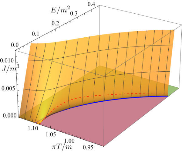

Notably, at , the red dashed curve ends at the point () below the critical embedding (shown by the endpoint of the blue curve: ). This agrees with the phase structure in the D3-D7 model with Mateos:2007vn. That is, the black hole embedding can be found below the value of at the critical embedding. This can be confirmed from the right panel of figure 3. One can find the black hole embedding solutions, which correspond to each point on the green surface in the right panel of figure 3, below . If the brane configuration is the black hole embedding in the absence of the electric field, applying the electric field can instantly produce the current. Therefore, in the high-temperature region (), we can observe linear conduction obeying Ohm’s law.
From each – curve (the vertical black curves), the is multivalued with respect to . At first glance, seems to be the two-valued function of in the left panel of figure 3. However, the self-similar behavior around the critical embedding yields more complicated structure. In the vicinity of the critical embedding, we observe that the current density decreases again with electric field. In figure 4, for instance, we show the behavior near the critical embedding at . For later convenience, we specify the first and second turning point values and , respectively, as denoted by the vertical dashed line in figure 4.
As shown in figure 4, the second turning point in the – curve appears for a small value of . Although we have checked up to the second turning point within numerical accuracy, we expect that this turning structure will appear repeatedly in the vicinity of the critical embedding.
2.4 Effective temperature
In the presence of the electric field, the dynamics of the D7-brane are governed by the effective metric (16). The surface gravity on the effective horizon is defined by
| (17) |
In the middle expression, the minus sign comes from . Then, one can define the effective Hawking temperature as . Figure 5 depicts the plot of with respect to and .
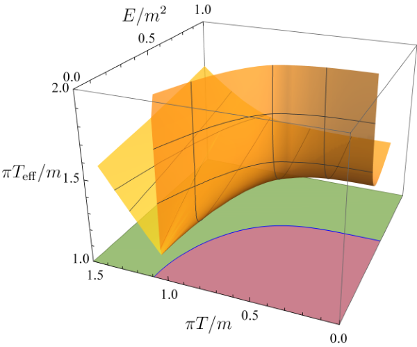
To interpret the behavior of the effective temperature, we solve eq. (14) with respect to and obtain
| (18) |
Because both the numerator and denominator of become zero simultaneously in the limit of , is given by applying L’Hospital’s rule,
| (19) |
At low temperature, in the critical embedding, the current density, , becomes zero, whereas the electric field, , remains a finite value, which corresponds to from eq. (15). Thus, with finite , and the effective temperature diverges at the critical embedding (figure 5). Meanwhile, at high temperature, if we can take the limit of (identical to ) in the black hole embedding, we obtain
| (20) | |||||
where we used in the limit of . Therefore, we confirm that , i.e., the effective temperature becomes identical to the heat bath temperature at . In figure 5, we can see this behavior in the linear conduction regime at high temperatures. As a result, the effective temperature clearly shows the qualitative difference between dielectric breakdown and linear conduction.
3 Linear perturbations
In this section, we formulate linear perturbations on the probe D7-brane. The general ansatz for perturbations of the embedding functions and the worldvolume gauge fields on the D-brane is given by
where and are background solutions, and is a small bookkeeping parameter. Expanding the DBI action to quadratic order in , we obtain the effective action77 7 See appendix A in ref. Mas:2008jz. Eq. (A.9) is the corresponding Lagrangian density. for the perturbations as follows:
| (21) |
where
| (22a) | ||||
| (22b) | ||||
and . Notably, is defined by the inverse of such that is satisfied.
For our purpose of studying the linear stability of the multivalued background profile, we consider the following ansatz for perturbed fields:
| (23) | ||||
where is perpendicular to the -direction. We have assumed that the perturbations do not depend on the -coordinate parallel to the background electric field and current.88 8 When depends on , we have to contain the perturbation field , additionally. Because any other perturbations are decoupled from the above perturbations, we can set the other perturbations to zero without loss of generality. Thus, the quadratic action can be expressed as follows:
| (24) |
where and denote coefficient matrices. Each component of the matrices is given by eqs. (46). The indices denote coordinates . We have written the perturbations as in the above equation. Considering the Fourier transformation with respect to and , we can rewrite as follows:
| (25) |
where . The Fourier components of the perturbations depend on because the background system is isotropic in the -space. Because our system and the background solutions are static and homogeneous, we can rewrite the quadratic action in the momentum space. Writing , we obtain the quadratic action as follows:
| (26) | ||||
where
| (27a) | |||
| (27b) | |||
| (27c) | |||
We have defined
| (28) |
and given by eq. (9). Notably, denotes the inverse of the effective metric (16), which is identical to . In the present case we have and . Hereinafter, we simply write as . denotes each component of with . For convenience, we introduce a new variable by
| (29) |
to remove the factors of non-normalizable modes, , from the perturbations in the vicinity of the AdS boundary. We also write the coefficient matrices for as follows:
| (30a) | ||||
| (30b) | ||||
| (30c) | ||||
Then, the quadratic action for is given by the same form as eq. (26). The equations of motion derived from the action are written as follows:
| (31) |
We solve eq. (31) with proper boundary conditions in the context of the AdS/CFT correspondence. As mentioned in the previous section, the effective horizon is located at on the brane’s worldvolume in the conducting phase. Because the effective horizon is a characteristic surface for the perturbation equations, an ingoing-wave boundary condition should be imposed to study the responses to perturbations.99 9 This choice of the boundary condition in the NESS setup has been employed and discussed in refs. Mas:2009wf; Ishigaki:2020coe; Ishigaki:2020vtr At the effective horizon, we have , so that is a singular point for the perturbation equations. We consider the Frobenius expansion at , as follows:
| (32) |
where denotes a regular function at and is a constant. Substituting eq. (32) into eq. (31), we obtain the characteristic equation for :
| (33) |
where
| (34) |
In the above equations, all functions are evaluated at . Solving the equation for , we find four roots:
| (35) |
where the former one is a double root of the characteristic equation. In the above equation for , we have used the relation between and defined by eq. (17), as follows:
| (36) |
A choice of corresponds to the ingoing-wave solutions in our setup.1010 10 This implies that the coordinates take a form of ingoing Eddington-Finkelstein like coordinates at the effective horizon. To assess this simply, we should consider the high-frequency limit. For sufficiently large , we can drop the second term for in eq. (35), and then and reduce to the Frobenius exponents for the perturbation of the gauge field transverse to in the same background obtained in ref. Ishigaki:2020coe. In that case, the transverse perturbation is decoupled from any other perturbations. It is easy to show that and correspond to the ingoing- and outgoing-wave solutions in the tortoise coordinate of the effective metric, respectively. (See appendix B of ref. Ishigaki:2020coe.) Thus, is expected to be the ingoing-wave solutions in eq. (35), too. More rigorous derivation of the ingoing-wave conditions for our system is presented in appendix B.
We are interested in the stability of this system when we allow fluctuations in the current for a fixed electric field. For this purpose, we should explore the modes of the perturbations satisfying boundary conditions such that non-normalizable modes and outgoing-wave solutions vanish at the AdS boundary () and effective horizon (), respectively. Therefore, by setting , we will determine solutions with a mode frequency by imposing the conditions
| (37) |
where represents a pair of some constant values. The determinant method Amado:2009ts; Kaminski:2009dh helps us find eigenfrequencies and eigensolutions for such a problem. We consider for the given and a set of linearly-independent, ingoing-wave solutions labeled by . In our computation, we set without loss of generality. We can construct a matrix as follows:
| (38) |
which provides . Since is required at the AdS boundary, the mode frequency can be determined by the equation
| (39) |
and the mode functions are determined by solving , meaning that is an eigenvector for with eigenvalue . Meanwhile, if , we write an ingoing-wave solution as follows:
| (40) |
where matrix is a bulk-to-boundary propagator related to a matrix :
| (41) |
In the sense of the field theory, the frequencies of the modes correspond to the poles of Green’s functions. The retarded Green’s function in the NESS can be computed by1111 11 Precisely, we must consider another term from a counterterm of the action Karch:2005ms. The counterterm is needed to regulate the action at the AdS boundary. However, we can ignore it for our purpose to find QNMs.
| (42) |
As mentioned above, is ill-defined when eq. (39) is satisfied, implying that the frequencies satisfying eq. (39) equal the poles of (42). Studying the Green’s function in the NESS is also interesting, but we focus on the poles of the Green’s function in this study.

Figure 6 shows the argument of defined by eq. (39) as a complex function in the complex plane for a background solution. From this figure, one can read mode frequencies, i.e., poles of the Green’s function. According to the determinant method, the poles are located where , corresponding to the intersections of the lines of and in figure 6.
4 Dynamical stability in the conducting phase
In this section, we describe the dynamical stability of our system in the conducting phase. From section 2, multiple solutions with various emerge for a given electric field, , or temperature, , in the conducting phase. The stability of our system can be investigated by solving the perturbation equations. We find instability associated with the multivalued property of the – curves in the system. Further, there are static solutions of the perturbation fields with a specific spatial scale, implying that the system also has an inhomogeneous background solution.
4.1 Stability for homogeneous perturbations and multivaluedness
4.1.1 Zero temperature
First, we show the behavior of the mode frequencies with respect to homogeneous perturbations of and at zero temperature with a finite current. As shown in the left panel of figure 4, two branches in the background solutions appear for ; for a given electric field, the upper (lower) branch has a higher (lower) electric current than . In figure 7 we show some frequencies of the QNMs, i.e., the poles of the retarded Green’s functions, in the complex plane. The left and right panels correspond to background solutions with on the upper branch and a background solution with on the lower branch, respectively. We find that, in the left panel (the upper branch), no pole locates in the upper-half plane of , whereas, in the right panel (the lower branch), a pole on the imaginary axis, , has moved to the upper-half plane of . In fact, it turns out that this pure-imaginary mode is the first going across the real axis at the turning point as decreases from the upper to lower branch.1212 12 From the left panel of figure 7, one can find poles at . In this figure, these poles have very small negative imaginary part. We have checked these poles also locate on the lower-half plane when the background solution is the upper branch solution. Figure 8 shows of the pure-imaginary mode as a function of around the first turning point. Thus, we conclude that the upper branch solutions with higher are stable, whereas the lower branch ones with lower become unstable against the corresponding linear perturbations.
In addition, we observe the asymptotic behavior of the pure-imaginary mode for large . Figure 9 shows as a function of . We find that this mode locates on the imaginary axis for any , and seems to converge to in the limit of . In the massless quark case, i.e., , the current is analytically given by . This asymptotic value equals for , where denotes the surface gravity on the effective horizon defined in eq. (17).1313 13 An equation of motion for the perturbation of the embedding function in the case of massless quark and applying has been derived in ref. Albash:2007bq.
Then, we also examine the behavior of poles around the second turning point of the – curve at , shown in the right panel of figure 4. The second turning point is located at . We show mode frequencies on the complex plane for and in figure 10. We will refer to a set of solutions within as the (second) upper branch, and a set of solutions with as the (second) lower branch. The left and right panels of figure 10 correspond to solutions of the (second) upper and lower branches in the right panel of figure 4, respectively. Notably, there exists one more branch with a higher , which is represented in the left panel of figure 4. Because the – curve has already been multivalued for a given in , both branches extending from the second turning point have an unstable mode on the imaginary axis, as seen previously.
In the left panel (), we find two poles near the origin of in the lower-half plane; so, these are stable modes. Meanwhile, in the right panel (), the corresponding poles become two pure-imaginary modes newly added on the imaginary axis, one of which is located in the upper-half plane and is unstable. To illustrate the behavior of the two poles, we show of these poles as functions of in figure 11. As decreases, these two poles first approach each other in the lower-half plane to meet on the imaginary axis and then move apart on the imaginary axis. We find that the second turning point corresponds to for one of these poles.
At the first and second turning points of the – curve, we observed a pole with . It seems to be quite natural for the following reasons. At a turning point of the – curve, the background solution will bifurcate into two branches with different for a given , implying a static perturbation to an infinitesimally change of for a fixed . Moreover, the results agree with an expectation that is related to the retarded Green’s function by the Green-Kubo formula, even in the NESS. The divergence of corresponds to the existence of a pole at zero. We expect that a pole with corresponding to a static perturbation will emerge at every other turning point.
4.1.2 Finite temperature
We now proceed to study the dynamical stability at a finite temperature. We focus only on a pure-imaginary mode because this mode will govern the stability of the system.
The relation between the instability and the multivalued property of the – curves is more clearly illustrated in figure 12. It shows the – curves and the relation between and the imaginary part of mode frequency for the pure-imaginary mode at various temperatures. In the vicinity of the critical electric field or small-current region, becomes a multivalued function of . In the multi-valued region, there are mostly two branches of background solutions: the upper branches with higher and lower branches with lower for the given and . We observe that is negative and positive throughout the upper and lower branches, respectively. The zero-points of completely match the line of the first turning points in the – curves (figure 12). These results imply that the lower branches are unstable against homogeneous perturbations of the current or quark condensate.
4.2 Inhomogeneous perturbations: spatial instability
Now, we consider inhomogeneous perturbations with finite wavenumber perpendicular to the electric field and current. As mentioned above, in the multivalued region near the critical electric fields the background solutions of the lower- branch have instability, resulting from the pure-imaginary mode for the homogeneous perturbations. Figure 13 shows the imaginary part of frequency for the pure-imaginary mode as functions of for several points on the – curve at . Because means the homogeneous perturbations, the electric currents , , and represent an unstable solution on the lower branch, marginal one on the turning point, and stable one on the upper branch, respectively. We observe decreases as increases for each . In particular, can go across zero at a specific wavenumber even if is positive at , i.e., the homogeneous perturbation is a growing mode, meaning that our system becomes unstable against perturbations below a critical wavenumber, and this instability is a long-wavelength instability. We can find such for the background solutions on the lower branch which has positive when . Because the perturbative solution can be both static and inhomogeneous with a specific length scale, , the existence of implies that the system also has inhomogeneous nonlinear solutions such that the current density is spatially modulated (figure 1).
Figure 14 shows relations between and at various temperatures. For , becomes multivalued to because there are two unstable solutions for given in the – curves. The endpoints where correspond to the first turning points for each temperature (figure 15). In the vicinity of , blows up, meaning that this instability will extend to any short length-scale toward the critical embedding solutions.
We also show relations between and in figure 16, where we have plotted as functions of in log-log scale at various temperatures. From this figure, behaves as a power function of for each temperature. We also read the power-law index in the vicinity of by a linear fitting. If we write the relation in the vicinity of as
| (43) |
where and are constant, the exponents at various temperatures are estimated as follows:
| (44) |
These values are estimated from the data around small but finite . We expect that the true exponent will be given by for any temperature.
5 Conclusion and discussion
In this article, we study the D3-D7 model under an electric field. We focus on the NESS system with a constant current in the dual field theory. Moreover, we perform a linear stability analysis of the background states.
In section 2, we present the phase diagram of the conducting/insulating phases and the behaviors of the current density, quark condensate, and effective temperature as functions of and . Figure 3 shows the multivalued with respect to for various . On decreasing or , we find the first turning point in the – curves. At smaller , we also find the second turning point (figure 4). At , a similar multivaluedness of the parameters in the D3-D7 model has been found in refs. Mateos:2006nu; Mateos:2007vn; Frolov:2006tc. We expect that the turning points will repeatedly appear in the – curves until reaching . This behavior of the probe brane system in the black hole geometry may be understood as the discrete scale invariance Sornette_1998. Similar behaviors could be observed experimentally in an insulator in the vicinity of the electric breakdown.
To study the linear stability of the system, we consider the current perturbation of the background solution in the multivalued region. On the gravity side, this corresponds to the perturbation of the worldvolume gauge field parallel to the external electric field being coupled with the perturbation of the brane embedding. By solving the equations for the coupled perturbations and computing the QNMs, we find the dynamical instability of the NESS system in the multivalued region. At any temperature, the upper and lower branches of the – curves are, respectively, stable and unstable against the homogeneous perturbations.
The authors of Kaminski:2009ce showed similar observations in the D3-D7 model without applying , i.e., an equilibrium system. In equilibrium, the on-shell action of the probe brane is regarded as a thermodynamic potential of the boundary theory Mateos:2006nu; Mateos:2007vn. It has also been shown that solutions corresponding to the unstable branch of the thermodynamic potential are dynamically unstable from the QNM analysis. On the unstable branch, the quark condensate is multivalued for a given quark mass. Their unstable solutions with vanishing density correspond to our unstable solutions in the limit of . So far, in this study, we focus on the dynamical stability of the system with respect to small perturbations. It is also intriguing to consider about thermodynamic stability of the NESS. If we can define a meaningful “thermodynamic potential,” even for the NESS system, it might show a swallow-tail structure for and determine the first-order transition point. Our results indicate the dynamical instability of the NESS system, but the thermodynamic stability is uncertain.
By considering the finite wavenumber for the perturbations around an unstable branch, we find the critical wavenumber with which the perturbations do not depend on time, meaning the background solution with the static perturbation, which has the specific scale of the critical wavelength, can be realized. It also implies that there are inhomogeneous background states as new branches around the unstable solutions. Current filaments can be realized in conductors that show negative differential conductivity Schoell:2001. We expect that our observations indicate the holographic realization of the current filaments. Notably, the perturbation becomes unstable in the long-wavelength region (figure 13). Because the unstable modes do not appear in the system with the finite size , it is expected that a homogeneous state also becomes stable. In addition, we remark that the direction of the inhomogeneity is symmetric under the rotation in - plane because the system is isotropic in this plane. Assuming that the phase transition from a homogeneous state to an inhomogeneous state occurs, the rotational symmetry will be spontaneously broken, or explicitly broken by perturbing along a specific direction.
Several open questions should be explored in the future. First, the relation between dynamical and thermodynamic stabilities in the NESS system should be examined. Holographically, a naive candidate for the ‘‘thermodynamic potential’’ in the NESS system might be the probe brane action as in equilibrium.1414 14 For example, the authors of Matsumoto:2018ukk; Imaizumi:2019byu studied the several critical exponents by using the on-shell DBI action as the thermodynamic potential under the same setup of the NESS system. A similar definition was also given in Banerjee:2015cvy. It would be interesting to compare our results with the “thermodynamic potential” in the same parameter region.
Another direction is to find inhomogeneous nonlinear solutions, which are indicated by our linear stability analysis, apart from the linear perturbation analysis. To do this, one must solve the nonlinear partial differential equations as the equations of motion for the fields in the D3-D7 model. Thus, one can investigate the stability of the inhomogeneous solutions.
It would be crucial to understand the origin of the dynamical instability in our setup. The authors of Nakamura:2009tf found a filamentary instability by considering a five-dimensional Maxwell theory with the Chern-Simons (CS) term in AdS spacetime. A similar instability has been observed in the D3-D7’ model which duals to the gauge field theory with quark-like particles in -dimensions by the authors of Bergman:2011rf. In both cases, the considered system becomes dynamically unstable at a specific finite range of the wavenumber, unlike our case. This type of filamentary instability originated from the CS term in the gravity model action. In our system, because the CS term does not affect the perturbations in the linear order, the filamentary instability must have another origin. This is left for future work.
Acknowledgements.
The authors are grateful to Shin Nakamura and Yuichi Fukazawa for the fruitful discussion. S. I. is supported by National Natural Science Foundation of China with Grant No. 12147158. M. M. is supported by National Natural Science Foundation of China with Grant No. 12047538. S. K. is supported by JSPS KAKENHI Grant Numbers JP16K17704, JP21H05189. The authors thank RIKEN iTHEMS NEW working group for fruitful discussions. The authors would like to thank Enago (www.enago.jp) for the English language review.Appendix A Numerical details
In this study, we have mainly used a shooting method for computing the QNMs. To solve eq. (31) numerically, we need to introduce a small cutoff around the singularities of the differential equations at and . Thus, the integral region becomes where are numerical cutoffs. With the ingoing-wave boundary condition, we can obtain a series solution for the perturbation fields around . We can solve eq. (31) numerically by imposing a condition at which claims that the numerical solution equals the series solution at this point. In our computation, we used and the series solution up to the first order of .
The authors of Kaminski:2009ce pointed out that the shooting method could be difficult for computing QNMs with large . Because we focus on the QNMs with small , we expect to avoid the difficulty. To ensure this, we attempted to use a relaxation method for computing the QNMs. In the relaxation method, we discretized the equations of motion with the second-order finite differences on the grid points. Using an appropriate initial configuration, we obtained the numerical solutions after iteration in the Newton-Raphson relaxation scheme. We stopped the iteration when the root mean squared error with respect to the equations of motion was less than . We also checked the convergence of the variables with respect to the number of grid points. The discretization error in the second-order differences was expected to be given by the square of the grid size. Thus, if we double the grid points to , the discretization error should be reduced to a quarter of that in grid points. Figure 17 shows the typical convergence behavior of with respect to the number of grid points . We define the numerical error as , where is the numerical value of the quasinormal frequency with grid points.
Figure 17 indicates that the numerical error converges as the number of grid points increases. For , the numerical error converges as , which roughly agrees with that expected from the discretization error, namely . Moreover, because the convergence is not improved for , the improvement of the numerical accuracy is also unexpected for more grid points. Notably, the background solutions and , which are also numerically obtained, may affect the numerical error of the relaxation method. The convergent behavior of the quantity with respect to the grid points implies that the numerical scheme works well for our problem.
We show the comparison of the shooting and relaxation method and the relaxation in figure 18. We plot as a function of at using two different methods. The data of the shooting method are the same as in figure 12 and figure 14. The results computed from the two methods almost agree with each others. Consequently, our results in the shooting method do not encounter the difficulty discussed in ref. Kaminski:2009ce.
Appendix B Ingoing-wave boundary condition
We now discuss the ingoing-wave boundary condition from the effective action of the perturbations in the position space. It is given by
| (45) |
with coefficient matrices:
| (46a) | |||
| (46b) | |||
where
| (47a) | |||
| (47b) | |||
is defined by eq. (28). is a symmetric matrix, and is an antisymmetric matrix. satisfies by definition. is diagonalized as
| (48) |
with an orthogonal matrix
| (49) |
In the above equations, we have defined
| (50) |
We write . and are real because is a real symmetric matrix. under the transformation because it is a totally antisymmetric matrix.
Because we are interested in the behavior of the fields in the vicinity of the effective horizon, we can treat all coefficients as constants evaluated at except which vanishes at . Then, we can partially decouple the fields by introducing new fields: where . We also define as an inverse matrix of . In (45), relevant terms to the field behavior in the vicinity of , are only the derivative terms. Then, the action with relevant terms is given by
| (51) |
where denotes the antisymmetric part of which is given by
| (52) |
We ignored the symmetric part of and the term with by integration by parts. Now, we introduce the tortoise coordinates of the effective metric:
| (53) |
In these coordinates, a relevant part of the first term in (51) is given by
| (54) |
A relevant contribution from the second term in (51) is given by
| (55) | ||||
Notably, we can write , and is defined in eq. (34). We obtain
| (56) |
where denotes terms of in the vicinity of the effective horizon.1515 15 Be aware that because is negative.
Finally, we rewrite the fields as a complex field, as follows:
| (57) |
In terms of , the relevant part of the action is written as a simple form:
| (58) |
Therefore, the equation of motion for is given by
| (59) |
We write solutions of the equation of motion and its complex conjugate, respectively, as1616 16 We can also write .
| (60) |
In the vicinity of the effective horizon, the relation between the tortoise coordinates and - coordinates is given by
| (61) |
where we have used eq. (36) for rewriting which is the surface gravity on the effective horizon defined by eq. (17). Because corresponds to , a choice of the positive/negative sign in (60) corresponds to the outgoing/ingoing-wave solution at the effective horizon. In terms of , the real field is written as
| (62) | ||||
in the vicinity of where
| (63) | ||||
for . We can also obtain a similar result for . The original fields are given by linear combinations of . The four exponents of (63) completely match to those of (35). Consequently, we can understand that for corresponds to the set of the ingoing-wave solutions manifestly because the negative sign has been taken in eq. (60).
References
- (1) J.M. Maldacena, The large N limit of superconformal field theories and supergravity, Adv. Theor. Math. Phys. 2 (1998) 231 [hep-th/9711200].
- (2) S.S. Gubser, I.R. Klebanov and A.M. Polyakov, Gauge theory correlators from non-critical string theory, Phys. Lett. B 428 (1998) [hep-th/9802109].
- (3) E. Witten, Anti-de sitter space and holography, Adv. Theor. Math. Phys. 2 (1998) [hep-th/9802150].
- (4) H. Liu and J. Sonner, Holographic systems far from equilibrium: a review, 1810.02367.
- (5) A. Karch and E. Katz, Adding flavor to AdS / CFT, JHEP 06 (2002) 043 [hep-th/0205236].
- (6) A. Karch and A. O’Bannon, Metallic AdS/CFT, JHEP 09 (2007) 024 [0705.3870].
- (7) J. Erdmenger, R. Meyer and J.P. Shock, AdS/CFT with flavour in electric and magnetic Kalb-Ramond fields, JHEP 12 (2007) 091 [0709.1551].
- (8) T. Albash, V.G. Filev, C.V. Johnson and A. Kundu, Quarks in an external electric field in finite temperature large N gauge theory, JHEP 08 (2008) 092 [0709.1554].
- (9) O. Bergman, G. Lifschytz and M. Lippert, Response of Holographic QCD to Electric and Magnetic Fields, JHEP 05 (2008) 007 [0802.3720].
- (10) K. Hashimoto and T. Oka, Vacuum Instability in Electric Fields via AdS/CFT: Euler-Heisenberg Lagrangian and Planckian Thermalization, JHEP 10 (2013) 116 [1307.7423].
- (11) S. Nakamura, Negative Differential Resistivity from Holography, Prog. Theor. Phys. 124 (2010) 1105 [1006.4105].
- (12) D. Mateos, R.C. Myers and R.M. Thomson, Thermodynamics of the brane, JHEP 05 (2007) 067 [hep-th/0701132].
- (13) M. Kaminski, K. Landsteiner, F. Pena-Benitez, J. Erdmenger, C. Greubel and P. Kerner, Quasinormal modes of massive charged flavor branes, JHEP 03 (2010) 117 [0911.3544].
- (14) G.T. Horowitz and V.E. Hubeny, Quasinormal modes of AdS black holes and the approach to thermal equilibrium, Phys. Rev. D 62 (2000) 024027 [hep-th/9909056].
- (15) A. Nunez and A.O. Starinets, AdS / CFT correspondence, quasinormal modes, and thermal correlators in N=4 SYM, Phys. Rev. D 67 (2003) 124013 [hep-th/0302026].
- (16) P.K. Kovtun and A.O. Starinets, Quasinormal modes and holography, Phys. Rev. D 72 (2005) 086009 [hep-th/0506184].
- (17) M. Kaminski, K. Landsteiner, J. Mas, J.P. Shock and J. Tarrio, Holographic Operator Mixing and Quasinormal Modes on the Brane, JHEP 02 (2010) 021 [0911.3610].
- (18) E. Schöll, Nonlinear Spatio-Temporal Dynamics and Chaos in Semiconductors, Cambridge University Press (2001).
- (19) K. Hashimoto, S. Kinoshita, K. Murata and T. Oka, Electric Field Quench in AdS/CFT, JHEP 09 (2014) 126 [1407.0798].
- (20) K.-Y. Kim, J.P. Shock and J. Tarrio, The open string membrane paradigm with external electromagnetic fields, JHEP 06 (2011) 017 [1103.4581].
- (21) N. Seiberg and E. Witten, String theory and noncommutative geometry, JHEP 09 (1999) 032 [hep-th/9908142].
- (22) D. Mateos, R.C. Myers and R.M. Thomson, Holographic phase transitions with fundamental matter, Phys. Rev. Lett. 97 (2006) 091601 [hep-th/0605046].
- (23) V.P. Frolov, Merger Transitions in Brane-Black-Hole Systems: Criticality, Scaling, and Self-Similarity, Phys. Rev. D 74 (2006) 044006 [gr-qc/0604114].
- (24) M. Kruczenski, D. Mateos, R.C. Myers and D.J. Winters, Meson spectroscopy in AdS / CFT with flavor, JHEP 07 (2003) 049 [hep-th/0304032].
- (25) I. Kirsch, Spectroscopy of fermionic operators in AdS/CFT, JHEP 09 (2006) 052 [hep-th/0607205].
- (26) R. Abt, J. Erdmenger, N. Evans and K.S. Rigatos, Light composite fermions from holography, JHEP 11 (2019) 160 [1907.09489].
- (27) K. Hashimoto, S. Kinoshita and K. Murata, Conic D-branes, PTEP 2015 (2015) 083B04 [1505.04506].
- (28) J. Mas, J.P. Shock, J. Tarrio and D. Zoakos, Holographic Spectral Functions at Finite Baryon Density, JHEP 09 (2008) 009 [0805.2601].
- (29) J. Mas, J.P. Shock and J. Tarrio, Holographic Spectral Functions in Metallic AdS/CFT, JHEP 09 (2009) 032 [0904.3905].
- (30) S. Ishigaki and S. Nakamura, Mechanism for negative differential conductivity in holographic conductors, JHEP 12 (2020) 124 [2008.00904].
- (31) S. Ishigaki and M. Matsumoto, Nambu-Goldstone modes in non-equilibrium systems from AdS/CFT correspondence, JHEP 04 (2021) 040 [2012.01177].
- (32) I. Amado, M. Kaminski and K. Landsteiner, Hydrodynamics of Holographic Superconductors, JHEP 05 (2009) 021 [0903.2209].
- (33) A. Karch, A. O’Bannon and K. Skenderis, Holographic renormalization of probe D-branes in AdS/CFT, JHEP 04 (2006) 015 [hep-th/0512125].
- (34) D. Sornette, Discrete-scale invariance and complex dimensions, Physics Reports 297 (1998) 239–270.
- (35) M. Matsumoto and S. Nakamura, Critical Exponents of Nonequilibrium Phase Transitions in AdS/CFT Correspondence, Phys. Rev. D 98 (2018) 106027 [1804.10124].
- (36) T. Imaizumi, M. Matsumoto and S. Nakamura, Current Driven Tricritical Point in Large- Gauge Theory, Phys. Rev. Lett. 124 (2020) 191603 [1911.06262].
- (37) A. Banerjee, A. Kundu and S. Kundu, Flavour Fields in Steady State: Stress Tensor and Free Energy, JHEP 02 (2016) 102 [1512.05472].
- (38) S. Nakamura, H. Ooguri and C.-S. Park, Gravity Dual of Spatially Modulated Phase, Phys. Rev. D 81 (2010) 044018 [0911.0679].
- (39) O. Bergman, N. Jokela, G. Lifschytz and M. Lippert, Striped instability of a holographic Fermi-like liquid, JHEP 10 (2011) 034 [1106.3883].