Regularization from examples via neural networks for parametric inverse problems: topology matters

In inverse problems, Neural Networks (NNs) have been used in many different contexts: i) to approximate a suitable penalty term in Tikhonov–like regularization approaches; ii) to estimate the value of the regularization parameter; iii) to replace time–consuming operations in unrolled schemes; iv) to post–process coarse reconstructions; and v) to directly approximate an inverse regularizing operator. We refer the reader to [4, 14, 18] and references therein for a recent overview.

In this paper we are interested in the latter strategy, which can bring important advantages with respect to the classical Tikhonov regularization. First, the point-wise solution of the inverse problem is obtained by simply applying the trained NN to the assigned data. This is possible thanks to the fact that solving an inverse problem by using a NN yields a local solution, valid in a neighborhood of the data examined in the training set. Indeed, the biggest computational effort is spent during the network optimization phase which takes place independently of the knowledge of the assigned data of the inverse problem. Second, deep approximation techniques are not limited to the treatment of linear inverse problems, but can be easily extended to the case of non–linear ones [2]. In this work, we focus on parametric inverse problems, where the solution is described by a finite number of parameters. Although there is some literature that deals with either approximating the inverse operator [3, 26, 25], or estimating the parameters of interest [13, 8], by means of NNs, little attention has been paid to the regularization properties of the provided inversion method. Specifically, as a regularizing inverse operator must be continuous with respect to the data, topological issues could arise when predicting the parameters directly with a NN. For instance, let us consider the problem of mapping the points of $\mathbb{S}^{1}$ into the corresponding angle $\theta$. In this case, data close to $(1,0)$ would be mapped either close to $0$ or to $2\pi$, thus producing a discontinuity if the Euclidean topology is considered on the angle space. Hence, this map can not be accurately approximated by a NN as the latter is a continuous function when both the domain and the codomain are equipped with the Euclidean topology. This simple example suggests that the naive approach based on using a NN to map the data directly into the parameters may lead to suboptimal results in practice.

We provide a general treatment for the solution of parametric inverse problems when a dataset of parameter–data pairs is available. The contribution of the paper is twofold. First, under mild conditions on the forward operator, we derive the correct topology of the parameter space needed for defining a regularizing operator. Second, we describe a strategy for approximating the regularizing operator with NNs. This strategy relies on the knowledge of an embedding of the parameter space into a (low–dimensional) Euclidean one. Then, a NN is used for approximating a homeomorphism between the image of the parameter space through the forward operator and the embedded space. Finally, the parameters are retrieved by applying the inverse of the embedding to the neural network predictions. The advantage of this approach is that the network is used for approximating a continuous function between Euclidean spaces, in this way avoiding the discontinuity issues that arise when a NN is used to map non-homeomorphic spaces.

We demonstrate the effectiveness of the proposed method on a parametric imaging problem from synthetic data of the Spectrometer/Telescope for Imaging X-rays (STIX) [12], the X-ray telescope of the Solar Orbiter mission. In particular, we show that, when a specific shape is used for parameterizing the solution of the inverse problem, the parameter space has a topology strictly coarser than the Euclidean one that makes it homeomorphic to a family of Moebius strips that collapse into a point. In this context, our proposed strategy clearly outperforms the naive approach, which does not take into account the topology of the parameter space.

The reminder of the paper is organized as follows. In Section 2 we describe the mathematical formulation of the parametric regularization and we provide details about the topology that has to be considered on the parameter space for defining a regularizing operator. Section 3 is devoted to the treatment of topological issues arising when the parameter space is not endowed with the Euclidean topology and the regularizing operator is approximated directly with a NN. Further, we describe the proposed strategy for overcoming these issues. In Section 4 we present the image reconstruction problem for STIX and the parametric shape used for approximating the solution. Finally, the results of the numerical experiments are shown in Section 5. Section 6 is devoted to conclusions.

In the context of this paper, the data space is $\mathbb{R}^{M}$ endowed with the Euclidean topology $\varepsilon$. The object space $\mathcal{H}$ is a function space equipped with the coarsest topology $\eta$ that makes continuous the (possibly non-linear) operator $\mathcal{A}\colon\mathcal{H}\to\mathbb{R}^{M}$ modeling the data formation and acquisition process. Our problem is then the ill–posed inverse problem of finding an object $f\in\mathcal{H}$ that satisfies

where $g$ is the experimental data corrupted by noise. We propose to seek for a regularized solution into a parametric subspace of $\mathcal{H}$. With this in mind, we assume that the exact solution $f^{\ast}$ belongs to a subset defined as the image of a function $\Phi\colon\Theta\to\mathcal{H}$, where $\Theta$ is a subset of $\mathbb{R}^{P}$ with non–empty interior called parameter space. We denote by $\varepsilon_{\Theta}$ the subspace topology induced on $\Theta$ by the Euclidean topology of $\mathbb{R}^{P}$ and we assume that $\Phi$ is continuous on $(\Theta,\varepsilon_{\Theta})$. We can then recast the ill–posed inverse problem (1) as the one of finding $\theta$ such that

Hereafter, we will denote with $\mathcal{M}$ the noise–free data subset, i.e. $\mathcal{M}\mathrel{\vbox{\hbox{$:$}}{=}}(\mathcal{A}\circ\Phi)(\Theta)$, and we will equip $\mathcal{M}$ with the topology $\varepsilon_{\mathcal{M}}$ inherited as a subspace of $\mathbb{R}^{M}$.

We can define a continuous inverse of $\mathcal{A}\circ\Phi$ on $\mathcal{M}$ provided that the following two conditions hold:

• $(i)$

  $\mathcal{A}\circ\Phi$ is injective;

• $(ii)$

  we consider on $\Theta$ the coarsest topology that makes continuous $\mathcal{A}\circ\Phi$, i.e.

  $$\tau\mathrel{\vbox{\hbox{$:$}}{=}}\left\{(\mathcal{A}\circ\Phi)^{-1}(\mathcal{U})~\colon~\mathcal{U}\in\varepsilon_{\mathcal{M}}\right\}~.$$

  (3)

These conditions are crucial to define a regularizing operator. Indeed, the topology $\tau$ makes continuous also the inverse of $\mathcal{A}\circ\Phi$ on $\mathcal{M}$, as proved in the following Lemma.

In this section, we show how to construct an approximation of the regularizing operator $\mathcal{R}$ by means of a dataset of examples, i.e. a set of pairs $\{(g_{i},\theta_{i})\}_{i=1}^{S}$ with $\theta_{i}\in\Theta$ and $g_{i}\approx(\mathcal{A}\circ\Phi)(\theta_{i})\in\mathbb{R}^{M}$, representing a noisy sampling of the graph of $\mathcal{A}\circ\Phi$. Towards this aim, we make use of NNs [7, 10], which are simply parametric functions obtained by recursively composing a certain number of layers. Each layer is defined as $l_{W,b}(z)\mathrel{\vbox{\hbox{$:$}}{=}}\sigma(Wz+b)$, where $z\in\mathbb{R}^{n}$ is the input, $W\in\mathbb{R}^{m\times n}$ is the weight matrix, $b\in\mathbb{R}^{m}$ is the bias and $\sigma\colon\mathbb{R}\to\mathbb{R}$ is a continuous non-linear function (called activation function) applied component-wise. A NN is then a function $\mathcal{N}_{\mathcal{W}}$ of the form

where $L>1$ is the number of layers and $\mathcal{W}$ is the set of the network weights (the entries of the weight matrices and of the biases). A function defined as in (5) is then trained to perform a task, i.e. the weights are modified by means of an optimization procedure so that it approximates a given function.

A straightforward application consists in training a NN to predict the parameter $\theta$ from the corresponding $g$ by solving

By doing so, $\mathcal{N}_{\mathcal{W}^{\ast}}$ is an approximation of $\mathcal{R}$ that is continuous w.r.t. the Euclidean topology considered both in the domain and in the codomain. Indeed, any NN of the form (5) is implicitly defined from $\mathbb{R}^{n}$ in $\mathbb{R}^{m}$ as Euclidean spaces. However, if the topology $\tau$ on $\Theta$ is strictly coarser than $\varepsilon_{\Theta}$, as we previously discussed, the NN should be discontinuous for providing a good approximation of $\mathcal{R}$, leading to an evident contradiction.

To show the issues that arise when applying this naive approximation of $\mathcal{R}$ with a NN, we consider again Example 2.1. By using $S=30000$ samples drawn at random from the set $\Theta$, i.e. $\theta_{i}$ for $i=1,\ldots,S$ and their corresponding values $g_{i}=(\cos\theta_{i},\sin\theta_{i})$, we train a NN $\mathcal{N}$ approximating $\mathcal{R}$ by solving (6). In Figure 2 we report the scatter plot of the angle $\theta$ predicted by $\mathcal{N}$ from the point $g=(\cos(\theta),\sin(\theta))\in\mathcal{M}$ over a test set of $200000$ examples. The plot clearly shows that, according to Lemma 2.2, $\mathcal{N}$ approximates a discontinuity in $(1,0)$ in a continuous way, causing a systematic error in a neighborhood of $(1,0)$.

To overcome this drawback, we propose the following strategy. Denoting with $\mathcal{E}$ a subset of $\mathbb{R}^{N}$ and with $\varepsilon_{\mathcal{E}}$ the topology inherited as a subspace of $\mathbb{R}^{N}$, we assume to have an analytical expression of an embedding

and of its inverse $\gamma^{-1}$ over $\mathcal{E}$. In the usual case, $(\Theta,\tau)$ is a smooth manifold and the Whitney embedding theorem [1] guarantees the existence of the embedding and ensures that $N\leq 2P$. Moreover, in practice, $(\Theta,\tau)$ is typically a simple manifold (e.g. a circumference, a sphere, a torus, etc.) for which analytical embeddings in $\mathbb{R}^{N}$ are well known. As $\gamma$ is a homeomorphism, finding a continuous inverse of $\mathcal{A}\circ\Phi$ on $\mathcal{M}$ can be recast as the problem of approximating a homeomorphism $\psi$ between $\mathcal{M}$ and $\mathcal{E}$:

For this approximation task we can make use of a NN, as the topologies in the domain and codomain are induced by the Euclidean one. Then, the training problem looks like

Finally, an approximated regularizing operator for problem (2) can be defined as

Figure 3 offers a schematic of the operators involved in the definition of $\mathcal{R}$. The role of $\gamma^{-1}$ is to map each point of $\mathcal{E}$ into a parameter value $\theta$ in a continuous way w.r.t. the topology $\tau$ and in a discontinuous way w.r.t. $\varepsilon_{\Theta}$. Instead, $\mathcal{N}_{\mathcal{W}^{\ast}}$ is a continuous transformation between $\mathbb{R}^{M}$ and $\mathbb{R}^{N}$, both equipped with the Euclidean topology. When $N\leq M$ (and often in applications $N\ll M$), $\mathcal{N}_{\mathcal{W}^{\ast}}$ performs a dimensionality reduction task. In any case, $\mathcal{N}_{\mathcal{W}^{\ast}}$ is defined and continuous on the entire space $\mathbb{R}^{M}$. Therefore, when the inverse $\gamma^{-1}$ can be continuously extended to a neighborhood containing $\mathcal{E}$, the (approximated) regularizing operator $\mathcal{R}$ is a continuous extension of the left inverse of $\mathcal{A}\circ\Phi$. It is worth noticing that our proposed strategy represents a generalization of the naive approach. Indeed, when the topology $\tau$ coincides with the Euclidean one, we can trivially choose $\gamma$ as the identity function and problem (9) is the same as (6).

In this section we describe the parametric imaging problem for the Spectrometer/Telescope for Imaging X-rays (STIX) [12], an instrument on board the Solar Orbiter satellite launched by the European Space Agency in February 2020. STIX is conceived for the study of solar flares, intense phenomena that arise on the Sun surface. During these events, a sudden release of energy stored in the magnetic field of the Sun accelerates electrons and causes the emission of X-ray photons by bremsstrahlung [6]. The goal of the inverse imaging problem from STIX data is to retrieve the image of the X-ray emission from the measurements of the photons incident on the telescope [15, 16, 17, 20]. STIX exploits a bigrid imaging system that allows the sampling of the Fourier transform of the photon flux in 30 frequencies $\xi_{j}=(u_{j},v_{j})$, $j=1,\dots,30$ [9, 12] (see Figure 4 for a representation). Therefore, the STIX imaging problem can be described by the equation

where $\varphi(x,y)$ is the function representing the number of photons emitted per unit area from the location $(x,y)$ on the Sun surface, $V\in\mathbb{C}^{30}$ is the array containing the experimental values of the Fourier transform called visibilities and $\mathcal{F}$ is the Fourier transform computed in $\xi_{1},\dots,\xi_{30}$ defined by¹¹ 1 Note that the adopted definition of Fourier transform is typical of astronomical applications and differs from the usual one because of a plus sign.

In the following, $\mathbb{C}^{30}$ will be considered as $\mathbb{R}^{60}$.

As the morphology of solar flares is quite simple, the images to reconstruct are usually composed by a few basic geometric shapes such as elliptical Gaussians or loops [5, 21, 22] (Figure 5).

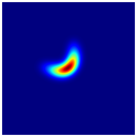
Such shapes are bidimensional functions $\varphi_{\theta}(x,y)$ parameterized by an array $\theta$ containing, for instance, the coordinates of the center of the shape, the eccentricity, the rotation angle, etc. Therefore, in the case of the parametric imaging problem for STIX, the parameterization is the function $\Phi$ that maps $\theta$ into $\varphi_{\theta}$ and problem (11) becomes the one of finding $\theta$ such that

Since the Gaussian elliptical shape is a special case of the loop shape with curvature equal to zero, in the following we will consider $\varphi_{\theta}$ as a loop and we will provide a description of the topology $\tau$ of the parameter space in such a case.

A loop shape is defined by the following parameters (see Figure 6):

• •

  the coordinates $(x_{c},y_{c})$ of the center of the shape;

• •

  the intensity $F$, also named total flux, that is the integral of $\varphi_{\theta}$ over $\mathbb{R}^{2}$;

• •

  the Full Width at Half Maximum (FWHM) $\sigma$, which represents the width of the level curve of the loop at $50$% of the peak;

• •

  the curvature $c$ that describes the bending of the loop;

• •

  the eccentricity $\varepsilon$, that, when the curvature is 0, is related to the eccentricity of the elliptical level curve at half maximum of the shape;

• •

  the rotation angle $\alpha$.

In our case, then, $\theta\mathrel{\vbox{\hbox{$:$}}{=}}(x_{c},y_{c},F,\sigma,\varepsilon,\alpha,c)$. More in detail, as shown in Figure 6, a loop shape is given by a superimposition of circular Gaussian shapes with FWHM equal to $\sigma$ and centers located on a parabola of equation $y=cx^{2}$ rotated of angle $\alpha$. The expression of the loop is then

where $\sum_{j}w_{j}=1$, $w_{j}>0$ decreases for increasing distance of $(x_{j},y_{j})$ with respect to $(x_{c},y_{c})$ and the distance between $(x_{j},y_{j})$ and $(x_{j-1},y_{j-1})$ along the parabola is proportional to $\varepsilon\geq 0$. We point out that when $\varepsilon=0$, the loop shape becomes a circular Gaussian shape that is invariant with respect to rotations of angle $\alpha$ and bending with curvature $c$. In the following, we will set $c=0$ and $\alpha=0$ when $\varepsilon=0$.

The parameter space of this inverse problem is

where $\mathcal{I}_{X}$, $\mathcal{I}_{Y}$, $\mathcal{I}_{F}$ and $\mathcal{I}_{\sigma}$ are the intervals of definition of $x_{c}$, $y_{c}$, $F$ and $\sigma$, respectively, and $\mathcal{I}_{\varepsilon,\alpha,c}\mathrel{\vbox{\hbox{$:$}}{=}}((0,\varepsilon_{\max}]\times[0,180)\times[c_{\min},c_{\max}])\cup\{(0,0,0)\}$.

If we fix $\varepsilon>0$ and all the other parameters but $\alpha$ and $c$, then the parameter space becomes $\Theta\mathrel{\vbox{\hbox{$:$}}{=}}[0,180)\times[c_{\min},c_{\max}]$. Consequently, a loop shape with orientation angle $0$ and curvature $c$ coincides with a loop shape with orientation angle $180$ and curvature $-c$, from which it follows that $\mathcal{M}$ is a Moebius strip in $\mathbb{R}^{60}$. Therefore, since $(\Theta,\tau)$ is homeomorphic to $\mathcal{M}$, we have that $\tau$ makes $\Theta$ homeomorphic to a Moebius strip and that $\tau$ is strictly coarser than $\varepsilon_{\Theta}$ (see Figure 7).

To visualize the Moebius strip $\mathcal{M}$ in the data space, we generate a dataset of $S=30000$ pairs $(\alpha_{i},c_{i})$ ($i=1,\dots,S$) and, for each pair, we compute the corresponding visibilities to obtain a set of examples $V_{i}$ ($i=1,\dots,S$) randomly drawn from $\mathcal{M}$. Since the visibilities lie in a $60$-dimensional space, we perform a Principal Component Analysis (PCA) on the set $\{V_{i}\}_{i=1}^{S}$ and project each $V_{i}$ on the three principal component axes. The corresponding scatter plot is reported in Figure 8. There, the color maps indicate the value of $\alpha$ (top panel) and $c$ (bottom panel) associated to each visibility $V_{i}$, and are functional to visualize the identification of the visibilities corresponding to $(0,c)$ and $(180,-c)$. Also, the use of a fourth dimension, represented by the color map associated to $c$, permits the separation of the visibilities that lie close to the central knot.

We describe now the embedding of $(\Theta,\tau)$ in $\mathbb{R}^{N}$ and its inverse. If we consider the simple case of $\Theta=[0,180)\times[c_{\min},c_{\max}]$, we obtain that the embedding is the parameterization $\gamma$ of the Moebius strip given by

with inverse

where $\mathrm{arctan2}$ is the function that retrieves the value of the angle in polar coordinates corresponding to a point $(x,y)$. On the other hand, in the general case, we have that the embedding is $\gamma_{g}$ defined by

with inverse

where $s\in\mathbb{R}^{5}$ and $t\in\mathbb{R}^{3}$. We point out that in (18) the parameterization of the Moebius strip in the last three components is multiplied by $\varepsilon$ for taking into account that, when the eccentricity is equal to $0$, the loop collapses into a Gaussian circular shape and, in that case, the orientation angle and the curvature are chosen equal to $0$.

We assess the performances of the proposed method when applied to the STIX imaging problem. First, we consider a scenario in which we fix all the parameters of the loop shape with the exception of $\alpha$ and $c$. We compare the performances of the proposed method with those of the naive approach based on training a NN to predict $\alpha$ and $c$ from the visibilities. We show that the performances of the naive approach are suboptimal and that the reason of this misbehavior is only due to topological issues. Second, we test our method on the more realistic problem of retrieving all the parameters of the loop from the corresponding visibility values.

The implemented NNs are multilayer perceptrons [7] with similar architecture: they take as input an array of $60$ real values (the real and imaginary parts of the $30$ visibilities) and they have hidden layers composed by $3000$ neurons each. We choose the Rectified Linear Unit (ReLU) [7] as activation function of the neurons. For implementing and training the networks we utilize the PyTorch library [19] and the Adam optimizer [11]. Our code is publicly available at https://github.com/paolomassa/Parametric-inverse-problem-topology.

We presented a regularization method for approximating the solution of parametric inverse problems by leveraging on a dataset of examples of input–output pairs of the forward operator. The regularization operator is conceived as the composition of a dimensionality–reduction homeomorphism (performed by means of a NN) and the inverse of a suitable embedding of the parameter space into a Euclidean space. Our results provide new insights on the use of NNs for the solution of inverse problems. Indeed, we proved that approximating a regularizing operator directly with a neural network is suitable only when the operator is defined between subsets of $\mathbb{R}^{n}$ and $\mathbb{R}^{m}$ both endowed with the topology induced by the Euclidean one. In the more general case of locally Euclidean topological spaces, the proposed method represents a rigorous strategy to construct a continuous regularizing operator. Even when the parameter space is endowed with a topology that is strictly coarser than the Euclidean one, our method is able to solve the discontinuity issue that makes the naive approach fail by keeping all the advantages in terms of computational efficiency of using a NN.

As far as the application to the STIX imaging problem is concerned, to the best of our knowledge this is the first time that NNs are used for its solution. Since the first data acquisition in June 2020, there has been a huge effort by the STIX team for correcting systematic errors in the data and the visibility calibration is now close to the end. Therefore, assessing the performances of the proposed method on real measurements, which is beyond the scope of this paper, will be material of future studies as well as the comparison with other algorithms already implemented for the solution of this inverse problem.

The ideas we proposed in this paper may apply to a much larger range of practical applications, and future work could be devoted to i) testing NNs with architectures different from the one we used (a fully-connected feed-forward NN); ii) testing loss functions which weight the parameters according to their relevance in describing the solution; iii) providing uncertainty quantification on the retrieved parameters.

References

- Adachi, [2012] Adachi, M. (2012). Embeddings and immersions. American Mathematical Soc.
- Adler and Öktem, [2017] Adler, J. and Öktem, O. (2017). Solving ill-posed inverse problems using iterative deep neural networks. Inverse Problems, 33(12):124007.
- Argyrou et al., [2012] Argyrou, M., Maintas, D., Tsoumpas, C., and Stiliaris, E. (2012). Tomographic image reconstruction based on artificial neural network (ann) techniques. In 2012 IEEE Nuclear Science Symposium and Medical Imaging Conference Record (NSS/MIC), pages 3324–3327. IEEE.
- Arridge et al., [2019] Arridge, S., Maass, P., Öktem, O., and Schönlieb, C.-B. (2019). Solving inverse problems using data-driven models. Acta Numerica, 28:1–174.
- Aschwanden et al., [2003] Aschwanden, M. J., Schmahl, E., and Team, R. (2003). Reconstruction of rhessi solar flare images with a forward fitting method. In The Reuven Ramaty High-Energy Solar Spectroscopic Imager (RHESSI), pages 193–211. Springer.
- Benz, [2017] Benz, A. O. (2017). Flare Observations. Living Reviews in Solar Physics, 14(1):2.
- Bishop, [2006] Bishop, C. M. (2006). Pattern recognition and machine learning. springer.
- Cobb et al., [2019] Cobb, A. D., Himes, M. D., Soboczenski, F., Zorzan, S., O’Beirne, M. D., Baydin, A. G., Gal, Y., Domagal-Goldman, S. D., Arney, G. N., Angerhausen, D., et al. (2019). An ensemble of bayesian neural networks for exoplanetary atmospheric retrieval. The astronomical journal, 158(1):33.
- Giordano et al., [2015] Giordano, S., Pinamonti, N., Piana, M., and Massone, A. M. (2015). The Process of Data Formation for the Spectrometer/Telescope for Imaging X-rays (STIX) in Solar Orbiter. SIAM Journal on Imaging Sciences, 8(2):1315–1331.
- Goodfellow et al., [2016] Goodfellow, I., Bengio, Y., Courville, A., and Bengio, Y. (2016). Deep learning, volume 1. MIT press Cambridge.
- Kingma and Ba, [2014] Kingma, D. P. and Ba, J. (2014). Adam: A method for stochastic optimization. arXiv preprint arXiv:1412.6980.
- Krucker et al., [2020] Krucker, S., Hurford, G. J., Grimm, O., Kögl, S., Gröbelbauer, H.-P., Etesi, L., Casadei, D., Csillaghy, A., Benz, A. O., Arnold, N. G., et al. (2020). The Spectrometer/Telescope for Imaging X-rays (STIX). Astronomy & Astrophysics, 642:A15.
- Levasseur et al., [2017] Levasseur, L. P., Hezaveh, Y. D., and Wechsler, R. H. (2017). Uncertainties in parameters estimated with neural networks: Application to strong gravitational lensing. The Astrophysical Journal Letters, 850(1):L7.
- Lucas et al., [2018] Lucas, A., Iliadis, M., Molina, R., and Katsaggelos, A. K. (2018). Using deep neural networks for inverse problems in imaging: Beyond analytical methods. IEEE Signal Processing Magazine, 35(1):20–36.
- Massa et al., [2021] Massa, P., Perracchione, E., Garbarino, S., Battaglia, A. F., Benvenuto, F., Piana, M., Hurford, G., and Krucker, S. (2021). Imaging from STIX visibility amplitudes. Astronomy & Astrophysics, 656:A25.
- Massa et al., [2019] Massa, P., Piana, M., Massone, A. M., and Benvenuto, F. (2019). Count-based imaging model for the Spectrometer/Telescope for Imaging X-rays (STIX) in Solar Orbiter. Astronomy & Astrophysics, 624:A130.
- Massa et al., [2020] Massa, P., Schwartz, R., Tolbert, A. K., Massone, A. M., Dennis, B. R., Piana, M., and Benvenuto, F. (2020). MEM_GE: a New Maximum Entropy Method for Image Reconstruction from Solar X-Ray Visibilities. The Astrophysical Journal, 894(1):46.
- McCann et al., [2017] McCann, M. T., Jin, K. H., and Unser, M. (2017). Convolutional neural networks for inverse problems in imaging: A review. IEEE Signal Processing Magazine, 34(6):85–95.
- Paszke et al., [2017] Paszke, A., Gross, S., Chintala, S., Chanan, G., Yang, E., DeVito, Z., Lin, Z., Desmaison, A., Antiga, L., and Lerer, A. (2017). Automatic differentiation in pytorch.
- Perracchione et al., [2021] Perracchione, E., Massa, P., Massone, A. M., and Piana, M. (2021). Visibility Interpolation in Solar Hard X-Ray Imaging: Application to RHESSI and STIX. The Astrophysical Journal, 919(2):133.
- Sciacchitano et al., [2019] Sciacchitano, F., Lugaro, S., and Sorrentino, A. (2019). Sparse bayesian imaging of solar flares. SIAM Journal on Imaging Sciences, 12(1):319–343.
- Sciacchitano et al., [2018] Sciacchitano, F., Sorrentino, A., Emslie, A. G., Massone, A. M., and Piana, M. (2018). Identification of multiple hard x-ray sources in solar flares: A bayesian analysis of the 2002 february 20 event. The Astrophysical Journal, 862(1):68.
- Srivastava et al., [2014] Srivastava, N., Hinton, G., Krizhevsky, A., Sutskever, I., and Salakhutdinov, R. (2014). Dropout: a simple way to prevent neural networks from overfitting. The journal of machine learning research, 15(1):1929–1958.
- Tikhonov et al., [2013] Tikhonov, A. N., Goncharsky, A., Stepanov, V., and Yagola, A. G. (2013). Numerical methods for the solution of ill-posed problems, volume 328. Springer Science & Business Media.
- Whiteley and Gregor, [2019] Whiteley, W. and Gregor, J. (2019). Direct image reconstruction from raw measurement data using an encoding transform refinement-and-scaling neural network. In 15th International Meeting on Fully Three-Dimensional Image Reconstruction in Radiology and Nuclear Medicine, volume 11072, page 1107225. International Society for Optics and Photonics.
- Whiteley et al., [2020] Whiteley, W., Luk, W. K., and Gregor, J. (2020). Directpet: full-size neural network pet reconstruction from sinogram data. Journal of Medical Imaging, 7(3):032503.