Structure of Relativistic Stars Composed of Incompressible Matter in the Absence of Strict Electroneutrality

INTRODUCTION

To calculate the stellar plasma parameters, the local electroneutrality (LEN) approximation is commonly used, i.e., the densities of positive and negative charges are assumed to be strictly equal at each point. This is explained by the extreme weakness of gravity compared to other forces: for example, the ratio of the force of electrostatic repulsion between two protons to the force of their gravitational attraction is characterized by the parameter

\Lambda_{\mathrm{G}}=\frac{\mathbf{e}^{2}}{Gm_{\mathrm{u}}^{2}}\approx 1.25\times 10^{36}.

(1)

Meanwhile, as was first shown by Rosseland (1924), the plasma inside ordinary stars is polarized in their gravitational field. There arises a constant local charge imbalance characterized by the small parameter $1/\Lambda_{\mathrm{G}}$ :

\frac{|\Delta n|}{n}\sim 10^{-36},

(2)

where $n$ is the local number density of matter and $\Delta n$ is the difference of the densities of positive and negative charges. As a consequence, a large-scale polarization field arises, and, in fact, each ion (or a positively charged nucleus) is in equilibrium of two forces: the gravitational field and the electrostatic polarization field. The polarization problem as applied to white dwarfs was considered, for example, in the book by Schatzman (1958). In view of its weakness, this field has virtually no effect on the stellar structure and is taken into account only when calculating the diffusion processes (see, e.g., Beznogov and Yakovlev 2013; Gorshkov and Baturin 2008) in stars. Thus, the LEN of matter is an excellent approximation for calculating the structure and properties of stars.

The structure of stars in the absence of LEN was considered in a number of papers (see, e.g., Bally and Harrison 1978; Neslusan 2001; Iosilevskiy 2009). Krivoruchenko et al. (2018) explored the topic under consideration in the Newtonian approximation using two-component polytropic stellar models. The complete solution determining the stellar structure turned out to consist of two parts: a regular part that can be represented as a series in the small parameter $1/\Lambda_{\mathrm{G}}$ with the LEN solution as the zeroth approximation and an irregular part that is exponentially small everywhere, except for a finite number of zones usually located at the boundary of the domain of integration (the so-called boundary layer). This is because the stellar equilibrium equations in the absence of LEN refer to the so-called singularly perturbed problems (see, e.g., O’Malley 1991), i.e., for the case where a small parameter appears at the highest derivative of the differential equation. However, the deviations from LEN are small even in the complete solution obtained, LEN is strongly violated only in a thin surface layer (the so-called ‘‘electrosphere’’), the polarization field is everywhere small, and the total stellar charge can change only in a narrow range, $-0.1\lesssim Q\lesssim 150$ C.

However, all of what has been said above concerns ordinary, nondegenerate stars or white dwarfs. In their relatively recent papers, Rotondo et al. (2011) and Belvedere et al. (2012, 2015) considered the effects of deviation from LEN in neutron stars (NSs). The authors assert that they obtained a solution in which the proton density at the boundary of the NS core is much greater than the electron density and reaches a maximum there. This leads to a growth of the electric polarization field, which reaches several thousand Schwinger critical fields! This core is overlain by an electrosphere of electrons compensating for the large positive charge of the core, and a crust that is a lattice of neutron-rich nuclei in a Fermi sea of electrons rests on it (here, the authors used the equation of state from Baym et al. (1971)). The absence of an extended core–crust transition region, from homogeneous nuclear matter to neutron-rich nuclei (see Fig. 17 from Belvedere et al. 2012), leads to deviations, in particular, of such macroscopic parameters as the NS mass and radius from the values predicted by the classical LEN solution (for the latter, see, e.g., Haensel et al. 2007; Pearson et al. 2018). In view of such discrepancies, we realized the need for a further study of the effects of deviations from LEN in degenerate stars.

This paper is the first step in this direction. Using the previous experience (Krivoruchenko et al. 2018) and the fundamental papers by Olson and Bailyn (1975, 1978), who derived the equilibrium equations for matter within the framework of general relativity in the absence of LEN, we managed to generalize the past calculations to the case of a multi-component fluid in general relativity. So far we have restricted our analysis to incompressible nuclear matter (the polytrope $n=0$ ). Here, we did not consider the above-mentioned problems associated with the NS crust either. Despite being artificial, this simple (toy) model allows one not only to ‘‘feel the physics’’ of the problem within the framework of general relativity, but also to obtain important results. For example, a constraint on the NS mass $M$ and radius $R$ was previously deduced in this approximation, $GM/Rc^{2}<4/9$ , which also remains valid in the general case (Weinberg 1972). It is also important that the polytrope n = 0 has no irregular component of the solution (see the Appendix in Krivoruchenko et al. (2018)), which simplifies it considerably. In this paper, we even managed to obtain an analytical solution for the model under study within the framework of general relativity.

The paper is organized as follows: first, we write the basic equations of the problem in general form. Then, using the approximation of incompressible matter, we simplify the equations and bring them to dimensionless form. The solutions obtained are then illustrated with several examples. Next, we briefly discuss the electrospheres in this approximation and provide our conclusions.

BASIC EQUATIONS

Let us write the equations of the problem in the form given in Olson and Bailyn (1978):

	$\displaystyle\frac{dm}{dr}=4\pi r^{2}\left[\rho+\frac{Q^{2}}{8\pi c^{2}r^{4}}\right],$		(3)
	$\displaystyle\frac{dQ}{dr}=4\pi r^{2}e^{\lambda/2}\sum q_{i}n_{i},$		(4)
	$\displaystyle\frac{d\mu_{k}}{dr}=e^{\lambda/2}\frac{q_{k}Q}{r^{2}}-e^{\lambda}\frac{G\mu_{k}}{r^{2}c^{2}}\left[m-\frac{Q^{2}}{2c^{2}r}+\frac{4\pi r^{3}}{c^{2}}\left(\sum n_{i}\mu_{i}{-}\rho c^{2}\right)\right].$		(5)

Here, Eq. (3) is the continuity equation, $r$ is the radial coordinate, $m$ is the mass coordinate, and $\rho$ is the mass–energy density. The quantity $Q$ denotes the total charge within a sphere of radius $r$ defined by Eq. (4), where the sum on the right-hand side is over all matter components with charges $q_{i}$ , in our case, $i=\mathrm{n},\mathrm{p},\mathrm{e}$ . The metric function $\lambda$ is defined in a standard way:

e^{\lambda}=-g_{\mathrm{11}}=\left[1{-}\frac{2Gm}{rc^{2}}\right]^{-1},

(6)

where $g_{\mathrm{11}}$ is the corresponding component of the Schwarzschild metric (see, e.g., Landau and Lifshitz 1975). Equations (5) are the equilibrium equations for the chemical potentials $\mu_{k}$ of the matter components. We will use the thermodynamic relations (assuming that the temperature is $T=0$ )

	$\displaystyle\Phi\equiv\sum\mu_{i}n_{i}=\rho c^{2}+P,$		(7)
	$\displaystyle dP=\sum n_{i}d\mu_{i},$		(8)

where $P$ is the matter pressure. Multiplying each of Eqs. (5) by $n_{k}$ and adding them, we will obtain the equilibrium equation for stellar matter (Olson and Bailyn 1975):

\frac{dP}{dr}=\frac{Q}{r^{2}}\frac{\sum q_{i}n_{i}}{\sqrt{1-\frac{2Gm}{rc^{2}}}}-\frac{G\left(\rho+\frac{P}{c^{2}}\right)}{r\left(r-\frac{2Gm}{c^{2}}\right)}\left(m+\frac{4\pi r^{3}}{c^{2}}P-\frac{Q^{2}}{2rc^{2}}\right),

(9)

In the case of strict electroneutrality $(Q=0)$ , it turns into the Tolman-Oppenheimer-Volkoff (TOV) equation.

POLYROPE $n=0$

In what follows, we will restrict ourselves to the absolutely stiff equation of state in which the number densities of the matter components $n_{k}$ are constant. It corresponds to the polytrope $n=0$ in the non-relativistic case. Since the internal energy $\epsilon$ of the polytrope matter is related to the pressure by the relation $\epsilon=nP/\rho$ , the total mass–energy density $\rho$ is $\rho=\sum n_{i}m_{i}$ . It can then be seen from Eq. (7) that in the case under consideration the thermodynamic potential $\Phi$ differs from the pressure $P$ by a constant. Let us use this and rewrite the equilibrium equation (9) as

\frac{d\Phi}{dr}=\frac{1}{8\pi r^{4}}\left(\frac{dQ^{2}}{dr}\right)+e^{\lambda}\frac{G\Phi}{c^{2}}\left[\frac{d}{dr}\left(\frac{m}{r}\right)-\frac{4\pi r}{c^{2}}\Phi\right],

(10)

where we also used Eqs. (3) and (4). Equation (10) can be written in an equivalent, more convenient form:

\frac{d}{dr}\left(\Phi e^{{-}\lambda/2}\right)=\frac{e^{{-}\lambda/2}}{8\pi r^{4}}\left(\frac{dQ^{2}}{dr}\right)-\frac{4\pi Gr}{c^{4}}\Phi^{2}e^{\lambda/2}.

(11)

The solution of the homogeneous equation (11) is:

\Phi e^{{-}\lambda/2}=\left[C+\int\frac{4\pi Gr}{c^{4}}e^{3\lambda/2}dr\right]^{{-}1},

(12)

where $C$ is some constant. We seek a solution of the complete equation (11) by the method of variation of constants. For $C=C(r)$ we then obtain the differential equation:

\frac{dC(r)}{dr}=-\frac{e^{{-}\lambda/2}}{8\pi r^{4}}\left(\frac{dQ^{2}}{dr}\right)\left[C(r)+\int\frac{4\pi Gr}{c^{4}}e^{3\lambda/2}dr\right]^{2}.

(13)

Let us now return to the equilibrium equations (5). They can be rewritten as

\frac{d\mu_{k}}{dr}=\frac{q_{k}Q}{r^{2}}e^{\lambda/2}+e^{\lambda}\frac{G\mu_{k}}{c^{2}}\left[\frac{d}{dr}\left(\frac{m}{r}\right)-\frac{4\pi r}{c^{2}}\Phi\right].

(14)

The solution of these equations can be written as

\mu_{k}(r)e^{{-}\lambda(r)/2}=e^{{-}\Pi(r)}\Big[\mu_{k}(0)+\int\limits_{0}^{r}\frac{q_{k}Q(r^{\prime})}{r^{\prime 2}}e^{\Pi(r^{\prime})}dr^{\prime}\Big],

(15)

where we introduced the notation

\Pi(r)\equiv\int\limits_{0}^{r}\frac{4\pi Gr^{\prime}}{c^{4}}e^{\lambda(r^{\prime})}\Phi(r^{\prime})dr^{\prime}.

(16)

Dimensionless Form of the Equations

Before proceeding to the solution of the derived equations, let us make several simplifying assumptions. First, we will assume that the matter is in beta equilibrium, i.e., $\mu_{\mathrm{n}}=\mu_{\mathrm{p}}+\mu_{\mathrm{e}}$ . As can be seen from Eq. (15), if this condition is fulfilled at least at one point of the star, then it is fulfilled everywhere (because $q_{\mathrm{n}}=0$ and $q_{\mathrm{p}}=-q_{\mathrm{e}}$ ). Second, we will seek a solution in which both total and partial pressures of the components become zero at one point. At this point, the chemical potentials of the components are $\mu_{k}=m_{k}c^{2}$ . Some contradiction with the beta-equilibrium condition arises here, because $m_{\mathrm{n}}\neq m_{\mathrm{p}}+m_{\mathrm{e}}$ . To achieve consistency, we will assume that $m_{\mathrm{e}}=0$ and $m_{\mathrm{n}}=m_{\mathrm{p}}=m_{\mathrm{u}}$ , where $m_{\mathrm{u}}$ is the atomic mass unit. Such an approximation corresponds well to the model nature of the problem being solved, in particular, to the condition of absolute matter stiffness and the constancy of the component number densities following from it. In reality, the beta-equilibrium condition will be violated in the outer stellar regions as the density drops, and it is definitely violated in the stellar electrosphere (see below and Krivoruchenko et al. 2018).

Under the above assumptions, the matter density is $\rho=\rho_{\mathrm{b}}=m_{\mathrm{u}}n_{\mathrm{b}}$ , where $n_{\mathrm{b}}=n_{\mathrm{n}}+n_{\mathrm{p}}$ is the baryon number density. We can now introduce a unit of length natural for our problem:

r_{0}=\frac{c}{\sqrt{4\pi G\rho_{\mathrm{b}}}}\approx\frac{32.7}{\sqrt{\rho_{14}}}\penalty\ \mbox{km},

(17)

where $\rho_{14}\equiv\rho(\mbox{g}/\mbox{cm}^{3})\times 10^{-14}$ . Let us introduce the spatial coordinate $x$ according to $r=r_{0}x$ . The mass coordinate $m$ is then expressed via the dimensionless variable $\eta$ as $m(r)=4\pi r_{0}^{3}\rho_{\mathrm{b}}\eta(x)$ . Let us also introduce the dimensionless charge $\theta$ according to $Q(r)=4\pi r_{0}^{3}\mathbf{e}(n_{\mathrm{p}}{-}n_{\mathrm{e}})\theta(x)$ , where $\mathbf{e}$ is the unit of electric charge. The stellar equilibrium equations (3) and (4) will then be written as follows:

	$\displaystyle\frac{d\eta}{dx}$	$\displaystyle=x^{2}+\Lambda_{\mathrm{q}}\frac{\theta^{2}}{x^{2}},$		(18)
	$\displaystyle\frac{d\theta}{dx}$	$\displaystyle=x^{2}e^{\lambda/2},$		(19)

where, as above, $e^{{-}\lambda}=1-2\eta/x$ and the parameter $\Lambda_{\mathrm{q}}$ is

\Lambda_{\mathrm{q}}=\frac{1}{2}\Lambda_{\mathrm{G}}\left(\frac{n_{\mathrm{p}}{-}n_{\mathrm{e}}}{n_{\mathrm{b}}}\right)^{2}.

(20)

Recall that the quantity $\Lambda_{\mathrm{G}}\sim 10^{36}$ in this formula is the main and, at the same time, huge parameter of the problem.

Introducing the dimensionless variable $\phi$ for the thermodynamic potential $\Phi$ according to $\Phi(r)=m_{\mathrm{u}}c^{2}n_{\mathrm{b}}\phi(x)$ , we will rewrite relation (12) as

\phi(x)e^{{-}\lambda/2}=\left[\mathbf{c}(x)+\int e^{3\lambda/2}xdx\right]^{{-}1}.

(21)

Equation (13) will be written in dimensionless formas follows:

\frac{d\mathbf{c}}{dx}=-\Lambda_{\mathrm{q}}\frac{e^{{-}\lambda/2}}{x^{4}}\left(\frac{d\theta^{2}}{dx}\right)\left[\mathbf{c}(x)+\int e^{3\lambda/2}xdx\right]^{2}.

(22)

Now it remains only to write the equilibrium equations for the chemical potentials (15) using the dimensionless variables $\psi_{k}(x)\equiv\frac{\mu_{k}(r)}{m_{\mathrm{u}}c^{2}}$ :

\psi_{k}e^{{-}\lambda/2}=e^{{-}\Pi(x)}\Big[\psi_{k}(0)+\Lambda_{\mathrm{G}}\!\left(\!\frac{n_{\mathrm{p}}{-}n_{\mathrm{e}}}{n_{\mathrm{b}}}\!\right)\!\int\limits_{0}^{x}\frac{\tilde{q}_{k}\theta(x^{\prime})}{x^{\prime 2}}e^{\Pi(x^{\prime})}dx^{\prime}\Big],

(23)

where $\tilde{q}_{k}=0,\pm 1$ is the normalized dimensionless charge of the neutron, proton, or electron, and $\Pi(x)$ defined by Eq. (16) is

\Pi(x)\equiv\int\limits_{0}^{x}e^{\lambda(x^{\prime})}\phi(x^{\prime})x^{\prime}dx^{\prime}.

(24)

It is important to note that the huge factor $\Lambda_{\mathrm{G}}\sim 10^{36}$ multiplied by the relative deviation of the matter number densities from the electroneutral values appears before the integral term in (23). This means that the solution with dimensionless chemical potentials of the order of $O(1)$ can be obtained only if

\frac{n_{\mathrm{p}}{-}n_{\mathrm{e}}}{n_{\mathrm{b}}}=\frac{\alpha_{\mathrm{e}}}{\Lambda_{\mathrm{G}}},

(25)

where $\alpha_{\mathrm{e}}=O(1)$ is a numerical parameter of the problem. Then,

\Lambda_{\mathrm{q}}=\frac{\alpha_{\mathrm{e}}^{2}}{2\Lambda_{\mathrm{G}}}\sim 10^{-36},

(26)

is a small parameter. The terms with the polarization field enter into Eqs. (18) and (22) with this extremely small factor. The equilibrium equations (23), where the huge factor $\Lambda_{\mathrm{G}}$ is compensated for by the correspondingly small deviation of the matter from electoneutrality, are an exception. This closely corresponds to the case of Newtonian gravity considered previously (Krivoruchenko et al. 2018; Hund and Kiessling 2021a): the polarization field may be neglected when calculating the stellar structure, but the force with which this field acts on a separate charged particle is comparable to the corresponding gravitational force. Indeed, the stellar equilibrium equation (9) written in dimensionless variables ( $p\equiv P/\rho c^{2}$ ) is

\frac{dp}{dx}=2\Lambda_{\mathrm{q}}e^{\lambda/2}\frac{\theta}{x^{2}}-e^{\lambda}\frac{1{+}p}{x^{2}}\Big(\eta+x^{3}p-\Lambda_{\mathrm{q}}\frac{\theta^{2}}{x}\Big),

(27)

and all of the corrections to the standard TOV equation (the terms with $\Lambda_{\mathrm{q}}$ ) turn out to be negligible.

Solution of the Equations

Given that the parameter $\Lambda_{\mathrm{q}}$ is extremely small, a solution can be sought in the form of a series in it. Let us first turn to Eqs. (18) and (19). We will solve them by the method of successive approximations. The zeroth approximation for (18) gives $\eta=\frac{x^{3}}{3}$ . Then, $e^{{-}\lambda}=1{-}\frac{2x^{2}}{3}$ . Substituting this into (19), we will obtain the expression for the stellar charge in the first approximation:

\theta(x)=\frac{3}{4}\left[\sqrt{\frac{3}{2}}\arcsin\sqrt{\frac{2}{3}}x-x\sqrt{1-\frac{2x^{2}}{3}}\right].

(28)

Substituting the derived expression (28) into Eq. (18) and integrating the latter, we can obtain the next term in the expansion for $\eta(x)$ and so on.

Let us now turn to the function $\phi(x)=\sum\psi_{i}(x)Y_{i}$ , where we used the standard notation $Y_{i}\equiv n_{i}/n_{\mathrm{b}}$ . At the boundary of the star $\phi=1$ , while at its center (see Eq. 21) $\phi(0)\equiv\phi_{0}=1/\mathbf{c}(0)>1$ . Given that, according to (22), $\mathbf{c}$ is a constant with an accuracy of the order of $O(\Lambda_{\mathrm{q}})$ , Eq. (21) can be integrated with the same accuracy as

\phi^{-1}(x)=\frac{3}{2}-\Bigg[\frac{3}{2}-\frac{1}{\phi_{0}}\Bigg]\sqrt{1{-}\frac{2x^{2}}{3}}.

(29)

It corresponds to the well-known solution (see, e.g., Synge 1960) for the pressure inside a homogeneous incompressible fluid in general relativity (recall that in dimensionless units $p=\phi-1$ ):

p(x)=\frac{(1{+}3p_{0})\sqrt{1{-}\frac{2x^{2}}{3}}-(1{+}p_{0})}{3(1{+}p_{0})-(1{+}3p_{0})\sqrt{1{-}\frac{2x^{2}}{3}}},

(30)

where $p_{0}=p(0)$ . To calculate a correction of the order of $O(\Lambda_{\mathrm{q}})$ , it will suffice to integrate Eq. (22) by setting $\mathbf{c}(x)=\mathbf{c}(0)$ on the right-hand side and using Eq. (28) for $\theta(x)$ . It is also easy to find the component $e^{\nu}=g_{00}$ of the metric in the first approximation. For our case of $\rho=\mathrm{const}$ , it is simply related to the pressure (Weinberg 1972):

e^{\nu(x)}=\left[\frac{1+p_{0}}{1+p(x)}\right]^{2}.

(31)

The $\lambda$ , $\theta$ , and $\nu$ distributions for $p_{0}=5$ inside a star are illustrated in Fig. 1, which shows, in particular, the importance of general relativity effects in the problem under consideration.

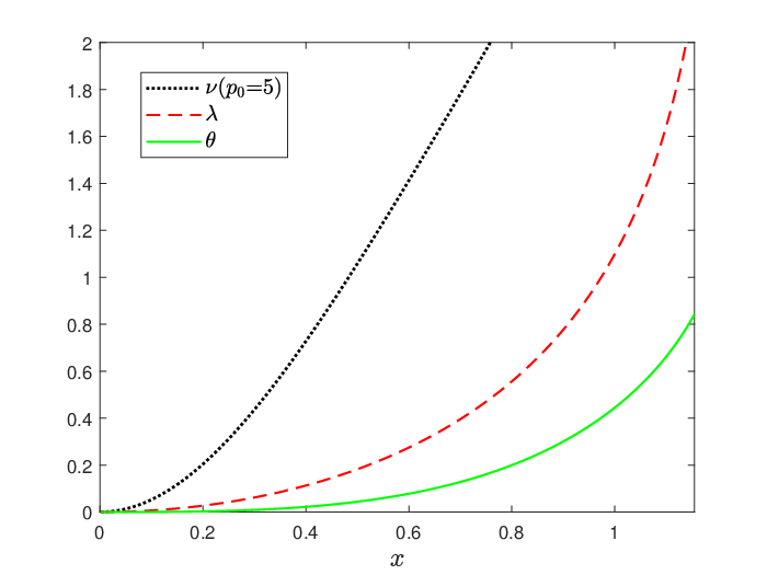
Refer to caption — Figure 1: Distributions of the metric functions $\lambda$ and $\nu$ at $p_{0}{=}5$ and the dimensionless charge $\theta$ inside a star within $0\leq x\leq\frac{2}{\sqrt{3}}$ .

The stellar boundary coordinate $x_{\mathrm{b}}$ is found from the condition $\phi(x_{\mathrm{b}})=1$ , which, according to (29), gives, with an accuracy of the order of $O(\Lambda_{\mathrm{q}})$ ,

x_{\mathrm{b}}=\frac{\sqrt{6\big(\phi_{0}{-1}\big)\big(2\phi_{0}{-}1\big)}}{3\phi_{0}{-}2}.

(32)

Obviously, $0\leq x_{\mathrm{b}}\leq\frac{2}{\sqrt{3}}$ . The quantities $x_{\mathrm{b}}$ and $\theta(x_{\mathrm{b}})$ are shown in Fig. 2 as a function of $\phi_{0}$ . The maximum values of $\theta(x_{\mathrm{b}})\approx 0.84$ and $x_{\mathrm{b}}\approx 1.15$ are reached when $\phi_{0}\rightarrow\infty$ .

Let us now turn to the equilibrium equations for the matter components. Equation (24) for $\Pi(x)$ can be integrated explicitly:

\Pi(x)=\ln\Bigg[\frac{3\phi_{0}{-}(3\phi_{0}{-}2)\sqrt{1{-}\frac{2x^{2}}{3}}}{2\sqrt{1{-}\frac{2x^{2}}{3}}}\Bigg].

(33)

Let us write Eq. (23) for the neutron chemical potential (given that $\tilde{q}_{\mathrm{n}}=0$ ):

\psi_{\mathrm{n}}(x)=e^{\lambda(x)/2{-}\Pi(x)}\psi_{\mathrm{n}}(0)=\frac{2\psi_{\mathrm{n}}(0)}{3\phi_{0}{-}(3\phi_{0}{-}2)\sqrt{1{-}\frac{2x^{2}}{3}}}.

(34)

Let us now consider $\phi(x)$ :

\phi(x)=\sum_{i}\psi_{i}Y_{i}\approx\psi_{\mathrm{n}}Y_{\mathrm{n}}+(\psi_{\mathrm{p}}{+}\psi_{\mathrm{e}})Y_{\mathrm{p}}=\psi_{\mathrm{n}}(x),

(35)

where we first used the LEN condition (approximate, with an accuracy of the order of $O(\Lambda_{\mathrm{q}})$ ) and then the beta-equilibrium condition. Expression (34) for $\psi_{\mathrm{n}}$ can then be rewritten with the same accuracy as

\psi_{\mathrm{n}}(x)=\frac{2\phi_{0}}{3\phi_{0}{-}(3\phi_{0}{-}2)\sqrt{1{-}\frac{2x^{2}}{3}}}.

(36)

This expression is identically satisfied at $x=0$ (given (35)), while at $x=x_{\mathrm{b}}$ defined by equality (32) it leads to the limit $\psi_{\mathrm{n}}(x_{\mathrm{b}})=1$ , as it must be.

Let us now turn to the case of charged particles. We need to calculate the integral of the polarization field in (23). It is

I_{\mathrm{E}}(x)\equiv\int\limits_{0}^{x}\frac{\theta(x^{\prime})}{x^{\prime 2}}e^{\Pi(x^{\prime})}dx^{\prime}=\frac{3}{8}\left[\Big(3\phi_{0}-2-3\phi_{0}\sqrt{1{-}\frac{2x^{2}}{3}}\Big)\frac{1}{x}\sqrt{\frac{3}{2}}\arcsin{\sqrt{\frac{2}{3}}x}-\right.\\ \left.{-}3\phi_{0}+4+(3\phi_{0}{-}2)\sqrt{1{-}\frac{2x^{2}}{3}}\right].

(37)

The chemical potentials of the charged matter components are then

\psi_{\mathrm{p,e}}(x)=\frac{\psi_{\mathrm{p,e}}(0)\pm\alpha_{\mathrm{e}}I_{\mathrm{E}}(x)}{\frac{3}{2}\phi_{0}{-}\big(\frac{3}{2}\phi_{0}{-}1\big)\sqrt{1{-}\frac{2x^{2}}{3}}},

(38)

where the upper and lower signs refer to the protons and electrons, respectively. So far the parameter $\alpha_{\mathrm{e}}$ has remained undetermined. Using (38) and the boundary condition for electrons $\psi_{\mathrm{e}}(x_{\mathrm{b}})=0$ , we will obtain

\alpha_{\mathrm{e}}=\frac{\psi_{\mathrm{e}}(0)}{I_{\mathrm{E}}(x_{\mathrm{b}})}.

(39)

The integral $I_{\mathrm{E}}(x_{\mathrm{b}})$ here is a function of $\phi_{0}\approx\psi_{\mathrm{n}}(0)\equiv\psi_{\mathrm{n0}}$ :

I_{\mathrm{E}}(x_{\mathrm{b}})=\frac{3}{8}\left[\frac{3\phi_{0}^{2}{-}6\phi_{0}{+}2}{\sqrt{(\phi_{0}{-}1)(2\phi_{0}{-}1)}}\arcsin\!\!\Big(\frac{2\sqrt{(\phi_{0}{-}1)(2\phi_{0}{-}1)}}{3\phi_{0}{-}2}\Big){-}2(\phi_{0}{-}2)\right].

(40)

Its behavior is presented Fig. 3, where the following asymptotics are also shown:

I_{\mathrm{E}}(x_{\mathrm{b}})=\begin{cases}\phi_{0}{-}1,&\phi_{0}\rightarrow 1,\\ \frac{3}{4}\left[\frac{3}{2\sqrt{2}}\arcsin\Big(\frac{2\sqrt{2}}{3}\Big){-}1\right]\phi_{0}\approx 0.23\phi_{0},&\phi_{0}\rightarrow\infty.\end{cases}

(41)

In the non-relativistic limit, $\phi_{0}{-}1=\psi_{\mathrm{n0}}{-}1$ is nothing but the neutron Fermi energy $E_{\mathrm{Fe}}^{\mathrm{n}}(0)$ , which, in view of the beta-equilibrium conditions, is $E_{\mathrm{Fe}}^{\mathrm{n}}=E_{\mathrm{Fe}}^{\mathrm{p}}+E_{\mathrm{Fe}}^{\mathrm{e}}$ . Given also that $\psi_{\mathrm{e0}}=E_{\mathrm{Fe}}^{\mathrm{e}}(0)$ for electrons, we will obtain Eq. (39) in the non-relativistic case in the form

\alpha_{\mathrm{e}}=\frac{E_{\mathrm{Fe}}^{\mathrm{e}}(0)}{E_{\mathrm{Fe}}^{\mathrm{e}}(0){+}E_{\mathrm{Fe}}^{\mathrm{p}}(0)},

(42)

i.e., the old result for polytropes (see Eq. (II.22) in Krivoruchenko et al. 2018).

NUMERICAL EXAMPLES

To illustrate the results obtained, it is necessary to understand the meaning of the parameter $\alpha_{\mathrm{e}}$ . For this purpose, we will write the expression for the total stellar charge $Q$ within a sphere of radius $r$ as

Q(r)=4\pi r_{0}^{3}n_{\mathrm{b}}\mathbf{e}\frac{\alpha_{\mathrm{e}}}{\Lambda_{\mathrm{G}}}\theta(x).

(43)

The number of baryons within the same sphere is

N(r)=4\pi r_{0}^{3}n_{\mathrm{b}}\int e^{\lambda(x)/2}x^{2}dx=4\pi r_{0}^{3}n_{\mathrm{b}}\theta(x).

(44)

The uncompensated charge per baryon in the star is then given by the expression (see also Hund and Kiessling 2021a, 2021b)

\frac{Q(r)}{N(r)}=\mathbf{e}\frac{\alpha_{\mathrm{e}}}{\Lambda_{\mathrm{G}}}.

(45)

In particular, the total stellar charge per baryon is equal to the value of (45) at $x=x_{\mathrm{b}}$ .

At a characteristic number of baryons in a star $N_{\mathrm{b}}\sim 10^{57}$ , an elementary charge $\mathbf{e}\approx 1.6\times 10^{-19}$ C, and $\Lambda_{\mathrm{G}}\sim 10^{36}$ , we obtain a typical total stellar charge $Q_{\mathrm{s}}\sim 100\alpha_{\mathrm{e}}$ C (see also Krivoruchenko et al. 2018). Thus, the parameter $\alpha_{\mathrm{e}}\sim O(1)$ determines the total stellar charge. As can be seen from Eq. (39), it is related to the electron chemical potential at zero. In an ordinary NS under the assumption of LEN (and, as a consequence, its zero total charge), specifying one parameter (for example, the central density) uniquely determines all properties of the configuration, in particular, its mass. In our case, apart from the parameter $\phi_{0}\approx\psi_{\mathrm{n0}}$ , we need to specify $\psi_{\mathrm{e0}}$ ( $\psi_{\mathrm{p0}}$ is determined from the beta-equilibrium conditions), thereby specifying both the total mass of the star and its charge.

Several examples of the derived distributions of the chemical potentials of the neutron, proton, and electron components for various initial conditions are shown in Fig. 4. As $\alpha_{\mathrm{e}}$ decreases, the electron chemical potential also drops (see Eq. (39)), while $\psi_{\mathrm{p}}$ approaches $\psi_{\mathrm{n}}$ (we can compare Eqs. (36) and (38) and take into account the beta-equilibrium condition).

How great can the parameter $\alpha_{\mathrm{e}}$ and, hence, the stellar charge be? It turns out that $\alpha_{\mathrm{e}}$ much greater than unity leads to an incorrect solution, as demonstrated by Fig. 5. The upper panel in the figure shows the behavior of the proton chemical potential near $\psi_{\mathrm{p}}\sim 1$ for several values of $\alpha_{\mathrm{e}}$ and fixed $\phi_{0}=5$ . At $\alpha_{\mathrm{e}}=1$ the curve $\psi_{\mathrm{p}}(x)$ with a finite slope runs into unity at the boundary of the star. At $\alpha_{\mathrm{e}}=2$ the slope at the boundary is almost zero, while at $\alpha_{\mathrm{e}}=3$ the curve runs into unity from below, from the inadmissible (in our approximation) region $\psi_{\mathrm{p}}<1$ ! Thus, the solution for the proton chemical potential is incorrect here, and the proton component, in fact, ends at $x\approx 0.3$ . This effect has a direct analog in the theory of polytropes. The Edmen functions shown on the lower panel of Fig. 5 for several values of the polytropic index $n$ can also have several roots. For example, the Edmen function for $n=1$ is $\sin(\xi)/\xi$ and becomes zero not only at $\xi=\pi$ , but also at $\xi=2\pi$ etc. However, the solution lying at $\xi>\pi$ is already unrealistic. At $\alpha_{\mathrm{e}}\gtrsim 2$ , although the solution obtained formally satisfies the boundary condition, it is not admissible in our case as well. Thus, large values of $\alpha_{\mathrm{e}}$ and, hence, the total stellar charge are also inadmissible.

ELECTROSPHERE

Is it possible to obtain a globally electroneutral stellar configuration with a total charge $Q_{\mathrm{s}}=0$ in the approximation under consideration? Formula (45) seems to suggest that this is possible only at $\alpha_{\mathrm{e}}=0$ , i.e., in the case of strict local electroneutrality. However, this is not the case: everywhere above, we used the significant condition that the number densities of all matter components become zero at one point. If we relax this requirement, then it is quite possible to construct a configuration in which the number density of, for example, electrons inside the star is lower than that of protons, but the electron component itself extends slightly farther, forming the so-called electrosphere on the stellar surface (Krivoruchenko et al. 2018), thereby compensating for the accumulated positive stellar charge. Let us estimate the parameters of this electrosphere in our approximation.

The electrosphere exists in a thin subsurface layer of thickness $r_{\mathrm{e}}$ , with $r_{\mathrm{e}}\ll r_{\mathrm{b}}$ , where the latter is the radius of the boundary of the baryon component. Hence, Eq. (4) for the charge $Q$ in the electrosphere is easily integrated. The requirement of $Q_{\mathrm{s}}=0$ gives the thickness of the electrosphere (cf. Eq. (A.9) from Krivoruchenko et al. 2018):

\frac{r_{\mathrm{e}}}{r_{\mathrm{b}}}=\frac{Q_{\mathrm{b}}}{4\pi r_{\mathrm{b}}^{3}\mathbf{e}n_{\mathrm{e}}}=\frac{\alpha_{\mathrm{e}}}{\Lambda_{\mathrm{G}}}\,\frac{\theta(x_{\mathrm{b}})}{x_{\mathrm{b}}^{3}e^{\lambda_{\mathrm{b}}/2}}\Big(\frac{n_{\mathrm{b}}}{n_{\mathrm{e}}}\Big)\sim 10^{-36},

(46)

where $Q_{\mathrm{b}}$ is the (positive) stellar charge at the boundary of the baryon component. According to the equilibrium equation (14), the electron chemical potential inside this electrosphere is zero with an accuracy of the order of $O(\Lambda_{\mathrm{G}}^{-1})$ .

CONCLUSIONS

We considered the structure of a locally non-electroneutral self-gravitating incompressible three-component fluid in general relativity. As in the case of Newtonian gravity, with regard to thermodynamic quantities like the pressure $P$ , the thermodynamic potential $\Phi$ , etc. (see Eqs. (21), (22) and (27)), the solution is a series in the small parameter $1/\Lambda_{\mathrm{G}}\sim 10^{-36}$ , where the first approximation is the classical electroneutral solution. The solution is degenerate, because it has no irregular component, in complete agreement with the analogous case in Newtonian gravity (see the Appendix from Krivoruchenko et al. (2018)). We found that the nonelectroneutrality may be neglected when calculating such macroscopic NS parameters as the mass and radius. Thus, we showed that the strange results of Belvedere et al. (2012) cannot be simply a consequence of LEN violation in general relativity. They are probably associated with their interpretation of the subtle effects occurring at the boundary of the stellar core. An electrosphere can appear here in our solution, but nothing like the sharp growth of the electric field found by these authors occurs there. The importance of a careful calculation of the phase boundaries when solving the problems of plasma polarization in astrophysical objects was pointed out by Iosilevskiy (see, e.g., Iosilevskiy 2009).

The main feature to which the deviation from LEN leads is contained in the equilibrium equations for the chemical potentials of the matter components (23). In them (for the charged components) the factor in front of the integral consists of two multipliers compensating for each other: one $\Lambda_{\mathrm{G}}$ is huge, while the other $(n_{\mathrm{p}}{-}n_{\mathrm{e}})/n_{\mathrm{b}}$ is small. This factor denoted by $\alpha_{\mathrm{e}}=O(1)$ enters into the final equilibrium equations for the individual matter components (38) and is responsible for the (already large) effect of deviation from LEN. In the long run, it also determines the total stellar charge (43). This nuance is a characteristic and very important feature of the problems of deviation from LEN in stars: despite the fact that this effect (and the polarization field generated by it) may be neglected with regard to large-scale parameters, when passing to the microlevel, it turns out that the force acting on a charged particle from this field is comparable to the gravitational force.

Despite the model nature of the problem considered, its solution seems an important step on the path of analyzing the structure of NSs with more realistic equations of state in the absence of strict LEN.

The work of N.I. Kramarev was supported by the ‘‘BAZIS’’ Foundation for the Development of Theoretical Physics and Mathematics (project no. 20-2-1-19-1).

We are also grateful to the anonymous referees whose remarks allowed our paper to be improved significantly.

REFERENCES

1. J. Bally, E. R. Harrison, Astrophys. J. 220, 743 (1978)

2. M.V. Beznogov and D.G. Yakovlev, Phys. Rev. Lett. 111, 161101 (2013)

3. G. Baym, C. Pethick, and P. Sutherland), Astrophys. J. 170, 299 (1971)

4. R. Belvedere, D. Pugliese, J. A. Rueda, R. Ruffini, S-Sh. Xue, Nuclear Physics A 883, 1–24 (2012)

5. Belvedere, R.; Rueda, Jorge A.; Ruffini, R., Astrophys. J. 799, 23 (2015)

6. S. Weinberg, Gravitation and Cosmology: Principles and Applications of the General Theory of Relativity (Wiley, New York, 1972).

7. A.B. Gorshkov and V.A. Baturin, Astronomy Reports 52, 760 (2008)

8. I.L. Iosilevskiy, J. Phys. A 42, 214008 (2009).

9. M.I. Krivoruchenko, D.K. Nadyozhin, and A.V. Yudin, Phys. Rev. D 97, 083016 (2018)

10. L. D. Landau and E. M. Lifshitz, Course of Theoretical Physics, Vol. 2: The Classical Theory of Fields (Pergamon, Oxford, 1975; Fizmatlit, Moscow, 2012).

11. R.E. O’Malley, ‘‘Singular Perturbation Methods for Ordinary Differential Equations’’, Springer-Verlag, New York (1991)

12. L. Neslusan, Astron. Astrophys. 372, 913 (2001)

13. E. Olson and M. Bailyn, Phys. Rev. D 12, 3030 (1975)

14. E. Olson and M. Bailyn, Phys. Rev. D 18, 2175 (1978)

15. J.M. Pearson, N. Chamel, A.Y. Potekhin, A.F. Fantina, C. Ducoin, A.K. Dutta, S. Goriely, MNRAS, 481, 3, 2994–3026 (2018)

16. S. Rosseland, Mon. Not. Roy. Astron. Soc. 84, 525 (1924)

17. M. Rotondo, Jorge A. Rueda, R. Ruffini, S.-S. Xue, Physics Letters B 701, 667-671 (2011)

18. J.L. Synge, Relativity: The General Theory, North-Holland, Amsterdam, (1960).

19. P. Haensel, A.Y. Potekhin, D.G. Yakovlev, ‘‘Neutron Stars 1: Equation of State and Structure’’, Springer, New York (2007)

20. P. Hund and M. K.-H. Kiessling, Phys. Rev. D, 103, 4 (2021)

21. P. Hund and M. K.-H. Kiessling, American J. of Phys., 89, 3, p.291-299 (2021)

22. E.L. Schatzman, ‘‘White Dwarfs’’, North-Holland, Amsterdam (1958)