A Linearized Boundary Control Method for the Acoustic Inverse Boundary Value Problem

Lauri Oksanen Thanks: lauri.oksanen@helsinki.fi Affiliation: Department of Mathematics and Statistics, University of Helsinki Tianyu Yang Thanks: yangti27@msu.edu Affiliation: Department of Computational Mathematics, Science and Engineering, Michigan State University Yang Yang Thanks: yangy5@msu.edu Affiliation: Department of Computational Mathematics, Science and Engineering, Michigan State University

Abstract

We develop a linearized boundary control method for the inverse boundary value problem of determining a potential in the acoustic wave equation from the Neumann-to-Dirichlet map. When the linearization is at the zero potential, we derive a reconstruction formula based on the boundary control method and prove that it is of Lipschitz-type stability. When the linearization is at a nonzero potential, we prove that the problem is of Hölder-type stability. The proposed reconstruction formula is implemented and evaluated using several numerical experiments to validate its feasibility.

1 Introduction

The paper is concerned with the linearized inverse boundary value problem (IBVP) for the acoustic wave equation with a potential. The goal is to derive stability estimates and reconstruction procedures to numerically compute a small perturbation of a known underlying potential, given the Neumann-to-Dirichlet map on the boundary of the domain.

Formulation. Specifically, let $T>0$ be a constant and $\Omega\subset\mathbb{R}^{n}$ be a bounded open subset with smooth boundary $\partial\Omega$ . Consider the following boundary value problem for the acoustic wave equation with potential:

\left\{\begin{array}[]{rcl}\Box_{c,q}u(t,x)&=&0,\quad\quad\quad\text{ in }(0,2T)\times\Omega\\ \partial_{\nu}u&=&f,\quad\quad\quad\text{ on }(0,2T)\times\partial\Omega\\ u(0,x)=\partial_{t}u(0,x)&=&0\quad\quad\quad\quad x\in\Omega.\end{array}\right.

(1)

Here $\Box_{c,q}$ is a linear wave operator defined as

\Box_{c,q}u(t,x):=\partial^{2}_{t}u(t,x)-c^{2}(x)\Delta u(t,x)+q(x)u(t,x);

$c(x)\in C^{\infty}(\overline{\Omega})$ is a smooth wave speed that is strictly positive, $q(x)\in L^{\infty}(\Omega)$ is a real-valued function. We denote this solution by $u^{f}(t,x)$ when it is necessary to specify the Neumann data.

Given $f\in C^{\infty}_{c}((0,2T)\times\partial\Omega)$ , the well-posedness of this problem is ensured by the standard theory for second order hyperbolic partial differential equations [20]. As a result, the following Neumann-to-Dirichlet (ND) map is well defined:

\Lambda_{c,q}f:=u^{f}|_{(0,2T)\times\partial\Omega}.

(2)

The inverse boundary value problem (IBVP) concerns recovery of the wave speed $c(x)$ and/or the potential $q(x)$ from knowledge of the ND map $\Lambda_{c,q}$ , that is to invert the nonlinear map $(c,q)\mapsto\Lambda_{c,q}$ .

Literature. The IBVP has been studied in the mathematical literature for a long time. The first coefficient determination result for a multidimensional wave equation, given the ND map, is by Rakesh and Symes [30]. They proved that a spatially varying potential is uniquely determined by the ND map in the case that $c=1$ . To our knowledge their method has never been implemented computationally.

For variable $c$ and $q=0$ , Belishev [3] proved that the leading order coefficient $c$ is uniquely determined using the boundary control (BC) method combined with Tataru’s unique continuation result [36]. The method has since been extended to many wave equations. We mention [7] for a generalization to Riemannian manifolds, and [23] for a result covering all symmetric time-independent lower order perturbations of the wave operator. Non-symmetric, time-dependent and matrix-valued lower order perturbations were recovered in [19] [24], and [25], respectively. For a review of the method, we refer to [5, 21].

The BC method has been implemented numerically to reconstruct the wave speed in [4], and subsequently in [6, 16, 29, 37]. The implementations [4, 6, 16] involve solving unstable control problems, whereas [29, 37] are based on solving stable control problems but with target functions exhibiting exponential growth or decay. The exponential behaviour leads to instability as well. On the other hand, the linearized approach introduced in the present paper is stable. It should be mentioned that the BC method can be implemented in a stable way in the one-dimensional case, see [22]. For an interesting application of a variant of the method in the one-dimensional case, see [11] on detection of blockage in networks.

Under suitable geometric assumptions, it can be proven that the problem to recover the speed of sound is Hölder stable [31, 32], even when the speed is given by an anisotropic Riemannian metric. Moreover, a low-pass version of $c$ can be recovered in a Lipschitz stable manner [26]. The problem to recover $q$ is Hölder stable assuming, again, that the geometry is nice enough [8, 27, 35]. To our knowledge, the method, based on using high frequency solutions to the wave equation and yielding the latter three results, has not been implemented computationally. Stability results applicable to general geometries have been proven using the BC method in [2], with an abstract modulus continuity, and very recently in [12, 13], with a doubly logarithmic modulus of continuity.

Finally, let us mention that recently there has been a lot of activity related to recovery of time-dependent coefficients in wave equations, see for example [33], [1], and the references therein for up-to-date results. The first result in the time-dependent context was obtained in [34].

Linearization. Throughout the paper, we will assume the wave speed $c=c_{0}(x)$ is known. Here $c_{0}(x)\in C^{\infty}(\overline{\Omega})$ is a smooth wave speed that is strictly positive. Then the IBVP only concerns recovery of the potential $q$ .

We will study the linearization of this problem by linearzing the map $q\mapsto\Lambda_{c_{0},q}$ . For this purpose, we write

q(x)=q_{0}(x)+\epsilon\dot{q}(x),\quad\quad u(t,x)=u_{0}(t,x)+\epsilon\dot{u}(t,x)

where $q_{0}$ is a known background potential and $u_{0}$ is the background solution. Insert these into (1). Equating the $O(1)$ -terms gives

\left\{\begin{array}[]{rcll}\Box_{c_{0},q_{0}}u_{0}(t,x)&=&0,&\quad\text{ in }(0,2T)\times\Omega\\ \partial_{\nu}u_{0}&=&f,&\quad\text{ on }(0,2T)\times\partial\Omega\\ u_{0}(0,x)=\partial_{t}u_{0}(0,x)&=&0,&\quad x\in\Omega.\end{array}\right.

(3)

Equating the $O(\epsilon)$ -terms gives

\left\{\begin{array}[]{rcll}\Box_{c_{0},q_{0}}\dot{u}(t,x)&=&u_{0}(t,x)\dot{q}(x),&\quad\text{ in }(0,2T)\times\Omega\\ \partial_{\nu}\dot{u}&=&0,&\quad\text{ on }(0,2T)\times\partial\Omega\\ \dot{u}(0,x)=\partial_{t}\dot{u}(0,x)&=&0&\quad x\in\Omega.\end{array}\right.

(4)

Write the ND map $\Lambda_{q}=\Lambda_{q_{0}}+\epsilon\dot{\Lambda}_{\dot{q}}$ , where $\Lambda_{q_{0}}$ is the ND map for the unperturbed boundary value problem (3), and $\dot{\Lambda}_{\dot{q}}$ is defined as

\dot{\Lambda}_{\dot{q}}:f\mapsto\dot{u}|_{(0,2T)\times\partial\Omega}.

(5)

Note that the unperturbed problem (3) can be explicitly solved to obtain $u_{0}$ and $\Lambda_{q_{0}}$ , since $c_{0}$ and $q_{0}$ are known. As before, we will write $\dot{u}=\dot{u}^{f}:=\dot{\Lambda}_{\dot{q}}f$ if it is necessary to specify the Neumann data $f$ . Then the linearized IBVP concerns recovery of the potential $\dot{q}$ from $\dot{\Lambda}_{\dot{q}}$ .

Main Results. The main contribution of this paper consists of several results regarding reconstruction of $\dot{q}$ based on the BC method. For constant $c_{0}$ and $q_{0}=0$ , we derive a reconstruction formula for $\dot{q}$ in Theorem 5, and prove that the reconstruction is of Lipschitz-type stability in Theorem 7. For constant $c_{0}$ and $q_{0}\neq 0$ , we derive a reconstruction formula in Theorem 8, and prove that the reconstruction is of Hölder-type stability in Theorem 9. The formula is implemented and validated using numerical experiments, showing reliable reconstructions.

Paper Structure. The paper is organized as follows. Section 2 reviews a few fundamental concepts and results in the boundary control theory. Section 3 consists of an integral identity and a controllability result that are essential to the development of our method. Section 4 establishes stability estimates and reconstruction formulae for the linearized IBVP, which are the central results of the paper. Section 5 is devoted to numerical implementation of the reconstruction formulae as well as numerical experiments to assess performance of the proposed reconstructions.

2 Preliminaries

Introduce some notations: Given a function $u(t,x)$ , we write $u(t)=u(t,\cdot)$ for the spatial part as a function of $x$ . Introduce the time reversal operator $R:L^{2}([0,T]\times\partial\Omega)\rightarrow L^{2}([0,T]\times\partial\Omega)$ ,

Ru(t,\cdot):=u(T-t,\cdot),\quad\quad 0<t<T;

(6)

and the low-pass filter $J:L^{2}([0,2T]\times\partial\Omega)\rightarrow L^{2}([0,T]\times\partial\Omega)$

Jf(t,\cdot):=\frac{1}{2}\int^{2T-t}_{t}f(\tau,\cdot)\,d\tau,\quad\quad 0<t<T.

(7)

We write $P_{T}:L^{2}((0,2T)\times\partial\Omega)\rightarrow L^{2}((0,T)\times\partial\Omega)$ for the orthogonal projection via restriction. Its adjoint operator $P^{\ast}_{T}:L^{2}((0,T)\times\partial\Omega)\rightarrow L^{2}((0,2T)\times\partial\Omega)$ is the extension by zero from $(0,T)$ to $(0,2T)$ . Let $\mathcal{T}_{D}$ and $\mathcal{T}_{N}$ be the Dirichlet and Neumann trace operators respectively, that is,

\mathcal{T}_{D}u(t,\cdot)=u(t,\cdot)|_{\partial\Omega},\quad\quad\quad\mathcal{T}_{N}u(t,\cdot)=\partial_{\nu}u(t,\cdot)|_{\partial\Omega}.

Introduce the connecting operator

K:=J\Lambda_{q}P^{\ast}_{T}-R\Lambda_{q,T}RJP^{\ast}_{T}

(8)

where $\Lambda_{q,T}f:=P_{T}(\Lambda_{q}f)$ . Then the following Blagoves̆c̆enskiĭ’s identity holds [9, 10, 15, 28].

Proposition 1.

Let $u^{f},u^{h}$ be the solutions of (1) with Neumann traces $f,h\in L^{2}((0,T)\times\partial\Omega)$ , respectively. Then

(u^{f}(T),u^{h}(T))_{L^{2}(\Omega,c_{0}^{-2}dx)}=(f,Kh)_{L^{2}((0,T)\times\partial\Omega)}=(Kf,h)_{L^{2}((0,T)\times\partial\Omega)}.

(9)

Proof.

We first prove this for $f,h\in C^{\infty}_{c}((0,T)\times\partial\Omega)$ . Define

I(t,s):=(u^{f}(t),u^{h}(s))_{L^{2}(\Omega,c_{0}^{-2}dx)}.

We compute

	$\displaystyle(\partial^{2}_{t}-\partial^{2}_{s})I(t,s)$
$\displaystyle=$	$\displaystyle((\Delta+qc_{0}^{-2})u^{f}(t),u^{h}(s))_{L^{2}(\Omega)}-(u^{f}(t),(\Delta+qc_{0}^{-2})u^{h}(s))_{L^{2}(\Omega)}$
$\displaystyle=$	$\displaystyle(f(t),\Lambda_{q}P^{}_{T}h(s))_{L^{2}(\partial\Omega)}-(\Lambda_{q}P^{}_{T}f(t),h(s))_{L^{2}(\partial\Omega)},$	(10)

where the last equality follows from integration by parts. On the other hand, $I(0,s)=\partial_{t}I(0,s)=0$ since $u^{f}(0,x)=\partial_{t}u^{f}(0,x)=0$ . Solve the inhomogeneous $1$ D wave equation (10) together with these initial conditions to obtain

	$\displaystyle I(T,T)$	$\displaystyle=\frac{1}{2}\int^{T}_{0}\int^{2T-t}_{t}\left[(f(t),\Lambda_{q}P^{}_{T}h(\sigma))_{L^{2}(\partial\Omega)}-(\Lambda_{q}P^{}_{T}f(t),h(\sigma))_{L^{2}(\partial\Omega)}\right]\,d\sigma dt\vskip 4.30554pt$
		$\displaystyle=\int^{T}_{0}[(f(t),\frac{1}{2}\int^{2T-t}_{t}\Lambda_{q}P^{}_{T}h(\sigma)\,d\sigma)_{L^{2}(\partial\Omega)}-(\Lambda_{q}P^{}_{T}f(t),\frac{1}{2}\int^{2T-t}_{t}h(\sigma)\,d\sigma)_{L^{2}(\partial\Omega)}]\,dt\vskip 4.30554pt$
		$\displaystyle=(f,J\Lambda_{q}P^{}_{T}h)_{L^{2}((0,T)\times\partial\Omega)}-(P_{T}(\Lambda_{q}f),JP^{}_{T}h)_{L^{2}((0,T)\times\partial\Omega)}.$

Using the relations $P_{T}(\Lambda_{q}f)=\Lambda_{q,T}f$ and $\Lambda^{\ast}_{q,T}=R\Lambda_{q,T}R$ in $L^{2}((0,T)\times\partial\Omega)$ , we have

	$\displaystyle I(T,T)$	$\displaystyle=(f,J\Lambda_{q}P^{\ast}_{T}h)_{L^{2}((0,T)\times\partial\Omega)}-(\Lambda_{q,T}f,JP^{\ast}_{T}h)_{L^{2}((0,T)\times\partial\Omega)}$
		$\displaystyle=(f,J\Lambda_{q}P^{\ast}_{T}h)_{L^{2}((0,T)\times\partial\Omega)}-(f,R\Lambda_{q,T}RJP^{\ast}_{T}h)_{L^{2}((0,T)\times\partial\Omega)}$
		$\displaystyle=(f,Kh)_{L^{2}((0,T)\times\partial\Omega)}$

For general $f,h\in L^{2}((0,T)\times\partial\Omega)$ , simply notice that $K$ is a continuous operator and that compactly supported smooth functions are dense in $L^{2}$ . The proof is completed. ∎

Corollary 2.

Suppose $f,h\in C^{\infty}_{c}((0,T]\times\partial\Omega)$ . Then

(c_{0}^{2}\Delta u^{f}(T)-qu^{f}(T),u^{h}(T))_{L^{2}(\Omega,c_{0}^{-2}dx)}=(\partial^{2}_{t}f,Kh)_{L^{2}((0,T)\times\partial\Omega)}=(K\partial^{2}_{t}f,h)_{L^{2}((0,T)\times\partial\Omega)}.

(11)

Proof.

Replacing $f$ by $\partial^{2}_{t}f$ in (9), we get

(u^{\partial^{2}_{t}f}(T),u^{h}(T))_{L^{2}(\Omega,c_{0}^{-2}dx)}=(\partial^{2}_{t}f,Kh)_{L^{2}((0,T)\times\partial\Omega)}=(K\partial^{2}_{t}f,h)_{L^{2}((0,T)\times\partial\Omega)}.

As both $u^{\partial^{2}_{t}f}$ and $\partial^{2}_{t}u^{f}$ satisfy (1) with $f$ replaced by $\partial^{2}_{t}f$ , they must be equal thanks to the well-posedness of the boundary value problem. We conclude

u^{\partial^{2}_{t}f}=\partial^{2}_{t}u^{f}=c_{0}^{2}\Delta u^{f}-qu^{f}.

∎

Recall that we write $\Lambda_{q}=\Lambda_{q_{0}}+\epsilon\dot{\Lambda}_{\dot{q}}$ in the linearization setting. Accordingly, we write $K=K_{0}+\epsilon\dot{K}$ . Here $K_{0}$ is the connecting operator for the background medium:

K_{0}:=J\Lambda_{q_{0}}P^{\ast}_{T}-R\Lambda_{q_{0},T}RJP^{\ast}_{T}.

(12)

$K_{0}$ can be explicitly computed since $\Lambda_{c,q_{0}}$ is known. $\dot{K}$ is the resulting perturbation in the connecting operator:

\dot{K}:=J\dot{\Lambda}_{\dot{q}}P^{\ast}_{T}-R\dot{\Lambda}_{\dot{q},T}RJP^{\ast}_{T}.

(13)

$\dot{K}$ can be explicitly computed once $\dot{\Lambda}_{\dot{q}}$ is given.

3 Integral Identity and Controllability

First, we derive an integral identity that is essential to the development of the reconstruction procedure. We write $\dot{\Lambda}$ for $\dot{\Lambda}_{\dot{q}}$ when there is no risk of confusion.

Proposition 3.

Let $\lambda\in\mathbb{R}$ be a real number. If $f,h\in C^{\infty}_{c}((0,T]\times\partial\Omega)$ satisfy

[\Delta-q_{0}c_{0}^{-2}+\lambda c_{0}^{-2}]u_{0}^{f}(T)=[\Delta-q_{0}c_{0}^{-2}+\lambda c_{0}^{-2}]u_{0}^{h}(T)=0\quad\text{ in }\Omega,

(14)

then the following identity holds:

-(\dot{q}c_{0}^{-2}u_{0}^{f}(T),u^{h}_{0}(T))_{L^{2}(\Omega)}=(\partial^{2}_{t}f+\lambda f,\dot{K}h)_{L^{2}((0,T)\times\partial\Omega)}+(\dot{\Lambda}f(T),h(T))_{L^{2}(\partial\Omega)}

(15)

Proof.

For $f,h\in C^{\infty}_{c}((0,T)\times\partial\Omega)$ , we will make use of (9) (11) to obtain some identities. First, let $\epsilon=0$ in (9) we obtain

(u_{0}^{f}(T),u_{0}^{h}(T))_{L^{2}(\Omega,c_{0}^{-2}dx)}=(f,K_{0}h)_{L^{2}((0,T)\times\partial\Omega)}=(K_{0}f,h)_{L^{2}((0,T)\times\partial\Omega)}.

Next, differentiating (9) in $\epsilon$ and let $\epsilon=0$ , we obtain

		$\displaystyle(f,\dot{K}h)_{L^{2}((0,T)\times\partial\Omega)}=(\dot{K}f,h)_{L^{2}((0,T)\times\partial\Omega)}$
	$\displaystyle=$	$\displaystyle(\dot{u}^{f}(T),u_{0}^{h}(T))_{L^{2}(\Omega,c_{0}^{-2}dx)}+(u_{0}^{f}(T),\dot{u}^{h}(T))_{L^{2}(\Omega,c_{0}^{-2}dx)}.$		(16)

Similarly, let $\epsilon=0$ in (11) we obtain

(c_{0}^{2}\Delta u_{0}^{f}(T)-qu_{0}^{f}(T),u_{0}^{h}(T))_{L^{2}(\Omega,c_{0}^{-2}dx)}=(\partial^{2}_{t}f,K_{0}h)_{L^{2}((0,T)\times\partial\Omega)}=(K_{0}\partial^{2}_{t}f,h)_{L^{2}((0,T)\times\partial\Omega)}.

Next, differentiating (11) in $\epsilon$ and let $\epsilon=0$ , we obtain

	$\displaystyle(\partial^{2}_{t}f,\dot{K}h)_{L^{2}((0,T)\times\partial\Omega)}=(\dot{K}\partial^{2}_{t}f,h)_{L^{2}((0,T)\times\partial\Omega)}$
$\displaystyle=$	$\displaystyle(c_{0}^{2}\Delta\dot{u}^{f}(T)-\dot{q}u_{0}^{f}(T)-q_{0}\dot{u}^{f}(T),u_{0}^{h}(T))_{L^{2}(\Omega,c_{0}^{-2}dx)}$
$\displaystyle+$	$\displaystyle(c_{0}^{2}\Delta u_{0}^{f}(T)-q_{0}u_{0}^{f}(T),\dot{u}^{h}(T))_{L^{2}(\Omega,c_{0}^{-2}dx)}$
$\displaystyle=$	$\displaystyle\underbrace{(\Delta\dot{u}^{f}(T),u_{0}^{h}(T))_{L^{2}(\Omega)}-(q_{0}c_{0}^{-2}\dot{u}^{f}(T),u_{0}^{h}(T))_{L^{2}(\Omega)}}_{:=I_{1}}$
$\displaystyle-$	$\displaystyle(\dot{q}c_{0}^{-2}u_{0}^{f}(T),u_{0}^{h}(T))_{L^{2}(\Omega)}$
$\displaystyle+$	$\displaystyle\underbrace{(\Delta u_{0}^{f}(T),\dot{u}^{h}(T))_{L^{2}(\Omega)}-(q_{0}c_{0}^{-2}u_{0}^{f}(T),\dot{u}^{h}(T))_{L^{2}(\Omega)}}_{:=I_{2}}$	(17)

where $L^{2}(\Omega)=L^{2}(\Omega,dx)$ is the $L^{2}$ -space equipped with the usual Lebesgue measure.

For $I_{1}$ , we integrate the first term by parts and use the fact that $\partial_{\nu}\dot{u}=0$ and $\dot{u}^{f}|_{(0,2T)\times\partial\Omega}=\dot{\Lambda}f$ to get

	$\displaystyle I_{1}=$	$\displaystyle(\Delta\dot{u}^{f}(T),u_{0}^{h}(T))_{L^{2}(\Omega)}-(q_{0}c_{0}^{-2}\dot{u}^{f}(T),u_{0}^{h}(T))_{L^{2}(\Omega)}$
	$\displaystyle=$	$\displaystyle(\dot{u}^{f}(T),\Delta u_{0}^{h}(T))_{L^{2}(\Omega)}-(\dot{\Lambda}f(T),\partial_{\nu}u_{0}^{h}(T))_{L^{2}(\partial\Omega)}-(q_{0}c_{0}^{-2}\dot{u}^{f}(T),u_{0}^{h}(T))_{L^{2}(\Omega)}$
	$\displaystyle=$	$\displaystyle(\dot{u}^{f}(T),[\Delta-q_{0}c_{0}^{-2}]u_{0}^{h}(T))_{L^{2}(\Omega)}-(\dot{\Lambda}f(T),h(T))_{L^{2}(\partial\Omega)}.$

On the other hand, combing the terms in $I_{2}$ we have

I_{2}=([\Delta-q_{0}c_{0}^{-2}]u_{0}^{f}(T),\dot{u}^{h}(T))_{L^{2}(\Omega)}.

Insert these expressions for $I_{1}$ and $I_{2}$ into (17), then add (16) multiplied by $\lambda\in\mathbb{R}$ to get

		$\displaystyle(\partial^{2}_{t}f+\lambda f,\dot{K}h)_{L^{2}((0,T)\times\partial\Omega)}+(\dot{\Lambda}f(T),h(T))_{L^{2}(\partial\Omega)}$
	$\displaystyle=$	$\displaystyle(\dot{u}^{f}(T),[\Delta-q_{0}c_{0}^{-2}+\lambda c_{0}^{-2}]u_{0}^{h}(T))_{L^{2}(\Omega)}-(\dot{q}c_{0}^{-2}u_{0}^{f}(T),u_{0}^{h}(T))_{L^{2}(\Omega)}+([\Delta-q_{0}c_{0}^{-2}+\lambda c_{0}^{-2}]u_{0}^{f}(T),\dot{u}^{h}(T))_{L^{2}(\Omega)}.$		(18)

If $[\Delta-q_{0}c_{0}^{-2}+\lambda c_{0}^{-2}]u_{0}^{f}(T)=[\Delta-q_{0}c_{0}^{-2}+\lambda c_{0}^{-2}]u_{0}^{h}(T)=0\text{ in }\Omega$ , the first term and last term on the right-hand side vanish, resulting in (15). ∎

Next, we establish a boundary control estimate. Given a strictly positive $c_{0}\in C^{\infty}(\overline{\Omega})$ , we will write $g:=c_{0}^{-2}dx^{2}$ for the Riemannian metric associated to $c_{0}$ , and denote by $S\overline{\Omega}$ the unit sphere bundle over the closure $\overline{\Omega}$ of $\Omega$ .

Proposition 4.

Let $c_{0}\in C^{\infty}(\overline{\Omega})$ be strictly positive and $q_{0}\in C^{\infty}(\overline{\Omega})$ . Suppose that all maximal¹¹ 1 For a maximal geodesic $\gamma:[a,b]\to\overline{\Omega}$ there may exists $t\in(a,b)$ such that $\gamma(t)\in\partial\Omega$ . The geodesics are maximal on the closed set $\overline{\Omega}$ . geodesics on $(\overline{\Omega},g)$ have length strictly less than some fixed $T>0$ . Then for any $\phi\in C^{\infty}(\overline{\Omega})$ there is $f\in C_{c}^{\infty}((0,T]\times\partial\Omega)$ such that

u_{0}^{f}(T)=\phi\quad\text{in $\Omega$},

(19)

where $u_{0}$ is the solution of (3). Moreover, there is $C>0$ , independent of $\phi$ , such that

\lVert f\rVert_{H^{2}((0,T)\times\partial\Omega)}\leq C\lVert\phi\rVert_{H^{4}(\Omega)}.

(20)

Proof.

There is small $\delta>0$ such that the maximal geodesics have length less than $T^{*}:=T-2\delta$ . We extend $c_{0}$ and $q_{0}$ smoothly to $\mathbb{R}^{n}$ . Then there is a compact domain $\mathcal{K}$ with smooth boundary such that $\overline{\Omega}$ is contained in the interior of $\mathcal{K}$ and that the extended tensor $g=c_{0}^{-2}dx$ gives a Riemannian metric on $\mathcal{K}$ . Let $x\in\overline{\Omega}$ and let $\xi\in S_{x}\overline{\Omega}$ , that is, $\xi$ is a unit vector with respect to $g$ at $x$ . Write $\gamma_{x,\xi}:[a,b]\to\overline{\Omega}$ for the maximal geodesic with the initial data $(x,\xi)$ . Then $b<T^{*}$ . We extend $\gamma_{x,\xi}$ as the maximal geodesic in $\mathcal{K}$ and write $\gamma_{x,\xi}:[\hat{a},\hat{b}]\to\mathcal{K}$ . Then there are $t_{j}>b$ such that $t_{j}\to b$ and $\gamma_{x,\xi}(t_{j})\notin\overline{\Omega}$ . If $\hat{b}<T^{*}$ we extend $\gamma_{x,\xi}$ to $[\hat{a},T^{*}]$ by setting $\gamma_{x,\xi}(t)=\gamma_{x,\xi}(\hat{b})$ for $t>\hat{b}$ . Then the function

\displaystyle\rho(x,\xi):=\max\{d(\gamma_{x,\xi}(t),\overline{\Omega}):t\in[0,T^{*}]\}

satisfies $\rho(x,\xi)>0$ . Let us show that $\rho$ is continuous. It follows from the smoothness of the geodesic flow and the triangle inequality that the function

\displaystyle S\overline{\Omega}\times[0,T^{*}]\times\overline{\Omega}\ni(x,\xi,t,y)\mapsto d(\gamma_{x,\xi}(t),y)

is uniformly continuous. By Lemma 10 in the appendix, the function

\displaystyle S\overline{\Omega}\times[0,T^{*}]\ni(x,\xi,t)\mapsto d(\gamma_{x,\xi}(t),\overline{\Omega}),

is uniformly continuous, and so is $\rho$ .

We have show that the continuous function $\rho$ is strictly positive on the compact set $S\overline{\Omega}$ . Thus there is an open set $\omega_{0}$ such that $\overline{\omega_{0}}\subset\mathcal{K}\setminus\overline{\Omega}$ and that all geodesics $\gamma_{x,\xi}$ with $(x,\xi)\in S\overline{\Omega}$ intersect $\omega_{0}$ in time $T^{*}$ .

We choose $\eta\in C_{c}^{\infty}(0,T)$ taking values in $[0,1]$ and satisfying $\eta=1$ on $[\delta,T-\delta]$ , and $\chi\in C^{\infty}_{c}(\mathcal{K}\setminus\overline{\Omega})$ satisfying $\chi=1$ on $\omega_{0}$ . Finally, we choose an extension $\phi\in C_{c}^{\infty}(\mathcal{K})$ . Now [18, Theorem 5.1] implies that there is $Y\in C^{\infty}((0,T)\times(\mathcal{K}\setminus\overline{\Omega}))$ such that

\displaystyle\begin{cases}\Box_{c_{0},q_{0}}v=\eta\chi Y,\\ v|_{x\in\partial\mathcal{K}}=0,\\ v|_{t=T}=\phi,\ \partial_{t}v|_{t=T}=0,\\ v|_{t=0}=0,\ \partial_{t}v|_{t=0}=0.\end{cases}

(21)

We extend $v$ to $(0,2T)\times\mathcal{K}$ by solving

\displaystyle\begin{cases}\Box_{c_{0},q_{0}}v=0,\\ v|_{x\in\partial\mathcal{K}}=0,\\ v|_{t=T}=\phi,\ \partial_{t}v|_{t=T}=0,\end{cases}

and set $f=\partial_{\nu}v|_{x\in\partial\Omega}$ . As $\eta(t)=0$ when $t$ is close to zero and as $v$ satisfies vanishing initial conditions at $t=0$ , also $f(t,x)=0$ for $t$ near zero.

It remains to show estimate (20). The extension of $\phi$ can be chosen so that

\displaystyle\lVert\phi\rVert_{H^{4}(\mathcal{K})}\leq C\lVert\phi\rVert_{H^{4}(\Omega)}.

By [18, Theorem 5.1] there is a map

\displaystyle G:H^{4}(\mathcal{K})\to H^{3}(\mathcal{K})\times H^{2}(\mathcal{K}),\quad G(\phi)=(Y|_{t=0},\partial_{t}Y|_{t=0}),

(22)

and $Y$ satisfies

\displaystyle\begin{cases}\Box_{c_{0},q_{0}}Y=0,\\ Y|_{x\in\partial\mathcal{K}}=0.\end{cases}

As continuity of (22) is not explicitly stated in [18], we will show the continuity for the convenience of the reader.

Due to the closed graph theorem it is enough to show that if $\phi_{j}\to\phi$ in $H^{4}(\mathcal{K})$ and $G(\phi_{j})\to(Y_{0},Y_{1})$ in $H^{3}(\mathcal{K})\times H^{2}(\mathcal{K})$ then $G(\phi)=(Y_{0},Y_{1})$ . We define $v_{j}$ and $Y_{j}$ by

\displaystyle\begin{cases}\Box_{c_{0},q_{0}}v_{j}=\eta\chi Y_{j},\\ v_{j}|_{x\in\partial\mathcal{K}}=0,\\ v_{j}|_{t=0}=0,\ \partial_{t}v_{j}|_{t=0}=0,\end{cases}\qquad\begin{cases}\Box_{c_{0},q_{0}}Y_{j}=0,\\ Y_{j}|_{x\in\partial\mathcal{K}}=0,\\ (Y_{j}|_{t=0},\partial_{t}Y_{j}|_{t=0})=F(\phi_{j}),\end{cases}

Then $v_{j}\to v$ and $Y_{j}\to Y$ where $v$ and $Y$ solve

\displaystyle\begin{cases}\Box_{c_{0},q_{0}}v=\eta\chi Y,\\ v|_{x\in\partial\mathcal{K}}=0,\\ v|_{t=0}=0,\ \partial_{t}v|_{t=0}=0,\end{cases}\qquad\begin{cases}\Box_{c_{0},q_{0}}Y=0,\\ Y|_{x\in\partial\mathcal{K}}=0,\\ (Y|_{t=0},\partial_{t}Y|_{t=0})=(Y_{0},Y_{1}),\end{cases}

and also

\displaystyle v_{j}|_{t=T}=\lim_{j}v_{j}|_{t=T}=\lim_{j}\phi_{j}=\phi,\quad\partial_{t}v|_{t=T}=\lim_{j}\partial_{t}v_{j}|_{t=T}=0.

But the control given by [18, Theorem 5.1] for $\phi$ is characterized by the following system

\displaystyle\begin{cases}\Box_{c_{0},q_{0}}v=\eta\chi Y,\\ v|_{x\in\partial\mathcal{K}}=0,\\ v|_{t=0}=\phi,\ \partial_{t}u|_{t=0}=0,\\ v|_{t=T}=0,\ \partial_{t}u|_{t=T}=0,\end{cases}\qquad\begin{cases}\Box_{c_{0},q_{0}}Y=0,\\ Y|_{x\in\partial\mathcal{K}}=0,\end{cases}

see [14]. Hence the control $Y$ that we obtained as the limit coincides with that given by [18, Theorem 5.1], and $G(\phi)=(Y_{0},Y_{1})$ .

By [18, Theorem 5.1] the initial data $G(\phi)$ satisfies suitable compatibility conditions so that $Y\in H^{3}((0,T)\times\mathcal{K})$ . Moreover, solving (21) from the initial data at $t=0$ , while discarding the constaint at $t=T$ , gives

\displaystyle\lVert v\rVert_{H^{4}((0,T)\times\mathcal{K})}\leq C\lVert Y\rVert_{H^{3}((0,T)\times\mathcal{K})}\leq C\lVert G(\phi)\rVert_{H^{3}(\mathcal{K})\times H^{2}(\mathcal{K})}\leq C\lVert\phi\rVert_{H^{4}(\mathcal{K})}.

∎

Remark: Solvability of an equation like (19) is a central question in the boundary control theory. There are other results which ensure the solvability in other function spaces. For example, if we define

W_{0}:L^{2}((0,T)\times\partial\Omega)\rightarrow L^{2}(\Omega,c_{0}^{-2}dx),\quad\quad\quad W_{0}f=u^{f}(T).

This clearly is a bounded linear operator. Moreover, if $T>0$ is large enough, the range $Ran(W_{0})$ is dense in $L^{2}(\Omega)$ by Tataru’s unique continuation [36]. If we further assume that the continuous observability condition [26] holds for the background wave solution, then $W_{0}$ is surjective, that is, $Ran(W_{0})=L^{2}(\Omega)$ . This ensures the existence of solutions $f,h\in L^{2}((0,T)\times\partial\Omega)$ for the equation (23). However, such $L^{2}$ -regularity is insufficient for our purpose, as we need $\partial^{2}_{t}f$ to exist, see (24).

4 Stability and Reconstruction

We will make use of Proposition 3 and Proposition 4 to derive stability estimate and reconstruction formulae for $\dot{q}$ , on the premise that the wave speed is constant. Without loss of generality, we take $c_{0}=1$ . The discussion is separate for vanishing and non-vanishing background potentials $q_{0}$ .

4.1 Case 1: $c_{0}=1$ and $q_{0}=0$

We take $\lambda\geq 0$ and dimension $n\geq 1$ , then the equation (14) for $u^{f}_{0}(T)$ and $u^{h}_{0}(T)$ becomes the Helmholtz equation

(\Delta+\lambda)u_{0}^{f}(T)=(\Delta+\lambda)u_{0}^{h}(T)=0\quad\text{ in }\Omega.

A class of Helmholtz solutions are the plane waves $e^{i\sqrt{\lambda}\theta\cdot x}$ where $\theta\in\mathbb{S}^{n-1}$ is an arbitrary unit vector. Moreover, Proposition 4 ensures the existence of $f,h\in C^{\infty}_{c}((0,T]\times\partial\Omega)$ such that

u^{f}_{0}(T)=u^{h}_{0}(T)=e^{i\sqrt{\lambda}\theta\cdot x}.

(23)

Theorem 5.

Suppose $c_{0}=1$ and $q_{0}=0$ . Then the Fourier transform $\hat{\dot{q}}$ of $\dot{q}$ can be reconstructed as follows:

\hat{\dot{q}}(2\sqrt{\lambda}\theta)=-(\partial^{2}_{t}f+\lambda f,\dot{K}h)_{L^{2}((0,T)\times\partial\Omega)}-(\dot{\Lambda}f(T),h(T))_{L^{2}(\partial\Omega)}

(24)

where $f,h\in C^{\infty}_{c}((0,T]\times\partial\Omega)$ are solutions to (23).

Proof.

The formula is obtained by inserting $u^{f}_{0}(T)=u^{h}_{0}(T)=e^{i\sqrt{\lambda}\theta\cdot x}$ into (15). As $\lambda\geq 0$ and $\theta$ are arbitrary, it recovers the Fourier transform of $\dot{q}$ everywhere. ∎

Remark 6.

An explicit procedure to solve for $f$ and $h$ from (23) is explained in Section 5.1.

Next, we show that the reconstruction above has Lipschitz-type stability. As the inverse problem is linear, it suffices to bound $\dot{q}$ using continuous functions of $\dot{\Lambda}$ .

Theorem 7.

Suppose $c_{0}=1$ and $q_{0}=0$ . There exists a constant $C>0$ , independent of $\lambda$ , such that

\left|\hat{\dot{q}}(\sqrt{2\lambda}\theta)\right|\leq C(2+\lambda)\lambda^{4}\left(\|\dot{K}\|_{L^{2}((0,T)\times\partial\Omega)\rightarrow L^{2}((0,T)\times\partial\Omega)}+\|\dot{\Lambda}\|_{H^{2}((0,T)\times\partial\Omega)\rightarrow H^{3}((0,T)\times\partial\Omega)}\right)

Here $\dot{K}$ is viewed as a linear function of $\dot{\Lambda}$ as is defined in (13).

Proof.

For a bounded linear operator $T:\mathcal{X}\rightarrow\mathcal{Y}$ between two Hilbert spaces $\mathcal{X}$ and $\mathcal{Y}$ , we write $\|T\|_{\mathcal{X}\rightarrow\mathcal{Y}}$ for the operator norm of $T$ . Let $f,h\in C^{\infty}_{c}((0,T]\times\partial\Omega)$ be solutions of (23) obtained from Proposition 4. We employ (24) to estimate:

	$\displaystyle\left\|\mathcal{F}[\dot{q}](\sqrt{2\lambda}\theta)\right\|\leq$	$\displaystyle\\|\partial^{2}_{t}f+\lambda f\\|_{L^{2}((0,T)\times\partial\Omega)}\\|h\\|_{L^{2}((0,T)\times\partial\Omega)}\\|\dot{K}\\|_{L^{2}((0,T)\times\partial\Omega)\rightarrow L^{2}((0,T)\times\partial\Omega)}$
	$\displaystyle+$	$\displaystyle\\|\dot{\Lambda}f(T)\\|_{L^{2}(\partial\Omega)}\\|h(T)\\|_{L^{2}(\partial\Omega)}$
	$\displaystyle\leq$	$\displaystyle(1+\lambda)\\|f\\|_{H^{2}((0,T)\times\partial\Omega)}\\|h\\|_{L^{2}((0,T)\times\partial\Omega)}\\|\dot{K}\\|_{L^{2}((0,T)\times\partial\Omega)\rightarrow L^{2}((0,T)\times\partial\Omega)}$
	$\displaystyle+$	$\displaystyle\\|\dot{\Lambda}f\\|_{H^{1}((0,T)\times\partial\Omega)}\\|h\\|_{H^{1}((0,T)\times\partial\Omega)}$

by the continuity of the trace operator.

It remains to estimate $\|\dot{\Lambda}f\|_{H^{1}((0,T)\times\partial\Omega)}$ . For this purpose, we extend $f\in H^{2}((0,T)\times\partial\Omega)$ to a function $F\in H^{2+\frac{3}{2}}((0,T)\times\Omega)$ so that $\partial_{\nu}F|_{(0,T)\times\partial\Omega}=f$ and $F(t,x)=0$ for $x\in\Omega$ and $t$ close to $0$ (recall that $f(t,x)=0$ for $t$ near $0$ ). Such $F$ can be chosen to fulfill

\|F\|_{H^{3+\frac{1}{2}}((0,T)\times\Omega)}\leq C\|f\|_{H^{2}((0,T)\times\partial\Omega)}

Set $v:=F-u_{0}$ where $u_{0}$ is the solution of (3), then $v$ satisfies

\left\{\begin{array}[]{rcll}\Box_{c_{0},q_{0}}v&=&\Box_{c_{0},q_{0}}F,&\quad\text{ in }(0,2T)\times\Omega\\ \partial_{\nu}v&=&0,&\quad\text{ on }(0,2T)\times\partial\Omega\\ v|_{t=0}=\partial_{t}v|_{t=0}&=&0,&\quad x\in\Omega.\end{array}\right.

The regularity estimate for the wave equation [20] implies

\|v\|_{H^{2+\frac{1}{2}}((0,T)\times\Omega)}\leq C\|\Box_{c_{0},q_{0}}F\|_{H^{1+\frac{1}{2}}((0,T)\times\Omega)}\leq C\|F\|_{H^{3+\frac{1}{2}}((0,T)\times\Omega)}

We conclude $u_{0}\in H^{2+\frac{1}{2}}((0,T)\times\Omega)$ and $\dot{q}u_{0}\in H^{2+\frac{1}{2}}((0,T)\times\Omega)$ . The same regularity estimate for the wave equation applied to (4) implies

\|\dot{u}\|_{H^{3+\frac{1}{2}}((0,T)\times\Omega)}\leq C\|\dot{q}u_{0}\|_{H^{2+\frac{1}{2}}((0,T)\times\Omega)}\leq C\|u_{0}\|_{H^{2+\frac{1}{2}}((0,T)\times\Omega)}

These inequalities together with the trace estimate yield

\|\dot{\Lambda}f\|_{H^{3}((0,T)\times\partial\Omega)}\leq C\|\dot{u}\|_{H^{3+\frac{1}{2}}((0,T)\times\Omega)}\leq C\|f\|_{H^{2}((0,T)\times\partial\Omega)}

where the constant $C>0$ is independent of $f$ . Hence $\dot{\Lambda}:H^{2}((0,T)\times\partial\Omega)\rightarrow H^{3}((0,T)\times\partial\Omega)$ is a bounded linear operator.

Finally, we can complete the stability estimate:

	$\displaystyle\left\|\mathcal{F}[\dot{q}](\sqrt{2\lambda}\theta)\right\|\leq$	$\displaystyle(1+\lambda)\\|f\\|_{H^{2}((0,T)\times\partial\Omega)}\\|h\\|_{H^{1}((0,T)\times\partial\Omega)}\\|\dot{K}\\|_{L^{2}((0,T)\times\partial\Omega)\rightarrow L^{2}((0,T)\times\partial\Omega)}$
	$\displaystyle+$	$\displaystyle\\|\dot{\Lambda}f\\|_{H^{3}((0,T)\times\partial\Omega)}\\|h\\|_{H^{1}((0,T)\times\partial\Omega)}$
	$\displaystyle\leq$	$\displaystyle(1+\lambda)\\|f\\|_{H^{2}((0,T)\times\partial\Omega)}\\|h\\|_{H^{1}((0,T)\times\partial\Omega)}\\|\dot{K}\\|_{L^{2}((0,T)\times\partial\Omega)\rightarrow L^{2}((0,T)\times\partial\Omega)}$
	$\displaystyle+$	$\displaystyle\\|f\\|_{H^{2}((0,T)\times\partial\Omega)}\\|\dot{\Lambda}\\|_{H^{2}((0,T)\times\partial\Omega)\rightarrow H^{3}((0,T)\times\partial\Omega)}\\|h\\|_{H^{1}((0,T)\times\partial\Omega)}$
	$\displaystyle\leq$	$\displaystyle C_{\lambda}\left(\\|\dot{K}\\|_{L^{2}((0,T)\times\partial\Omega)\rightarrow L^{2}((0,T)\times\partial\Omega)}+\\|\dot{\Lambda}\\|_{H^{2}((0,T)\times\partial\Omega)\rightarrow H^{3}((0,T)\times\partial\Omega)}\right)$

where the constant $C_{\lambda}$ satisfies (see (20))

	$\displaystyle C_{\lambda}$	$\displaystyle:=(2+\lambda)\\|f\\|_{H^{2}((0,T)\times\partial\Omega)}\\|h\\|_{H^{1}((0,T)\times\partial\Omega)}$
	$\displaystyle\leq$	$\displaystyle C(2+\lambda)\\|e^{i\sqrt{\lambda}\theta\cdot x}\\|^{2}_{H^{4}(\Omega)}\leq C(2+\lambda)\lambda^{4}.$

for some constant $C>0$ independent of $\lambda$ . ∎

4.2 Case 2: $c_{0}=1$ and $q_{0}\neq 0$

Let $\lambda\geq 0$ again, then the equations for $u^{f}_{0}(T)$ and $u^{h}_{0}(T)$ become the perturbed Helmholtz equation

[\Delta+\lambda-q_{0}]u_{0}^{f}(T)=[\Delta+\lambda-q_{0}]u_{0}^{h}(T)=0\quad\text{ in }\Omega.

A class of solutions are total waves of the form

\phi(x)=e^{i\sqrt{\lambda}\theta\cdot x}+r(x;\lambda)

(25)

with the scattered wave $r(x;\lambda)$ satisfying

\|r\|_{H^{s}(\mathbb{R}^{n})}=O(\lambda^{\frac{s-1}{2}})\quad\quad\text{ as }\lambda\rightarrow\infty

(26)

for any $s\geq 0$ . Indeed, $r$ is the unique outgoing solution to (29), see Lemma 11 in the appendix for the construction and property of $r$ .

Consider dimension $n\geq 2$ and let $\theta,\omega\in\mathbb{R}^{n}$ be two vectors such that $\theta\perp\omega$ . We take the following solutions:

	$\displaystyle\phi(x):=$	$\displaystyle\phi_{0}(x)+r_{1}(x;\lambda),\quad\quad\phi_{0}(x):=e^{i(k\theta+l\omega)\cdot x}$
	$\displaystyle\psi(x):=$	$\displaystyle\psi_{0}(x)+r_{2}(x;\lambda),\quad\quad\psi_{0}(x):=e^{i(k\theta-l\omega)\cdot x}$

where $r_{1},r_{2}$ satisfy (26). Choose $k^{2}+l^{2}=\lambda$ so that $(\Delta+\lambda)\phi_{0}=(\Delta+\lambda)\psi_{0}=0$ . Proposition 4 asserts that there are $f,h\in C^{\infty}_{c}((0,T]\times\partial\Omega)$ such that

u^{f}_{0}(T)=\phi=\phi_{0}+r_{1},\quad\quad u^{h}_{0}(T)=\psi=\psi_{0}+r_{2}.

(27)

Theorem 8.

Suppose $c_{0}=1$ , $q_{0}\in C^{\infty}(\overline{\Omega})$ and $q_{0}$ is not identically zero. Then the Fourier transform $\hat{\dot{q}}$ can be reconstructed as follows:

\hat{\dot{q}}(2k\theta)=-\lim_{l\rightarrow\infty}\left[(\partial^{2}_{t}f+(k^{2}+l^{2})f,\dot{K}h)_{L^{2}((0,T)\times\partial\Omega)}+(\dot{\Lambda}f(T),h(T))_{L^{2}(\partial\Omega)}\right].

where $f,h\in C^{\infty}_{c}((0,T]\times\partial\Omega)$ are solutions to (27), respectively.

Proof.

Inserting $u^{f}_{0}(T)=\phi$ and $u^{h}_{0}(T)=\psi$ into (15) gives

		$\displaystyle-\hat{\dot{q}}(2k\theta)-(\dot{q}e^{i(k\theta+l\omega)\cdot x},r_{2})_{L^{2}(\Omega)}-(\dot{q}e^{i(k\theta-l\omega)\cdot x},r_{1})_{L^{2}(\Omega)}-(\dot{q}r_{1},r_{2})_{L^{2}(\Omega)}$
	$\displaystyle=$	$\displaystyle(\partial^{2}_{t}f+(k^{2}+l^{2}),\dot{K}h)_{L^{2}((0,T)\times\partial\Omega)}+(\dot{\Lambda}f(T),h(T))_{L^{2}(\partial\Omega)}$		(28)

If we fix $k$ and let $l\rightarrow\infty$ , then $\lambda\rightarrow\infty$ and $\|r\|_{L^{2}(\Omega)}\rightarrow 0$ due to its decay property (26). We obtain the reconstruction formula for any $k\geq 0$ and any $\theta\in\mathbb{S}^{n-1}$ . Note that $f$ and $h$ depend on $l$ . ∎

We can also obtain a Hölder-type stability estimate for $\|\dot{q}\|_{H^{-s}(\mathbb{R}^{n})}$ , where $s>0$ is an arbitrary real number and $H^{-s}(\mathbb{R}^{n})$ is the $L^{2}$ -based Sobolev space of order $-s$ over $\mathbb{R}^{n}$ .

Theorem 9.

Suppose $c_{0}=1$ , $q_{0}\in C^{\infty}(\overline{\Omega})$ and $q_{0}$ is not identically zero. For any $s>0$ , there exists a constant $C>0$ such that

\|\dot{q}\|_{H^{-s}(\mathbb{R}^{n})}\leq C\left(\|\dot{K}\|_{L^{2}((0,T)\times\partial\Omega)\rightarrow L^{2}((0,T)\times\partial\Omega)}+\|\dot{\Lambda}\|_{H^{2}((0,T)\times\partial\Omega)\rightarrow H^{3}((0,T)\times\partial\Omega)}\right)^{\frac{2s}{11(n+2s)}}.

Proof.

Write $\xi:=2k\theta$ and

\delta:=\left(\|\dot{K}\|_{L^{2}((0,T)\times\partial\Omega)\rightarrow L^{2}((0,T)\times\partial\Omega)}+\|\dot{\Lambda}\|_{H^{2}((0,T)\times\partial\Omega)\rightarrow H^{3}((0,T)\times\partial\Omega)}\right).

Let $\rho>0$ be a sufficiently large number that is to be determined. We decompose

\|\dot{q}\|^{2}_{H^{-s}(\mathbb{R}^{n})}=\int_{|\xi|\leq\rho}\frac{|\hat{\dot{q}}(\xi)|^{2}}{(1+|\xi|^{2})^{s}}\,d\xi+\int_{|\xi|>\rho}\frac{|\hat{\dot{q}}(\xi)|^{2}}{(1+|\xi|^{2})^{s}}\,d\xi.

For the integral over high frequencies, we have

\int_{|\xi|>\rho}\frac{|\hat{\dot{q}}(\xi)|^{2}}{(1+|\xi|^{2})^{s}}\,d\xi\leq\frac{1}{(1+\rho^{2})^{s}}\int_{|\xi|>\rho}|\hat{\dot{q}}(\xi)|^{2}\,d\xi\leq\frac{\|\dot{q}\|^{2}_{L^{2}(\mathbb{R}^{n})}}{(1+\rho^{2})^{s}}\leq C\frac{1}{\rho^{2s}}.

For the integral over low frequencies, it is easy to see that:

\int_{|\xi|\leq\rho}\frac{|\hat{\dot{q}}(\xi)|^{2}}{(1+|\xi|^{2})^{s}}\,d\xi\leq\int_{|\xi|\leq\rho}|\hat{\dot{q}}(\xi)|^{2}\,d\xi\leq C\rho^{n}\|\hat{\dot{q}}\|^{2}_{L^{\infty}(B(0,\rho))}.

The norm $\|\hat{\dot{q}}\|_{L^{\infty}(B(0,\rho))}$ can be estimated using (28). Indeed, for $|\xi|\leq\rho$ , we have

	$\displaystyle\|\hat{\dot{q}}(\xi)\|$	$\displaystyle\leq\|(\partial^{2}_{t}f+(k^{2}+l^{2}),\dot{K}h)_{L^{2}((0,T)\times\partial\Omega)}+(\dot{\Lambda}f(T),h(T))_{L^{2}(\partial\Omega)}\|+\frac{C}{\sqrt{\lambda}}$
		$\displaystyle\leq C(2+\lambda)\\|\phi\\|_{H^{4}(\Omega)}\\|\psi\\|_{H^{4}(\Omega)}\delta+\frac{C}{\sqrt{\lambda}}$
		$\displaystyle\leq C(2+\lambda)\left(\\|\phi_{0}\\|_{H^{4}(\Omega)}+\\|r_{1}\\|_{H^{4}(\Omega)}\right)\left(\\|\psi_{0}\\|_{H^{4}(\Omega)}+\\|r_{2}\\|_{H^{4}(\Omega)}\right)\delta+\frac{C}{\sqrt{\lambda}}$
		$\displaystyle\leq C(2+\lambda)\left(\lambda^{2}+\lambda^{\frac{3}{2}}\right)^{2}\delta+\frac{C}{\sqrt{\lambda}}$

where the first inequality is a consequence of the $L^{2}$ -resolvent estimate for $r_{1},r_{2}$ , the second inequality follows from the proof of Proposition 7, and the last inequality utilizes the resolvent estimate for higher-order derivatives of $r_{1},r_{2}$ . Utilizing the relation $\lambda=k^{2}+l^{2}$ , we conclude

\|\hat{\dot{q}}\|^{2}_{L^{\infty}(B(0,\rho))}\leq C\left[(2+\lambda)^{2}\lambda^{6}(1+\sqrt{\lambda})^{4}\delta^{2}+\frac{1}{\lambda}\right]\leq C\left[(\rho^{2}+l^{2})^{10}\delta+\frac{1}{l^{2}}\right]

provided $\rho>0$ is sufficiently large. Combining these estimates, we see that

\|\dot{q}\|^{2}_{H^{-s}(\mathbb{R}^{n})}\leq C\left[\rho^{n}(\rho^{2}+l^{2})^{10}\delta^{2}+\frac{\rho^{n}}{l^{2}}+\frac{1}{\rho^{2s}}\right].

Choosing $l=\rho^{n+2s}$ and $\rho=\delta^{-\frac{2}{21(n+2s)}}$ yields

\|\dot{q}\|^{2}_{H^{-s}(\mathbb{R}^{n})}\leq C\delta^{\frac{4s}{11(n+2s)}}

as long as $\delta$ is sufficiently small.

∎

5 Numerical Experiments

This section is devoted to numerical implementation and validation of the reconstruction formula (24) in one dimension (1D) when $c_{0}=1$ and $q_{0}=0$ .

5.1 Computing Boundary Controls with Time Reversal

A crucial step of the boundary control method is solving the equations (23) or (27) for the boundary controls $f$ and $h$ . For our purpose, a highly accurate numerical solver is needed due to the appearance of $\partial^{2}_{t}f$ in (24), where the second-order temporal differentiation tends to amplify the numerical error in $f$ . When the spatial dimension $n$ is odd with $c_{0}=1$ and $q_{0}=0$ , such scheme can be obtained using time reversal. Indeed, for a prescribed $\phi$ on $\Omega$ , one can construct an extension, named $\tilde{\phi}$ , such that $\tilde{\phi}=\phi$ in $\Omega$ and $\tilde{\phi}$ is supported in a neighborhood of $\Omega$ . Let $v$ be the solution of the following backward initial value problem

\left\{\begin{array}[]{rcl}\Box_{1,0}v(t,x)&=0,&\quad\text{ in }(0,T)\times\mathbb{R}^{n}\\ v(T)&=\tilde{\phi},&\quad\text{ in }\mathbb{R}^{n}\\ \partial_{t}v(T)&=0,&\quad\text{ in }\mathbb{R}^{n}.\end{array}\right.

If $T>0$ is sufficiently large and $n$ is odd, we would have $v(0)=\partial_{t}v(0)=0$ by the Huygen’s principle. This implies

u_{0}^{f-\partial_{\nu}v}(T)=u^{f}_{0}(T)-v(T)=0\text{ in }\Omega.

As a result, we can take $f=\partial_{\nu}v|_{[0,T]\times\partial\Omega}$ . Note that $v$ can be explictly expressed using the Kirchhoff’s formula [20], thus $\partial^{2}_{t}f=\partial_{\nu}\partial^{2}_{t}v|_{[0,T]\times\partial\Omega}$ can be analytically computed.

We will demonstrate the numerical implementations in dimension $n=1$ with $\Omega=[a,b]$ . In this case, D’Alembert’s formula gives

v(t,x)=\frac{1}{2}[\tilde{\phi}(x+t-T)+\tilde{\phi}(x+T-t)].

Therefore,

\partial^{2}_{t}f=\partial_{\nu}\partial^{2}_{t}v|_{[0,T]\times\partial\Omega}=\pm\frac{1}{2}[\tilde{\phi}^{\prime\prime\prime}(x+t-T)+\tilde{\phi}^{\prime\prime\prime}(x+T-t)]|_{x=a,b}

where we take $+$ when $x=b$ and $-$ when $x=a$ . We choose the following extension:

\tilde{\phi}:=\begin{cases}\phi&x\in[a,b],\\ \phi\cdot\exp\{1-\frac{1}{1-(x-a)^{2p}}\}&x\in(a-1,a),\\ \phi\cdot\exp\{1-\frac{1}{1-(x-b)^{2p}}\}&x\in(b,b+1),\\ 0&x\notin(a-1,b+1),\end{cases}

where $p\geq 1$ is a positive integer. It is easy to see that $\tilde{\phi}$ is $C^{2p-1}$ at $x=a,b$ and is $C^{\infty}$ at other points. We take $p\geq 2$ to guarantee the existence of the second derivative of $f$ .

5.2 Numerical Experiments

The computational setup is as follows: $\Omega=[-1,1]$ , $c_{0}=1$ , $q_{0}=0$ , and $T=5$ . The forward problem (4) is solved using the second order central difference scheme on a temporal-spatial grid of size $24999\times 501$ to obtain the linearized ND map (5) . Then various $\phi=u^{f}_{0}(T)$ are inserted into (24) to recover the Fourier transform of $\dot{q}$ at $2k\theta$ , where $f$ and $h$ are computed using the time revesal method as is explained at the beginning of this section. The basis functions for the prescribed Helmholtz solution $\phi$ in our experiments are

1,\sin\left(\frac{\pi}{2}x\right),\cos\left(\frac{\pi}{2}x\right),\dots,\sin\left(\frac{N\pi}{2}x\right),\cos\left(\frac{N\pi}{2}x\right)

with $N=10$ . They correspond to Helmholtz solutions with $k=0,\frac{\pi}{2},\dots,\frac{N\pi}{2}$ .

Experiment 1. The first experiment aims to reconstruct the following smooth $\dot{q}$ using the formula (24):

\dot{q}=\sin(\pi x)+2\cos(2\pi x)+4\sin(4\pi x)-3.

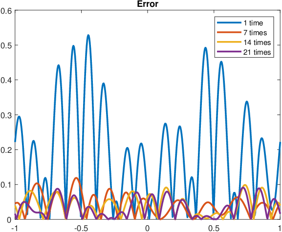
The graph of $\dot{q}$ is shown in Figure 3. The measurement $\dot{\Lambda}_{\dot{q}}$ is added with $0\%,1\%$ , and $5\%$ of Gaussian noise, respectively. The reconstructions and the corresponding errors are illustrated in Figure 3. Notice that the reconstruction error with $5\%$ noise is relatively larger, as can be expected. When multiple measurements are available, we can repeat the reconstruction several times and then take the average. This strategy effectively reduces the error, since the inverse problem is linear and the Gaussian noise have zero mean, see Figure 3.

Refer to caption — Figure 1: Ground truth $\dot{q}=\sin(\pi x)+2\cos(2\pi x)+4\sin(4\pi x)-3$ .

Experiment 2. The second experiment tests reconstruction of a discontinuous $\dot{q}$ . we choose $\dot{q}$ to be the Heaviside function

H(x)=\begin{cases}1&x\geq 0,\\ 0&x<0.\end{cases}

The Fourier series of $H(x)$ on $\Omega=[-1,1]$ is

H(x)=\frac{1}{2}+\sum_{n=1}^{\infty}\frac{2}{(2n-1)\pi}\sin((2n-1)\pi x).

With the choice of the finite computational basis, we can only expect to reconstruct the following orthogonal projection:

H_{N}(x):=\frac{1}{2}+\sum_{n=1}^{\left\lceil\frac{N}{2}\right\rceil}\frac{2}{(2n-1)\pi}\sin((2n-1)\pi x),

see Figure 6 for the graph of $H(x)$ and $H_{N}(x)$ . The reconstruction formula (24) is implemented with $0\%,1\%$ , and $5\%$ of Gaussian noise added to $\dot{\Lambda}_{\dot{q}}$ , respectively. The reconstructions and corresponding errors with a single measurement are illustrated in Figure 6. The averaged reconstruction with $5\%$ of Gaussian noise and multiple repeated measurements are illustrated in Figure 6.

Experiment 3. In this experiment, we apply the reconstruction formula (24) to measurement from the non-linear IBVP. Specifically, we choose $c_{0}=1$ and the potential

q=q_{0}+\varepsilon\dot{q}+\varepsilon^{2}\ddot{q}

where $\epsilon>0$ is a small number, the background potential $q_{0}=0$ , and the perturbations

\dot{q}=\sin(\pi x)+2\cos(2\pi x)+4\sin(4\pi x)-3,\qquad\ddot{q}=20\cos(20\pi x).

We apply the reconstruction formula (24), with $\dot{\Lambda}_{\dot{q}}f$ replaced by $\Lambda_{q}f-\Lambda_{q_{0}}f$ (where $\Lambda_{q}f$ and $\Lambda_{q_{0}}f$ are computed by solving the boundary value problem (1)), and then add $q_{0}$ to the reconstruction to obtain an approximation of $q$ . The rationale is that, when $\epsilon$ is small, we have the following approximation

\Lambda_{q}-\Lambda_{q_{0}}\approx\varepsilon\dot{\Lambda}_{\dot{q}}=\dot{\Lambda}_{\epsilon\dot{q}}.

Therefore, the resulting reconstruction from (24) is approximately $\epsilon\dot{q}$ , and adding $q_{0}$ to it yields a linear approximation of $q$ . We choose $\epsilon=0.1$ . The ground truth is illustrated in Figure 9.

Adding noise is a bit delicate in this experiment. The noise to be added is additive and proportional to the magnitude of the signal. We tested two ways of adding noise: (1) adding noise to the difference $(\Lambda_{q}-\Lambda_{q_{0}})f$ ; (2) adding noises to $\Lambda_{q}f$ and $\Lambda_{q_{0}}f$ respectively, then subtract to find the difference. The resulting numerical performance are different, and it turns out the former introduces much less error than the latter. This is because the numerical values in the discretization of $(\Lambda_{q}-\Lambda_{q_{0}})f$ are much smaller, hence the proportional noise is relatively small. In contrast, the numerical values in the discretization of $\Lambda_{q}f$ and $\Lambda_{q_{0}}f$ are larger, hence the proportional noise is relatively large. Comparison of the reconstruction errors are shown in Figure 9 and Figure 9. Note that the noise added in Figure 9 (0.1% and 0.5%) is only a tenth of that in Figure 9 (1% and 5%).

Acknowledgment

The research of T. Yang and Y. Yang is partially supported by the NSF grant DMS-1715178, DMS-2006881, and startup fund from Michigan State University.

Appendix

In this appendix, we collect a few results that are used in the main text. First, we present a lemma regarding uniform continuity of min/max functions, which is used in the proof of Proposition 4.

Lemma 10.

Let $X,Y$ be compact metric spaces and suppose that $f:X\times Y\to\mathbb{R}$ is uniformly continuous. Then the function $F:X\to\mathbb{R}$

\displaystyle F(x):=\min\{f(x,y):y\in Y\}

is uniformly continuous. The same is true if $\min$ is replaced by $\max$ .

Proof.

Let $\epsilon>0$ and let $x,x^{\prime}\in X$ . We may assume without loss of generality that $F(x)\geq F(x^{\prime})$ . Let $y,y^{\prime}\in Y$ be such that $F(x)=f(x,y)$ and $F(x^{\prime})=f(x^{\prime},y^{\prime})$ , then

\displaystyle|F(x)-F(x^{\prime})|=f(x,y)-f(x^{\prime},y^{\prime})\leq f(x,y^{\prime})-f(x^{\prime},y^{\prime})

Due to uniform continuity there is $\delta>0$ such that

\displaystyle|f(x,y^{\prime})-f(x^{\prime},y^{\prime})|<\epsilon

whenever $d(x,x^{\prime})<\delta$ . The proof when “ $\min$ ” is replaced by “ $\max$ ” is similar. ∎

Next, we construct a Helmholtz solution of the form (25), with $r$ satisfying the asymptotic condition (26).

Lemma 11.

Let $\lambda\geq 0$ . The perturbed Helmholtz equation $(\Delta+\lambda-q_{0})\phi=0$ admits solutions of the form

\phi(x)=e^{i\sqrt{\lambda}\theta\cdot x}+r(x;\lambda)

for any $\theta\in\mathbb{S}^{n-1}$ , with $\|r\|_{H^{s}(\mathbb{R}^{n})}=O(\lambda^{\frac{s-1}{2}})$ as $\lambda\rightarrow\infty$ for any $s\geq 0$ .

Proof.

If $\phi(x)=e^{i\sqrt{\lambda}\theta\cdot x}+r(x;\lambda)$ solves the perturbed Helmholtz equation and $\theta\in\mathbb{S}^{n-1}$ , then $r$ has to satisfy

(\Delta+\lambda-q_{0})r=q_{0}e^{i\sqrt{\lambda}\theta\cdot x}\quad\quad\text{ in }\Omega.

(29)

Such $r$ can be constructed as follows. Let $R(\lambda):=(\Delta+\lambda-q_{0})^{-1}$ be the outgoing resolvent of the perturbed Helmholtz operator. For any compactly supported smooth function $\chi\in C^{\infty}_{c}(\mathbb{R}^{n})$ , the following $L^{2}$ -resolvent estimate holds [17, Theorem 3.1]:

\|\chi R(\lambda)\chi\|_{L^{2}(\mathbb{R}^{n})\rightarrow L^{2}(\mathbb{R}^{n})}\leq\frac{C}{\sqrt{\lambda}}

(30)

where $C>0$ is a constant independent of $\lambda$ . In particular, we choose $\chi\in C^{\infty}_{c}(\mathbb{R}^{n})$ such that $\chi=1$ on $\overline{\Omega}$ and set $r:=\chi R(\lambda)\chi(q_{0}e^{i\sqrt{\lambda}\theta\cdot x})$ , then $r$ satisfies (29), $r$ is compactly supported, and

\|r\|_{L^{2}(\mathbb{R}^{n})}\leq\frac{C}{\sqrt{\lambda}}.

(31)

This proves the claim when $s=0$ .

We proceed by induction. Suppose it has been proved that $r$ is compactly supported and satisfies $\|r\|_{H^{s}(\mathbb{R}^{n})}=O(\lambda^{\frac{s-1}{2}})$ as $\lambda\rightarrow\infty$ for some integer $s\geq 0$ . Let $\Omega_{1}$ , $\Omega_{2}$ be two open sets such that $\Omega\subset\text{supp}\,\chi\subset\Omega_{1}\subset\overline{\Omega_{1}}\subset\Omega_{2}$ . We apply the interior regularity estimate [20, Section 6.3, Theorem 2 ] to the equation $(\Delta-q_{0})r=q_{0}e^{i\sqrt{\lambda}\theta\cdot x}-\lambda r$ to obtain

	$\displaystyle\\|r\\|_{H^{s+2}(\mathbb{R}^{n})}=\\|r\\|_{H^{s+2}(\Omega_{1})}$	$\displaystyle\leq C\left(\\|q_{0}e^{i\sqrt{\lambda}\theta\cdot x}-\lambda r\\|_{H^{s}(\Omega_{2})}+\\|r\\|_{H^{s}(\Omega_{2})}\right)$
		$\displaystyle\leq C\left(1+\lambda\\|r\\|_{H^{s}(\mathbb{R}^{n})}+\\|r\\|_{H^{s}(\mathbb{R}^{n})}\right)\leq C(1+\lambda^{\frac{s+1}{2}}).$

This completes the inductive step, hence the claim holds for all even integers $s$ . The general claim is a consequence of interpolation. ∎

References

[1] S. Alexakis, A. Feizmohammadi, and L. Oksanen. Lorentzian Calderón problem near the minkowski geometry, 2021.
[2] M. Anderson, A. Katsuda, Y. Kurylev, M. Lassas, and M. Taylor. Boundary regularity for the Ricci equation, geometric convergence, and Gel’fand’s inverse boundary problem. Invent. Math., 158(2):261–321, 2004.
[3] M. Belishev. On an approach to multidimensional inverse problems for the wave equation. In Soviet Math. Dokl, volume 36, pages 481–484, 1988.
[4] M. Belishev and V. Y. Gotlib. Dynamical variant of the bc-method: theory and numerical testing. Journal of Inverse and Ill-Posed Problems, 7(3):221–240, 1999.
[5] M. I. Belishev. Recent progress in the boundary control method. Inverse Problems, 23(5):R1–R67, 2007.
[6] M. I. Belishev, I. B. Ivanov, I. V. Kubyshkin, and V. S. Semenov. Numerical testing in determination of sound speed from a part of boundary by the bc-method. Journal of Inverse and Ill-posed Problems, 24(2):159–180, 2016.
[7] M. I. Belishev and Y. V. Kuryiev. To the reconstruction of a Riemannian manifold via its spectral data (bc–method). Communications in partial differential equations, 17(5-6):767–804, 1992.
[8] M. Bellassoued and D. D. S. Ferreira. Stability estimates for the anisotropic wave equation from the Dirichlet-to-Neumann map. Inverse Problems and Imaging, 5(4):745–773, 2011.
[9] K. Bingham, Y. Kurylev, M. Lassas, and S. Siltanen. Iterative time-reversal control for inverse problems. Inverse Problems & Imaging, 2(1):63, 2008.
[10] A. Blagoveshchenskii. The inverse problem in the theory of seismic wave propagation. In Spectral Theory and Wave Processes, pages 55–67. Springer, 1967.
[11] E. Blåsten, F. Zouari, M. Louati, and M. S. Ghidaoui. Blockage detection in networks: The area reconstruction method. arXiv preprint arXiv:1909.05497, 2019.
[12] R. Bosi, Y. Kurylev, and M. Lassas. Reconstruction and stability in Gel’fand’s inverse interior spectral problem, 2019.
[13] D. Burago, S. Ivanov, M. Lassas, and J. Lu. Stability of the Gel’fand inverse boundary problem via the unique continuation, 2021.
[14] E. Burman, A. Feizmohammadi, A. Munch, and L. Oksanen. Spacetime finite element methods for control problems subject to the wave equation. arXiv preprint arXiv:2109.07890, 2021.
[15] M. V. De Hoop, P. Kepley, and L. Oksanen. An exact redatuming procedure for the inverse boundary value problem for the wave equation. SIAM Journal on Applied Mathematics, 78(1):171–192, 2018.
[16] M. V. de Hoop, P. Kepley, and L. Oksanen. Recovery of a smooth metric via wave field and coordinate transformation reconstruction. SIAM Journal on Applied Mathematics, 78(4):1931–1953, 2018.
[17] S. Dyatlov and M. Zworski. Mathematical theory of scattering resonances, volume 200. American Mathematical Soc., 2019.
[18] S. Ervedoza, E. Zuazua, et al. A systematic method for building smooth controls for smooth data. 2010.
[19] G. Eskin. Inverse hyperbolic problems with time-dependent coefficients. Communications in Partial Differential Equations, 32(11):1737–1758, 2007.
[20] L. C. Evans. Partial differential equations. Graduate studies in mathematics, 19(4):7, 1998.
[21] A. Katchalov, Y. Kurylev, and M. Lassas. Inverse boundary spectral problems, volume 123 of Chapman & Hall/CRC Monographs and Surveys in Pure and Applied Mathematics. Chapman & Hall/CRC, Boca Raton, FL, 2001.
[22] J. Korpela, M. Lassas, and L. Oksanen. Discrete regularization and convergence of the inverse problem for 1+1 dimensional wave equation. Inverse Problems & Imaging, 13(3):575–596, 2019.
[23] Y. Kurylev. An inverse boundary problem for the Schrödinger operator with magnetic field. J. Math. Phys., 36(6):2761–2776, 1995.
[24] Y. Kurylev and M. Lassas. Gelf’and inverse problem for a quadratic operator pencil. J. Funct. Anal., 176(2):247–263, 2000.
[25] Y. Kurylev, L. Oksanen, and G. P. Paternain. Inverse problems for the connection Laplacian. J. Differential Geom., 110(3):457–494, 2018.
[26] S. Liu and L. Oksanen. A lipschitz stable reconstruction formula for the inverse problem for the wave equation. Transactions of the American Mathematical Society, 368(1):319–335, 2016.
[27] C. Montalto. Stable determination of a simple metric, a covector field and a potential from the hyperbolic Dirichlet-to-Neumann map. Communications in Partial Differential Equations, 39(1):120–145, 2014.
[28] L. Oksanen. Solving an inverse obstacle problem for the wave equation by using the boundary control method. Inverse Problems, 29(3):035004, 2013.
[29] L. Pestov, V. Bolgova, and O. Kazarina. Numerical recovering of a density by the bc-method. Inverse Problems & Imaging, 4(4):703, 2010.
[30] Rakesh and W. W. Symes. Uniqueness for an inverse problem for the wave equation: Inverse problem for the wave equation. Communications in Partial Differential Equations, 13(1):87–96, 1988.
[31] P. Stefanov and G. Uhlmann. Stability estimates for the hyperbolic Dirichlet to Neumann map in anisotropic media. journal of functional analysis, 154(2):330–358, 1998.
[32] P. Stefanov and G. Uhlmann. Stable determination of generic simple metrics from the hyperbolic Dirichlet-to-Neumann map. International Mathematics Research Notices, 2005(17):1047–1061, 2005.
[33] P. Stefanov and Y. Yang. The inverse problem for the Dirichlet-to-Neumann map on Lorentzian manifolds. Analysis & PDE, 11(6):1381–1414, 2018.
[34] P. D. Stefanov. Uniqueness of the multi-dimensional inverse scattering problem for time dependent potentials. Mathematische Zeitschrift, 201(4):541–559, 1989.
[35] Z. Sun. On continuous dependence for an inverse initial boundary value problem for the wave equation. Journal of Mathematical Analysis and Applications, 150(1):188–204, 1990.
[36] D. Tataru. Unique continuation for solutions to PDE’s; between Hormander’s theorem and Holmgren’s theorem. Communications in Partial Differential Equations, 20(5-6):855–884, 1995.
[37] T. Yang and Y. Yang. A stable non-iterative reconstruction algorithm for the acoustic inverse boundary value problem. Inverse Problems & Imaging, 2021.

	$\displaystyle I(T,T)$	$\displaystyle=\frac{1}{2}\int^{T}_{0}\int^{2T-t}_{t}\left[(f(t),\Lambda_{q}P^{}_{T}h(\sigma))_{L^{2}(\partial\Omega)}-(\Lambda_{q}P^{}_{T}f(t),h(\sigma))_{L^{2}(\partial\Omega)}\right]\,d\sigma dt\vskip 4.30554pt$
		$\displaystyle=\int^{T}_{0}[(f(t),\frac{1}{2}\int^{2T-t}_{t}\Lambda_{q}P^{}_{T}h(\sigma)\,d\sigma)_{L^{2}(\partial\Omega)}-(\Lambda_{q}P^{}_{T}f(t),\frac{1}{2}\int^{2T-t}_{t}h(\sigma)\,d\sigma)_{L^{2}(\partial\Omega)}]\,dt\vskip 4.30554pt$
		$\displaystyle=(f,J\Lambda_{q}P^{}_{T}h)_{L^{2}((0,T)\times\partial\Omega)}-(P_{T}(\Lambda_{q}f),JP^{}_{T}h)_{L^{2}((0,T)\times\partial\Omega)}.$

	$\displaystyle\left\|\mathcal{F}[\dot{q}](\sqrt{2\lambda}\theta)\right\|\leq$	$\displaystyle\\|\partial^{2}_{t}f+\lambda f\\|_{L^{2}((0,T)\times\partial\Omega)}\\|h\\|_{L^{2}((0,T)\times\partial\Omega)}\\|\dot{K}\\|_{L^{2}((0,T)\times\partial\Omega)\rightarrow L^{2}((0,T)\times\partial\Omega)}$
	$\displaystyle+$	$\displaystyle\\|\dot{\Lambda}f(T)\\|_{L^{2}(\partial\Omega)}\\|h(T)\\|_{L^{2}(\partial\Omega)}$
	$\displaystyle\leq$	$\displaystyle(1+\lambda)\\|f\\|_{H^{2}((0,T)\times\partial\Omega)}\\|h\\|_{L^{2}((0,T)\times\partial\Omega)}\\|\dot{K}\\|_{L^{2}((0,T)\times\partial\Omega)\rightarrow L^{2}((0,T)\times\partial\Omega)}$
	$\displaystyle+$	$\displaystyle\\|\dot{\Lambda}f\\|_{H^{1}((0,T)\times\partial\Omega)}\\|h\\|_{H^{1}((0,T)\times\partial\Omega)}$

	$\displaystyle\left\|\mathcal{F}[\dot{q}](\sqrt{2\lambda}\theta)\right\|\leq$	$\displaystyle(1+\lambda)\\|f\\|_{H^{2}((0,T)\times\partial\Omega)}\\|h\\|_{H^{1}((0,T)\times\partial\Omega)}\\|\dot{K}\\|_{L^{2}((0,T)\times\partial\Omega)\rightarrow L^{2}((0,T)\times\partial\Omega)}$
	$\displaystyle+$	$\displaystyle\\|\dot{\Lambda}f\\|_{H^{3}((0,T)\times\partial\Omega)}\\|h\\|_{H^{1}((0,T)\times\partial\Omega)}$
	$\displaystyle\leq$	$\displaystyle(1+\lambda)\\|f\\|_{H^{2}((0,T)\times\partial\Omega)}\\|h\\|_{H^{1}((0,T)\times\partial\Omega)}\\|\dot{K}\\|_{L^{2}((0,T)\times\partial\Omega)\rightarrow L^{2}((0,T)\times\partial\Omega)}$
	$\displaystyle+$	$\displaystyle\\|f\\|_{H^{2}((0,T)\times\partial\Omega)}\\|\dot{\Lambda}\\|_{H^{2}((0,T)\times\partial\Omega)\rightarrow H^{3}((0,T)\times\partial\Omega)}\\|h\\|_{H^{1}((0,T)\times\partial\Omega)}$
	$\displaystyle\leq$	$\displaystyle C_{\lambda}\left(\\|\dot{K}\\|_{L^{2}((0,T)\times\partial\Omega)\rightarrow L^{2}((0,T)\times\partial\Omega)}+\\|\dot{\Lambda}\\|_{H^{2}((0,T)\times\partial\Omega)\rightarrow H^{3}((0,T)\times\partial\Omega)}\right)$

	$\displaystyle\|\hat{\dot{q}}(\xi)\|$	$\displaystyle\leq\|(\partial^{2}_{t}f+(k^{2}+l^{2}),\dot{K}h)_{L^{2}((0,T)\times\partial\Omega)}+(\dot{\Lambda}f(T),h(T))_{L^{2}(\partial\Omega)}\|+\frac{C}{\sqrt{\lambda}}$
		$\displaystyle\leq C(2+\lambda)\\|\phi\\|_{H^{4}(\Omega)}\\|\psi\\|_{H^{4}(\Omega)}\delta+\frac{C}{\sqrt{\lambda}}$
		$\displaystyle\leq C(2+\lambda)\left(\\|\phi_{0}\\|_{H^{4}(\Omega)}+\\|r_{1}\\|_{H^{4}(\Omega)}\right)\left(\\|\psi_{0}\\|_{H^{4}(\Omega)}+\\|r_{2}\\|_{H^{4}(\Omega)}\right)\delta+\frac{C}{\sqrt{\lambda}}$
		$\displaystyle\leq C(2+\lambda)\left(\lambda^{2}+\lambda^{\frac{3}{2}}\right)^{2}\delta+\frac{C}{\sqrt{\lambda}}$

A Linearized Boundary Control Method for the Acoustic Inverse Boundary Value Problem

Abstract

1 Introduction

2 Preliminaries

Proposition 1.

Proof.

Corollary 2.

Proof.

3 Integral Identity and Controllability

Proposition 3.

Proof.

Proposition 4.

Proof.

4 Stability and Reconstruction

4.1 Case 1: c0=1c_{0}=1 and q0=0q_{0}=0

Theorem 5.

Proof.

Remark 6.

Theorem 7.

Proof.

4.2 Case 2: c0=1c_{0}=1 and q0≠0q_{0}\neq 0

Theorem 8.

Proof.

Theorem 9.

Proof.

5 Numerical Experiments

5.1 Computing Boundary Controls with Time Reversal

5.2 Numerical Experiments

Acknowledgment

Appendix

Lemma 10.

Proof.

Lemma 11.

Proof.

References

4.1 Case 1: $c_{0}=1$ and $q_{0}=0$

4.2 Case 2: $c_{0}=1$ and $q_{0}\neq 0$