Determining the Hubble constant without the sound horizon: Perspectives with future galaxy surveys
Abstract
constraints from galaxy surveys are sourced by the geometric properties of two standardisable rulers: the sound horizon scale, , and the matter-radiation equality scale, . While most analyses over the past decade have focused on the first scale, recent work has emphasised that the second can provide an independent source of information about the expansion rate of the universe. In this work, we demonstrate an improved method for performing such a measurement with future galaxy surveys such as Euclid. Previous approaches have avoided -based information by removing the prior on the baryon density, and thus the sound-horizon calibration. Here, we present a new method to marginalise over ; this allows baryon information to be retained, which enables tighter parameter constraints. For a Euclid-like spectroscopic survey, we forecast sound-horizon independent constraints of for our method using the equality scale, compared with from the sound horizon. Upcoming equality scale measurements thus can be highly competitive, although we caution that the impact of observational systematics on such measurements still needs to be investigated in detail. Applying our new approach to the BOSS power spectrum gives from equality alone, somewhat tighter than previous constraints. Consistency of - and -based measurements can provide a valuable internal consistency test of the cosmological model; as an example, we consider the change in created by early dark energy. Assuming the Planck+SH0ES best-fit early dark energy model we find a shift () between the two measurements for Euclid; if we instead assume the ACT best-fit model, this increases to ().
I Introduction
The Hubble parameter encodes the Universe’s expansion rate and sets the scale of the cosmos. One of the most discussed problems in cosmology today is that two of the most precise measurements of the Hubble constant are in disagreement. In particular, constraints derived from the Cosmic Microwave Background (CMB) power spectrum give (Planck Collaboration et al. 2020, e.g.,), whereas local, direct, measurements of the expansion from Cepheid-calibrated supernovae give (Riess et al. 2019; Schombert et al. 2020; Riess et al. 2021a; Riess et al. 2021b, e.g.,). The tension between these two measurements has reached high significance ( with the most recent Planck Planck Collaboration et al. 2020 and SH0ES Riess et al. 2021b measurements), motivating a wealth of experimental and theoretical activity to resolve this apparent problem.
Of course, CMB and Cepheid-calibrated local measurements are not the only methods by which can be constrained; in particular, large-scale structure has recently emerged as a competitive probe of the expansion rate, using several methods (Alam et al. 2017; Cuceu et al. 2019; Abbott et al. 2018; Aylor et al. 2019; Schöneberg et al. 2019; Addison et al. 2018; Colas et al. 2020; eBOSS Collaboration et al. 2020; d’Amico et al. 2020; Philcox et al. 2020; Zhang et al. 2021; Chen et al. 2021, e.g.,). All the measurements that are indirect (relying on a cosmological model depending on physics from both low and high redshifts) give . The direct measurements are somewhat less consistent: those calibrated from stellar modeling (i.e. tip of the red giant branch stars) fall somewhat lower than the Cepheid results (Riess et al. 2021a; Freedman et al. 2019), and, while strong lensing had previously favored a higher value, a detailed treatment of uncertainties in the mass density profiles has made this less certain (Birrer et al. 2020). Until recently, indirect measurements all had one thing in common: they derived their constraints from measurements of the angular scale (or redshift separation) of the sound horizon scale at photon-baryon decoupling (), which was assumed to be computable via standard CDM physics.11 1 For the purposes of this work, there is little difference between ‘recombination’ and ‘decoupling’; we thus use the terms interchangeably.
This observation has led to some of the best-motivated theoretical attempts to resolve the so-called Hubble tension: invoking a mechanism that changes the sound horizon scale, , in the early Universe. However, several hundred such models have now been proposed Knox and Millea 2020; Di Valentino et al. 2021; arguably, none are perfectly well motivated, natural, and able to consistently fit the wealth of cosmological data available Hill et al. 2020; Hill et al. 2021. Whilst one possible approach is to try and constrain each proposed model individually, we believe that this zoo of possible theories motivates the development of general diagnostics that are sensitive to such -varying models.
Our previous work Baxter and Sherwin 2020; Philcox et al. 2020 proposed one such consistency test: a method to measure the Hubble constant that does not rely on , but instead makes use of another scale imprinted in the large-scale structure, namely the matter-radiation equality scale, , corresponding to the size of the horizon when the density of matter and radiation were equal, at . This scale can be given approximately within the CDM model as
| (1) |
(Eisenstein and Hu 1998; Chudaykin and Ivanov 2019) so that when measured in units of . Most directly, sets the scale of the matter and galaxy power spectrum peak, but it also is encoded in the full shape of the spectrum around the peak (as well as, logarithmically, in the spectrum shape at higher ). Therefore, even though resolving the peak itself is generally difficult in galaxy surveys, can still be inferred from somewhat smaller (though still linear) scales as discussed in Ref. Philcox et al. 2020. If observational systematic uncertainties arising, for example, from spatially varying sample completeness can be controlled on the relevant scales, can hence be constrained from the galaxy power spectrum.
Previously, our method avoided making use of information from by carefully choosing which sources of information to omit; in particular, by ensuring that our LSS analyses did not use a prior on the baryon density (unlike standard approaches), we showed that the sound horizon remained uncalibrated and hence uninformative. Of course, omitting sources of information invariably degrades the achievable constraints, which was an unfortunate feature of our method.
In this paper, we develop an analysis technique that avoids unnecessary degradation of our constraints by directly marginalising over templates that capture the power spectrum features encoding the sound horizon scale, namely oscillatory baryon acoustic oscillation (BAO) features and a broadband baryonic suppression. Using this framework, we are free to add additional sources of information, such as priors on the baryon density, which helps to maximise the constraining power of our new ‘standardisable ruler’, .
We demonstrate our method in a mock analysis of the Euclid spectroscopic data, forecasting the expected constraints, and also apply it to current BOSS data. Furthermore, we discuss the power of this method to constrain new physics models, using the example of early dark energy (EDE) Poulin et al. 2019; Smith et al. 2020; Lin et al. 2019; Lin et al. 2020; Sakstein and Trodden 2020; Niedermann and Sloth 2021a; Hill et al. 2021. This was recently advocated as a possible resolution to the so-called Hubble tension, though this is disputed when galaxy survey data is also included Hill et al. 2020; Ivanov et al. 2020; D’Amico et al. 2021; Niedermann and Sloth 2021b; Smith et al. 2021.
Our paper is organised as follows. In §II we introduce our method for marginalising over the sound horizon, which is tested in §III, using a mock-based Euclid forecast. §IV discusses how our new prescription can be used to test for new physics models. §V presents constraints with current BOSS galaxy data, before we conclude in §VI. Appendices A-C give supplementary details relating to our procedure to marginalise over broadband information, ‘de-wiggled’ constraint plots, and discussion of the dependence of our results on wavenumber and redshift cuts.
II Measuring via -marginalisation
As previously discussed, the most promising approaches for cosmological resolutions to the so-called Hubble tension involve changing the physical size of the sound horizon, , at photon-baryon decoupling. The large-scale distribution of matter exhibits two features controlled by . Primarily, controls the BAO scale observable from the large scale structure (LSS) power spectrum through the spacing of the characteristic oscillatory feature. Additionally, controls the broadband baryon suppression scale, which suppresses the power spectrum on scales smaller than the sound horizon.
Given knowledge of the physical size of the sound horizon, one can use the observed angular scale of the BAO feature to constrain the Universe’s expansion history. As discussed in §I, our desire in this work is to avoid using this information to constrain , instead making use of the second scale available from the power spectrum; the horizon size at matter-radiation equality, . The sound horizon, , is not a direct input to the theory computation but rather an emergent quantity determined within a given cosmological model by integrating the sound speed, , in the photon-baryon plasma up to decoupling
| (2) |
Hence, one cannot directly marginalise over it. However, we show here that such a marginalisation can be performed heuristically, by scaling the spacing of the BAO wiggles.22 2 We return to the issue of broadband suppression below. While such a rescaling is not physical (i.e. the rescaled spectra do not satisfy the perturbation equations), this is allowable: our marginalisation is a conservative approach that effectively integrates over any phenomenon capable of rescaling the BAO feature, whether or not it is allowed by physical arguments.
To implement this, we first split the power spectrum into ‘wiggly’ and ‘non-wiggly’ pieces, denoted and respectively. Such a decomposition is already necessary for the process of infrared resummation (the treatment of long wavelength displacements needed for accurate perturbative modeling of the the BAO feature Ivanov and Sibiryakov 2018; Chudaykin et al. 2020). This separates out the physical contributions: information about the BAO wiggle spacing (and thus ) appears in the ‘wiggly’ part, while the ‘non-wiggly’ component contains information from the equality scale. We can thus effectively marginalise over the sound horizon by introducing a scaling parameter to the ‘wiggly’ component only, making the replacement
| (3) |
Notably, we perform this operation on the linear power spectrum. This is in contrast to traditional BAO analyses, which rescale the nonlinear power spectrum; we use this approach since we are interested in marginalising over a change in the physical size of the sound horizon rather than an Alcock-Paczynski scaling from cosmological coordinate conversion.
The convolution integrals relevant for the postlinear order terms in the power spectrum model (cf. §III.1) are then evaluated using this modified linear power spectrum, . This is performed using CLASS-PT, a modified version of the Boltzmann code CLASS that has has been augmented with a perturbation theory treatment of nonlinear structure formation (see Ref. Chudaykin et al. 2020 for details). We have further extended this to implement the above -marginalisation procedure.33 3 CLASS-PT is available online here: GitHub.com/Michalychforever/CLASS-PT and our modified version may be accessed at GitHub.com/gerrfarr/CLASS-PT. Within CLASS-PT separation of the power spectrum components is performed in the following way. First, the spectrum is transformed to position space via a discrete sine transform, the BAO feature is removed and the resulting correlation function is smoothly interpolated (cf. §4 of Ref. Chudaykin et al. 2020). Converting back to momentum space one obtains the ‘non-wiggly’ power spectrum. The ‘wiggly’ part (before -rescaling) is equal to the difference between the initial linear power spectrum and the ‘non-wiggly’ part, .
Fig. 1 shows model nonlinear power spectra for different values of . One can clearly observe that the action of the rescaling parameter is to shift the characteristic BAO wiggles, as required. On scales the wiggly feature is strongly suppressed, thus the rescaled spectra agree with the fiducial one, as expected. In §III we discuss our nonlinear power spectrum model, free parameters and fiducial assumptions in more detail.
The baryon suppression scale provides a second source of information about , which is nonoscillatory, and will thus not be marginalised over by the above prescription. Instead, we adopt an approximate procedure to remove the information, using a method similar to that applied to nuisance parameter marginalisation in Refs. Chudaykin and Ivanov 2019; Philcox et al. 2020. To motivate this, we consider some parameter , with a Gaussian prior of mean and width , entering our model vector linearly. This can be exactly marginalised over by evaluating at , and modifying the data covariance as follows Taylor and Kitching 2010:
| (4) |
While the nonlinear power spectrum clearly does not depend linearly on a rescaling of the baryon suppression scale (denoted by ), we can Taylor expand our model to first order in this rescaling
| (5) |
An approximate marginalisation at lowest order is thus possible analytically even for nonlinear dependencies. In principle one might envision using a similar procedure to also marginalise over the BAO feature in the power spectrum. However, in practice the linear approximation breaks down even for relatively small rescalings of the oscillatory BAO feature. The much smoother power spectrum features associated with the baryon suppression scale are more accurately approximated by a linear order expansion.44 4 In initial testing, the BAO feature was marginalised over via this method, obtaining model derivatives using the analytic Eisenstein-Hu model Eisenstein and Hu 1998 as described here for the baryon suppression scale. This method was not able to achieve constraints largely independent of and hence we adopted the approach described in the main text.
To obtain the relevant derivatives in practice, we consider the analytic Eisenstein-Hu transfer function (Eisenstein and Hu 1998). This model smoothly interpolates between an unsuppressed transfer function and a baryon-suppressed transfer function near the sound horizon scale using
| (6) |
where for empirical constants and . To rescale the suppression scale we make the replacement . Given this modified linear power spectrum, we differentiate our full nonlinear model with respect to numerically, using a five-point, finite difference rule. In Appendix A we demonstrate, however, that, at least for a Euclid-like survey with our current modeling choices, the impact of the broadband-derived information is negligible, so that we can ignore it for the remainder of our paper.
III Method Verification and Euclid Forecasts
In this section, we present the results of Markov chain Monte Carlo (MCMC) analyses, which aim to demonstrate that the method described in §II can produce -independent constraints on . Furthermore, we demonstrate that for future spectroscopic surveys such as Euclid, such constraints will be competitive with those from other probes.
III.1 Power spectrum model
Given that one of the goals of this paper is to provide a partially model-independent test for various cosmological models that propose solutions to the so-called Hubble tension, we fix our baseline cosmology to the best fit CDM model from Ref. Smith et al. 2020, which will allow us to later contrast the results with their best fit early dark energy (EDE) model. Explicitly, our fiducial cosmology is given by
We also include a single massive neutrino species with mass .
Our standard analysis assumes a Euclid-like spectroscopic survey, and models the power spectrum using the effective field theory of LSS. This features a consistent one-loop perturbative model, including ultraviolet counterterms, infrared resummation, Alcock-Paczynski distortions and Fingers-of-God corrections (Ivanov et al. 2020; d’Amico et al. 2020; Chen et al. 2021, cf.,). Our power spectrum model contains nine nuisance parameters: the linear, quadratic, tidal and cubic tidal bias parameters (, , and ), the monopole, quadrupole and hexadecapole counterterms (, and ), and two stochastic contributions, ( and ), scaling as and respectively. For details, we refer the reader to Refs. Chudaykin et al. 2020; Ivanov et al. 2020, or Ref. Chudaykin and Ivanov 2019, for those pertaining to Euclid. We additionally assume a Gaussian likelihood, with a theoretical covariance matrix, encoding both cosmic variance and theoretical uncertainties, following Ref. Chudaykin and Ivanov 2019.
The survey is specified by eight nonoverlapping redshift bins evenly spaced between and . Within each redshift bin we analyse the monopole, quadrupole and hexadecapole in 40 bins evenly spaced in between (matching past BOSS analyses) and . In addition to our cosmological parameters (and where relevant the sound horizon marginalisation parameter, ), we include a total of 72 nuisance parameters (nine for each redshift slice). To reduce the dimensionality of our parameter space, we analytically marginalise over any parameter that enters our model linearly (Chudaykin and Ivanov 2019; Philcox et al. 2020); these are the counterterm parameters, the stochasticity parameters, and the cubic tidal bias parameters. This procedure is exact and equivalent to numerical marginalisation with Gaussian priors Taylor and Kitching 2010. The remaining bias parameters, , and , are allowed to vary freely, though we impose Gaussian priors of width on the latter two, centred on the true values.
Mock power spectrum data are generated using the following fiducial values for the nuisance parameters:
| (7) |
where is an estimate of the number density of galaxies observed in each redshift bin and is the scale independent growth rate computed with our fiducial cosmology. Note that the values adopted for the counterterm parameters are based on fits to the eBOSS ELG sample Ivanov 2021, rather than those presented in Ref. Chudaykin and Ivanov 2019. We do not expect the fiducial choice for these nuisance parameters to significantly affect our forecasts. The fiducial numeric values for all nuisance parameters are shown in Table 1. Furthermore, we note that no BAO reconstruction is included in this analysis; this would further tighten the -based constraints. We do not include noise in our mock data.
| 267 | |||||||||||
| 493 | |||||||||||
| 872 | |||||||||||
| 1484 | |||||||||||
| 2643 | |||||||||||
| 4943 | |||||||||||
| 8865 | |||||||||||
| 15323 |
III.2 Parameter recovery and forecasts
Reference Philcox et al. 2020 noted that -independent constraints can be derived from a full shape (FS) galaxy power spectrum analysis when calibration of the BAO feature is explicitly avoided, by removing prior information on the baryon density, . In our analyses, we can either omit this prior as before or include it while marginalising over ; we present results from a full MCMC analysis for both cases.
| FS | |
|---|---|
| FS + marg. | |
| FS + BBN | |
| FS + BBN + marg. | |
| BAO + BBN | |
| BAO + BBN + marg |
Results from the various MCMC analyses are shown in Fig. 2 and Table 2. First, we consider the results obtained using the previous prescription: when performing an analysis without a baryon prior or -marginalisation, we obtain a measurement of (), in good agreement with our earlier forecast. The omission of such a prior, however, not only removes information from the BAO scale but also reduces the information that can be extracted from other features of the FS power spectrum. Figure 4a shows a clear degeneracy between and even for the -marginalised analysis. This is not unexpected; clearly any additional information on will directly improve constraint on (and thus in units). Additionally, the amplitudes of the BAO peaks, for example, are sensitive to the ratio of baryons to dark matter and can thus be used to sharpen the constraint on further if information about the baryon density is provided.
When a prior on the baryon density is included [specifically, a Gaussian prior of from big bang nucleosynthesis; BBN],55 5 This has the same fractional width as in Ref. Philcox et al. 2020. our forecasted constraint tightens to . However, this will now include information sourced by . Using the -marginalisation procedure described in §II (integrating over ), we can isolate the -based information (ignoring broadband suppression, which Appendix A finds to be negligible), which yields . This is substantially tighter than our analysis without BBN information, and shows the utility of our method. In §III.3 we demonstrate that this is indeed independent of . It should be noted that our constraints without the BBN prior are somewhat wider than those reported in Ref. Chudaykin and Ivanov 2019. This occurs since our work is based on an updated version of the relevant Euclid likelihood, which, for example, adds the scale-dependent stochastic contribution . Furthermore, we can quantify the information content of alone with a BAO-only forecast, akin to that done in traditional power spectrum analyses (Alam et al. 2017, e.g.). This is described in §III.3, and gives the constraint , somewhat stronger than the equality-based constraint. Notably, the combined constraint is approximately equal to the inverse-variance weighted mean of the two constraints, hinting at their independence. The fact that the BAO constraint is significantly tighter than the equality-derived constraint illustrates that the combined constraint is dominated by -derived information, with the -derived result obscured in the combination; -marginalisation is therefore necessary to isolate the equality-derived information.
As seen in Fig. 2, we obtain unbiased and consistent parameter recovery for all cosmological parameters both with and without a prior on . When applying our heuristic -marginalisation procedure without the prior we find only a very minor difference to the standard FS analysis (, ). This is expected given that sound horizon information should be subdominant in this analysis from the outset (since the standard ruler is uncalibrated).
III.3 independence
We now present a set of tests to validate the independence of our constraints from the sound horizon scale. This is necessary to ensure that we are indeed obtaining information from and that our constraints are not derived from residual -derived information. Three different tests are presented.
First, we compare to results from a BAO-only analysis, which does not include information from the broadband shape of the power spectrum. Next, we compare to Fisher forecasts including an exact marginalisation over the sound horizon, and, finally, inspect the degeneracy between the approximate sound horizon scale and . In Appendix B we also compare our analysis to one run on a dataset from which the BAO feature has been removed. We find a similar posterior, showing that such constraints can be derived from the broadband alone.
Furthermore, we explore the impact of scale and redshift selections in Appendix C using Fisher forecasts. For this purpose we reanalyse the mock data using different values of , and and divide our sample up into low-, medium- and high-redshift datasets (, and respectively). marginalisation is found to affect our results even for . Although this may appear counterintuitive, since there should be little information below , it is expected. The Fourier-space equality peak partially overlaps with the first BAO peak; allowing the BAO scale to shift freely also degrades the equality-derived constraints by increasing the uncertainty with which the turnover scale can be measured. Additionally, excluding higher modes suppresses other information contained in the power spectrum on those scales, which constrains , for example. This therefore leads to a significant degradation of constraints. We also find that including our -marginalisation increases the relative weight of the the low-redshift data, for which constraints are less significantly degraded by the removal of BAO information compared to the medium- and high-redshift bins.

III.3.1 BAO-only analysis
First, we run a BAO-only analysis on the same (unreconstructed) mock datasets as our FS analysis (see Fig. 3). Similarly to Ref. Philcox et al. 2020, we employ a theoretical error model to effectively marginalise over the broadband power spectrum (as proposed in Ref. Baldauf et al. 2016). This removes most information not present in the wiggle positions, and is practically implemented by introducing a large covariance with correlation length larger than the BAO scale. To perform the analysis, we vary , and , as well as the same nuisance parameters as above. Utilising the previous BBN-derived prior on we find from BAO, which is degraded by a factor close to three (to ), when the sound horizon rescaling parameter is also marginalised over.
Ideally, the -marginalised BAO constraint should be infinitely wide, since we are integrating over the feature of interest. The residual, albeit weak, constraints could potentially be explained by a small amount of broadband information remaining in the analysis. To test whether the constraints had residual dependence on the broadband shape, we included a smooth polynomial in the power spectrum model (as in Ref. Beutler et al. 2017), whose coefficients were analytically marginalised over. Furthermore, marginalisation over an overall rescaling of the three multipoles separately in the eight redshift bins was included. These tests somewhat inflated the marginalised constraints (giving ) indicating that, indeed, some small amount of broadband information was leaking into the BAO analysis. Additionally, we note that the coordinate rescaling probed by the BAO analysis, while largely degenerate with a change in the physical size of the sound horizon, is not exactly identical to our -marginalization operation on the linear power spectrum. Hence, some very weak residual constraints on might be expected. Given that the constraints from marginalised BAO are much wider than those from the marginalised FS pipeline, we take this as an indication that our prescription gives constraints that are effectively independent of the sound horizon – any residual -derived information is highly subdominant.
III.3.2 Comparison with forecasts including exact -marginalisation
In Fig. 4 we compare our MCMC forecasts for Euclid with corresponding Fisher forecasts using an Eisenstein-Hu model Eisenstein and Hu 1998 for the power spectrum, but with the same experimental setup as described in §II. Within this model we are able to perform the marginalisation over the sound horizon exactly by modifying (an exact parameter within this model) within the transfer function computation (cf. Eisenstein and Hu 1998, Eq. 6). This marginalisation also includes the effects of baryon-induced broadband suppression. Clearly our Fisher forecasts do not capture the posteriors’ non-Gaussianity (visible particularly in the panel). Nevertheless, the posteriors and degeneracy directions are found to be in excellent overall agreement. This is particularly true when BBN information is included, which leads to the MCMC forecasts becoming more Gaussian. From the Fisher forecasts we find a constraint on the Hubble parameter of for our ‘FS+BBN+ marg.’ analysis (compared to for the ‘FS+BBN’ analysis) in good agreement with our MCMC results ( and for ‘FS+BBN+ marg.’ and ‘FS+BBN’ respectively). The striking agreement between the two further supports our claim of -independence, given that the Fisher results feature exact sound horizon marginalisation.
III.3.3 Degeneracy between and
Within CDM, the sound horizon scale can be approximately written as
| (8) |
(Aubourg et al. 2015). In our marginalised analysis, the effective sound horizon being fit thus scales as . In Fig. 4 we show the degeneracy of this parameter combination with for the case of the ‘FS+BBN+ marg.’ analysis (blue contour in the leftmost panel on the second to last row in the left panel). Notably, this effective sound horizon exhibits no significant degeneracy with , affording us confidence that the constraint obtained is in fact almost entirely derived from and independent of .
IV A Null Test for New Physics Models
| EDE (Planck+SH0ES) | EDE (ACT) | |
|---|---|---|
| FS | ||
| FS + marg. | ||
| FS + BBN | ||
| FS + BBN + marg. | ||
| BAO + BBN |
Using the above techniques, we can obtain -independent constraints on using the equality scale, . Assuming our CDM model of the Universe to be accurate, this estimate should be statistically consistent with that derived from the BAO feature; a corollary is that any difference between the two estimates gives evidence for non-standard physics operating in the early Universe. This was originally pointed out in Ref. (Philcox et al. 2020); in this work, we provide a practical example in the context of recently proposed physical models (Smith et al. 2020, e.g.,), again forecasting for the Euclid satellite.
Early dark energy (EDE) (Karwal and Kamionkowski 2016; Mörtsell and Dhawan 2018; Poulin et al. 2019) has recently been proposed as a potential resolution to the Hubble tension. The theory involves an additional scalar field operating in the early Universe, whose slowly rolling behavior initially mimics the phenomenology of dark energy (with equation of state ), but, after the onset of field oscillations, the energy density quickly redshifts away at . By increasing the prerecombination expansion rate, this reduces the physical scale of the sound horizon, thus shifting the Hubble parameter obtained from -dependent probes to values more compatible with direct measurements (Riess 2019, e.g.,). However, to retain compatibility with the full CMB spectrum, other cosmological parameters must also shift. For example, EDE suppresses the growth of fluctuations more strongly than in CDM leading to an enhanced early-integrated Sachs-Wolfe (ISW) effect in the large-scale CMB, which degrades the fit to the CMB unless the matter density is increased. Whilst such shifts are not ruled out by the CMB alone (Poulin et al. 2019; Hill et al. 2021), recent papers (Hill et al. 2020; Ivanov et al. 2020; D’Amico et al. 2021) have argued that this leads to the model being disfavored when the LSS full-shape power spectrum is also included in the fit (although the statistical significance of this claim is disputed Niedermann and Sloth 2021b; Smith et al. 202166 6 In particular, the public BOSS power spectra contained an error in the window function treatment, leading to a misnormalisation at the 10% level (de Mattia and Ruhlmann-Kleider 2019; de Mattia et al. 2021; Beutler and McDonald 2021). As a consequence, the inferred power spectrum amplitude was about lower that that preferred from the CMB. Since there is some degeneracy between and this may also lead to a suppression in the allowed EDE fraction.). Given the recent flurry of interest surrounding EDE, including findings that some data combinations with ACT appear to prefer this model (Hill et al. 2021; Poulin et al. 2021), it is important to consider how future LSS data can shed light on the validity of EDE solutions to the so-called tension.
Given that EDE is primarily active in the decade of expansion prior to recombination, it is natural to expect that its inclusion will have a different effect on the equality scale (at ), and the sound-horizon scale (at ), although the sign and magnitude of the difference is not a priori clear. In the presence of EDE, the measurements obtained from the two scales (assuming CDM) will not exactly agree (potentially also due to changes in other parameters required to preserve a good fit to the CMB), and hence the dataset will not be fully internally consistent. This deviation will only be present if a beyond-CDM phenomenon such as EDE is active. To test this, we consider the same setup as in §III, but instead generate the data using two different EDE cosmologies, assuming the best-fit parameters of Ref. Smith et al. 2020 with (fit to Planck and SH0ES data), and Ref. Hill et al. 2021 (fit to ACT data), with the latter possessing a much larger EDE fraction ( for the ACT model compared to for the model fit to Planck and SH0ES).77 7 It should be noted that, while the best-fit EDE fraction in the ACT model Hill et al. 2021 is much larger, overall preference for EDE is only due to large uncertainties and highly non-Gaussian posteriors. The parameters inferred from a CDM fit to the same dataset also show some deviation from our fiducial model. When large scale CMB information from Planck is added a significant preference for EDE is found but at a lower EDE fraction (). We select this model for illustration purposes only, showing the effect of a dramatically different cosmology on our two probes of . In each case, we select nuisance parameters such that the output spectrum most closely matches that of §III.
Data are analysed assuming the CDM model, and we perform BAO analyses, FS analyses marginalised over , and unmarginalised FS analyses. These will give constraints from , and their combination, respectively. As before, we can optionally include a BBN prior on : its inclusion will strengthen both sources of information. Our consistency test is straightforward: does EDE induce a shift in the values obtained from the different standardisable rulers?
In Fig. 5 and Table 3, we show the parameter constraints obtained from the Euclid forecast for an EDE cosmology using the parameters of (Smith et al. 2020), analysed assuming CDM. Considering first the results without BBN priors on , we observe a shift of in the mean Hubble constant value between the - and -based datasets (BAO and FS + -marginalisation respectively), which corresponds to with respect to the combined error bars.88 8 This is necessarily an overestimate, since the noise in the two datasets will be correlated. Clearly the two datasets are not fully consistent (given that the mocks do not include noise, with noise only entering into the assumed covariance matrix); this is primarily driven by the differences. Considering the FS (without -marginalisation) dataset (which includes both sources of information), we find that the posterior lies close to that of the constraint, but is of somewhat smaller width. The differences in the posterior between FS and FS + -marginalised datasets demonstrate that the BAO information still has an impact on the cosmological parameters, even when BBN priors are not imposed. This stands in contrast with the results of Ref. (Philcox et al. 2020), which used BOSS data. We expect this to arise since the Euclid dataset has (a) larger volume, and (b) a wider redshift range. The former leads to significantly reduced errorbars compared to BOSS data, whilst the latter will constrain the matter density from shape information and coordinate distortions, allowing better internal calibration of the sound horizon.
When a BBN prior is included in the full-shape analyses, the significance of the shift between - and -based measurements (i.e., BAO and FS + -marginalisation respectively) increases to . This is as expected: the BBN prior breaks the - degeneracy discussed in § III. In this case, the FS result (combining - and -based information) lies close to the -only contour: this illustrates that the information is dominated by the sound horizon when BBN priors are used. Notably, shifts are also seen for other parameters, such as the primordial amplitude (which traces ): this is a result of the data lacking internal consistency.
In Fig. 6 we show the analogous results using the ACT EDE model (Hill et al. 2021). In this case, the shifts are much more extreme: without a BBN prior we find between the - and -based datasets, corresponding to , and when a BBN prior is included, this becomes (). As before, the FS result (which is an average of both probes) lies close to the equality-side without BBN, but shifts to larger with BBN calibration. In this case, the internal tensions within the dataset are very clear; we observe shifts in a range of parameters when using the two probes, which would be clearly apparent even in the presence of observational noise. The larger shifts in this case are well understood, since the ACT model predicts an EDE fraction around twice as large as that of the Planck + SH0ES results of (Smith et al. 2020), and consequently, a much larger change to physics at .
For our fiducial CDM model, the comoving size of the sound horizon is , while within the EDE (ACT-EDE) setup, we find (). When performing our -marginalised analysis (including the BBN prior on ) we find a best-fit sound horizon of and for the EDE datasets generated with the Planck+SH0ES and ACT models respectively. For the CDM model the input is recovered very accurately, with .99 9 This is obtained as the product of computed within the best-fit CDM cosmology with the corresponding value (fitting to the simulated data while allowing for sound horizon rescaling and including the usual prior on ). The equality scale within the CDM model, computed as the comoving size of the horizon at matter-radiation equality, is . In the context of an EDE cosmology, early dark energy makes an additional non-negligible contribution to the background evolution of the universe around matter-radiation equality. Consequently, mode growth pre- and post-equality are modified such that we do not necessarily expect the turnover scale of the matter power spectrum to correspond to the size of the horizon at matter-radiation equality. Computing naïvely for the Planck+SH0ES and ACT models we find and respectively. When considering the best-fit CDM models from our marginalised analysis again we find and , which is very similar to our fiducial CDM model (for which the best-fit cosmology also yields ).
The conclusion of this exercise is clear: modifications to early Universe physics affect the two available standard rulers, the sound horizon scales and the equality scale, differently and (potentially in conjunction with changes in the other relevant parameters) can give a measurable shift in the parameter inferred from each within CDM. For the best-fit model of (Smith et al. 2020), the shifts are modest, but marginally detectable, whilst for that of (Hill et al. 2021), they appear at high significance. Furthermore, whilst the above exercise has been performed in the context of EDE, this consistency test is much more general: although the signal-to-noise obtained will be survey and model dependent, any model of new physics that modifies the sound horizon and equality scale differently could, in principle, be detected by comparing the - and -derived constraints.
V Application to BOSS
Previous attempts to compute from the equality scale (Baxter and Sherwin 2020; Philcox et al. 2020) reduced dependence on by removing the commonly applied BBN prior, and thus the BAO calibration. In the above, we have demonstrated that the addition of BBN information on can sharpen the standard ruler, if it is additionally combined with -marginalisation techniques to remove any BAO- or sound-horizon-derived information. This motivates the question: can such an approach be used to strengthen the -independent constraint from current data?
To answer this, we repeat the analysis of Ref. (Philcox et al. 2020), utilising the former work’s public likelihoods.1010 10 Available at GitHub.com/oliverphilcox/montepython_equality. These are similar to those of the above Euclid analysis, but additionally include the effects of the BOSS survey geometry, fix and , using two redshift slices at and .1111 11 Note that, as previously mentioned, the public BOSS power spectra contained an error in the window function treatment, leading to a misnormalisation at the level (de Mattia and Ruhlmann-Kleider 2019; de Mattia et al. 2021; Beutler and McDonald 2021). Whilst this effect is important for inferences involving , it is not expected to affect the constraints. Unlike the former work, we remove the Gaussian priors on , and (replacing them by broad flat priors); furthermore, we modify the likelihoods to allow for -marginalisation, using the approach of §II. In this form, our likelihoods can assess the information content of the BOSS power spectrum alone, and can be optionally combined with priors from BBN (Schöneberg et al. 2019, e.g.,) and priors from Pantheon supernovae (Scolnic et al. 2018). For comparison, we consider the information present solely in the sound-horizon feature, by performing a BAO-only analysis using a Markov chain analysis of the Alcock-Paczynski parameters measured in (Philcox et al. 2020). This is similar to the BAO-only analysis discussed in III.2, but includes the effects of BAO reconstruction, which enhances the information content.
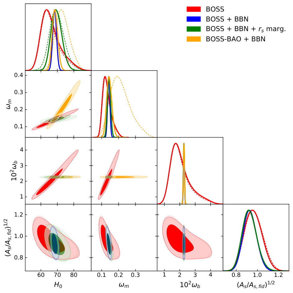
The results of this analysis are shown in Fig. 7, with posteriors given in Table 4. For the BOSS + Pantheon analyses, our results may be compared to (Philcox et al. 2020), which found ; here we find , with the slight broadening linked to the removal of broad and priors. For the BOSS + BBN analysis, which does depend on the sound horizon, the analogue is (Ivanov et al. 2020); this analysis obtained , similar to the results found herein. Finally, the BOSS BAO-only analysis may be compared to Fig. 2 of (Schöneberg et al. 2019). Of greatest interest are the constraints including both BBN and -marginalisation, i.e. those utilising the new methods developed in this work. As shown in the figure, the constraints including both -marginalisation and priors on are narrower than those obtained from the BOSS data alone, and the distribution is significantly closer to Gaussian. In both cases, we exclude sound-horizon information: first, explicitly, and second, by removal of the BBN prior. The addition of marginalisation and BBN information shrinks the posterior by () relative to the BOSS-only information (), or if Pantheon priors on are included ( for ‘FS+BBN+ marg.+Pantheon’ compared to ‘FS+Pantheon’). Without Pantheon priors, the marginalised full shape analysis is comparable to the BAO-only analysis. However, inclusion of prior information on from Pantheon leads to improved calibration of the sound-horizon feature, giving a tight constraint with from BAO alone, only somewhat wider than the FS + BBN results.
Additionally, we find a rise in the central value by and when BBN information is added in the analysis with and without priors on respectively. However, this is not unexpected given that new BBN data is added and the error bars change significantly, and so (as also suggested by a simple estimate1212 12 Following the prescription from Ref. Gratton and Challinor 2020 we estimate the significance of these shifts at and respectively. For this estimate we have taken half the posterior width as our estimate of the constraint on .) we do not affix any significance to this change; furthermore it is consistent with the BAO-only dataset. Notably, the increase in precision from adding BBN information (and marginalising over ) is less than would be expected from rescaling the Euclid results of §III to the BOSS effective volume. This can be understood by noting that the BBN prior on has the same fractional width in both scenarios. Given the smaller survey volume of BOSS, the BAO information is expected to have a greater impact, thus the equality constraints are fractionally weaker.
In the previous sections, we have demonstrated that constraints obtained using -marginalisation are sound-horizon independent for a Euclid-like survey, even when a BBN prior is applied. For BOSS, the same conclusion should naturally hold, since its volume (and thus the precision with which the equality and sound-horizon features can be measured) is much smaller. Our constraints, therefore, represent the tightest sound-horizon-independent bounds on from current galaxy surveys; including both BBN and Pantheon data, this has the value , fully consistent with the BAO-only constraints of (with the prior set by BBN and Pantheon). Whilst this result is not yet able to shed light on the so-called Hubble tension, it is a significant sharpening of previous constraints, and, as we have shown, such constraints are expected to tighten significantly with future data.
| BOSS | BOSS + Pantheon | |
|---|---|---|
| FS | ||
| FS + BBN | ||
| FS + BBN + marg. | ||
| BAO + BBN |
VI Conclusion
Obtaining accurate measurements of the Hubble parameter is a key goal for current and future galaxy surveys. In this work, we have demonstrated that a full shape (FS) analysis of forthcoming Euclid spectroscopic data has access to two powerful and physically independent probes of . When the analysis is performed with priors on the baryon density from BBN, the physical size of the sound horizon, , is calibrated and this information dominates the constraint. Without prior information on the constraints are instead dominated by the matter-radiation equality scale, , which is sensitive to higher-redshift physics. Here we have shown that, using a heuristic procedure to marginalise over the size of the sound horizon, we are able to avoid -based information entering our analysis even when including a prior on . This procedure leads to equality-based constraints on that are competitive with those derived from -based probes. Testing our method with an MCMC analysis of a mock Euclid likelihood, we forecast with this new method compared to from BAO information and for a full shape analysis without any external baryon information (in the manner suggested in previous works).
As discussed for example in Ref. Ross et al. 2012, systematic uncertainties on large scales arising for example from a spatially varying targeting efficiency on the sky (caused by various observational challenges such as atmospheric transparency, sky brightness or foreground contaminants) remain a major challenge for LSS surveys. It has been shown that while BAO observations are relatively insensitive to these systematics the broadband power spectrum can be significantly affected by spurious residuals, especially on large scales Ross et al. 2012. To perform a measurement as proposed in this work with future surveys it will be essential to demonstrate carefully that all relevant observational systematic effects are under control. Various mitigation strategies have been proposed for this purpose (see e.g. Ref. Weaverdyck and Huterer 2021). We defer a detailed investigation of systematic challenges to our method (and their mitigation) to future work.
In §III we have demonstrated that, when analyzing a mock dataset generated with a CDM cosmology, different analysis methods (FS, FS+BBN, FS+BBN+ marg. and BAO+BBN) yield consistent constraints on , as expected. When the data is instead generated from an EDE model, but analysed assuming CDM, we find measurable tensions between the constraints inferred from FS+BBN+ marg. and BAO+BBN analyses (see §IV). This occurs since a period of early dark energy domination affects the sound horizon and equality scales differently.
For the Planck+SH0ES best-fit model of (Smith et al. 2020), the shift in falls just short of being detected at ; however, if we instead use that of the latest ACT analyses (Hill et al. 2021), the shift increases to , due to the much larger EDE fraction. The results found herein demonstrate that our method can be used as a powerful null test for models of post-CDM physics. Since many approaches claiming to resolve the so-called Hubble tension modify the physical size of the sound horizon at the end to the baryon drag epoch, it is generically expected that such models would affect the sound horizon and the equality scale differently, thus leading to an inconsistency of the two measurements.
As mentioned previously, a multitude of different models have been proposed to resolve the so-called tension. Whilst the most stringent constraints on each of these models are certainly derived from a dedicated analysis, the effort necessary to probe (and wherever possible rule out) a large number of models as well as mechanisms that have not yet been proposed, makes it useful to generically test all -modifying models. With future surveys this approach will allow one to gauge how promising such modifications are as resolutions to the Hubble tension. A fully parametric model to fit the full shape power spectrum (as in Ref. Brieden et al. 2021) could provide a similar generic probe. However, there are in principle many ways to devise such a parametrisation, and hence we here chose a physically motivated approach that explicitly aims to decouple the two relevant sources of information contained within the power spectrum. It will be exciting to see the results of such studies applied to future data.
Acknowledgements.
We thank Graeme Addison, Eric Baxter, Florian Beutler, Simone Ferraro, Hector Gil-Marin, Colin Hill, Misha Ivanov, Adam Riess, Tristan Smith and Zvonimir Vlah for useful discussion and comments. We are additionally grateful to the anonymous referee for insightful comments. GSF acknowledges support through the Isaac Newton Studentship and the Helen Stone Scholarship at the University of Cambridge. OHEP acknowledges funding from the WFIRST program through NNG26PJ30C and NNN12AA01C and thanks the Simons Foundation for additional support. The authors are pleased to acknowledge that the work reported in this paper was substantially performed using the Helios cluster at the Institute for Advanced Study. Additional computations were performed using the Princeton Research Computing resources at Princeton University which is a consortium of groups led by the Princeton Institute for Computational Science and Engineering (PICSciE) and the Office of Information Technology’s Research Computing Division.Appendix A Broadband suppression
As mentioned in §II, the BAO feature is not the only source of information about (and thus ). Additionally, the sound horizon at photon-baryon decoupling also affects the scale on which baryonic effects suppress structure formation. This effect is typically relevant on scales similar to the BAO scale. Here we approximately marginalise over a shift in the baryon suppression scale by modifying the data covariance as described in §II. We conservatively assume that any rescaling of the baryon suppression scale is uncorrelated with other variations in the nonlinear power spectrum.
The results of analysing the mock Euclid data using the modified covariance matrix are shown in Fig. 8. We observe almost no difference between constraints derived with and without the broadband -marginalisation. In §III, we demonstrated that our constraints were independent of the sound horizon scale, even when neglecting the impact of on the broadband power spectrum; in concert with the above, this indicates that the effect of broadband -marginalisation for our Euclid analysis is negligible. We also verified this using a Fisher forecast run with an analytical Eisenstein-Hu Eisenstein and Hu 1998 transfer function in which we explicitly include marginalisation over the parameter which rescales the suppression scale as introduced in §II. We find no appreciable impact on cosmological parameter constraints. This analysis also indicates that changes in the baryon suppression scale are strongly degenerate with various bias and counterterm parameters. Both tests are sensitive only to the linear-order changes in the power spectrum induced by baryon suppression. However, we find that the higher-order derivatives of the power spectrum with respect to are negligible compared to the first, and hence we do not believe higher-order effects to be important.
Appendix B Constraints on from power spectra without the BAO feature
In Fig. 9 we show a comparison of parameter constraints from our FS forecasts to those obtained from a ‘no-wiggle’ power spectrum (including a BBN derived prior on in all cases). Such a ‘no-wiggle’ dataset is generated by setting the wiggly part of the power spectrum, (obtained as described in §II), to zero within CLASS-PT. We observe that while the constraint from the ‘no-wiggle’ analysis is significantly wider than the one from the ‘FS+BBN’ analysis, it matches that of the ‘FS+BBN+ marg.’ analysis well ( compared to respectively). This shows that meaningful constraints on can be derived from the broadband alone. However, constraints on a variety of other parameters, including for example , differ between the ‘no-wiggle’ and the -marginalised analyses. This indicates that, as discussed in the body of this work, there is residual, non--related, information contained in the ‘wiggly’ part of the power spectrum even when rescaled, such as the information on the baryon to dark matter density ratio encoded in the BAO peak heights. The good agreement between constraints is likely explained by a tradeoff between this additional information and the additional uncertainty in the broadband shape introduced by adding and shifting the ‘wiggly’ component.
Appendix C Analysis with varying and redshift selections
Here we consider different subsets of our data to explore the origin of the information content in our analysis. This is performed using Fisher forecasts for a Euclid-like survey, which were shown to be in excellent agreement with the MCMC analysis in § III.3.
First, we consider a range of different scale cuts, setting the maximum wavenumber in the analysis to , or (the latter being the default value in the above analysis). As mentioned in §III.1, our covariance matrix accounts for theoretical errors due to higher order loop corrections (see § III and Ref. Chudaykin and Ivanov 2019). This leads to the errors beyond increasing dramatically and the data becoming relatively uninformative on small scales even for the lowest redshift bins where shot noise is subdominant until (see Table 1). We thus expect only minor differences between and , matching the Fisher forecast results of Fig. 10. The figure also shows that, when -marginalisation is included, constraints are degraded for all three choices of , by a factor of 1.5, 2.0 and 1.7 for , , and respectively (cf. Table 5). Whilst there is little sound horizon information contained below , allowing the BAO scale to shift freely also degrades -derived constraints on . This occurs because the first BAO peak partially overlaps with the turnover scale of the power spectrum and -marginalisation therefore decreases the precision with which can be determined from the power spectrum.
Our -marginalised constraints are improved by a factor of 2.2 when increasing our from to ; the unmarginalised constraints are improved by a factor of 3. While this is in contrast to our previous work Philcox et al. 2020 where we saw little improvement in the equality derived constraints when increasing beyond , it is expected since with our new method we are able to use some of the information contained in the BAO feature as discussed previously while explicitly removing the information on the sound horizon scale. One also expects the more dramatic improvement in the unmarginalised constraints since essentially all the BAO information falls within this range.
Secondly, we divide our data into low-, medium- and high-redshift bins. As discussed above, the fiducial analysis uses eight redshift bins evenly spaced between and . Our low-redshift dataset contains the lowest two redshift bins ( and ), the medium-redshift sample consists of the redshift bins with mean redshifts and , while the remaining four redshift bins (, , and ) make up the high-redshift subset. One can see in Fig. 11 that without -marginalisation, we expect similar constraints from each of the three subsets (see Table 5 for forecast uncertainties). When including our sound horizon marginalisation procedure, the high- and medium-redshift constraints are more significantly degraded. Our analysis thus increases the relative weight of the low-redshift data.
| FS + BBN | FS + BBN + marg. | |
|---|---|---|
| selection | FS + BBN | FS + BBN + marg. |
|---|---|---|


References
- Planck Collaboration et al. (2020) Planck Collaboration, N. Aghanim, Y. Akrami, M. Ashdown, J. Aumont, C. Baccigalupi, M. Ballardini, A. J. Banday, R. B. Barreiro, N. Bartolo, S. Basak, R. Battye, K. Benabed, J. P. Bernard, M. Bersanelli, P. Bielewicz, J. J. Bock, J. R. Bond, J. Borrill, F. R. Bouchet, F. Boulanger, M. Bucher, C. Burigana, R. C. Butler, E. Calabrese, J. F. Cardoso, J. Carron, A. Challinor, H. C. Chiang, J. Chluba, L. P. L. Colombo, C. Combet, D. Contreras, B. P. Crill, F. Cuttaia, P. de Bernardis, G. de Zotti, J. Delabrouille, J. M. Delouis, E. Di Valentino, J. M. Diego, O. Doré, M. Douspis, A. Ducout, X. Dupac, S. Dusini, G. Efstathiou, F. Elsner, T. A. Enßlin, H. K. Eriksen, Y. Fantaye, M. Farhang, J. Fergusson, R. Fernandez-Cobos, F. Finelli, F. Forastieri, M. Frailis, A. A. Fraisse, E. Franceschi, A. Frolov, S. Galeotta, S. Galli, K. Ganga, R. T. Génova-Santos, M. Gerbino, T. Ghosh, J. González-Nuevo, K. M. Górski, S. Gratton, A. Gruppuso, J. E. Gudmundsson, J. Hamann, W. Handley, F. K. Hansen, D. Herranz, S. R. Hildebrandt, E. Hivon, Z. Huang, A. H. Jaffe, W. C. Jones, A. Karakci, E. Keihänen, R. Keskitalo, K. Kiiveri, J. Kim, T. S. Kisner, L. Knox, N. Krachmalnicoff, M. Kunz, H. Kurki-Suonio, G. Lagache, J. M. Lamarre, A. Lasenby, M. Lattanzi, C. R. Lawrence, M. Le Jeune, P. Lemos, J. Lesgourgues, F. Levrier, A. Lewis, M. Liguori, P. B. Lilje, M. Lilley, V. Lindholm, M. López-Caniego, P. M. Lubin, Y. Z. Ma, J. F. Macías-Pérez, G. Maggio, D. Maino, N. Mandolesi, A. Mangilli, A. Marcos-Caballero, M. Maris, P. G. Martin, M. Martinelli, E. Martínez-González, S. Matarrese, N. Mauri, J. D. McEwen, P. R. Meinhold, A. Melchiorri, A. Mennella, M. Migliaccio, M. Millea, S. Mitra, M. A. Miville-Deschênes, D. Molinari, L. Montier, G. Morgante, A. Moss, P. Natoli, H. U. Nørgaard-Nielsen, L. Pagano, D. Paoletti, B. Partridge, G. Patanchon, H. V. Peiris, F. Perrotta, V. Pettorino, F. Piacentini, L. Polastri, G. Polenta, J. L. Puget, J. P. Rachen, M. Reinecke, M. Remazeilles, A. Renzi, G. Rocha, C. Rosset, G. Roudier, J. A. Rubiño-Martín, B. Ruiz-Granados, L. Salvati, M. Sandri, M. Savelainen, D. Scott, E. P. S. Shellard, C. Sirignano, G. Sirri, L. D. Spencer, R. Sunyaev, A. S. Suur-Uski, J. A. Tauber, D. Tavagnacco, M. Tenti, L. Toffolatti, M. Tomasi, T. Trombetti, L. Valenziano, J. Valiviita, B. Van Tent, L. Vibert, P. Vielva, F. Villa, N. Vittorio, B. D. Wand elt, I. K. Wehus, M. White, S. D. M. White, A. Zacchei, and A. Zonca, Planck 2018 results. VI. Cosmological parameters, A&A 641, A6 (2020), arXiv:1807.06209 [astro-ph.CO] .
- Riess et al. (2019) A. G. Riess, S. Casertano, W. Yuan, L. M. Macri, and D. Scolnic, Large Magellanic Cloud Cepheid Standards Provide a 1% Foundation for the Determination of the Hubble Constant and Stronger Evidence for Physics beyond CDM, ApJ 876, 85 (2019), arXiv:1903.07603 [astro-ph.CO] .
- Schombert et al. (2020) J. Schombert, S. McGaugh, and F. Lelli, Using the Baryonic Tully-Fisher Relation to Measure Ho, AJ 160, 71 (2020), arXiv:2006.08615 [astro-ph.CO] .
- Riess et al. (2021a) A. G. Riess, S. Casertano, W. Yuan, J. B. Bowers, L. Macri, J. C. Zinn, and D. Scolnic, Cosmic distances calibrated to 1% precision with gaia edr3 parallaxes and hubble space telescope photometry of 75 milky way cepheids confirm tension with CDM, The Astrophysical Journal 908, L6 (2021a).
- Riess et al. (2021b) A. G. Riess, W. Yuan, L. M. Macri, D. Scolnic, D. Brout, S. Casertano, D. O. Jones, Y. Murakami, L. Breuval, T. G. Brink, A. V. Filippenko, S. Hoffmann, S. W. Jha, W. D. Kenworthy, J. Mackenty, B. E. Stahl, and W. Zheng, A comprehensive measurement of the local value of the hubble constant with 1 km/s/mpc uncertainty from the hubble space telescope and the SH0ES team, (2021b), arXiv:2112.04510 [astro-ph.CO] .
- Alam et al. (2017) S. Alam, M. Ata, S. Bailey, F. Beutler, D. Bizyaev, J. A. Blazek, A. S. Bolton, J. R. Brownstein, A. Burden, C.-H. Chuang, J. Comparat, A. J. Cuesta, K. S. Dawson, D. J. Eisenstein, S. Escoffier, H. Gil-Marín, J. N. Grieb, N. Hand, S. Ho, K. Kinemuchi, D. Kirkby, F. Kitaura, E. Malanushenko, V. Malanushenko, C. Maraston, C. K. McBride, R. C. Nichol, M. D. Olmstead, D. Oravetz, N. Padmanabhan, N. Palanque-Delabrouille, K. Pan, M. Pellejero-Ibanez, W. J. Percival, P. Petitjean, F. Prada, A. M. Price-Whelan, B. A. Reid, S. A. Rodríguez-Torres, N. A. Roe, A. J. Ross, N. P. Ross, G. Rossi, J. A. Rubiño-Martín, S. Saito, S. Salazar-Albornoz, L. Samushia, A. G. Sánchez, S. Satpathy, D. J. Schlegel, D. P. Schneider, C. G. Scóccola, H.-J. Seo, E. S. Sheldon, A. Simmons, A. Slosar, M. A. Strauss, M. E. C. Swanson, D. Thomas, J. L. Tinker, R. Tojeiro, M. V. Magaña, J. A. Vazquez, L. Verde, D. A. Wake, Y. Wang, D. H. Weinberg, M. White, W. M. Wood-Vasey, C. Yèche, I. Zehavi, Z. Zhai, and G.-B. Zhao, The clustering of galaxies in the completed SDSS-III Baryon Oscillation Spectroscopic Survey: cosmological analysis of the DR12 galaxy sample, MNRAS 470, 2617 (2017), arXiv:1607.03155 [astro-ph.CO] .
- Cuceu et al. (2019) A. Cuceu, J. Farr, P. Lemos, and A. Font-Ribera, Baryon Acoustic Oscillations and the Hubble constant: past, present and future, JCAP 2019, 044 (2019), arXiv:1906.11628 [astro-ph.CO] .
- Abbott et al. (2018) T. M. C. Abbott, F. B. Abdalla, J. Annis, K. Bechtol, J. Blazek, B. A. Benson, R. A. Bernstein, G. M. Bernstein, E. Bertin, D. Brooks, D. L. Burke, A. Carnero Rosell, M. Carrasco Kind, J. Carretero, F. J. Castander, C. L. Chang, T. M. Crawford, C. E. Cunha, C. B. D’Andrea, L. N. da Costa, C. Davis, J. DeRose, S. Desai, H. T. Diehl, J. P. Dietrich, P. Doel, A. Drlica-Wagner, A. E. Evrard, E. Fernand ez, B. Flaugher, P. Fosalba, J. Frieman, J. García-Bellido, E. Gaztanaga, D. W. Gerdes, T. Giannantonio, D. Gruen, R. A. Gruendl, J. Gschwend, G. Gutierrez, W. G. Hartley, J. W. Henning, K. Honscheid, B. Hoyle, D. Huterer, B. Jain, D. J. James, M. Jarvis, T. Jeltema, M. D. Johnson, M. W. G. Johnson, E. Krause, K. Kuehn, S. Kuhlmann, N. Kuropatkin, O. Lahav, A. R. Liddle, M. Lima, H. Lin, N. MacCrann, M. A. G. Maia, A. Manzotti, M. March, J. L. Marshall, R. Miquel, J. J. Mohr, T. Natoli, P. Nugent, R. L. C. Ogando, Y. Park, A. A. Plazas, C. L. Reichardt, K. Reil, A. Roodman, A. J. Ross, E. Rozo, E. S. Rykoff, E. Sanchez, V. Scarpine, M. Schubnell, D. Scolnic, I. Sevilla-Noarbe, E. Sheldon, M. Smith, R. C. Smith, M. Soares-Santos, F. Sobreira, E. Suchyta, G. Tarle, D. Thomas, M. A. Troxel, A. R. Walker, R. H. Wechsler, J. Weller, W. Wester, W. L. K. Wu, J. Zuntz, Dark Energy Survey Collaboration, and South Pole Telescope Collaboration, Dark Energy Survey Year 1 Results: A Precise H0 Estimate from DES Y1, BAO, and D/H Data, MNRAS 480, 3879 (2018), arXiv:1711.00403 [astro-ph.CO] .
- Aylor et al. (2019) K. Aylor, M. Joy, L. Knox, M. Millea, S. Raghunathan, and W. L. Kimmy Wu, Sounds Discordant: Classical Distance Ladder and CDM-based Determinations of the Cosmological Sound Horizon, ApJ 874, 4 (2019), arXiv:1811.00537 [astro-ph.CO] .
- Schöneberg et al. (2019) N. Schöneberg, J. Lesgourgues, and D. C. Hooper, The BAO+BBN take on the Hubble tension, JCAP 2019, 029 (2019), arXiv:1907.11594 [astro-ph.CO] .
- Addison et al. (2018) G. E. Addison, D. J. Watts, C. L. Bennett, M. Halpern, G. Hinshaw, and J. L. Weiland, Elucidating CDM: Impact of Baryon Acoustic Oscillation Measurements on the Hubble Constant Discrepancy, ApJ 853, 119 (2018), arXiv:1707.06547 [astro-ph.CO] .
- Colas et al. (2020) T. Colas, G. d’Amico, L. Senatore, P. Zhang, and F. Beutler, Efficient cosmological analysis of the SDSS/BOSS data from the Effective Field Theory of Large-Scale Structure, JCAP 2020, 001 (2020), arXiv:1909.07951 [astro-ph.CO] .
- eBOSS Collaboration et al. (2020) eBOSS Collaboration, S. Alam, M. Aubert, S. Avila, C. Balland, J. E. Bautista, M. A. Bershady, D. Bizyaev, M. R. Blanton, A. S. Bolton, J. Bovy, J. Brinkmann, J. R. Brownstein, E. Burtin, S. Chabanier, M. J. Chapman, P. D. Choi, C.-H. Chuang, J. Comparat, A. Cuceu, K. S. Dawson, A. de la Macorra, S. de la Torre, A. de Mattia, V. de Sainte Agathe, H. du Mas des Bourboux, S. Escoffier, T. Etourneau, J. Farr, A. Font-Ribera, P. M. Frinchaboy, S. Fromenteau, H. Gil-Marín, A. X. Gonzalez-Morales, V. Gonzalez-Perez, K. Grabowski, J. Guy, A. J. Hawken, J. Hou, H. Kong, M. Klaene, J.-P. Kneib, J.-M. Le Goff, S. Lin, D. Long, B. W. Lyke, M.-C. Cousinou, P. Martini, K. Masters, F. G. Mohammad, J. Moon, E.-M. Mueller, A. Munõz-Gutieŕrez, A. D. Myers, S. Nadathur, R. Neveux, J. A. Newman, P. Noterdaeme, A. Oravetz, D. Oravetz, N. Palanque-Delabrouille, K. Pan, I. Parker, James, R. Paviot, W. J. Percival, I. Peŕez-Rafols, P. Petitjean, M. M. Pieri, A. Prakash, A. Raichoor, C. Ravoux, M. Rezaie, J. Rich, A. J. Ross, G. Rossi, R. Ruggeri, V. Ruhlmann-Kleider, A. G. Sańchez, F. J. Sańchez, J. R. Sańchez-Gallego, C. Sayres, D. P. Schneider, H.-J. Seo, A. Shafieloo, A. Slosar, A. Smith, J. Stermer, A. Tamone, J. L. Tinker, R. Tojeiro, M. Vargas-Magaña, A. Variu, Y. Wang, B. A. Weaver, A.-M. Weijmans, C. Yeche, P. Zarrouk, C. Zhao, G.-B. Zhao, and Z. Zheng, The Completed SDSS-IV extended Baryon Oscillation Spectroscopic Survey: Cosmological Implications from two Decades of Spectroscopic Surveys at the Apache Point observatory, arXiv e-prints , arXiv:2007.08991 (2020), arXiv:2007.08991 [astro-ph.CO] .
- d’Amico et al. (2020) G. d’Amico, J. Gleyzes, N. Kokron, K. Markovic, L. Senatore, P. Zhang, F. Beutler, and H. Gil-Marín, The cosmological analysis of the SDSS/BOSS data from the Effective Field Theory of Large-Scale Structure, JCAP 2020, 005 (2020), arXiv:1909.05271 [astro-ph.CO] .
- Philcox et al. (2020) O. H. E. Philcox, M. M. Ivanov, M. Simonović, and M. Zaldarriaga, Combining full-shape and BAO analyses of galaxy power spectra: a 1.6% CMB-independent constraint on H0, JCAP 2020, 032 (2020), arXiv:2002.04035 [astro-ph.CO] .
- Zhang et al. (2021) P. Zhang, G. D’Amico, L. Senatore, C. Zhao, and Y. Cai, BOSS Correlation Function Analysis from the Effective Field Theory of Large-Scale Structure, arXiv e-prints , arXiv:2110.07539 (2021), arXiv:2110.07539 [astro-ph.CO] .
- Chen et al. (2021) S.-F. Chen, Z. Vlah, and M. White, A new analysis of the BOSS survey, including full-shape information and post-reconstruction BAO, arXiv e-prints , arXiv:2110.05530 (2021), arXiv:2110.05530 [astro-ph.CO] .
- Freedman et al. (2019) W. L. Freedman, B. F. Madore, D. Hatt, T. J. Hoyt, I. S. Jang, R. L. Beaton, C. R. Burns, M. G. Lee, A. J. Monson, J. R. Neeley, M. M. Phillips, J. A. Rich, and M. Seibert, The Carnegie-Chicago Hubble Program. VIII. An Independent Determination of the Hubble Constant Based on the Tip of the Red Giant Branch, ApJ 882, 34 (2019), arXiv:1907.05922 [astro-ph.CO] .
- Birrer et al. (2020) S. Birrer, A. J. Shajib, A. Galan, M. Millon, T. Treu, A. Agnello, M. Auger, G. C. F. Chen, L. Christensen, T. Collett, F. Courbin, C. D. Fassnacht, L. V. E. Koopmans, P. J. Marshall, J. W. Park, C. E. Rusu, D. Sluse, C. Spiniello, S. H. Suyu, S. Wagner-Carena, K. C. Wong, M. Barnabè, A. S. Bolton, O. Czoske, X. Ding, J. A. Frieman, and L. Van de Vyvere, TDCOSMO IV: Hierarchical time-delay cosmography – joint inference of the Hubble constant and galaxy density profiles, arXiv e-prints , arXiv:2007.02941 (2020), arXiv:2007.02941 [astro-ph.CO] .
- Knox and Millea (2020) L. Knox and M. Millea, Hubble constant hunter’s guide, Phys. Rev. D 101, 043533 (2020).
- Di Valentino et al. (2021) E. Di Valentino, O. Mena, S. Pan, L. Visinelli, W. Yang, A. Melchiorri, D. F. Mota, A. G. Riess, and J. Silk, In the realm of the hubble tension—a review of solutions, Classical and Quantum Gravity 38, 153001 (2021).
- Hill et al. (2020) J. C. Hill, E. McDonough, M. W. Toomey, and S. Alexander, Early dark energy does not restore cosmological concordance, Phys. Rev. D 102, 043507 (2020), arXiv:2003.07355 [astro-ph.CO] .
- Hill et al. (2021) J. C. Hill, E. Calabrese, S. Aiola, N. Battaglia, B. Bolliet, S. K. Choi, M. J. Devlin, A. J. Duivenvoorden, J. Dunkley, S. Ferraro, P. A. Gallardo, V. Gluscevic, M. Hasselfield, M. Hilton, A. D. Hincks, R. Hlozek, B. J. Koopman, A. Kosowsky, A. La Posta, T. Louis, M. S. Madhavacheril, J. McMahon, K. Moodley, S. Naess, U. Natale, F. Nati, L. Newburgh, M. D. Niemack, B. Partridge, F. J. Qu, M. Salatino, A. Schillaci, N. Sehgal, B. D. Sherwin, C. Sifon, D. N. Spergel, S. T. Staggs, E. R. Storer, A. van Engelen, E. M. Vavagiakis, E. J. Wollack, and Z. Xu, The Atacama Cosmology Telescope: Constraints on Pre-Recombination Early Dark Energy, arXiv e-prints , arXiv:2109.04451 (2021), arXiv:2109.04451 [astro-ph.CO] .
- Baxter and Sherwin (2020) E. J. Baxter and B. D. Sherwin, Determining the hubble constant without the sound horizon scale: measurements from cmb lensing, Monthly Notices of the Royal Astronomical Society 501, 1823–1835 (2020).
- Philcox et al. (2020) O. H. E. Philcox, B. D. Sherwin, G. S. Farren, and E. J. Baxter, Determining the Hubble Constant without the Sound Horizon: Measurements from Galaxy Surveys, (2020), arXiv:2008.08084 .
- Eisenstein and Hu (1998) D. J. Eisenstein and W. Hu, Baryonic Features in the Matter Transfer Function, ApJ 496, 605 (1998), arXiv:astro-ph/9709112 [astro-ph] .
- Chudaykin and Ivanov (2019) A. Chudaykin and M. M. Ivanov, Measuring neutrino masses with large-scale structure: Euclid forecast with controlled theoretical error, JCAP 2019, 034 (2019), arXiv:1907.06666 [astro-ph.CO] .
- Poulin et al. (2019) V. Poulin, T. L. Smith, T. Karwal, and M. Kamionkowski, Early dark energy can resolve the hubble tension, Physical Review Letters 122, 10.1103/physrevlett.122.221301 (2019).
- Smith et al. (2020) T. L. Smith, V. Poulin, and M. A. Amin, Oscillating scalar fields and the hubble tension: A resolution with novel signatures, Phys. Rev. D 101, 063523 (2020).
- Lin et al. (2019) M.-X. Lin, G. Benevento, W. Hu, and M. Raveri, Acoustic dark energy: Potential conversion of the hubble tension, Physical Review D 100, 10.1103/physrevd.100.063542 (2019).
- Lin et al. (2020) M.-X. Lin, W. Hu, and M. Raveri, Testing h0 in acoustic dark energy models with planck and act polarization data, Physical Review D 102, 10.1103/physrevd.102.123523 (2020).
- Sakstein and Trodden (2020) J. Sakstein and M. Trodden, Early dark energy from massive neutrinos as a natural resolution of the hubble tension, Physical Review Letters 124, 10.1103/physrevlett.124.161301 (2020).
- Niedermann and Sloth (2021a) F. Niedermann and M. S. Sloth, New early dark energy, Phys. Rev. D 103, L041303 (2021a).
- Ivanov et al. (2020) M. M. Ivanov, E. McDonough, J. C. Hill, M. Simonović, M. W. Toomey, S. Alexander, and M. Zaldarriaga, Constraining early dark energy with large-scale structure, Phys. Rev. D 102, 103502 (2020).
- D’Amico et al. (2021) G. D’Amico, L. Senatore, P. Zhang, and H. Zheng, The hubble tension in light of the full-shape analysis of large-scale structure data, Journal of Cosmology and Astroparticle Physics 2021 (05), 072.
- Niedermann and Sloth (2021b) F. Niedermann and M. S. Sloth, New early dark energy is compatible with current lss data, Phys. Rev. D 103, 103537 (2021b).
- Smith et al. (2021) T. L. Smith, V. Poulin, J. L. Bernal, K. K. Boddy, M. Kamionkowski, and R. Murgia, Early dark energy is not excluded by current large-scale structure data, Phys. Rev. D 103, 123542 (2021).
- Ivanov and Sibiryakov (2018) M. M. Ivanov and S. Sibiryakov, Infrared resummation for biased tracers in redshift space, JCAP 2018, 053 (2018), arXiv:1804.05080 [astro-ph.CO] .
- Chudaykin et al. (2020) A. Chudaykin, M. M. Ivanov, O. H. E. Philcox, and M. Simonović, Nonlinear perturbation theory extension of the boltzmann code class, Phys. Rev. D 102, 063533 (2020).
- Chudaykin and Ivanov (2019) A. Chudaykin and M. M. Ivanov, Measuring neutrino masses with large-scale structure: Euclid forecast with controlled theoretical error, Journal of Cosmology and Astroparticle Physics arXiv:1907.06666 .
- Philcox et al. (2020) O. H. E. Philcox, M. M. Ivanov, M. Zaldarriaga, M. Simonović, and M. M. Schmittfull, Fewer Mocks and Less Noise: Reducing the Dimensionality of Cosmological Observables with Subspace Projections, in prep. (2020).
- Taylor and Kitching (2010) A. N. Taylor and T. D. Kitching, Analytic methods for cosmological likelihoods, MNRAS 408, 865 (2010), arXiv:1003.1136 [astro-ph.CO] .
- Ivanov et al. (2020) M. M. Ivanov, M. Simonović, and M. Zaldarriaga, Cosmological parameters from the BOSS galaxy power spectrum, JCAP 2020, 042 (2020), arXiv:1909.05277 [astro-ph.CO] .
- Ivanov (2021) M. M. Ivanov, Cosmological constraints from the power spectrum of eBOSS emission line galaxies, arXiv e-prints , arXiv:2106.12580 (2021), arXiv:2106.12580 [astro-ph.CO] .
- Baldauf et al. (2016) T. Baldauf, M. Mirbabayi, M. Simonović, and M. Zaldarriaga, LSS constraints with controlled theoretical uncertainties, arXiv e-prints , arXiv:1602.00674 (2016), arXiv:1602.00674 [astro-ph.CO] .
- Beutler et al. (2017) F. Beutler, H.-J. Seo, A. J. Ross, P. McDonald, S. Saito, A. S. Bolton, J. R. Brownstein, C.-H. Chuang, A. J. Cuesta, D. J. Eisenstein, A. Font-Ribera, J. N. Grieb, N. Hand, F.-S. Kitaura, C. Modi, R. C. Nichol, W. J. Percival, F. Prada, S. Rodriguez-Torres, N. A. Roe, N. P. Ross, S. Salazar-Albornoz, A. G. Sánchez, D. P. Schneider, A. Slosar, J. Tinker, R. Tojeiro, M. Vargas-Magaña, and J. A. Vazquez, The clustering of galaxies in the completed SDSS-III Baryon Oscillation Spectroscopic Survey: baryon acoustic oscillations in the Fourier space, MNRAS 464, 3409 (2017), arXiv:1607.03149 [astro-ph.CO] .
- Aubourg et al. (2015) É. Aubourg, S. Bailey, J. E. Bautista, F. Beutler, V. Bhardwaj, D. Bizyaev, M. Blanton, M. Blomqvist, A. S. Bolton, J. Bovy, H. Brewington, J. Brinkmann, J. R. Brownstein, A. Burden, N. G. Busca, W. Carithers, C.-H. Chuang, J. Comparat, R. A. C. Croft, A. J. Cuesta, K. S. Dawson, T. Delubac, D. J. Eisenstein, A. Font-Ribera, J. Ge, J. M. Le Goff, S. G. A. Gontcho, J. R. Gott, J. E. Gunn, H. Guo, J. Guy, J.-C. Hamilton, S. Ho, K. Honscheid, C. Howlett, D. Kirkby, F. S. Kitaura, J.-P. Kneib, K.-G. Lee, D. Long, R. H. Lupton, M. V. Magaña, V. Malanushenko, E. Malanushenko, M. Manera, C. Maraston, D. Margala, C. K. McBride, J. Miralda-Escudé, A. D. Myers, R. C. Nichol, P. Noterdaeme, S. E. Nuza, M. D. Olmstead, D. Oravetz, I. Pâris, N. Padmanabhan, N. Palanque-Delabrouille, K. Pan, M. Pellejero-Ibanez, W. J. Percival, P. Petitjean, M. M. Pieri, F. Prada, B. Reid, J. Rich, N. A. Roe, A. J. Ross, N. P. Ross, G. Rossi, J. A. Rubiño-Martín, A. G. Sánchez, L. Samushia, R. T. Génova-Santos, C. G. Scóccola, D. J. Schlegel, D. P. Schneider, H.-J. Seo, E. Sheldon, A. Simmons, R. A. Skibba, A. Slosar, M. A. Strauss, D. Thomas, J. L. Tinker, R. Tojeiro, J. A. Vazquez, M. Viel, D. A. Wake, B. A. Weaver, D. H. Weinberg, W. M. Wood-Vasey, C. Yèche, I. Zehavi, G.-B. Zhao, and BOSS Collaboration, Cosmological implications of baryon acoustic oscillation measurements, Phys. Rev. D 92, 123516 (2015), arXiv:1411.1074 [astro-ph.CO] .
- Karwal and Kamionkowski (2016) T. Karwal and M. Kamionkowski, Dark energy at early times, the Hubble parameter, and the string axiverse, Phys. Rev. D 94, 103523 (2016), arXiv:1608.01309 [astro-ph.CO] .
- Mörtsell and Dhawan (2018) E. Mörtsell and S. Dhawan, Does the Hubble constant tension call for new physics?, JCAP 2018, 025 (2018), arXiv:1801.07260 [astro-ph.CO] .
- Poulin et al. (2019) V. Poulin, T. L. Smith, T. Karwal, and M. Kamionkowski, Early Dark Energy can Resolve the Hubble Tension, Phys. Rev. Lett. 122, 221301 (2019), arXiv:1811.04083 [astro-ph.CO] .
- Riess (2019) A. G. Riess, The expansion of the Universe is faster than expected, Nature Reviews Physics 2, 10 (2019), arXiv:2001.03624 [astro-ph.CO] .
- de Mattia and Ruhlmann-Kleider (2019) A. de Mattia and V. Ruhlmann-Kleider, Integral constraints in spectroscopic surveys, JCAP 2019, 036 (2019), arXiv:1904.08851 [astro-ph.CO] .
- de Mattia et al. (2021) A. de Mattia, V. Ruhlmann-Kleider, A. Raichoor, A. J. Ross, A. Tamone, C. Zhao, S. Alam, S. Avila, E. Burtin, J. Bautista, F. Beutler, J. Brinkmann, J. R. Brownstein, M. J. Chapman, C.-H. Chuang, J. Comparat, H. du Mas des Bourboux, K. S. Dawson, A. de la Macorra, H. Gil-Marín, V. Gonzalez-Perez, C. Gorgoni, J. Hou, H. Kong, S. Lin, S. Nadathur, J. A. Newman, E.-M. Mueller, W. J. Percival, M. Rezaie, G. Rossi, D. P. Schneider, P. Tiwari, M. Vivek, Y. Wang, and G.-B. Zhao, The completed SDSS-IV extended Baryon Oscillation Spectroscopic Survey: measurement of the BAO and growth rate of structure of the emission line galaxy sample from the anisotropic power spectrum between redshift 0.6 and 1.1, MNRAS 501, 5616 (2021), arXiv:2007.09008 [astro-ph.CO] .
- Beutler and McDonald (2021) F. Beutler and P. McDonald, Unified galaxy power spectrum measurements from 6dFGS, BOSS, and eBOSS, arXiv e-prints , arXiv:2106.06324 (2021), arXiv:2106.06324 [astro-ph.CO] .
- Poulin et al. (2021) V. Poulin, T. L. Smith, and A. Bartlett, Dark energy at early times and act: a larger hubble constant without late-time priors, (2021), arXiv:2109.06229 [astro-ph.CO] .
- Baxter and Sherwin (2020) E. J. Baxter and B. D. Sherwin, Determining the Hubble Constant without the Sound Horizon Scale: Measurements from CMB Lensing, arXiv e-prints , arXiv:2007.04007 (2020), arXiv:2007.04007 [astro-ph.CO] .
- Scolnic et al. (2018) D. M. Scolnic, D. O. Jones, A. Rest, Y. C. Pan, R. Chornock, R. J. Foley, M. E. Huber, R. Kessler, G. Narayan, A. G. Riess, S. Rodney, E. Berger, D. J. Brout, P. J. Challis, M. Drout, D. Finkbeiner, R. Lunnan, R. P. Kirshner, N. E. Sand ers, E. Schlafly, S. Smartt, C. W. Stubbs, J. Tonry, W. M. Wood-Vasey, M. Foley, J. Hand, E. Johnson, W. S. Burgett, K. C. Chambers, P. W. Draper, K. W. Hodapp, N. Kaiser, R. P. Kudritzki, E. A. Magnier, N. Metcalfe, F. Bresolin, E. Gall, R. Kotak, M. McCrum, and K. W. Smith, The Complete Light-curve Sample of Spectroscopically Confirmed SNe Ia from Pan-STARRS1 and Cosmological Constraints from the Combined Pantheon Sample, ApJ 859, 101 (2018), arXiv:1710.00845 [astro-ph.CO] .
- Gratton and Challinor (2020) S. Gratton and A. Challinor, Understanding parameter differences between analyses employing nested data subsets, Monthly Notices of the Royal Astronomical Society 499, 3410 (2020), https://academic.oup.com/mnras/article-pdf/499/3/3410/34052415/staa2996.pdf .
- Ross et al. (2012) A. J. Ross, W. J. Percival, A. G. Sánchez, L. Samushia, S. Ho, E. Kazin, M. Manera, B. Reid, M. White, R. Tojeiro, C. K. McBride, X. Xu, D. A. Wake, M. A. Strauss, F. Montesano, M. E. C. Swanson, S. Bailey, A. S. Bolton, A. M. Dorta, D. J. Eisenstein, H. Guo, J.-C. Hamilton, R. C. Nichol, N. Padmanabhan, F. Prada, D. J. Schlegel, M. V. Magaña, I. Zehavi, M. Blanton, D. Bizyaev, H. Brewington, A. J. Cuesta, E. Malanushenko, V. Malanushenko, D. Oravetz, J. Parejko, K. Pan, D. P. Schneider, A. Shelden, A. Simmons, S. Snedden, and G.-b. Zhao, The clustering of galaxies in the SDSS-III Baryon Oscillation Spectroscopic Survey: analysis of potential systematics, Monthly Notices of the Royal Astronomical Society 424, 564 (2012), https://academic.oup.com/mnras/article-pdf/424/1/564/3289224/mnras0424-0564.pdf .
- Weaverdyck and Huterer (2021) N. Weaverdyck and D. Huterer, Mitigating contamination in lss surveys: a comparison of methods, Monthly Notices of the Royal Astronomical Society 503, 5061–5084 (2021).
- Brieden et al. (2021) S. Brieden, H. Gil-Marín, and L. Verde, ShapeFit: Extracting the power spectrum shape information in galaxy surveys beyond BAO and RSD, arXiv e-prints , arXiv:2106.07641 (2021), arXiv:2106.07641 [astro-ph.CO] .