Study of the hidden charm interactions in chiral effective field theory
Abstract
We study the chiral interactions of the hidden charm system within chiral effective field theory. Chiral Lagrangians are constructed by incorporating the chiral symmetry, heavy quark symmetry as well as proper charge conjugation properties of the heavy mesons. The interacting potentials of the -wave are calculated up to second chiral order at 1-loop level, where complete two-pion exchange interactions are included. We further investigate the behaviors of the potentials in coordinate space, as well as their bound state properties. Our studies indicate that there exists a interacting strength ordering among considered four channels: where str. stands for the strength of the interaction. Moreover, we find that can be treated as a good candidate of molecular state. There also tends to form and molecular states and we expect the experiments to search for the predicted multi-structures around the mass region.
I introduction
In past two decades, abundant exotic hadrons have been discovered by upgraded -charm and factories such as the BESIII, LHCb, Belle, and etc. Till now, there has been various forms of exotic quark matters raising in hadron spectroscopy: pentaquarks ( and states), fully charmed tetraquark candidates (recently discovered ), hidden charm tetraquark candidates (some states), and etc. For example, was discovered by the LHCb recently Aaij:2020fnh, which appears to be a non-trivial structure in the di- invariant mass spectrum. Subsequently, the LHCb Collaboration also reported two structures and in the decay Aaij:2020ypa, which are supposed to have four different flavors: . In very recent, the LHCb observed a double charmed structure LHCb:2021vvq which is extremely close to threshold (the mass difference is keV). has a minimal content. Therefore, one can see it may still be an ongoing progress that other forms of multiquark structures are prepared to be uncovered. The rapidly growing numbers of exotic hadrons Urgently demand us to extend our knowledge about non-perturbative QCD.
Although studies of exotic hadrons on the experiment side are in advance, their natures and inner structures are still unclear. Theorists try to understand them with all kinds of methods and models, see Refs. Chen:2016qju; Esposito:2016noz; Lebed:2016hpi; Guo:2017jvc; Brambilla:2019esw; Liu:2019zoy for reviews of theoretical as well as experimental status.
For example, people still can not truly understand the nature of first observed state, (aka ). was discovered by the Belle collaboration in Choi:2003ue. It may be regarded as a charmonium with , but its mass would be much lower than quark model estimate (e.g. the GI model calculation in Ref. Godfrey:1985xj). Furthermore, it also has a large decay ratio in the isospin violation process . It is noteworthy that is almost located at threshold, so it is believed that the interaction between pair is strongly responsible for the formation of .
Besides , there also exists many other states that may strongly relate to open-charm thresholds. The charged charmonium-like state was observed in the process Ablikim:2013mio; Liu:2013dau, with the mass slightly above threshold it may originate from interaction. Other states such as Ablikim:2013wzq, Abe:2004zs and Aaltonen:2009tz are close to respective and thresholds too. There also exists some higher states that are close to excited open-charm thresholds: Choi:2007wga with , recently discovered Jia:2019gfe (and Jia:2020epr) with , and etc. Taking into account the interactions of these open-charm meson pairs, people have tried to explain these states with phenomenological models, such as one boson exchange model Chen:2016qju; Wang:2021aql.
Therefore, for understanding states mentioned above, it is crucial to elaborately investigate corresponding charmed- anticharmed meson interactions within a proper theoretical framework. Chiral effective field theory (ChEFT) is just the powerful formalism that satisfies the needs. Other than phenomenological models, in ChEFT, the interactions between hadrons are strictly and systematically calculated up to a given order, while all contributions such as multi pion exchange are contained in complete. Especially, in our case (i.e. heavy-heavy system) Weinberg’s formalism is adopted Weinberg:1990rz; Weinberg:1991um, which has been widely used to investigate the nucleon-nucleon interaction Ordonez:1992xp; Ordonez:1995rz; Epelbaum:1998ka; Epelbaum:1999dj; Valderrama:2009ei; Valderrama:2011mv; Long:2011qx; Long:2012ve; Kang:2013uia; Epelbaum:2014efa; Ren:2016jna; Long:2016vnq; Dai:2017ont; Wu:2018lai; Li:2018tbt; Xiao:2018jot; Baru:2019ndr; Ren:2019qow; Xiao:2020ozd; Bai:2020yml; Liu:2020sjo; Wang:2020myr, see Refs. Epelbaum:2008ga; Machleidt:2011zz; Meissner:2015wva; Machleidt:2016rvv; Epelbaum:2019kcf for reviews. So it is natural to extend the framework to the sector of the heavy hadron interactions.
In Refs. Liu:2012vd; Xu:2017tsr, we have already made attempts to study heavy meson systems with heavy meson chiral effective field theory (HMChEFT). Ref. Liu:2012vd calculated the potentials of the double bottom system with contact and two pion exchange mechanisms under HMChEFT. Ref. Xu:2017tsr developed corresponding techniques and investigated the double charmed system , then further utilized the Schrödinger equation to search for bound state solutions. Following the same procedures, authors in Refs. Wang:2018atz; Meng:2019ilv; Wang:2019nvm; Wang:2019ato; Meng:2019nzy; Wang:2020dhf; Chen:2021htr studied other heavy hadron systems.
With the experience in the studies of double heavy-flavored systems above, it is natural to extend to the heavy-antiheavy flavored systems, which will directly link to the charmonium-like states mentioned before. Note that this extension is not straightforward, for example, the interactions in the heavy-antiheavy flavored systems should be constructed by properly considering charge conjugation properties of the fields in the heavy quark limit.
In this work, choosing the charmed-anticharmed system as an example, we will try to study interactions up to second chiral order at 1-loop level using weinberg’s scheme. The contributions of contact, one pion exchange (OPE) and two pion exchange (TPE) will be included in complete. As mentioned above, different from calculated double heavy-flavored systems before Liu:2012vd; Xu:2017tsr, additional symmetries (the charge conjugation symmetry) as well as proper charge conjugation states should be concerned when constructing interactions and scattering amplitudes.
Following the strategy in Ref. Xu:2017tsr, we will iterate obtained potentials into the Schrödinger equation, to see whether the interactions are strong enough to form bound states. It is noteworthy that under the one-boson-exchange model, Refs. Liu:2008fh; Liu:2008tn; Li:2012cs; Zhao:2014gqa; Wang:2021aql also studied the system, they considered one boson (, , , and etc.) exchange mechanism. They fond that, in , channel (’s ), as well as some other channels, are strong enough to form a bound state. Therefore, results and conclusions presented in this work may be a comparison to theirs. Also, possible molecular states have been studied extensively in various methods Wong:2003xk; Swanson:2003tb; Suzuki:2005ha; Thomas:2008ja; Lee:2009hy; He:2014nya; Voloshin:2003nt; Close:2003sg; Tornqvist:2004qy; Sun:2011uh; Sun:2012zzd; Wang:2017dcq; Ding:2020dio; Sun:2017wgf; Yang:2017prf; Ding:2009vj; Zhang:2006ix; Tornqvist:1993ng; DeRujula:1976zlg.
This paper is organized as follows. In Sec. II we describe concerned Lagrangians by considering the chiral symmetry and heavy quark symmetry, as well as by properly taking into account charge conjugation properties of the heavy mesons. In Sec. III we calculate the potentials of up to second chiral order at 1-loop level using weinberg’s scheme. In Sec. IV, after solving the Schrödinger equation with calculated potentials, we investigate the bound state properties in considered four channels. Then we discuss the behaviors of the potentials in coordinate space to further understand interactions and the mechanisms of the bound state formations. Later we discuss obtained molecular states and their discovery potantials in detail. The last section denotes to a summary.
II Chiral Lagrangians of system in HMChEFT
Like Refs. Liu:2012vd; Xu:2017tsr, we adopt HMChEFT, and derive the Lagrangians and effective potentials in a strict power-counting scheme. In this framework, the amplitudes or potentials are arranged according to the chiral order ( stands for momentum of a pion, residual momentum of a heavy meson, or - mass splitting). In this work flavor symmetry is considered.
We first show the Lagrangians of concerned system at leading order. First, the Lagrangian at is needed Burdman:1992gh; Wise:1992hn; Yan:1992gz:
| (1) | |||||
where field describing the doublet is
| (2) |
stands for the 4-velocity of the field. The axial vector field and chiral connection are expressed as
| (3) |
where , is the bare pion constant, and
| (4) |
For studying the system under HMChEFT, we also need to describe the interaction between an anti-charmed meson and a pion. Applying charge conjugation transformation to Eq. (1), the Lagrangian of the interacting part is given by
| (5) |
where . In the above, field represents the anti-charmed meson doublet in the heavy quark limit, and subscript stands for charge conjugation. Note that is defined as charge conjugation of in Eq. (1):
| (6) |
Then, the contact Lagrangian at is needed for and contact amplitudes, which can be constructed as
| (7) | |||||
where , , , are four independent low energy constants (LECs).
For the loop diagrams in the potentials (or the amplitudes) at order , we also need contact Lagrangians to cancel their divergences:
| (8) | ||||
| (9) |
| (10) |
where
| (11) |
In above Lagrangians, H.c. and C.c. stand for Hermitian conjugation and charge conjugation respectively. Notice that finite parts of above Lagrangians could also contribute to the potentials, however they will bring a large number of LECs.
In present work, we will adopt Weinberg’s formalism Weinberg:1990rz; Weinberg:1991um. Previous works Liu:2012vd; Xu:2017tsr have already applied Weinberg’s power counting scheme to investigate and systems. In a word, the formalism states that with standard power counting scheme, one first calculates effective potentials (the sum of the two-particle irreducible (2PI) diagrams), then uses them to solve the Lippmann-Schwinger or Schrödinger equation, so complete contributions including two-particle reducible (2PR) diagrams can be retrieved. Here we refer to Refs. Liu:2012vd; Xu:2017tsr for more details.
III potentials of the system in HMChEFT
We will investigate four different channels in the system: parity and isospin , . Therefore we consider following flavor wave functions:
| (12) |
where parameter stands for .
We first calculate the elastic scattering amplitudes in processes with defined states (III). The contributions up to are considered. Accoridng to the chiral Lagrangians in previous, there exists tree-level contact and OPE diagrams at lowest order . While at , there emerges 1-loop contact and OPE diagrams, as well as TPE contributions.
Let us focus on the order first. At , there are two tree-level diagrams which are depicted in Fig. 1. Obviously, Fig. 1(a) stands for contact contribution while Fig. 1(b) stands for OPE contribution.
Here we stress that in our depicted diagrams (such as in Fig.1), (double-) solid line stands for as well as anti-particle , depending on the concrete term in the expanded isospin amplitude , where is defined in Eq. (III). Notice that we label the momenta of external fields as: for initial , for initial , for final and , for final and

At this order, the vertexes are also at , therefore we use following Lagrangians: the Lagrangian (1) which depicts the vertex, the Lagrangian (5) describing vertex, and the contact Lagrangian (7). Consequently, the contact amplitudes for the diagram of Fig. 1(a) are calculated to be
| (13) | ||||
| (14) |
The OPE contributions of Fig. 1(b) read
| (15) | ||||
| (16) |
In the above, denotes the momentum transfer, the superscript (0) of stands for the chiral order . The parameter appearing in has been defined in Eq. (III), which takes for .
Then, we consider the contributions at order , which are illustrated in Figs. 2-4. We can see that there are three types of the diagrams. The diagrams in Fig. 2 stand for contact interactions, which are 1-loop corrections to Fig. 1(a). In Fig. 3, the diagrams all contribute to OPE interactions, which are just 1-loop corrections to Fig. 1(b). Besides contact and OPE contrbutions, there appears new types of diagrams at this order: TPE interactions. They are showing in Fig. 4.
Notice that Figs. 2-4 may only represent typical diagrams having different topologies. For example, each contact diagram showing in Fig. 2 represents both direct channel and cross channel . The combination of these two channels depends on the specific isospin amplitude , where direct channel and cross channel generally both appear. In formal, those typical diagrams in Figs. 2-4 are the same as the double charmed system ’s investigated in our previous work Xu:2017tsr, i.e., these two systems has the same topology in Feynmann diagrams. Although, there is no cross channel in system.
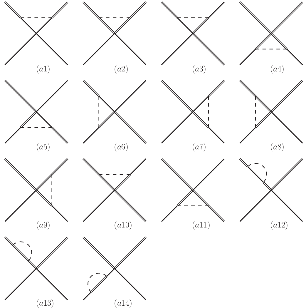


We now focus on the contact contributions first (Fig. 2). Involved vertexes are contact interaction (7), interaction (1) and interaction (5). Combined with defined flavor wave function (III), their isospin amplitudes can be written as
| (17) | ||||
| (18) | ||||
| (19) | ||||
| (20) | ||||
| (21) | ||||
| (22) | ||||
| (23) | ||||
| (24) | ||||
| (25) | ||||
| (26) | ||||
| (27) | ||||
| (28) | ||||
| (29) |
In the above, still takes for . is the space-time dimension coming from the dimensional regularization. and are constants depending on different diagrams and isospin , which are collected in Table I. Also, in these expressions and are the abbreviations of the polarization vectors and respectively. Each is a loop function defined in Refs. Liu:2012vd; Xu:2017tsr. For following OPE and TPE amplitudes these notations apply.
Notice that, one should further expand these amplitudes (17)-(29), later variables and (embed in the constants ) in them have to be replaced as the following:
| (30) |
Then we consider the OPE contributions showing in Fig. 3. To describe , , and vertexes, we utilize the chiral Lagrangians (1) and (5). According to the flavor wave function (III) the corresponding isospin amplitudes are
| (31) | ||||
| (32) | ||||
| (33) | ||||
| (34) | ||||
| (35) | ||||
| (36) | ||||
| (37) | ||||
| (38) | ||||
| (39) | ||||
| (40) | ||||
| (41) | ||||
| (42) |
where is a constant depending on each diagram and isospin , and we collect them in Table II. Note that in Eq. (42), stands for the tree-level OPE amplitude (Eq. (15) or Eq. (16)) where the pion decay constant has been replaced by correction .
Final pieces are the TPE contributions depicted in Fig.4. Here we need , , and vertexes. Using the chiral Lagrangians (1) and (5), the isospin amplitudes of TPE are written by
| (43) | ||||
| (44) | ||||
| (45) | ||||
| (46) | ||||
| (47) | ||||
| (48) | ||||
| (49) | ||||
| (50) | ||||
| (51) | ||||
| (52) |
where , , and are constants collected in Table III.
Notice that in above amplitudes (17)-(52), loop functions , , , and are abbreviated as , , , and , respectively. Respective constants and for different diagrams are listed in Tables I-III. These loop functions are calculated using dimensional regularization, with the modified minimal subtraction scheme.
Besides one loop diagrams in Figs. 2-4, at this order tree-level amplitudes also emerge. For example, there are contact contributions that come from contact Lagrangians (8)-(10). The LECs in Eqs. (8)-(10) actually consist of two parts: The finite parts that will intrduce large amounts of unknown parameters, and the divergent parts which are used to renormalize the 1-loop diagrams. In this work, the finite parts of the LECs in Eq. (8)-(10) are ignored due to the lack of fitting data available.
In our work, we consider -wave interactions, therefore we have following substitutions for the terms related to the polarization vectors:
| (53) | |||
| (54) |
After calculating the scattering amplitudes of systems in four different channels, the potentials in momentum space can be obtained via relation:
| (55) |
In this work, we aim to investigate weather the interactions are strong enough to form molecular states, therefore we are interested in potentials at coordinate space. With the help of Fourier transformation we can get potentials :
| (56) |
Because are polynomial in , the integral will be highly divergent with the increasing of the order. Here we renormalize the potential by introducing a Gaussian cutoff exp with as in Ref. Xu:2017tsr.
IV Numerical results and Discussions
In this section, we first discuss the parameters and the LECs appearing in our calculations. Then we substitute calculated potentials into the Schrödinger equation and explore weather the interactions are strong enough to form bound states. Later we discuss calculated potentials in detail.
In this work, we use the following parameters: GeV, - mass splitting GeV, the decay constant GeV, the renormalization scale and the bare coupling as in Ref. Xu:2017tsr. In our paper we ignore the isospin breaking in the isospin doublet .
For the LECs , , and in Eq. (7), we lack available data that can be fitted, so we use the resonance saturation to estimate the LECs. With the expressions in appendix A, we obtain: , , and .
IV.1 Bound state properties of
We first investigate weather interactions are strong enough to form bound states. the system has the quantum numbers and , i.e., there are four channels: , , and channels.
For the reliability of our investigation, we will leave the cutoff parameter undetermined. Generally, in nucleon-nucleon ChEFT, is adopted below meson mass Epelbaum:2014efa. Also, in our previous work, we used GeV Xu:2017tsr. In this paper, we will vary the cutoff at vicinity of GeV to search for the bound state solutions, where a relatively wide range will be adopted.
We solve the Schrödinger equations with the potentials (56). We present the dependences of calculated masses, the binding energies and the root-mean-square (RMS) radii in Table IV. In Table IV, with ranging from to GeV, we can see that there are various bound state solutions appearing in considered channels:
| GeV | ||||||||||||
|---|---|---|---|---|---|---|---|---|---|---|---|---|
For the channel, the bound state solution appears at GeV, and becomes deeper with increasing . But it then disappears at 1.0 GeV. The binding energy varies from MeV which is within one order of magnitude. As for the RMS radius, we can see that except large radius (9.0 fm) at GeV, the radius is basically around 2 fm. Therefore, it is interesting to see that, our obtained bound state solution in this channel is stable against the variation of .
In a word, in our HMChEFT calculations, the interaction in the channel is strong enough to form a bound state. In this channel we have a loosely bound state with the mass around 3872 MeV, the binding energy MeV and the RMS radius about fm. This solution just corresponds to , so our estimates indicate that indeed may be treated as a good candidate of molecular state. Or we can say interactions is strongly responsible for .
We now focus on the channel. In Table IV, there exists a shallow bound state solution within only a narrow range GeV. The binding energy is MeV which is quite small. Consequently, the solution has a large radius with around fm. Similarly, this solution is also stable against the variation of . So we conclude that in the channel, the binding between is relatively weaker comparing to the above, but their interaction is still strong enough to form a shallow bound state.
In this channel, there is no bound state solutions in the all range ( GeV). Combining with the bound state property in the channel discussed below, we conclude that the interaction in is weakest among all four channels.
For the channel, we can find a bound state solution beginning with a relatively large cutoff GeV. Different from the solutions in previous
channels, in this channel, the binding energy just becomes deeper and deeper with increasing . At GeV, we have the binding energy MeV with the RMS radius
fm. Because of the large cutoff needed to produce the bound state, we can say that the binding in the channel is weaker than that in the and
channels.
In general, we find that strongest binding of the system is in the channel, the next is in the channel, then in the channel, the final is
in the .
IV.2 The behaviors of the potentials
In previous subsections, we explore the bound state properties in the four channels. We find that with some reasonable cutoffs, there will emerge bound state solutions. Some of them are even stable against the variation of . In this section, to give a deep understandings of the bound state properties and the interactions, we further discuss the behaviors of the potentials .
Back to Table IV, we see around GeV the solution in the channel is close to most. For a more delicate investigation, here we set the cutoff to be GeV after fitting the mass of . With this cutoff we now present of all channels in Fig. 5.

For the channel, we see that the OPE and contact contributions are attractive, where the former is relatively weak. While the TPE contribution provides a strong repulsive force. Our numerical estimate reveals that with the increase of the cutoff , the attractive contributions as well as the repulsive TPE contribution all become stronger, however their cancellation just leads to a stable total potental . That is why calculated binding energy in Table IV is stable.
In the channel, the behaviors of the contact and TPE contributions do not differ from those in the channel above, whereas the OPE contribution changes to be repulsive. So, they lead to a weaker attraction comparing to the channel. That explains why the binding energy in this channel is always smaller than that in the channel (see the binding energies in Table IV).
For the channel, the OPE contribution is repulsive while the contact and TPE contributions are attractive. The cancellation between them makes the line shape of the total basically follows the line shape of the contact potential. Observing the amount of the total , we see that although attractive, it is not strong enough comparing to the amount in or channel.
At the channel in Fig. 5, all the contributions are attractive. However at the middle range GeV-1, the total is repulsive, which originates from the repulsion of the TPE. This causes the attraction of the channel to be weakened. Indeed, there is no bound state solution at . Also, from Table IV we see that a considerably high is needed to produce a bound state solution.
In general, through analyzing the potentials depicted in Fig. 5, we have understood the specific mechanism of the bound state formation in each channel. Depend on the distinct behaviors of the contact, OPE and TPE contributions in the four channels, the total s all present attractive line shapes but with different strengths. We find that most attractive potential is in the channel, then in the , then in the , the final is in the channel.
Combining with the discussions of the biding energies in Sec. IV.1, we conclude that there is a hierarchy of the strengths in the interactions:
| (57) |
where str. stands for the strength of the interaction. Note that despite discrepancies in details, this conclusion is consistent with the one-boson-exchange model calculations Liu:2008tn; Zhao:2014gqa; Wang:2021aql.
IV.3 and molecular states
In previous two sections, we point out the strength ordering in the interactions. But that does not means they can all produce bound states. From Table IV we already fond that only the , and channels have solutions. In this section we focus on the and channels which have no direct experimental indications.
As discussed in Sec. IV.1, the solution with mass around MeV in the channel just corresponds to . That means has a strong relation to the interaction, or, is a good candidate of the molecular state. In other two channels and , there also tends to form molecular states.
From Sec. IV.1, we have learned that in the channel, the shallow bound state solution has the binding energy MeV with GeV. Hence we plot the potential at GeV in Fig. 6. From Fig. 6, the OPE contribution is repulsive, therefore the binding of calculated molecular state is provided by the contact potential after the cancellation between the contact and TPE contributions. Also, we can see that the attraction is mainly provided in a range round GeV-1.

In other channel , we have a molecular state with considerable binding energy at GeV. Its potential is depicted in Fig. 7. All contributions are attractive, but the binding is mainly provided by the TPE contribution. Also, it is a basically short range attraction.

In general, the and molecular states have different binding mechanisms under the competitions of various contact, OPE and TPE contributions. As we know, experiment has not observe any possible structures that can fit into our predicted and molecular candidates yet, so we briefly discuss their discovery potentials.
We first focus on their decay patterns. The state has possible two body hidden charm decay channels and . It can also have three body strong decays such as and . In other possible channels such as , and , the signal can be overwhelmed by . It may also have baryonic decay channel , radiative decay channels , , and .
The state has possible two body hidden charm decay channels , , and , three body decay channels , , , , baryonic decay channel , and radiative decay channels , , and . It has more decay channels than the state, so its decay width may be larger.
These two possible molecular states can be produced in various production mechanisms. For example, they can be searched through subsequent decays in the collision at BESIII and BelleII experiments. It is also promising to collect them in decay processes such as .
In fact, some decay channels listed above have already been measured in experiment. For example, is the discovery channel of famous Ablikim:2013mio; Liu:2013dau; BESIII:2015cld; Abazov:2018cyu. It is possible that our state is the neutral component of isovector , although there exists discrepancy in mass. On the other hand, if the state is different from , there may exist more than one enhancements around GeV in the invariant mass spectrum. However because of the limited resolution in the invariant mass distributions of Refs. Ablikim:2013mio; Liu:2013dau; BESIII:2015cld; Abazov:2018cyu; Belle:2014nuw; LHCb:2019maw we can not pin down this issue now. We hope more sophisticated studies in future can clarify this problem. As for the and channel, no structures are found around GeV so far.
The , which the molecular state decays into, has also been studied in experiment. In 2004, measured the invariant mass spectrum of the in the process BaBar:2004iez. In the mass distribution of Fig. 8, we can see that there seems to have a peak around threshold. In the measurement of Ref. Belle:2013vio, a small enhancement also can be seen in their invariant mass spectrum. These enhancements may relate to our predicted molecular state. A weak sign appears in the invariant mass spectrum in Ref. Belle:2015yoa too. However, in these experiments the events around this region are limited, we hope experiments can pay more attention on these channels, especially the in the future.

In addition, measured kaon momentum spectrum in BaBar:2019hzd. signal is located around GeV. With more refined data in the future, we hope there will emerge fine structures if our predicted and states exist.
Other production mechanisms such as the low energy collision at ANDA are also promising. The and states can be produced through the or channel in the scattering.
V Summary
In our previous paper Xu:2017tsr, we studied the double charmed system in the framework of heavy meson chiral effective field theory (HMChEFT). We applied obtained chiral interactions to exotic state investigations. Predicted molecular state is consistent with the latest finding LHCb:2021vvq. In present work, we extend it to investigate the charmed-anticharmed system . As mentioned in Sec. I, various states were observed around open-charm thresholds, therefore the elaborate heavy-meson interactions studied here may help us to reveal the formations of these charmonium-like states.
The generalization of previous work is not straightforward. So we first construct interaction Lagrangians by properly considering charge conjugation properties of the fields in the heavy quark limit. We then calculate -wave potentials up to order at 1-loop level using weinberg’s scheme. The complete contact, one pion exchange (OPE) and two pion exchange (TPE) interactions are included. For a deeper understanding of the interactions, we further solve the Schrödinger equations using calculated potentials.
The behaviors of the potentials as well as bound state properties are analyzed in detail. In considered four channels i.e. , , and , there appears distinct behaviors depending on the competitions of the contact, OPE and TPE interactions. This leads to the specific mechanism of the bound state formation in each channel. For example, in the and channels, relatively large repulsions of the TPE contributions cause them to have weak bindings.
Combining the potential behaviors and the bound state properties, we conclude that there exists a strength ordering of the interactions in the four channels which would lead to different binding abilities:
| (58) |
where str. stands for the strength of the interaction.
Further, our investigation reveals that the interaction in the channel is strongly responsible for in experiment, in specific, can be a good candidate of the molecular state. In addition, there also tends to form molecular states in the and channels.
We examine the potential behaviors of the and molecular states in detail, point out their formation mechanisms. Their discovery potentials are also discussed. We hope future experiments such as BESIII, LHCb and BelleII can further study them in the productions and -decays, to search for the predicted multi-structures around the mass region. We also expect that they can be searched in future ANDA experiment.
Acknowledgments
We thank Fu-Lai Wang, Zhan-Wei Liu and Xiang Liu for helpful discussions. This work is supported by the National Natural Science Foundation of China (NSFC) under Grant No. 12005168.
Appendix A Determination of the unknown LECs
Assuming contact contributions from Eq. (7) are equivalent to , and exchanges, we will be able to extract , , and .
For , and exchanges, we need corresponding interacting Lagrangians for vertex:
| (59) | ||||
| (60) |
as well as their charge conjugations:
| (61) | ||||
| (62) |
where and
In above, and has been defined in Eq. (II) and (II), , and GeV-1 Li:2012ss, Bardeen:2003kt.
By matching the amplitudes in the two ways, we get
| (66) |
References
- (1) R. Aaij et al. (LHCb Collaboration), Observation of structure in the -pair mass spectrum, Sci. Bull. 65, 1983 (2020).
- (2) R. Aaij et al. (LHCb Collaboration), Amplitude analysis of the decay, Phys. Rev. D 102, 112003 (2020).
- (3) R. Aaij et al. (LHCb Collaboration), Observation of an exotic narrow doubly charmed tetraquark, arXiv:2109.01038 [hep-ex].
- (4) H. X. Chen, W. Chen, X. Liu and S. L. Zhu, The hidden-charm pentaquark and tetraquark states, Phys. Rept. 639, 1 (2016).
- (5) A. Esposito, A. Pilloni and A. D. Polosa, Multiquark Resonances, Phys. Rept. 668, 1 (2017).
- (6) R. F. Lebed, R. E. Mitchell and E. S. Swanson, Heavy-Quark QCD Exotica, Prog. Part. Nucl. Phys. 93, 143 (2017).
- (7) F. K. Guo, C. Hanhart, U. G. Meiner, Q. Wang, Q. Zhao and B. S. Zou, Hadronic molecules, Rev. Mod. Phys. 90, 015004 (2018).
- (8) Y. R. Liu, H. X. Chen, W. Chen, X. Liu and S. L. Zhu, Pentaquark and Tetraquark states, Prog. Part. Nucl. Phys. 107, 237 (2019).
- (9) N. Brambilla, S. Eidelman, C. Hanhart, A. Nefediev, C. P. Shen, C. E. Thomas, A. Vairo and C. Z. Yuan, The states: experimental and theoretical status and perspectives, Phys. Rept. 873, 1 (2020).
- (10) S. K. Choi et al. (Belle Collaboration), Observation of a narrow charmonium-like state in exclusive decays, Phys. Rev. Lett. 91, 262001 (2003).
- (11) S. Godfrey and N. Isgur, Mesons in a Relativized Quark Model with Chromodynamics, Phys. Rev. D 32, 189 (1985).
- (12) M. Ablikim et al. (BESIII Collaboration), Observation of a Charged Charmoniumlike Structure in at =4.26 GeV, Phys. Rev. Lett. 110, 252001 (2013).
- (13) Z. Q. Liu et al. (Belle Collaboration), Study of and Observation of a Charged Charmonium-like State at Belle, Phys. Rev. Lett. 110, 252002 (2013). Erratum: [Phys. Rev. Lett. 111, 019901 (2013)].
- (14) M. Ablikim et al. (BESIII Collaboration), Observation of a Charged Charmoniumlike Structure and Search for the in , Phys. Rev. Lett. 111, 242001 (2013).
- (15) K. Abe et al. (Belle Collaboration), Observation of a near-threshold omega mass enhancement in exclusive decays, Phys. Rev. Lett. 94, 182002 (2005).
- (16) T. Aaltonen et al. (CDF Collaboration), Evidence for a Narrow Near-Threshold Structure in the Mass Spectrum in Decays, Phys. Rev. Lett. 102, 242002 (2009).
- (17) S. K. Choi et al. (Belle Collaboration), Observation of a resonance-like structure in the mass distribution in exclusive decays, Phys. Rev. Lett. 100, 142001 (2008).
- (18) S. Jia et al. (Belle Collaboration), Observation of a vector charmoniumlike state in , Phys. Rev. D 100, 111103 (2019).
- (19) S. Jia et al. (Belle Collaboration), Evidence for a vector charmoniumlike state in , Phys. Rev. D 101, 091101 (2020).
- (20) F. L. Wang, X. D. Yang, R. Chen and X. Liu, Correlation of the hidden-charm molecular tetraquarks and the charmoniumlike structures existing in the process, Phys. Rev. D 104, 094010 (2021).
- (21) S. Weinberg, Nuclear forces from chiral Lagrangians, Phys. Lett. B 251, 288 (1990).
- (22) S. Weinberg, Effective chiral Lagrangians for nucleon - pion interactions and nuclear forces, Nucl. Phys. B 363, 3 (1991).
- (23) C. Ordonez and U. van Kolck, Chiral lagrangians and nuclear forces, Phys. Lett. B 291, 459 (1992).
- (24) C. Ordonez, L. Ray and U. van Kolck, The Two nucleon potential from chiral Lagrangians, Phys. Rev. C 53, 2086 (1996).
- (25) E. Epelbaum, W. Gloeckle and U. G. Meissner, Nuclear forces from chiral Lagrangians using the method of unitary transformation. 1. Formalism, Nucl. Phys. A 637, 107 (1998).
- (26) E. Epelbaum, W. Gloeckle and U. G. Meissner, Nuclear forces from chiral Lagrangians using the method of unitary transformation. 2. The two nucleon system, Nucl. Phys. A 671, 295 (2000).
- (27) M. P. Valderrama, Perturbative renormalizability of chiral two pion exchange in nucleon-nucleon scattering, Phys. Rev. C 83, 024003 (2011).
- (28) M. Pavon Valderrama, Perturbative Renormalizability of Chiral Two Pion Exchange in Nucleon-Nucleon Scattering: P- and D-waves, Phys. Rev. C 84, 064002 (2011).
- (29) B. Long and C. J. Yang, Renormalizing chiral nuclear forces: a case study of , Phys. Rev. C 84, 057001 (2011).
- (30) B. Long and C. J. Yang, Short-range nuclear forces in singlet channels, Phys. Rev. C 86, 024001 (2012).
- (31) X. W. Kang, J. Haidenbauer and U. G. Meissner, Antinucleon-nucleon interaction in chiral effective field theory, JHEP 1402, 113 (2014).
- (32) E. Epelbaum, H. Krebs and U. G. Meissner, Improved chiral nucleon-nucleon potential up to next-to-next-to-next-to-leading order, Eur. Phys. J. A 51, 53 (2015).
- (33) B. Long and Y. Mei, Cutoff regulators in chiral nuclear effective field theory, Phys. Rev. C 93, 044003 (2016).
- (34) L. Y. Dai, J. Haidenbauer and U. G. Meissner, Antinucleon-nucleon interaction at next-to-next-to-next-to-leading order in chiral effective field theory, JHEP 07, 078 (2017).
- (35) K. W. Li, T. Hyodo and L. S. Geng, Strangeness baryon-baryon interactions in relativistic chiral effective field theory, Phys. Rev. C 98, 065203 (2018).
- (36) X. L. Ren, K. W. Li, L. S. Geng, B. W. Long, P. Ring and J. Meng, Leading order relativistic chiral nucleon-nucleon interaction, Chin. Phys. C 42, 014103 (2018).
- (37) Y. Xiao, L. S. Geng and X. L. Ren, Covariant chiral nucleon-nucleon contact Lagrangian up to order , Phys. Rev. C 99, 024004 (2019).
- (38) S. Wu and B. Long, Perturbative scattering in chiral effective field theory, Phys. Rev. C 99, 024003 (2019).
- (39) V. Baru, E. Epelbaum, J. Gegelia and X. L. Ren, Towards baryon-baryon scattering in manifestly Lorentz-invariant formulation of SU(3) baryon chiral perturbation theory, Phys. Lett. B 798, 134987 (2019).
- (40) X. L. Ren, E. Epelbaum and J. Gegelia, -nucleon scattering in baryon chiral perturbation theory, Phys. Rev. C 101, 034001 (2020).
- (41) Z. Liu, L. H. Wen and J. F. Yang, Covariant propagator and chiral power counting, Nucl. Phys. B 963, 115288 (2021).
- (42) Q. Q. Bai, C. X. Wang, Y. Xiao and L. S. Geng, Pion-mass dependence of the nucleon-nucleon interaction, Phys. Lett. B, 135745 (2020).
- (43) Y. Xiao, C. X. Wang, J. X. Lu and L. S. Geng, Two-pion exchange contributions to the nucleon-nucleon interaction in covariant baryon chiral perturbation theory, Phys. Rev. C 102, 054001 (2020).
- (44) C. X. Wang, L. S. Geng and B. Long, Renormalizability of leading order covariant chiral nucleon-nucleon interaction, Chin. Phys. C 45, 054101 (2021).
- (45) E. Epelbaum, H. W. Hammer and U. G. Meissner, Modern Theory of Nuclear Forces, Rev. Mod. Phys. 81, 1773 (2009).
- (46) R. Machleidt and D. R. Entem, Chiral effective field theory and nuclear forces, Phys. Rept. 503, 1 (2011).
- (47) R. Machleidt and F. Sammarruca, Chiral EFT based nuclear forces: Achievements and challenges, Phys. Scripta 91, 083007 (2016).
- (48) U. G. Meissner, The long and winding road from chiral effective Lagrangians to nuclear structure, Phys. Scripta 91, 033005 (2016).
- (49) E. Epelbaum, H. Krebs and P. Reinert, High-precision nuclear forces from chiral EFT: State-of-the-art, challenges and outlook, Front. in Phys. 8, 98 (2020).
- (50) Z. W. Liu, N. Li and S. L. Zhu, Chiral perturbation theory and the strong interaction, Phys. Rev. D 89, 074015 (2014).
- (51) H. Xu, B. Wang, Z. W. Liu and X. Liu, potentials in chiral perturbation theory and possible molecular states, Phys. Rev. D 99, 014027 (2019).
- (52) B. Wang, Z. W. Liu and X. Liu, interactions in chiral effective field theory, Phys. Rev. D 99, 036007 (2019).
- (53) L. Meng, B. Wang, G. J. Wang and S. L. Zhu, The hidden charm pentaquark states and interaction in chiral perturbation theory, Phys. Rev. D 100, 014031 (2019).
- (54) B. Wang, L. Meng and S. L. Zhu, Spectrum of the strange hidden charm molecular pentaquarks in chiral effective field theory, Phys. Rev. D 101, 034018 (2020).
- (55) B. Wang, L. Meng and S. L. Zhu, Hidden-charm and hidden-bottom molecular pentaquarks in chiral effective field theory, JHEP 11, 108 (2019).
- (56) L. Meng, B. Wang and S. L. Zhu, interaction in chiral effective field theory, Phys. Rev. C 101, 064002 (2020).
- (57) B. Wang, L. Meng and S. L. Zhu, interaction and the structure of and in chiral effective field theory, Phys. Rev. D 101, 094035 (2020).
- (58) K. Chen, B. Wang and S. L. Zhu, Exploration of the doubly charmed molecular pentaquarks, Phys. Rev. D 103, 116017 (2021).
- (59) Y. R. Liu, X. Liu, W. Z. Deng and S. L. Zhu, Is Really a Molecular State?, Eur. Phys. J. C 56, 63-73 (2008).
- (60) X. Liu, Z. G. Luo, Y. R. Liu and S. L. Zhu, X(3872) and Other Possible Heavy Molecular States, Eur. Phys. J. C 61, 411-428 (2009).
- (61) N. Li and S. L. Zhu, Isospin breaking, Coupled-channel effects and Diagnosis of X(3872), Phys. Rev. D 86, 074022 (2012).
- (62) L. Zhao, L. Ma and S. L. Zhu, Spin-orbit force, recoil corrections, and possible and molecular states, Phys. Rev. D 89, 094026 (2014).
- (63) A. De Rujula, H. Georgi and S. L. Glashow, Molecular Charmonium: A New Spectroscopy?, Phys. Rev. Lett. 38, 317 (1977).
- (64) N. A. Tornqvist, From the deuteron to deusons, an analysis of deuteronlike meson-meson bound states, Z. Phys. C 61, 525 (1994).
- (65) C. Y. Wong, Molecular states of heavy quark mesons, Phys. Rev. C 69, 055202 (2004).
- (66) E. S. Swanson, Short range structure in the , Phys. Lett. B 588, 189 (2004).
- (67) M. B. Voloshin, Interference and binding effects in decays of possible molecular component of , Phys. Lett. B 579, 316 (2004).
- (68) F. E. Close and P. R. Page, The threshold resonance, Phys. Lett. B 578, 119 (2004).
- (69) N. A. Tornqvist, Isospin breaking of the narrow charmonium state of Belle at 3872 MeV as a deuson, Phys. Lett. B 590, 209 (2004).
- (70) M. Suzuki, The boson: Molecule or charmonium, Phys. Rev. D 72, 114013 (2005).
- (71) Y. J. Zhang, H. C. Chiang, P. N. Shen and B. S. Zou, Possible S-wave bound-states of two pseudoscalar mesons, Phys. Rev. D 74, 014013 (2006).
- (72) C. E. Thomas and F. E. Close, Is a molecule?, Phys. Rev. D 78, 034007 (2008).
- (73) I. W. Lee, A. Faessler, T. Gutsche, and V. E. Lyubovitskij, as a molecular state in a potential model, Phys. Rev. D 80, 094005 (2009).
- (74) G. J. Ding, J. F. Liu and M. L. Yan, Dynamics of Hadronic Molecule in One-Boson Exchange Approach and Possible Heavy Flavor Molecules, Phys. Rev. D 79, 054005 (2009).
- (75) Z. F. Sun, J. He, X. Liu, Z. G. Luo and S. L. Zhu, and as the and molecular states, Phys. Rev. D 84, 054002 (2011).
- (76) Z. F. Sun, Z. G. Luo, J. He, X. Liu and S. L. Zhu, A note on the , , , , molecular states, Chin. Phys. C 36, 194-204 (2012).
- (77) J. He, Study of the bound states in a Bethe-Salpeter approach, Phys. Rev. D 90, 076008 (2014).
- (78) Y. C. Yang, Z. Y. Tan, J. Ping and H. S. Zong, Possible and molecular states in the extended constituent quark models, Eur. Phys. J. C 77, 575 (2017).
- (79) Z. Y. Wang, J. J. Qi, X. H. Guo and C. Wang, as a molecular state in the Bethe-Salpeter equation approach, Phys. Rev. D 97, 016015 (2018).
- (80) B. X. Sun, D. M. Wan and S. Y. Zhao, The interaction with isospin zero in an extended hidden gauge symmetry approach, Chin. Phys. C 42, 053105 (2018).
- (81) Z. M. Ding, H. Y. Jiang and J. He, Molecular states from and interactions, Eur. Phys. J. C 80, 1179 (2020).
- (82) G. Burdman and J. F. Donoghue, Union of chiral and heavy quark symmetries, Phys. Lett. B 280, 287 (1992).
- (83) M. B. Wise, Chiral perturbation theory for hadrons containing a heavy quark, Phys. Rev. D 45, R2188 (1992).
- (84) T. M. Yan, H. Y. Cheng, C. Y. Cheung, G. L. Lin, Y. C. Lin and H. L. Yu, Heavy quark symmetry and chiral dynamics, Phys. Rev. D 46, 1148 (1992), Erratum: [Phys. Rev. D 55, 5851 (1997)].
- (85) M. Ablikim et al. (BESIII Collaboration), Observation of in , Phys. Rev. Lett. 115, 112003 (2015).
- (86) V. M. Abazov et al. (D0 Collaboration), Evidence for in semi-inclusive decays of -flavored hadrons, Phys. Rev. D 98, 052010 (2018).
- (87) K. Chilikin et al. (Belle Collaboration), Observation of a new charged charmoniumlike state in decays, Phys. Rev. D 90, 112009 (2014).
- (88) R. Aaij et al. (LHCb Collaboration), Model-Independent Observation of Exotic Contributions to Decays, Phys. Rev. Lett. 122, 152002 (2019).
- (89) B. Aubert et al. ( Collaboration), Observation of the decay and search for , Phys. Rev. Lett. 93, 041801 (2004).
- (90) T. Iwashita et al. (Belle Collaboration), Measurement of branching fractions for decays and search for a narrow resonance in the final state, PTEP 2014, 043C01 (2014).
- (91) A. Vinokurova et al. (Belle Collaboration), Search for B decays to final states with the meson, JHEP 06, 132 (2015), Erratum: [JHEP 02, 088 (2017)].
- (92) J. P. Lees et al. ( Collaboration), Measurements of the Absolute Branching Fractions of , Phys. Rev. Lett. 124, 152001 (2020).
- (93) N. Li, Z. F. Sun, X. Liu and S. L. Zhu, Coupled-channel analysis of the possible and molecular states, Phys. Rev. D 88, 114008 (2013).
- (94) W. A. Bardeen, E. J. Eichten and C. T. Hill, Chiral multiplets of heavy - light mesons, Phys. Rev. D 68, 054024 (2003).