Mitigation of Crosstalk Errors in Quantum Measurements

In this section, we collect notations and terminologies to be used throughout. In a noiseless scenario, a measurement on a single-qubit state is performed in the computational basis, in which measurement operators are given as

A general measurement that can describe noisy cases is denoted by a positive-operator-valued-measure (POVM). Let $\Pi_{0}$ and $\Pi_{1}$ denote POVM elements of a noisy measurement giving outcomes $0$ or $1$,

Note also that, throughout, a measurement is complete; hence, we only have outcomes $0$ or $1$. Then, a POVM element of a noiseless measurements on multiple qubits giving outcomes $\vec{a}=a_{1}a_{2}\cdots a_{n}$ where $a_{i}\{0,1\}$ for $i=1,\cdots,n$ is given by,

One can also rephrase a noiseless measurement as an estimation of $n$-qubit observables $Z_{1}\otimes Z_{2}\otimes\cdots\otimes Z_{n}$ where $Z_{j}=|0\rangle\langle 0|-|1\rangle\langle 1|$ for all $j=1,\cdots,n$.

In a realistic scenario, let $\Pi_{\vec{a}}$ denote a POVM giving outcomes $\vec{a}$. A measurement contains crosstalk noise if it cannot be decomposed into a product form, i.e.,

The right-hand-side above describes a noisy POVM element that does not contain crosstalk noise.

To quantify noisy POVM elements, it is generic to estimate their distinguishability with noiseless instances,

for a relevant distance measure such as $1$-norm. We here restrict the consideration to the chosen basis, see noiseless measurement in Eq. (1). The quantification of a noisy POVM element from its ideal realization is computed by the fidelity,

It is clear that if $\Pi_{\vec{a}}$ forms a noiseless measurement, we have $F(\Pi_{\vec{a}})=1$ for all $\vec{a}$. Otherwise, we have $F(\Pi_{\vec{a}})<1$.

Although the above quantification is commonly used to characterize error, the resulting estimate does not capture only single-measurement error but also crosstalk error. Measurement crosstalk noise can be identified when a POVM element of a joint measurement cannot be characterized by separated measurement devices.

For simplicity, let us consider measurements on two qubits denoted by $S_{1}$ and $S_{2}$. QDT is performed on a two-qubit joint measurement and verifies a POVM element, denoted by $\Pi_{a_{1}a_{2}}$. Let us also consider QDT performed on individual measurements with the corresponding POVM elements, denoted by $\Pi_{a_{1}}$ and $\Pi_{a_{2}}$. One can conclude that measurement crosstalk exists when a POVM element $\Pi_{a_{1}a_{2}}$ is not a product of them,

When crosstalk noise is present, measurement outcomes of individual qubits cannot be independent. We introduce the gap as follows,

and note that

Since measurement crosstalk noise concerns correlations between measurements of individual qubits, we introduce a measure for the crosstalk [13],

where the minimization runs over all POVM elements $M_{a_{1}}$ and $M_{a_{2}}$. We have used $\|X\|_{2}:=\sigma_{max}(X)$ where $\sigma_{max}(X)$ is the maximal singular value of $X$. Note that $\mathcal{C}(\Pi_{a_{1}a_{2}})=0$ if and only if a POVM element on two qubits can be factorized. When computing the crosstalk measure, one can exploit a Kraus operator parameterized as follows,

for the optimization of POVM elements $M_{i}=K^{\dagger}_{i}K_{i}$.

In Table I, the measure for measurement crosstalk noise is computed in the fake backend ‘FakeBrisbane’ that mimics real QPU ‘ibm_brisbane’, see Fig. 1. QDT is performed on multiple qubits, three pairs of qubits $(67,66)$, $(67,63)$, and $(67,60)$. A two-qubit state $|00\rangle$ is prepared, and the probability of having outcomes $00$ is collected. The probabilities are $0.890$, $0.895$, and $0.886$, respectively, for the three pairs. The crosstalk noise $C(\Pi_{00})$ is computed, which can also decrease by quantum preprocessing that applies a local unitary $U$, i.e., $\mathcal{C}(U^{\dagger}\Pi_{00}U)<\mathcal{C}(\Pi_{00})$, where an optimal local unitary can be constructed, see Subsection III-B.

As a prerequisite, let us suppose that QDT is performed on $n$-qubit measurements. A POVM element

is thus provided, from which we construct local unitaries for preprocessing and classical postprocessing. We refer to two decompositions of a POVM element, one we call preferred-basis decomposition (PBD), which is for Protocol 1, and the other eigendecomposition (ED) for Protocol 2.

The goal is clearly to approximate an outcome probability from noisy measurements into that of a noiseless one. A mitigation protocol, denoted by $\mathrm{MIT}$, signifies a method to minimize a distance in the following: for a $n$-qubit state $\rho$,

where $\mathrm{tr}[\rho|\vec{a}\rangle\!\langle\vec{a}|]$ denotes a probability of $\vec{a}$ that can be obtained by a noiseless measurement.

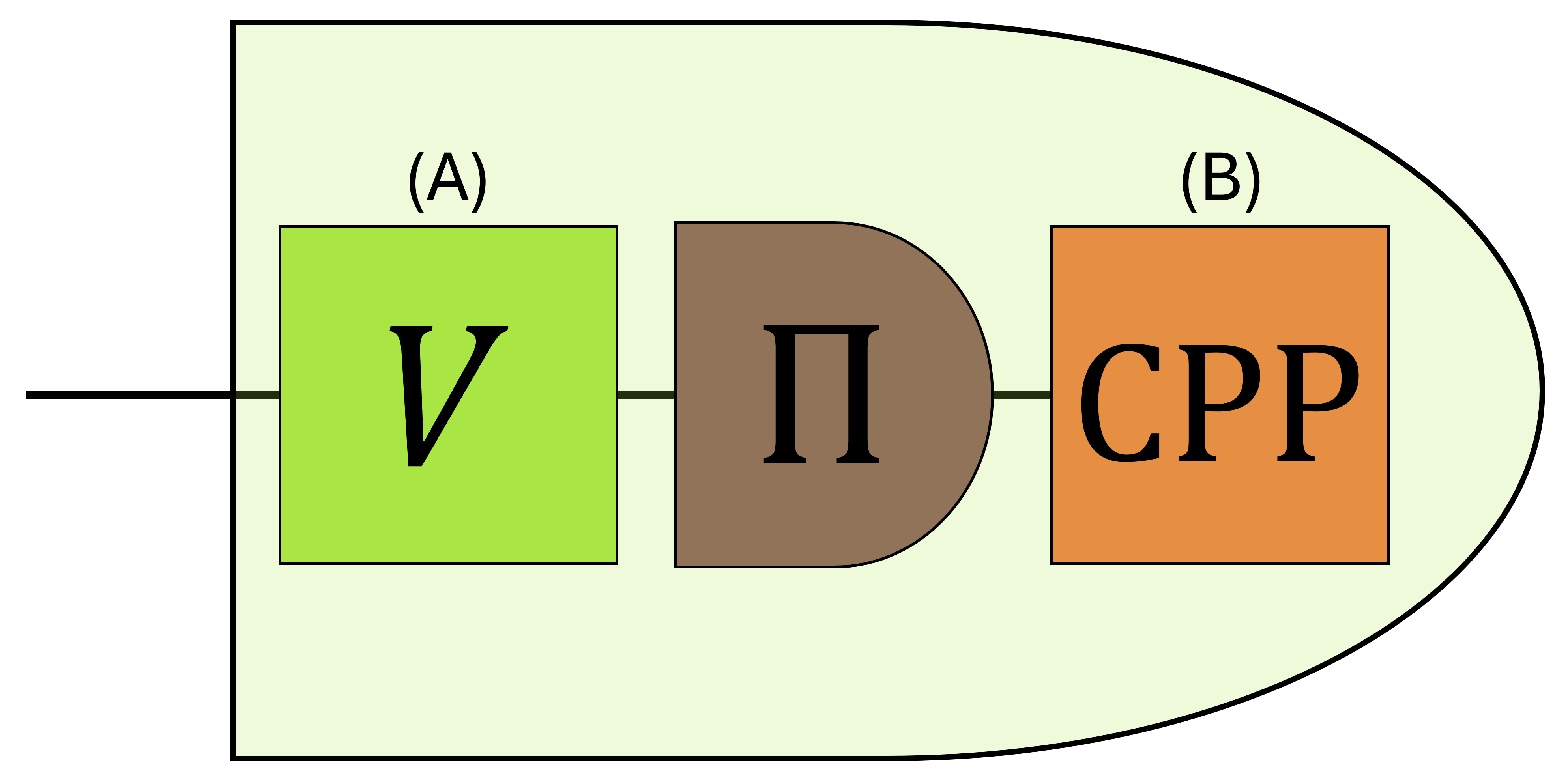
We devise a protocol $\mathrm{MIT}$ such that it contains local unitaries that have lower error rates than measurements. For instance, superconducting qubits show a measurement error rate ten times higher than a single-qubit gate. Thus, the motivation of the mitigation protocol is to consume single-qubit gates, with much fewer errors and more feasible with present-day quantum technologies, to suppress measurement errors. The flow of mitigation protocols we propose is summarized in Fig. 4.

We here exploit a PBD of a POVM element as follows,

where $|\vec{a}\rangle$ is a preferred basis and $P_{\vec{a}}$ is a Hermitian operator corresponding to the difference between noisy and noiseless POVM elements.

The quantum preprocessing (QPP) is to exploit a local unitary transform $V$ before a noisy measurement

where $v_{i}$ denotes a local unitary for the $i$-th qubit. An application of a unitary $V$ before a noisy measurement takes place, see Fig. 2, can be seen equivalently as a transformation of a POVM element as follows,

with the preferred basis $|\vec{a}\rangle$ and $Q_{\vec{a}}$ is a Hermitian operator corresponding to a difference between two operators $V^{\dagger}\Pi_{\vec{a}}V$ and $|\vec{a}\rangle\langle\vec{a}|$, see also Eq. (10).

The reason to exploit a local unitary $V$ is to increase the fidelity of a noisy POVM element as follows,

Then, a unitary transform $V$ that increases the fidelity is thought,

This also means that $\langle\vec{a}|Q_{\vec{a}}|\vec{a}\rangle\leq\langle\vec{a}|P_{\vec{a}}|\vec{a}\rangle$, see Fig. 3.

The classical postprocessing (CPP) can be devised once a measurement is performed with a POVM element in Eq. (12). Let us write by

and it holds that

from which a probability from a noiseless measurement is given by

Note that $\widetilde{q}(\vec{a})$ is given from measurements but $\mathrm{tr}[Q_{\vec{a}}\rho]$ is not known; while $Q_{\vec{a}}$ has been verified by QDT of a noisy measurement, $\mathrm{tr}[Q_{\vec{a}}\rho]$ cannot be computed immediately for an unknown state $\rho$. As it is bounded by $(Q_{\vec{a}})_{\min}$ and $(Q_{\vec{a}})_{\max}$, we make an approximation as its average:

Here, the maximum and minimum eigenvalues of $Q_{\vec{a}}$ are written by:

Finally, as $(Q_{\vec{a}})_{\min}$ and $(Q_{\vec{a}})_{\max}$ are closer, the resulting probability $p(\vec{a})$ makes a better approximation to a noiseless one $p_{0}(\vec{a})$. For this reason, we find a local unitary in QPP such that the difference is minimized,

where $Q_{\vec{a}}=V^{\dagger}\Pi_{\vec{a}}V-|\vec{a}\rangle\langle\vec{a}|$. Protocol 1 is summarized in $\mathrm{Algorithm}$ 1.

Let us now show that Protocol 1 derives a resulting probability distribution which is $\epsilon$-close to a noiseless probability, i.e., $\left|p(\vec{a})-p_{0}(\vec{a})\right|=O(10^{-2})$. First, we note that $|\bar{Q}_{\vec{a}}|=O(10^{-2})$ since it is a product of decimals

where $|\mathrm{tr}Q_{\vec{a}}|=|1-\mathrm{tr}\Pi_{\vec{a}}|<1$ from Eq. (12) and, clearly, $|{\bar{Q}_{\vec{a}}}/{\mathrm{tr}Q_{\vec{a}}}|<1$. The difference between a noiseless probability and a mitigated one can be found from Eqs. (16) and (17), and we compute,

The right-hand side can be rewritten as,

where $|\mathrm{tr}Q_{\vec{a}}|=|1-\mathrm{tr}\Pi_{\vec{a}}|<1$ from Eq. (12), and also clearly the next term is less than $1$. Hence, we have an estimate $\left|p(\vec{a})-p_{0}(\vec{a})\right|=O(10^{-2})$. We remark that the rate of suppression is independent of the number of qubits; hence, for any $n$-qubit measurement, Procotol 1 can suppress a measurement error rate up to a percentage level.

Protocol 2 exploits an eigendecomposition (ED) of a POVM element as follows,

where $\{\alpha_{i}^{[\vec{a}]}\}$ are eigenvalues which are sorted in descending order; $\alpha_{1}^{[\vec{a}]}\geq\alpha_{i}^{[\vec{a}]}\geq\cdots\geq\alpha_{d}^{[\vec{a}]}$ and thus $P_{\vec{a}}=\sum_{i=2}^{d}\alpha_{i}^{[\vec{a}]}|\alpha_{i}^{[\vec{a}]}\rangle\!\langle\alpha_{i}^{[\vec{a}]}|$. Protocol 2 also contains the QPP and the CPP, where the QPP finds a local unitary $V$ such that

Thus, a local unitary $V$ realizes a best approximation to a rotation of a basis $|\alpha_{1}^{[\vec{a}]}\rangle$ to a desired one $|a\rangle$.

Once an optimal local unitary $V$ is verified, the next steps of the QPP and the CPP are straightforward. The QPP applies a local unitary $V$ to realize a transformation of a POVM element,

Note that the eigenvalues of $P_{\vec{a}}$ remain the same under a local unitary $V$. A probability of measurement outcomes is bounded above and below as follows,

where we have written

It is straightforward to derive the upper bound from Eq. (23),

Protocol 2 is summarized in $\mathrm{Algorithm}$ 2. Following the lines in Eq. (20), we have $\Delta\bar{P}_{\vec{a}}=O(10^{-2})$ and thus the upper bound of the error, $\Delta\bar{P}_{\vec{a}}/\alpha_{1}^{[\vec{a}]}$, is also in the order of $10^{-2}$.

As a realistic scenario, the QPP and the CPP are implemented in the fake backend ‘FakeBrisbane’ that mimics the real QPU ‘ibm_brisbane’, see Fig. 1. In Table II, qubits labeled $66$ and $67$ are considered. From the results of QDT, the fidelities of POVM elements are obtained $F(\Pi_{0})$, which increase by a local unitary $U$. From decompositions in Eqs. (10) and (12), we also compute $\Delta\bar{P}_{0}=((P_{0})_{\max}-(P_{0})_{\min})/2$ and $\Delta\bar{Q}_{0}=((Q_{0})_{\max}-(Q_{0})_{\min})/2$.

Local unitaries on $n$ qubits are denoted by $V=\bigotimes_{i=1}^{n}v_{i}$ where $v_{i}$ for $i=1,\cdots,n$ is a single-qubit unitary. A single-qubit unitary can be parametrized by $(\theta,\phi,\lambda)$,

QDT is performed on single-, two-, and three-qubit measurements. For instance, POVM elements $\Pi_{0}$ of single-qubit measurements, giving outcome $0$, for qubits labeled $66$ and $67$ are obtained:

and

In Table II, their fidelities are listed as well as the improvement by local unitaries and properties of $P$ and $Q$ operators of Protocol 1.

QDT is also performed on two qubits labeled $67$ and $66$ and reconstructed a POVM element

from which we have the probability of having outcomes $00$ is $0.890$. We also compute the crosstalk measure in Eq. (8) and obtain $0.093$. Note that a noiseless POVM element is $\mathrm{diag}[1,0,0,0]$.

We here apply Protocols 1 and 2 to mitigate measurement errors on multiple qubits. We also consider two protocols in the following scenarios: (i) mitigation of noisy measurements for a specific outcome and (ii) mitigation of noisy measurements for all outcomes on average. Both scenarios have distinct applications in quantum information processing. For instance, protocols such as quantum entanglement distillation or static error purification [7] rely only on specific outcomes.

References

- [1] (2022) Noisy intermediate-scale quantum algorithms. Rev. Mod. Phys. 94, pp. 015004. External Links: Document Cited by: §I, §VI.
- [2] (2024) A review on quantum approximate optimization algorithm and its variants. Physics Reports 1068, pp. 1–66. External Links: Document Cited by: §I.
- [3] (2019) Detector tomography on ibm quantum computers and mitigation of an imperfect measurement. Phys. Rev. A 100, pp. 052315. External Links: Document Cited by: §I.
- [4] (2021) Conditionally rigorous mitigation of multiqubit measurement errors. Phys. Rev. Lett. 127, pp. 090502. External Links: Document Cited by: §I.
- [5] (2020) Rigorous measurement error correction. Quantum Sci. Technol. 5, pp. 03LT01. External Links: Document Cited by: §I.
- [6] (1997) Stabilizer codes and quantum error correction. arXiv:quant-ph/9705052. Cited by: §I.
- [7] (2025) Protocol for purifying noisy preparation and measurements of qubits. arXiv:2508.16136. Cited by: §V-B.
- [8] (2021) A hybrid quantum-classical approach to mitigating measurement errors in quantum algorithms. IEEE Trans. Comput. 70 (9), pp. 1401–1411. External Links: Document Cited by: §I, §VI.
- [9] (2022) Deep-neural-network discrimination of multiplexed superconducting-qubit states. Phys. Rev. Appl. 17, pp. 014024. External Links: Document Cited by: §I.
- [10] (2020) Mitigation of readout noise in near-term quantum devices by classical post-processing based on detector tomography. Quantum 4, pp. 257. Cited by: §I.
- [11] (2021) Experimental characterization of crosstalk errors with simultaneous gate set tomography. PRX Quantum 2, pp. 040338. External Links: Document Cited by: §I.
- [12] (2020) Detecting crosstalk errors in quantum information processors. Quantum 4, pp. 321. Cited by: §I.
- [13] (2022) Measurement crosstalk errors in cloud-based quantum computing. IEEE Internet Computing 26 (1), pp. 26–33. External Links: Document Cited by: §II-B.
- [14] (1995) Scheme for reducing decoherence in quantum computer memory. Phys. Rev. A 52, pp. R2493–R2496. External Links: Document Cited by: §I.
- [15] (2022) The variational quantum eigensolver: a review of methods and best practices. Physics Reports 986, pp. 1–128. External Links: Document Cited by: §I.
- [16] (2023) Mitigating quantum errors via truncated neumann series. Sci. China Inf. Sci. 66 (8), pp. 180508. External Links: Document Cited by: §I.
![[Uncaptioned image]](2112.10651v2/scseo.jpg) |
Seungchan Seo received the B.E. degree in 2020 from Hanyang University, Seoul, Republic of Korea, and the M.S. degree in 2022 from the Korea Advanced Institute of Science and Technology (KAIST), Daejeon, Republic of Korea, where he is currently pursuing the Ph.D. degree. His research interests include quantum computing, quantum tomography, quantum benchmarking, and verification of quantum devices. |
![[Uncaptioned image]](2112.10651v2/jhseong.jpg) |
Jiheon Seong received the B.E. degree in 2018 and the M.S. degree in 2020 from the Korea Advanced Institute of Science and Technology (KAIST), Daejeon, Republic of Korea, where he is currently pursuing the Ph.D. degree. His research interests include entanglement theory, entanglement measures, quantum resource theories, and the implementation and verification of entanglement on quantum hardware platforms. |
![[Uncaptioned image]](2112.10651v2/hyku.jpg) |
Huan-Yu Ku received the B.Sc., M.Sc. and Ph.D. degrees in physics from National Cheng-Kung University, Tainan, Taiwan, in 2013 ,2015, and 2019, respectively. From 2014 to 2015, he was a visiting student at Riken, Japan. He has been a Post-Doctoral Research Fellow from 2019 to 2022 at National Cheng-Kung University and from 2022 to 2023 at The Institute for Quantum Optics and Quantum Information (IQOQI), Vienna, Austria. He is currently an Assistant Professor of physics National Taiwan Normal University. His research interests include quantum information, quantum foundations, optimization problems, and quantum resource distillation. |
![[Uncaptioned image]](2112.10651v2/jwbae.jpg) |
Joonwoo Bae (Member, IEEE) obtained a Ph.D. in Theoretical Physics from Universitat de Barcelona & ICFO-Institute of Photonic Sciences, Barcelona in 2007. He has worked at the Korea Institute for Advanced Study (KIAS), Centre for Quantum Technologies (CQT) in Singapore, the ICFO, Freiburg Institute for Advanced Studies (FRIAS) as a Junior Fellow, and Hanyang University. He is currently with the School of Electrical Engineering, Korea Advanced Institute of Science and Technology (KAIST). His research interests include secure quantum communication, entanglement applications, open quantum systems, quantum foundations, and their practical applications. |