DOI HERE \vol00 \accessAdvance Access Publication Date: Day Month Year \appnotesPaper \copyrightstatementPublished by Oxford University Press on behalf of the Institute of Mathematics and its Applications. All rights reserved.
P. Csomós, B. Farkas, and B. Kovács
[*]Corresponding author: balazs.kovacs@mathematik.uni-regensburg.de
042022 0Year 0Year
Error estimates for a splitting integrator for abstract semilinear boundary coupled systems
Abstract
We derive a numerical method, based on operator splitting, to abstract parabolic semilinear boundary coupled systems. The method decouples the linear components which describe the coupling and the dynamics in the abstract bulk- and surface-spaces, and treats the nonlinear terms similarly to an exponential integrator. The convergence proof is based on estimates for a recursive formulation of the error, using the parabolic smoothing property of analytic semigroups and a careful comparison of the exact and approximate flows. This analysis also requires a deep understanding of the effects of the Dirichlet operator (the abstract version of the harmonic extension operator) which is essential for the stable coupling in our method. Numerical experiments, including problems with dynamic boundary conditions, reporting on convergence rates are presented.
keywords
Lie splitting, error estimates, boundary coupling, semilinear problems.1 Introduction
In this paper we derive a Lie-type splitting integrator for abstract semilinear boundary coupled systems, and prove first order error estimates for the time integrator by extending the results of [11] from the linear case. The main idea of our algorithm is to decouple the two nonlinear problems appearing in the original coupled system, while maintaining stability of the boundary coupling with the help of the abstract Dirichlet operator. We use techniques from operator semigroup theory to prove the first-order convergence in the following abstract setting.
We consider the abstract semilinear boundary coupled systems of the form:
| (1.1) |
where , are linear operators on the Banach spaces and , respectively, , are suitable functions, and the two unknown functions and are related via the linear coupling operator acting between (subspaces of) and . The subscript in refers to the fact that this operator is maximal in a certain sense, this and the bulk–surface terminology is further explained in Example 1. A typical setting would be that is a trace-type operator between the space (for the bulk dynamics) and the boundary space (for the surface dynamics). The precise setting and assumptions for (1.1) will be described below.
This abstract framework simultaneously includes problems which have been analysed on their own as well. For instance, abstract boundary feedback systems, see [12], [13], [9] and the references therein, fit into the above abstract framework where the equations in and representing the bulk and boundary equations. Such examples arise, for instance, for the boundary control of partial differential equation systems, see [34, 35], and [33], [20, Section 3], and [1, Section 3]. These problems usually involve a bounded feedback operator acting on , which can be easily incorporated into the nonlinear term above. For regularity results we refer to these works. We further note, that semilinear parabolic equations with dynamic boundary conditions, see [53, 18, 23, 10, 51, 36, 46, 22, 32], etc., and diffusion processes on networks with boundary conditions satisfying ordinary differential equations in the vertices, see [40, 41, 47, 43, 42], etc., both formally fit into this setting. In both cases, however, the feedback operator is unbounded.
In this paper we propose, as a first step into this direction, a Lie splitting scheme for abstract semilinear boundary coupled systems, where the semilinear term is locally Lipschitz (and might include feedback). An important feature of our splitting method is that it separates the flows on and , i.e. separates the bulk and surface dynamics. This could prove to be a considerable computational advantage if the bulk and surface dynamics are fundamentally different (e.g. fast and slow reactions, linear–nonlinear coupling, etc.). In general, splitting methods simplify (or even make possible) the numerical treatment of complex systems. If the operator on the right-hand side of the initial value problem can be written as a sum of at least two suboperators, the numerical solution is obtained from a sequence of simpler subproblems corresponding to the suboperators. We will use the Lie splitting, introduced in [7], which, from the functional analytic viewpoint, corresponds to the Lie–Trotter product formula, see [50], [19, Corollary III.5.8]. Splitting methods have been widely used in practice and analysed in the literature, see for instance the survey article [38], and see also, e.g., [48, 31, 49, 29] and [21, 14, 15, 16, 3, 4, 5], etc. The latter group lists references which overcome order reduction of splitting schemes occurring for problems different form the boundary coupled system (1.1).
In particular, for semilinear partial differential equations (PDEs) with dynamic boundary conditions, two bulk–surface splitting methods were proposed in [32]. The numerical experiments of Section 6.3 therein illustrate that both of the proposed splitting schemes suffer from order reduction.
Recently, in [6], a first-order convergent bulk–surface Lie splitting scheme was proposed and analysed. In [6] parabolic PDEs with dynamic boundary conditions were considered, proving that the splitting based fully discrete method converges to the spatially semi-discrete finite element solution. For results on semilinear problems in particular see [6, Appendix A]. The following aspects separate the two approaches: Even though both methods are suitable for semilinear problems, here we consider abstract boundary coupled parabolic problems in a general operator theoretic setting, see (1.1) and Section 2, while [6] considers a particular family of PDEs on Lipschitz domains, see [6, Section 2]. The two Lie splittings are derived via substantially different theoretical approaches: The one herein is derived using semigroup theory and exponential integrators in Banach spaces, see Section 2, in contrast the method in [6] is derived based on the differential algebraic structure of the bulk–surface finite element semi-discretisation of a PDE (the resulting sub-flows are discretised using the implicit Euler method), see [6, Section 4]. Here, we assume local Lipschitz continuity of the nonlinearities, in [6, Theorem A.1] global Lipschitz continuity and a mild CFL condition were assumed. Regularity requirements are comparable, for more details see Remark 2. We note that both methods differ from the two splitting schemes proposed in [32]. We are not aware of any other splitting-type numerical approaches separating the “bulk” and “boundary” dynamics.
In the present work we start by the variation of constants formula and apply the Lie splitting to approximate the appearing linear operator semigroups. More precisely, we will identify three linear suboperators: two describing the dynamics in the bulk and on the surface, respectively, and one corresponding to the coupling. Then, either the solutions to the linear subproblems are known explicitly, or can be efficiently obtained numerically. We will show that the proposed method is first-order convergent for boundary coupled semilinear problems, it does not suffer from order reduction, and is therefore promising for PDEs with dynamic boundary conditions, cf. [32], see the experiment in Section 5.2. Due to the unbounded boundary feedback operator, our present analysis does not apply to this situation, however, our numerical experiments show first order convergence. We strongly believe that the developed techniques presented in this work provide further insight into the behaviour of operator splitting schemes of such problems. This is strengthened by our numerical experiments.
The convergence result is based on studying stability and consistency, using the procedure called Lady Windermere’s fan from [28, Section II.3], however, these two issues cannot be separated as in most convergence proofs, since this would lead to sub-optimal error estimates. Instead, the error is rewritten using recursion formula which, using the parabolic smoothing property (see, e.g., [19, Theorem II.4.6 (c)]), leads to an induction process to ensure that the numerical solution stays within a strip around the exact solution. A particular difficulty lies in the fact that the numerical method for the linear subproblems needs to approximate a convolution term in the exact flow [11], therefore the stability of these approximations cannot be merely established based on semigroup properties. Estimates from [11] together with new technical results yield an abstract first-order error estimate for semilinear problems (with a logarithmic factor in the time step), under suitable (local Lipschitz-type) conditions on the nonlinearities. By this analysis within the abstract setting we gain a deep operator theoretical understanding of these methods, which are applicable for all specific models (e.g. mentioned above) fitting into the framework of (1.1). Numerical experiments illustrate the proved error estimates, and an experiment for dynamic boundary conditions complement our theoretical results.
The paper is organised as follows. In Section 2 we introduce the used functional analytic framework, and derive the proposed numerical method. We also state our main result, namely, the first-order convergence, the proof of which along with error estimates takes up Sections 3 and 4. Finally, Section 5 presents numerical experiments illustrating and complementing our theoretical results.
2 Setting and the numerical method
We consider two Banach spaces and , sometimes referred to as the bulk and boundary space, respectively, over the complex field . The product space is endowed with the sum norm, or any other equivalent norm, rendering it a Banach space and the coordinate projections bounded. Elements in the product space will be denoted by boldface letters, e.g. for and . The norm on is simply denoted by , on the other hand, for brevity, we will drop the subscript from the and norms, as it will be always clear from the context which norm is meant. We employ the usual convention for the operator norm as well. Then we treat the nonlinearities, derive the numerical method, and present the main result of the paper.
General framework
We will now define the abstract setting for linear boundary coupled systems, established in [9], i.e. for (1.1) with and . We will also list all our assumptions on the linear operators in (1.1).
The following general conditions—collected using Roman numerals—will be assumed throughout the paper:
-
[9999]
- (i)
The (so-called maximal) operator is linear.
- (ii)
The linear operator is surjective and bounded with respect to the graph norm of on .
- (iii)
The restriction of to generates a strongly continuous semigroup on . The (linear) operator is invertible, i.e., the resolvent set of , (cf. [9, Lemma 2.2]).
- (iv)
The (linear) operator generates a strongly continuous semigroup on .
- (v)
The operator matrix is closed.
We recall from [9, Lemma 2.2] that is invertible, and its inverse, often called the Dirichlet operator, given by
| (2.1) |
is bounded, and (via ) that
Note that the range of the Dirichlet operator is almost disjoint from the domain of (they intersect in ). Therefore no matter how regular the initial conditions are, the action of serves as a barrier, and will result in the logarithmic loss in the error estimate for exact solutions of arbitrary smoothness.
Let us briefly recall the following example from [11] (see Examples 2.7 and 2.8 therein), which is also one of the main motivating examples of [9]; we refer also to [25, 24, 8] for facts concerning Lipschitz domains.
Example 1 (Bounded Lipschitz domains).
Let be a bounded domain with Lipschitz boundary , and .
-
[9]
- (a)
Consider the following operators: with domain (being the maximal, distributional Laplacian without boundary conditions), and the Dirichlet trace of on (see, e.g., [39, pp. 89–106]). Then is surjective and actually has a bounded right-inverse , which is the harmonic extension operator, i.e. for any the function solves (uniquely) the Poisson problem with inhomogeneous Dirichlet boundary condition . The operator is strictly negative, self-adjoint and generates the Dirichlet-heat semigroup on .
- (b)
In summary, we see that the abstract framework of [9], hence of this paper, covers interesting cases of boundary coupled problems on bounded Lipschitz domains.
We now turn our attention towards the semigroup, and its generator, corresponding to the linear problem. Consider the linear operator
| (2.2) |
For and define the convolution
| (2.3) |
For all we also define , and using integration by parts, see [9], we immediately write
| (2.4) |
We see that and are both linear operators on (and we note that they are bounded when is endowed with the graph norm ).
The next result, recalled from [9], characterizes the generator property of , which in turn is in relation with the well-posedness of (1.1), see Section 1.1 in [41].
Theorem 1 ([9, Theorem 2.7]).
Within this setting, let the operators , be as defined in (2.2) and (2.1), and suppose that is invertible. The operator is the generator of a -semigroup if and only if for each the operator extends to a bounded linear operator with its operator norm satisfying
| (2.5) |
The semigroup generated by is then given as
| (2.6) |
In other words, if the conclusion of Theorem 1 holds, then the linear problem is well-posed and the solution with initial value is given by the semigroup as .
We augment the list of general conditions (i)–(v) by further assuming:
-
[9999]
- (vi)
Additionally to also operator is invertible.
- (vii)
The operators and generate bounded analytic semigroups.
The operators appearing in Example 1 satisfy all of these conditions.
Remark 1.
-
[9]
- (a)
By Corollary 2.8 in [9] the assumption in (vii) implies that is the generator of an analytic -semigroup on .
- (b)
The invertibility of or is merely a technical assumption which slightly simplifies the proofs and assumptions, avoiding a shifting argument.
- (c)
In principle, one can drop the assumption of being the generator of an analytic semigroup. In this case minor additional assumptions on the nonlinearity are needed, and the error bound for the numerical method will look slightly differently. We will comment on this in Remark 2 below, after the proof of the main theorem.
- (d)
The fact that generates a bounded analytic semigroup implies the bound , see, e.g., [19, Theorem II.4.6 (c)].
The abstract semilinear problem
We now turn our attention to semilinear boundary coupled problems (1.1). In particular we will give our precise assumptions related to the solutions of the semilinear problem, and to the nonlinearity .
Assumptions 1.
The function , , is a mild solution of the problem (1.1), written on as
| (2.7) |
i.e. it satisfies the variation of constant formula:
| (2.8) |
We further assume that the exact solution has the following properties:
-
[99]
- (A1)
The function is Lipschitz continuous on the strip, for an ,
around the exact solution with constant .
- (A2)
The second component is Lipschitz continuous on , with constant .
- (A3)
For each , and (here denotes the projection onto the second component).
- (A4)
The second component along the solution satisfies for each , and
- (A5)
Furthermore, is differentiable and .
The local Lipschitz continuity in strip is ensured if is assumed to be locally Lipschitz continuous on bounded sets, see, e.g., [30] and [32]. Later in the convergence analysis we will show that the numerical solution stays sufficiently close to the exact solution. We further comment on these assumptions, and their relation to those in [6], after the proof in Remark 2. Later on in the convergence proof, we will directly reference these properties by their number ().
The numerical method
We are now in the position to derive the numerical method. For a time step , for all , we define the numerical approximation to via the following steps.
-
[Step 1.]
- 1.
We approximate the integral in (2.8) by an appropriate quadrature rule.
- 2.
In what follows we describe the numerical method by using first-order approximations in Steps 1–2, and show its first-order convergence. We note here that the application of a correctly chosen exponential integrator could be inserted as a preliminary step, see [30]. Since it eliminates the integral’s dependence on , the quadrature rule simplifies in Step 1. This approach, however, leads to the same numerical method as Steps 1–2.
Before proceeding as proposed, for all , we rewrite formula (2.8) at as
| (2.9) |
Now, according to Step 1, we approximate the integral by the left rectangle rule leading to
for any .
In Step 2, we apply the Lie splitting, which, according to [11], results in the approximation of the convolution operator by an appropriate (to be specified later). Altogether, we approximate the semigroup operators by
| (2.10) |
We remark that holds with the notations introduced in [11]:
This leads to the numerical method approximating at time :
| (2.11) |
with .
The actual form of operator depends on the underlying splitting method. Here, we will use the Lie splitting of the operator , proposed in [11, Section 3]. Notice that
i.e., the similarity transformation , diagonalizes the domain of the formally diagonal operator with non-diagonal domain by decoupling the two components, cf. (2.2). Indeed, if and only if , i.e., if , and . These hold if and only if (since ), (since ) and ; this proves that has diagonal domain, and also the above form of follows at once, since for one has . Now the prize to be paid for this diagonalization of the domain is the new unbounded term making upper triangular. Notice also that the decoupling via the similarity transformation changes the diagonal term into . This technique is an abstract operator theoretic version of homogenizing boundary conditions. Now, the splitting is given by with
and , , . It was shown in [11, Prop. 3.2.] that the operator parts, see [19, Section II.2.3], , and generate the strongly continuous semigroups11 1 Note that the domain of definition of the part is , and that, in fact, .
respectively, on . Then the application of the Lie splitting as leads to the formula (2.10) with
| (2.12) |
Thus, the Lie splitting transfers the coupled linear problem into the sequence of simpler ones. First we solve the equation on by using the original initial condition , then we propagate the solution by , which serves as an initial condition to the homogeneous problem on . To get an approximation at , the semilinear expressions and the terms coming from the “diagonalisation” should be treated. Then the whole process needs to be cyclically performed times.
We note that the approximation can also be obtained by using an appropriate convolution quadrature, i.e. by approximating from the left (at ) and from the right (at ).
Upon plugging in the splitting approximation (2.12) into the convolution , and by introducing the intermediate values
| (2.13a) | ||||
| the method (2.11) reads componentwise as | ||||
| (2.13b) | ||||
This formulation only requires two applications of the Dirichlet operator per time step. We point out that the two terms with the Dirichlet operator can be viewed as correction terms which correct the boundary values of the bulk-subflow along the splitting method.
The main result
We are now in the position to state the main result of this paper, which asserts first order (up to a logarithmic factor) error estimates for the approximations obtained by the splitting integrator (2.11) (with (2.12)), i.e. (2.13), separating the bulk and surface dynamics in and .
Theorem 2.
In the above setting, let be the solution of (1.1) subject to the conditions in Assumptions 1 and consider the approximations at time determined by the splitting method (2.11) (with (2.12)), or written in componentwise form (2.13). Then there exists a and such that for any time step we have at time the error estimate
| (2.14) |
The constant is independent of and , but depends on , on constants related to the semigroups and , as well as on the exact solution .
The proof of this result will be given in Section 4 below. In the next section we state and prove some preparatory and technical results needed for the error estimates.
Recall that the splitting method (2.11), written componentwise (2.13), decouples the bulk and surface flows, which can be extremely advantageous if the two subsystems behave in a substantially different manner. We remind that, when applied to PDEs with dynamic boundary conditions, naive splitting schemes suffer from order reduction, see [32, Section 6], and a correction in [6].
We make the following remark about the logarithmic factor in the above error estimate. Inequality (2.14) implies that for any we have with another constant . This amounts to saying that the proposed method has convergence order arbitrarily close to , and in fact this is also what the numerical experiments show. Indeed, numerical experiments in Section 5 illustrate and complement the first-order error estimates of Theorem 2, including an example with dynamic boundary conditions, without any order reductions.
3 Preparatory results
In this section we collect some general technical results which will be used later on in the convergence proof. After a short calculation, or by using the results in Section 3 of [11], we obtain
| (3.1) | ||||
see [11, equation (3.9)]. Now we are in the position to prove exponential bounds for the powers of .
Lemma 1.
Proof.
For the sum norm on the product space , we have
The exponential boundedness of the semigroups and , and the boundedness of directly yield
It remains to bound the term . We obtain
which completes the proof of the first statement.
If is a bounded analytic semigroup, then we improve the last estimate to
By putting the estimates together, the assertions follows. ∎
We recall the following lemma from [11].
Lemma 2 ([11, Lemma 4.4]).
There is a such that for every , for any , and for every we have
Using the above quadrature estimate we prove the following approximation lemma.
Lemma 3.
For and we have
Proof.
Lemma 4.
For we have
Proof.
Resorting to the Taylor expansion we have for that
which readily implies , and hence the assertion. ∎
Lemma 5.
Let be Lipschitz continuous and consider
Then for all we have
Here, by we denote the norm , where is the best Lipschitz constant of .
Proof.
For , we have
∎
Let and denote the projection onto the first and second coordinate in .
Lemma 6.
For there is a such that for every , we have
Proof.
We have
and the second asserted inequality follows at once.
On the other hand, for the first component
and we obtain
and the first inequality is also proved. ∎
Lemma 7.
For there is a such that for every , , , we have
Proof.
From (3.1) we obtain
where denote the four terms in the order of appearance. By Lemma 4
so we need to estimate . Since has the appropriate convolution form, Lemma 5 implies
Altogether we obtain
For and we have
To estimate we recall from the proof of Lemma 1 that (for ), so
Finally, the estimates for together yield the assertion. ∎
4 Proof of Theorem 2
The proof of our main result is based on a recursive expression for the global error, which involves the local error and some nonlinear error terms. The recursive formula is obtained using a procedure which is sometimes called Lady Windermere’s fan [28, Section II.3]; our approach is inspired by [44], [52, Chapter 3]. The local errors are weighted by , therefore a careful accumulation estimate—heavily relying on the parabolic smoothing property—is required. In order to estimate the locally Lipschitz nonlinear terms we have to ensure that the numerical solution remains in the strip (see Assumptions 1). This will be shown using an induction process, which is outlined as follows:
- •
We shall find and a constant such that for any if belong to the strip and , then
- •
Since is a constant independent of and , we can take sufficiently small such that for each we have , the width of the strip , therefore by the previous step we have .
- •
Since belongs to the strip and since and are independent of , the proof can be concluded by induction.
Within the proof we will use the following conventions: The positive constant comes from bounds for any of the analytic semigroups , , or : For each
| (4.1) |
Here the last estimate is usually referred to as the parabolic smoothing property of analytic semigroups, cf. Remark 1 (c). By we will denote a constant that is independent of the time step, but may depend on other constants (e.g. parameters of the problem) and on the exact solution (hence on the initial condition). Within a proof we shall indicate a possible increment of such appearing constants by a subscript: , etc.
Proof of Theorem 2.
For the local Lipschitz continuity of the nonlinearity , we will prove that the numerical solution remains in the strip around the exact solution using an induction argument.
We estimate the global error , at time , by expressing it using the local error as follows:
with the nonlinear difference term . By resolving the recursion we obtain
| (4.2) | ||||
Since we have , the last term vanishes.
We now start the induction process. Let us assume that the error estimate (2.14) holds for all with , i.e., for a independent of and , we have
| (4.3) |
Below, we will show that the same error estimate also holds for as well. We note that, via , the assumed error estimate trivially holds for .
We will now estimate the remaining terms of (4.2) in parts (i)–(iii), respectively. The estimates (4.3) for the past values for only appear in part (iii).
(i) We rewrite the local error by using the forms (2.9) and (2.11) of the exact and approximate solutions, respectively, and by Taylor’s formula and (A5) as
| (4.4) |
In what follows we will estimate the three terms separately.
We will bound the first term by using the boundedness of the semigroups and . Denote and write
Whence we conclude
The second term in (4.4) can be estimated by Lemma 6, and using (A4), as
While, using the exponential boundedness of and (A5), the third term in (4.4) is directly bounded by
Therefore, we finally obtain for the local error that
| (4.5) |
(ii) Since in each time step the local error is and we have time steps, a more careful analysis is needed for the the second term in (4.2). We first rewrite this term by the variation of constants formula (2.9) and the numerical method in the form (2.11):
| (4.6) | ||||
We rewrite the second term on the right-hand side of (4.6) using Taylor’s formula:
Combining the two identities above, for (4.6) we obtain:
| (4.7) | ||||
Finally, we combine the bounds (4.8), (4.9), (4.10), respectively, for , , then collecting the terms we obtain
| (4.11) | ||||
where we have used the parabolic smoothing property (4.1) of the analytic semigroup to estimate the factor by .
(iii) The errors in the nonlinear terms are estimated by using Lemma 1 and the local Lipschitz continuity of in the appropriate spaces (see (A1) and (A2)), in combination with the bounds (4.3) for the past, as
| (4.12) | ||||
recalling that and are the Lipschitz constants on , see Assumptions 1 (A1) and (A2). For the last inequality, we used here that belongs to the strip so that the Lipschitz continuity of can be used, see (A1) and (A2).
The global error (4.2) is bounded by the combination of the estimates (4.5), (4.11), and (4.12) from (i)–(iii), which altogether yield
| (4.13) | ||||
A discrete Gronwall inequality then implies
| (4.14) |
for , with the constant . Then for a sufficiently small such that for each we have , then and the error estimate (2.14) is satisfied for as well. Hence (4.3) holds even up to instead of . Therefore, by induction, the proof of the theorem is complete. ∎
Remark 2.
-
[9]
- (a)
Theorem 2 remains true, with an almost verbatim proof as above, if is merely assumed to be the generator of a -semigroup. This requires the following additional condition:
-
[99]
- (A5′)
The function is differentiable and .
-
- (b)
Time-dependent nonlinearities can also be allowed and the same error bound holds without essential modification of the previous proof. Of course, the conditions (A1), (A2), (A4), and (A5) in Assumption 1, involving and need to be suitably modified. For example the functions need to be uniformly Lipschitz for (and even this can be relaxed a little), and the function defined by needs to be differentiable, etc.
- (c)
The assumptions (A3) and (A4) involving the domain may seem a little restrictive. However, in some applications these conditions are naturally satisfied: For example if is finite dimensional (such is the case for finite networks, see [43] or [47]). At the same time, these conditions seem to be optimal in this generality, and play a role only in the local error estimate of the Lie splitting, i.e., in Lemma 2 and its applications. Indeed, at other places the conditions involving are not needed.
- (d)
5 Numerical experiments
To illustrate and complement the error estimates of Theorem 2, we have performed numerical experiments for Example 1. In order to allow for a direct comparison with other works from the literature, we performed the same numerical experiments which were performed in [32] and [6].
Let be the unit disk with boundary , with denoting the trace operator, and n denoting the outward unit normal field. Let us consider the boundary coupled semilinear parabolic partial differential equation (PDE) system and satisfying
| (5.1) |
where the two nonlinearities are specified later, and where the two inhomogeneities and are chosen such that the exact solutions are known to be and (which naturally satisfy ). The boundary coupled PDE system (5.1) fits into the abstract framework (1.1) in the sense of Example 1. We note that Theorem 2 still holds for (5.1) with the time-dependent inhomogeneities, see Remark 2 (b).
We performed numerical experiments using the splitting method (2.11), written componentwise (2.13), which is applied to the bulk–surface finite element semi-discretisation, see [17, 32], of the weak form of (5.1). The bulk–surface finite element semi-discretisation is based on a quasi-uniform triangulation of the continuous domain , such that the discrete boundary is also a sufficient good approximation of . By this construction the traces of the finite element basis functions in naturally form a basis on the boundary , i.e. forms a boundary element basis on . Since , the numerical and exact solutions are compared using the lift ℓ, given by , where is a suitable image of , see [17, Section 4.1.1]. For more details we refer to [17, Section 4 and 5], or [32, Section 3]. Altogether this yields the matrix–vector formulation of the semi-discrete problem, for the nodal vectors and ,
| (5.2) |
where and are the mass-lumped mass matrix and stiffness matrix for , and similarly and for the discrete boundary , while the nonlinearities and the inhomogeneities are defined accordingly. The discrete trace operator extracts the nodal values at the boundary nodes. For all these quantities we have used quadratures of sufficiently high order such that the quadrature errors are negligible compared to all other spatial errors. For mass lumping in this context, and for its spatial approximation properties, we refer to [32, Section 3.6].
The two semigroups in (2.13) are known, and are computed using the expmv Matlab package of Al-Mohy and Higham [2], in the above matrix–vector formulation (5.2) the (diagonal) mass matrices are transformed to the identity, i.e. , and similarly for , and all other terms. The numerical experiments were performed for this transformed system. In this setting the operator in (2.1) corresponds to the harmonic extension operator, which we compute here by solving a Poisson problem with inhomogeneous Dirichlet boundary conditions.
5.1 Convergence experiments
We present two convergence experiments for the above boundary coupled PDE system, with nonlinearities:
| (5.3a) | ||||||
| (5.3b) | ||||||
i.e. with an Allen–Cahn-type nonlinearity, and a mixing nonlinearity.
This first nonlinearity was chosen since both [32] and [6] have reported on numerical experiments for the same Allen–Cahn example and , hence the numerical experiments here are directly comparable to those referenced above. The second nonlinearity was chosen since it introduces some mixing between the bulk and boundary variables and . We note here that the our experiments only serve as an illustration to Theorem 2—and as comparison to the literature—since the nonlinearities in (5.3) do not satisfy (A1)–(A5).
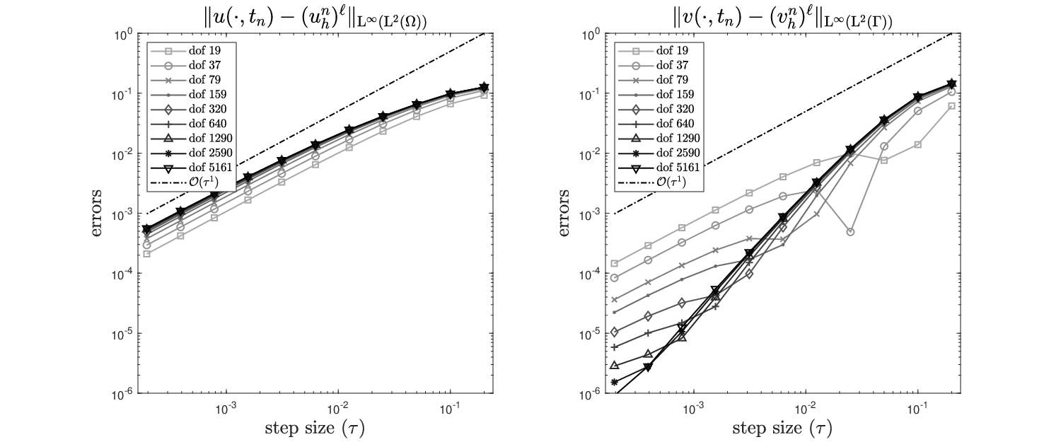
Using the splitting integrator (2.11), in the form (2.13), we have solved the transformed system (5.2) for a sequence of time steps (with ) and a sequence of meshes with mesh width .
In Figure 1 and 2 we report on the and errors of the two components for the two nonlinearities in (5.3), comparing the (nodal interpolation of the) exact solutions and the numerical solutions. Here, analogously to the norm on , for a sequence we set .) In the log-log plots we can observe that the temporal convergence order matches the predicted convergence rate of Theorem 2, note the dashed reference line (the factor is naturally not observable). In the figures each line (with different marker and colour) corresponds to a fixed mesh width , while each marker on the lines corresponds to a time step size . The precise time steps and degrees of freedom values are reported in Figure 1 and 2.
We are reporting on the fully discrete errors of the numerical solution on multiple spatial grids, to be able to observe clearly that the convergence order is not reduced in contrast to [32], cf. [32, Figure 2] where the error curves are sliding upward with each spatial refinement. Evidently, this is not the case here.
5.2 Convergence experiments with dynamic boundary conditions
We performed the same convergence experiment for a partial differential equation with dynamic boundary conditions, cf. [32, 6], let solve the problem
| (5.4) |
using the same domain, exact solution, nonlinearities, etc. as above.
Problem (5.4) is equivalently rewritten as a boundary coupled PDE system (5.1), where the two nonlinearities are given by
That is, the the nonlinear term incorporates the coupling through the Neumann trace . The numerical method (2.11), written componentwise (2.13), is applied to this formulation with the nonlinearity containing the Neumann trace operator.
We again report on convergence test with the nonlinearities (5.3) in the roles of and .
In Figure 3 and 4 we report on the and error of the bulk and surface errors for the two nonlinearities in (5.3), comparing the (nodal interpolation of the) exact solutions and the numerical solutions. (Figure 3 is obtained exactly as it was described for Figure 1, the precise time steps and degrees of freedom values can be read off from the figure.) Although in this case, due to the unboundedness of the Neumann trace operator in , the conditions of Theorem 2 are not satisfied, in Figure 3 we still observe a convergence rate (note the reference lines). Qualitatively we obtain the same plots for and norms.
Note that our splitting method does not suffer from any type of order reduction, in contrast to the splitting schemes proposed in [32], see Figure 1 and 2 therein. In [6] the same order reduction issue was overcome by a different approach, using a correction term.
Acknowledgments
The estimates within this paper were finalised during a Research in Pairs programme of all three authors at the Mathematisches Forschungsinstitut Oberwolfach (MFO). We are grateful for the Institute’s support—and for its unparalleled inspiring atmosphere.
Funding
Petra Csomós acknowledges the Bolyai János Research Scholarship of the Hungarian Academy of Sciences.
The work of Balázs Kovács is funded by the Heisenberg Programme of the Deutsche Forschungsgemeinschaft (DFG, German Research Foundation) – Project-ID 446431602, and by the DFG Graduiertenkolleg 2339 IntComSin – Project-ID 321821685.
The research was partially supported by the bilateral German-Hungarian Project CSITI – Coupled Systems and Innovative Time Integrators financed by DAAD and Tempus Public Foundation. This article is based upon work from COST Action CA18232 MAT-DYN-NET, supported by COST (European Cooperation in Science and Technology).
References
- Adler et al. [2017] M. Adler, M. Bombieri, and K.-J. Engel. Perturbation of analytic semigroups and applications to partial differential equations. J. Evol. Equ., 17(4):1183–1208, 2017. ISSN 1424-3199.
- Al-Mohy and Higham [2011] A. H. Al-Mohy and N. J. Higham. Computing the action of the matrix exponential, with an application to exponential integrators. SIAM J. Sci. Comput., 33(2):488–511, 2011. ISSN 1064-8275.
- Alonso-Mallo et al. [2018] I. Alonso-Mallo, B. Cano, and N. Reguera. Avoiding order reduction when integrating linear initial boundary value problems with exponential splitting methods. IMA J. Numer. Anal., 38:1294–1323, 2018.
- Alonso-Mallo et al. [2019] I. Alonso-Mallo, B. Cano, and N. Reguera. Avoiding order reduction when integrating reaction-diffusion boundary value problems with exponential splitting methods. J. Comput. Appl. Math., 357:228–250, 2019.
- Alonso-Mallo et al. [2021] I. Alonso-Mallo, B. Cano, and N. Reguera. Comparison of efficiency among different techniques to avoid order reduction with Strang splitting. Numer. Methods Partial Differential Equations, 37(1):854–873, 2021. ISSN 0749-159X. 10.1002/num.22556. URL https://doi.org/10.1002/num.22556.
- Altmann et al. [2022] R. Altmann, B. Kovács, and C. Zimmer. Bulk–surface Lie splitting for parabolic problems with dynamic boundary conditions. IMA Journal of Numerical Analysis, 2022. doi:10.1093/imanum/drac002.
- Bagrinovskii and Godunov [1957] K. A. Bagrinovskii and S. K. Godunov. Difference schemes for multidimensional problems. Dokl. Akad. Nauk. USSR, 115:431–433, 1957.
- Behrndt et al. [2020] J. Behrndt, F. Gesztesy, and M. Mitrea. Sharp boundary trace theory and Schrödinger operators on bounded Lipschitz domains. page 143 pages, 2020. preprint.
- Casarino et al. [2003] V. Casarino, K.-J. Engel, R. Nagel, and G. Nickel. A semigroup approach to boundary feedback systems. Int. Eq. Op. Th., 47(3):289–306, 2003.
- Colli and Fukao [2015] P. Colli and T. Fukao. The Allen–Cahn equation with dynamic boundary conditions and mass constraints. Math. Methods Appl. Sci. 0, 38(17):3950–3967, 2015.
- Csomós et al. [2021] P. Csomós, M. Ehrhardt, and B. Farkas. Operator splitting for abstract cauchy problems with dynamical boundary condition. Operators and Matrices, 15(3):903–935, 2021.
- Desch et al. [1985] W. Desch, I. Lasiecka, and W. Schappacher. Feedback boundary control problems for linear semigroups. Israel J. Math., 51(3):177–207, 1985.
- Desch et al. [2001] W. Desch, J. Milota, and W. Schappacher. Least square control problems in nonreflexive spaces. Semigroup Forum, 62(3):337–357, 2001.
- Einkemmer and Ostermann [2015] L. Einkemmer and A. Ostermann. Overcoming order reduction in diffusion-reaction splitting. Part 1: Dirichlet boundary conditions. SIAM J. Sci. Comput., 37(3):A1577–A1592, 2015. ISSN 1064-8275. 10.1137/140994204. URL https://doi.org/10.1137/140994204.
- Einkemmer and Ostermann [2016] L. Einkemmer and A. Ostermann. Overcoming order reduction in diffusion-reaction splitting. Part 2: Oblique boundary conditions. SIAM J. Sci. Comput., 38(6):A3741–A3757, 2016. ISSN 1064-8275. 10.1137/16M1056250. URL https://doi.org/10.1137/16M1056250.
- Einkemmer and Ostermann [2018] L. Einkemmer and A. Ostermann. A comparison of boundary correction methods for Strang splitting. Discrete Contin. Dyn. Syst. Ser. B, 23(7):2641–2660, 2018. ISSN 1531-3492. 10.3934/dcdsb.2018081. URL https://doi.org/10.3934/dcdsb.2018081.
- Elliott and Ranner [2013] C. M. Elliott and T. Ranner. Finite element analysis for a coupled bulk–surface partial differential equation. IMA J. Numer. Anal., 33(2):377–402, 2013.
- Engel and Fragnelli [2005] K.-J. Engel and G. Fragnelli. Analyticity of semigroups generated by operators with generalized Wentzell boundary conditions. Adv. Differential Equations, 10(11):1301–1320, 2005.
- Engel and Nagel [2000] K.-J. Engel and R. Nagel. One-parameter semigroups for linear evolution equations, volume 194 of Graduate Texts in Mathematics. Springer-Verlag, New York, 2000.
- Engel et al. [2010] K.-J. Engel, M. Kramar Fijavž, B. Klöss, R. Nagel, and E. Sikolya. Maximal controllability for boundary control problems. Appl. Math. Optim., 62(2):205–227, 2010. ISSN 0095-4616.
- Faou et al. [2015] E. Faou, A. Ostermann, and K. Schratz. Analysis of exponential splitting methods for inhomogenous parabolic equations. IMA J. Numer. Anal., 35:161–178, 2015.
- Gal [2007] C. G. Gal. Global well-posedness for the non-isothermal Cahn-Hilliard equation with dynamic boundary conditions. Adv. Differ. Equ., 12(11):1241–1274, 2007. ISSN 1079-9389.
- Gal and Grasselli [2008] C. G. Gal and M. Grasselli. The non-isothermal Allen-Cahn equation with dynamic boundary conditions. Discrete Cont. Dyn. Syst. Ser. A, 22:1009–1040, 2008. ISSN 1078-0947.
- Gesztesy and Mitrea [2008] F. Gesztesy and M. Mitrea. Generalized Robin boundary conditions, Robin-to-Dirichlet maps, and Krein-type resolvent formulas for Schrödinger operators on bounded Lipschitz domains. In Perspectives in partial differential equations, harmonic analysis and applications, volume 79 of Proc. Sympos. Pure Math., pages 105–173. Amer. Math. Soc., Providence, RI, 2008. URL https://doi.org/10.1090/pspum/079/2500491.
- Gesztesy and Mitrea [2011] F. Gesztesy and M. Mitrea. A description of all self-adjoint extensions of the Laplacian and Kreĭn-type resolvent formulas on non-smooth domains. J. Anal. Math., 113:53–172, 2011. ISSN 0021-7670. URL https://doi.org/10.1007/s11854-011-0002-2.
- Gesztesy et al. [2011] F. Gesztesy, I. Mitrea, D. Mitrea, and M. Mitrea. On the nature of the Laplace-Beltrami operator on Lipschitz manifolds. volume 172, pages 279–346. 2011. URL https://doi.org/10.1007/s10958-010-0199-0. Problems in mathematical analysis. No. 52.
- Haase [2006] M. Haase. The functional calculus for sectorial operators, volume 169 of Operator Theory: Advances and Applications. Birkhäuser Verlag, Basel, 2006.
- Hairer et al. [1993] E. Hairer, S. P. Nørsett, and G. Wanner. Solving ordinary differential equations. I, volume 8 of Springer Series in Computational Mathematics. Springer-Verlag, Berlin, 2nd edition, 1993.
- Hansen and Ostermann [2009] E. Hansen and A. Ostermann. Exponential splitting for unbounded operators. Math. Comp., 78(267):1485–1496, 2009.
- Hochbruck and Ostermann [2010] M. Hochbruck and A. Ostermann. Exponential integrators. Acta Numer., 19:209–286, 2010.
- Jahnke and Lubich [2000] T. Jahnke and C. Lubich. Error bounds for exponential operator splittings. BIT, 40(4):735–744, 2000.
- Kovács and Lubich [2017] B. Kovács and C. Lubich. Numerical analysis of parabolic problems with dynamic boundary conditions. IMA J. Numer. Anal., 37(1):1–39, 2017.
- Kumpf and Nickel [2004] M. Kumpf and G. Nickel. Dynamic boundary conditions and boundary control for the one-dimensional heat equation. J. Dynam. Control Systems, 10(2):213–225, 2004. ISSN 1079-2724.
- Lasiecka and Triggiani [2000a] I. Lasiecka and R. Triggiani. Control theory for partial differential equations: continuous and approximation theories. I, volume 74 of Encyclopedia of Mathematics and its Applications. Cambridge University Press, Cambridge, 2000a.
- Lasiecka and Triggiani [2000b] I. Lasiecka and R. Triggiani. Control theory for partial differential equations: continuous and approximation theories. II, volume 75 of Encyclopedia of Mathematics and its Applications. Cambridge University Press, Cambridge, 2000b.
- Liero [2013] M. Liero. Passing from bulk to bulk-surface evolution in the Allen–Cahn equation. Nonl. Diff. Eqns. Appl. (NoDEA), 20(3):919–942, 2013. ISSN 1420-9004.
- Lunardi [1995] A. Lunardi. Analytic semigroups and optimal regularity in parabolic problems. Modern Birkhäuser Classics. Birkhäuser/Springer Basel AG, Basel, 1995.
- McLachlan and Quispel [2002] R. I. McLachlan and G. R. W. Quispel. Splitting methods. Acta Numer., 11:341–434, 2002.
- McLean [2000] W. McLean. Strongly elliptic systems and boundary integral equations. Cambridge University Press, Cambridge, 2000. ISBN 0-521-66332-6; 0-521-66375-X.
- Mugnolo [2001] D. Mugnolo. A note on abstract initial boundary value problems. Tübinger Berichte zur Funktionalanalysis, 10:158–162, 2001.
- Mugnolo [2004] D. Mugnolo. Second order abstract initial-boundary value problems. PhD thesis, University of Tübingen, Tübingen, Germany, 2004.
- Mugnolo [2014] D. Mugnolo. Semigroup methods for evolution equations on networks. Understanding Complex Systems. Springer, Cham, 2014.
- Mugnolo and Romanelli [2007] D. Mugnolo and S. Romanelli. Dynamic and generalized Wentzell node conditions for network equations. Math. Methods Appl. Sci., 30(6):681–706, 2007.
- Ostermann et al. [2019] A. Ostermann, C. Piazzola, and H. Walach. Convergence of a low-rank Lie-Trotter splitting for stiff matrix differential equations. SIAM J. Numer. Anal., 57(4):1947–1966, 2019.
- Pazy [1983] A. Pazy. Semigroups of linear operators and applications to partial differential equations, volume 44 of Applied Mathematical Sciences. Springer-Verlag, New York, 1983.
- Racke and Zheng [2003] R. Racke and S. Zheng. The Cahn–Hilliard equation with dynamic boundary conditions. Adv. Differ. Equ., 8(1):83–110, 2003.
- Sikolya [2005] E. Sikolya. Flows in networks with dynamic ramification nodes. J. Evol. Equ., 5(3):441–463, 2005.
- Strang [1968] G. Strang. On the construction and comparison of difference schemes. SIAM J. Numer. Anal., 5(3):506–517, 1968.
- Thalhammer [2008] M. Thalhammer. High-order exponential operator splitting methods for time-dependent Schrödinger equations. SIAM J. Numer. Anal., 46(4):2022–2038, 2008.
- Trotter [1959] H. F. Trotter. On the product of semi-groups of operators. Proc. Amer. Math. Soc., 10:545–551, 1959.
- Vázquez and Vitillaro [2011] J. L. Vázquez and E. Vitillaro. Heat equation with dynamical boundary conditions of reactive–diffusive type. J. Differential Equations, 250(4):2143–2161, 2011.
- Walach [2019] H. Walach. Time integration for the dynamical low-rank approximation of matrices and tensors. PhD thesis, University of Tübingen, Tübingen, Germany, 2019.
- Wentzell [1959] A. D. Wentzell. On boundary conditions for multidimensional diffusion processes. Theor. Probab. Appl., 4(2):164–177, 1959.