A singular Riemannian geometry approach to Deep Neural Networks II. Reconstruction of 1-D equivalence classes.
Abstract
We proposed in a previous work a geometric framework to study a deep neural network, seen as sequence of maps between manifolds, employing singular Riemannian geometry. In this paper, we present an application of this framework, proposing a way to build the class of equivalence of an input point: such class is defined as the set of the points on the input manifold mapped to the same output by the neural network. In other words, we build the preimage of a point in the output manifold in the input space. In particular. we focus for simplicity on the case of neural networks maps from –dimensional real spaces to ()–dimensional real spaces, we propose an algorithm allowing to build the set of points lying on the same class of equivalence. This approach leads to two main applications: the generation of new synthetic data and it may provides some insights on how a classifier can be confused by small perturbation on the input data (e.g. a penguin image classified as an image containing a chihuahua). In addition, for neural networks from 2D to 1D real spaces, we also discuss how to find the preimages of closed intervals of the real line. We also present some numerical experiments with several neural networks trained to perform non-linear regression tasks, including the case of a binary classifier.
Keywords:
Deep Learning , Neural Network , Classification problem , Riemannian Geometry1 Introduction
Neural Networks (NN) have been acknowledged to be a very powerful tool in machine learning tasks: A not fully comprehensive list of such tasks includes as speech–to–text transcription [1, 2], image segmentation [3, 4], image classification [5], match new items and/or products with user’s interests [6], image morphing [7], imitation learning [8], solution to nonlinear PDEs [9, 10], image generation [11, 12]. The beginning of the new millennium has seen a growing interest in this automatic learning approach, due to the rising computational power (more performant GPUs) and the huge amount of data (the so-called Big Data Revolution). There exists several kind of neural networks, each one tailored for solving a particular problem: Some examples include Generative Adversarial Networks (GAN) [13] for the generation of new images, U–Net for image segmentation [14], Siamese Networks [15] for image matching. The majority of the previous techniques handles data and NN’s structures in an Euclidean framework: in this work we pursue our analysis by adopting a differential geometry approach. The idea that a neural network can be studied using differential geometry, working with non Euclidean data, is not new in literature [16, 17, 18, 19, 20, 21]. In particular in [20] and [18] it is shown that a fully connected neural network can be studied as a sequence of maps between manifolds, the latter focusing on the case of Riemannian manifolds. In [18] a notion of non-Euclidean distance between input points is proposed using a Riemannian metric tensor over the input manifold obtained employing the pullback of the Riemannian metric over the output manifold through the neural network map. However, the analysis carried out in [18] focus on the case of a sequence of manifolds of the same dimension, since they assume that the pullback of the Riemannian metric through the neural network is still a Riemannian metric – which is true only if the function realizing the neural network is a diffeomorphism: In general the resulting metric could be degenerate. To overcome this issue, we can assume to work in the setting of singular Riemannian geometry, in which the non-degeneracy of the metric is not assumed a priori. Starting from the ideas introduced in [18], in [22] we introduced a geometric framework to study fully connected neural networks with singular Riemannian geometry and we proved several results about neural networks seen as a finite sequence of maps between manifolds of the form
| (1) |
with the maps realizing the layers of the network (see definition 10) and being the input data manifold and the output manifold respectively. In the following we shall call the map the neural network map. In this paper, for a matter of simplicity, we work with a particular class of manifolds, that is nonetheless sufficient for applications, assuming that every manifold of the sequence (1) is either or a subset of . Note that this assumption is tantamount to require that every manifold admits a global coordinate system covering the whole set. Moreover, we consider a manifold only as an affine space and not as a vector space. As an affine space, differences between two point - or displacement vectors - are well defined and correspond to tangent vectors over . In particular, we can identify with for every [23].
Using this framework, we propose a way to build the class of equivalence of an input point, defined as the set of the points on the input manifold mapped to the same result by the neural network or, in other words, we build the preimage in of for a given point . Focusing, for simplicity, on the case of neural networks from subsets of to subsets of , we propose an algorithm which allows to build a curve of points lying on the same class of equivalence and we present some numerical experiments in the case of a neural network trained to perform non-linear regression. The study of these equivalence classes may provide useful insights on the misbehaviour of some neural classifier: indeed, a small noise perturbation on the input data may lead the NN to completely misclassify even a simple image. For example, in [24, Figure 1] a king penguin image is perturbed by a small amount of noise: such perturbation leads the classifier to label such noisy image as a chihuahua image. A further possible application is the generation of new synthetic data: indeed, the equivalence class constructed by the proposed procedure contains all the points classified with a particular label. Exploring this equivalence class may lead to find reliable and realistic new samples of the considered class.
In addition we also implement – in the case of a final manifold which is a subset of the real line – an algorithm allowing to explore the input manifold changing equivalence class at each step, which in turn allow us to find the preimage for a given closed interval .
The structure of the paper is the following. In Section 2 we recall some notions of differential and singular Riemannian geometry, mainly to fix the notation we employ in this work. Then, following [22] we introduce a geometric framework to analyse neural networks. In particular we consider a neural network as a finite sequence of maps between Riemannian manifolds satisfying certain properties stated in Section 3 and we discuss the link between classes of equivalence of a neural networks and singular Riemannian geometry, using the results of [22]. Then in Section 4 we introduce the one dimensional Singular Metric Equivalence Class algorithm (SiMEC) to build the class of equivalence of an input element. We introduce then the one dimensional Singular Metric Exploring algorithm (SiMExp) and we discuss how to employ both SiMEC and SiMExp to build the subset such that , , or in other words, to find the preimage of , a feature which is useful to study classifiers, since we can find all the points which are classified in the same way. Section 5 is devoted to present some numerical experiments: the first set of experiments regard the SiMEC algorithm, where we apply our framework to a fully connected neural network trained to perform a nonlinear regression, learning some functions from to , or equivalently learning some surfaces in from a cloud of points. In the second part of this section we extend the previous tests to the SiMExp algorithm, including an application to binary classification, in which we build an approximate separating surface. The code employed to run these numerical experiments can be found at http://github.com/alessiomarta/simec-1d-test-code.
Notations
The set of positive real numbers is denoted with , while denotes the set of non-negative real numbers. is the tangent space of the smooth manifold over the point and is the tangent bundle of the smooth manifold . The space of the bilinear forms over the vector space valued in is . stands for the length of a curve , while is the pseudolenght of a curve . Analogously, is distance between the points and and is pseudodistance between the points and . denotes the dimension of a manifold (or vector space) . is the kernel of the matrix (or metric) , while is the set of all finite linear combinations of elements if . Given a function , is its Jacobian matrix. denotes the pullback of the smooth map .
2 Geometric preliminaries
2.1 Basic notions in differential geometry
In this section we briefly recall some basic notions in differential geometry we employ in the rest of the paper. The details can be found in any standard textbook about differential geometry, e.g. [23] [25]. See also [22] for a more complete review of the background material. We begin reviewing the notion of smooth manifold, a generalization of the concept of surface in . We remember that a topological space is Hausdorff (or ) if for any two points , then there are two sets and such that ; A topological space is called second countable if it admits a countable basis.
Definition 1.
A smooth d-dimensional manifold is a second countable and Hausdorff topological space such that every point has a neighbourhood that is homeomorphic to through a map , with the additional requirement that if , then is a smooth diffeomorphism.
The pair is called a local chart and the collection of all the possible local charts at all points is an atlas. If we can cover the whole manifold with a chart, it will be called a global chart. The definition given above is not the most general one, but it is sufficient for our purposes. Indeed, in the following we are interested in smooth manifolds of the form , . Any subset of the Euclidean space with this form is diffeomorphic to and admits a global chart inherited from , for example the Cartesian coordinates restricted to . Given a function between two smooth manifold and , we say that is smooth if for any choice of local charts of and respectively, the function is smooth in the usual sense. In the case is a function between two subsets of two Euclidean spaces and , , this definition is tantamount to require that the components of the map are smooth. A notable example of function over manifolds is a curve over a manifold , namely a smooth function , .
In practice, describing a manifold giving an atlas or (when possible) a global chart is not always simple. A common (and simpler) way to build a manifold is to embed it in a higher dimensional space. For example we can realize the unit sphere – a 2-dimensional manifold – as the subset of – a 3-dimensional manifold with the usual Cartesian coordinates – such that and we say that we embedded in . If we describe a manifold as a subset of the Euclidean space , we say that is embedded in , whose in turn is called embedding space. The map realizing as a subspace of is called embedding. In general the definition of embedding from a manifold to a manifold is the following.
Definition 2.
Let be a smooth map between manifolds. is an embedding if its differential is everywhere injective and if it is an homeomorphism with its image. In other words, is a diffeomorphism with its image.
The next notion we need to recall is that of tangent space, a generalization of the tangent plane to a two-dimensional surface. For our purposes, it is convenient to define this geometric object using tangent vectors to curves over . Let and consider a chart containing . Consider two smooth curves such that . We say that is equivalent to at if (see [22, Figure 1]).
Definition 3.
A tangent vector over is an equivalence classes of curves and the tangent space of at , which is denoted with , is the set of all tangent vectors at .
The definition of tangent vector is not dependent on a particular choice of a chart. Taking the disjoint union of tangent spaces at all points, we obtain the tangent bundle . A choice of a basis for is called reference frame.
Example 1.
Let considered as an affine space or . is a smooth manifold whose tangent space over each point coincides with the vector space , namely the space of the displacement vectors. The tangent bundle is given by .
A smooth function between two smooth manifolds and is also mapping vectors in to vectors in . An interesting class of maps between manifold sending the whole to is that of submersions.
Definition 4.
Let be a smooth map between manifolds. Then is a submersion if, in any chart, the Jacobian has rank .
2.2 Riemannian geometry
We continue this brief excursus on differential geometry by recalling some basic notions of Riemann geometry, focusing on the case of manifolds realized as subsets of . The pivotal notion in Riemannian geometry is that of Riemannian metric, defined on a generic manifold as follows.
Definition 5.
A Riemannian metric over a smooth manifold is a smooth family of inner products on the tangent spaces of ; Namely, associates to every an inner product , with if and only of or .
Given a metric , we define the norm of a vector as . When a manifold is either or a subset , , of it w we can identify with itself [23]. In particular we can simplify Definition 5 to the following one.
Definition 6.
Consider a smooth manifold , or . A Riemannian metric over is a map that associates to each point a positive symmetric bilinear form in a smooth way.
Remark 1.
Fully specifying a metric is enough to know the matrix associated to in a coordinate system . Let be another coordinate system related to the original one by the diffeomorphism , . Then the matrix representing the metric in the new coordinates is given by
| (2) |
where is the entry of the Jacobian of the function , and denotes the metric in the –coordinates and in the –coordinates systems, respectively. If a manifold can be realized as a subset of the Euclidean space, it naturally inherits a canonical Riemannian metric from . Let be the immersion map of in . Then we can equip with the metric
| (3) |
where is the Jacobian matrix of in local coordinates, namely . If a manifold is equipped with a Riemannian metric , we have a canonical definition of length of a curve.
Definition 7.
Let be a piecewise smooth curve, then its length is
| (4) |
Notice that, given a curve , if and only if is the constant map associating to every the same point . This is a consequence of the non-degeneracy of the Riemannian metric. If a manifold is path-connected we can also define the distance function as follows.
for every . As a result, the pair is a metric space. Another notion closely related to the length of a curve is that of energy of a curve, defined for a piecewise curve as
| (5) |
In Riemannian geometry if and only if and, in general, a curve minimizes the length functional if and only if it minimizes the energy functional. Consider two smooth manifolds and let be a smooth map. Suppose that is equipped with a Riemannian metric . Then we can endow with the pullback metric . Chosen two global coordinate systems and of and respectively, the matrix associated to the pullback of through reads:
| (6) |
Equation 2 and Equation 3 are particular cases of Equation 6. Moreover, Equation 6 allows to compute the Riemannian metric of manifolds realized as subsets of other Riemannian manifolds. When is a diffeomorphism or is an immersion, encompassing the case in which and is injective, then the metric obtained using the pullback of trough is still non-degenerate; However, if is not injective, and this is certainly true if , then is degenerate - the matrix associated with is not of full rank - and therefore it is not a Riemannian metric.
2.3 Singular Riemannian geometry
In this section we introduce some notions of singular Riemannian geometry, which will be useful in the following.
Definition 8.
A singular Riemannian metric over a smooth manifold is a smooth family of positive semi definite symmetric bilinear forms on the tangent spaces of .
Given a singular metric , we define the semi–norm of a vector as . As we did for the definition of Riemannian manifold, we can specialize the definition of singular Riemannian metric to a particular class of manifolds, used in the forthcoming.
Definition 9.
Consider a smooth manifold , or . A singular Riemannian metric over is a map that associates to each point a positive semidefinite symmetric bilinear form in a smooth way.
In singular Riemannian geometry, a singular metric may be equal to 0 even if both and . All the formulae stated in the previous sections still hold true, even in the case of a singular Riemannian metric. The sole difference is that we may have smooth non-constant curves, i.e. those curves whose image is a single point, of null length. The degeneracy of the metric induces a decomposition of over every point as the direct sum , with the subspace of vectors with positive seminorm and the subspace spanned by the vectors whose seminorm is zero. With abuse of notation, we define the pseudolenght as
| (7) |
and the pseudodistance
| (8) |
and the previous observation about the existence of non-trivial curves of length zero in entails that there are points whose distance is null or, in other words, the pair is a pseudometric space. Identifying the metrically indistinguishable points using the equivalence relation for , we obtain the metric space . Note that a class of equivalence is the set and therefore the points of are classes of equivalence of points in . A curve whose pseudolength is zero is called null curve. See [22, Example 5] for a detailed insight on this aspects and the subsequent Examples 3 and 4 for the case of nonlinear functions.
3 A geometric approach to neural networks
3.1 The geometric framework
In this section, we give a definition of neural networks as a finite sequence of maps between manifolds. In addition to the assumptions done in [22], we also make the following preliminary hypothesis, which was already used in the previous sections.
Assumption 1.
Every manifold of the sequence (1) is either or a subset of of the form .
The rationale behind this hypothesis is that in practice we usually realize low-dimensional non-Euclidean manifolds using embeddings in higher-dimensional Euclidean spaces. Indeed, often it happens that we do not even know the non-Euclidean structure underlying a cloud of points contained in a dataset.
Assumption 2.
The sequence of maps (1) satisfies the following properties:
- 1)
If the map is a smooth embedding.
- 2)
If the map is a smooth submersion.
We provide the definition of smooth feedforward layer as a particular kind of maps between manifold.
Definition 10 (Smooth layer).
The matrices and the vectors are the matrices of weights and the biases of the layer, while the functions are the activation functions.
Example 2.
Classical activation functions such as sigmoid, softmax and softplus [26, 27, 28] satisfies Definition 10. An example of commonly employed activation function not encompassed by our definition of layer is ReLu. In a ReLu layer , is not even . However we note that softplus layers are used as smooth approximations of ReLu layers. Moreover, employing smooth activation functions may lead to remarkable results in Deep Learning problems (see the SIREN architecture [29] for Signal Processing problems, which employs activation functions, or the IKE-XAI architecture [30] using sigmoid and hyperbolic tangent functions for the knowledge construction of an artificial agent).
In order to satisfy 2, we assume the following hypothesis.
Assumption 3 (Full rank hypothesis).
We assume that the matrices of weights are of full rank.
This may seem a difficult requirement to met, even if it is quite common in literature [20, 31, 32], but in neural network training the set of matrices which are not full rank is a set of null measure: see [22, remark 8] for a thorough discussion.
Definition 11 (Smooth Neural Network).
A smooth neural network is a sequence of maps between manifolds
| (10) |
with such that the manifolds abide to 1 and the maps are as in Definition 10. A Neural Network with only one hidden layer () is named shallow network, whilst a neural network with more than two layers, namely with , is called a deep neural network.
We will call the input data manifold, the output manifold and the other manifolds the representation manifolds. The map is the neural network map.
3.2 A singular Riemannian approach to Neural Networks
Suppose now to endow the output manifold with a Riemannian metric , for example the Euclidean metric for a regression task. Then we can equip the other manifolds of the sequence (10) with a (in general singular) Riemannian metric via the pullback of through the layers , namely . We focus on for simplicity, but one can repeat the same reasoning for all the other metrics . From [22] we know that, assuming the full rank hypothesis, .
Remark 2.
In particular, in the case of a neural network without bottlenecks we have that , a fact which we may know a priori. This happens in some important cases:
- •
For a neural network trained to perform non-linear regression from to , the rank of is .
- •
For a classifier whose last layer is of dimension , the rank of the metric is . Indeed, the output manifold is of dimension , but we have one constraint: The sum of the output of the last layer must be . Therefore is of dimension .
We note that the analysis carried out in [22] yields that does not depend on . In addition, if for every , then is a Riemannian metric; Otherwise is degenerate, and therefore a singular Riemannian metric.
A key property is that [22, Proposition 3] two point in the same class of equivalence are such that . Calling , this is tantamount to say that such that and are connected by a null curve. If , by definition of , there is a curve such that and with . On the other hand, given a null curve , then all the points , , belong to the same class of equivalence. Furthermore [22, Remark 11] there is a smooth basis of depending smoothly on . This observation yields an algorithm allowing one to build a class of equivalence, topic of the next section. Before to discuss the SiMEC algorithm, we present two examples.
Example 3.
Consider the shallow neural network
with and two sigmoid layers. Notice that and . Suppose to endow with a Riemannian metric . Equation 6 yields that is given by . Note that the matrix depends on the chosen point through the Jacobians and . By Remark 2, the matrix is of rank , since is a one dimensional subspace of ; In general the particular subspace of depends on . In particular this means that the classes of equivalence are not straight lines but curves. Furthermore, we know from [22] that there is a smooth vector field such that . Since the points of a class of equivalence are on the image of a null curve, the class of equivalence of a point is given by the points of a curve solution of the following Cauchy problem
| (11) |
Example 4.
Consider with the metric represented in Cartesian coordinates by
| (12) |
The eigenvalues of are and , with eigenvectors and . Notice that both the eigenvalues and the eigenvectors are smooth functions of the coordinates: in general [33, 34] the eigenvalues and the eigenvectors of matrices depending on some parameters are not even continuous functions of the parameters. Let , the points of in the class of equivalence - that in in this case is a one dimensional manifold - lie on the image of a curve passing through and such that its tangent vector is in at any point. For example, we can consider the curve satisfying
| (13) |
Solving the system we obtain the curve , . The image of this curve is the set of the points of satisfying , namely a parabola.
We know from [22] that for every point there is a decomposition of as the direct sum , with the vector space spanned by the null eigenvectors of the pullback of on (which we recall that can be degenerate) and which is the span of the non-null eigenvectors. Therefore, moving in the direction of a non-null vector, we are changing equivalence class (see Figure 1). In this case, the pseudolength of a curve from to with corresponds with the length of in .
For simplicity we present a toy example with a simple linear function, but the application to neural network maps is straightforward, as we shall see in Section 4.2.
Example 5.
Consider a linear function , which in the canonical basis was represented by the matrix
| (14) |
Suppose to endow with its canonical metric and to compute the pullback metric , which is given by
| (15) |
Every point (see [22, Example 5] and that the equivalence class of is the straight line passing through and parallel to the vector . Now we want to proceed in a direction changing the equivalence class following a vector in . First, we need to build a basis of . After short computation, a possible basis is given by the two following non-null eigenvectors
| (16) |
Given a point , proceeding in the direction of any linear combination of and lead us in a point in another equivalence class. Indeed, if with , , where are the eigenvalues of respectively. By definition .
The procedure just described is the idea behind the SiMExp algorithm presented in Section 4.2. A possible application of this idea is the following. Suppose we have a binary classifier realized through a neural network with , with two real numbers and . This classifier is telling us the probability a point satisfies a certain property. Suppose the . We want to find a region containing in such that the said property is satisfied between and . With a combination of the proposed SiMEC and SiMExp algorithms we can solve this problem. In general, given , this procedure allow us to numerically build the connected component of containing reconstructing the foliation of induced by the equivalence relation.
4 The SiMEC and SiMExp algorithms for 1D cases
In this section we introduce the Singular Metric Equivalence Class (SiMEC) and the Singular Metric Exploring (SiMExp) algorithms: the former builds one dimensional equivalence classes with the former, whilst the latter is employed to move from an equivalence class to another. We suppose that the manifold in the Neural Network defined as in, Definition 11 is equipped with a Riemannian metric.
4.1 The SiMEC algorithm for 1D equivalence classes
As starting point, recall that in the case in which , with , we can identify with , in other words we can use the same basis for every tangent space, in this case identified with the canonical basis of , to give the same reference frame over each point . In the previous section we stated that following a null curve starting from a point allows one to remain in the class of equivalence of , whose points satisfies . If then the equivalence classes are curves in . In a non-linear regression task, with a training dataset given by the pairs , the loss function is of the form
| (17) |
with being the Euclidean norm. This suggests us to choose equal to the standard Euclidean metric. This choice of the metric should be a good choice also for classification problems. Consider a classifier with classes and let be the coordinates of the output manifold. Since they represent probabilities, they satisfy . Therefore, is a ()–dimensional submanifold embedded in the Euclidean space , whose metric is induced by that of . As a consequence, if we want to compute the singular metric , we can simply compute the pullback of the canonical Euclidean metric of through the neural network map: this amounts to employ (6) where is , corresponds to , and are the coordinates in and finally is the metric on the output manifold. We note that this quantity can be computed via automatic differentiation (see Remark 4).
The SiMEC algorithm yields a polygonal approximation of the image of a 1D null curve passing through . From the discussion in Section 3.2, we can build a polygonal approximation of a 1D null curve as follows. Starting from , we diagonalize the pullback , obtaining the eigenvector associated to the null eigenvalue and the eigenvector associate to the positive eigenvalue. We proceed in a the direction with a step size of length and then repeat this procedure, obtaining a sequence of points that are the vertices of the said polygonal. However, even if the core of this idea is correct, there are some geometric and numerical issues to discuss.
From a numerical point of view we have to keep in mind that there are also other numerical errors introduced by the machine, in addition to the fact that we are approximating a curve by means of a piecewise line. The main effect of such numerical errors lies in the computation of the eigenvalues, because of the following related problems:
- 1)
Even with a non-negative symmetric matrix the machine could yield some negative eigenvalues, although small in absolute value.
- 2)
The computer considers an eigenvalue as zero if its absolute value is less than the machine epsilon.
The first point has an important consequence: We cannot use the pseudolenght to check if we are approximating well a null curve well, since the argument of the square root may be a negative number. However, we can overcome this issue using the energy of a curve or computing an estimate from above of the pseudolenght as follows
The second point, along with the other approximations issues, yields that we are not proceeding toward a point lying exactly on , but we are only approximating the class of equivalence introducing an error at every step; We can control this error computing the energy of a curve starting from and ending at the point obtained at the step or using the bound of the pseudolenght given above.
From a geometric point of view, we must discuss a problem related to the choice of an eigenvector of over a point . In general the eigenvectors of a symmetric matrix depending on some parameters are not continuous functions of the parameters [33, 34]. However, by [22], there is a smooth vector field which is a basis of for every , namely . In particular, we can factorize the vector field as , with a null eigenvector of and a smooth function over . Since we repeat the procedure above for a finite number of points , we can choose to be any polynomial of degree high enough such that for every in the sequence of points defining the polygonal (see Figure 2).
Remark 3.
It is necessary to assume that and not only also for another reason, related to the numerical algorithms computing the eigenvectors. Suppose that the level sets of a neural network map are circles, see for example the first numerical test in 5. Starting from a point , we begin to approximate an arc of circle, with the eigenvectors of each step pointing always in the counter–clockwise direction. It may happen that arrived at a certain point , the numerical algorithm employed to find the eigenvectors yields the unit vector pointing clockwise instead of that pointing in the opposite direction, as in the previous steps. This means that we begin to go back toward the starting point , eventually passing through the point proceeding clockwise. On the other side of , the same phenomenon may happen again, with the result that we are only able to approximate a part of the level curve. A solution to this problem is to make sure to proceed always in the same direction, fixing accordingly step by step. For example we can do this computing the angle between the eigenvectors and of two consecutive steps and then taking if or in the case .
Given the data above, the steps of the SiMEC-1D algorithm to build an approximation of are depicted in Algorithm 1.
Note that on the machine we are always working on sets of the form , for a suitable . The region in which the points of the dataset lie is usually a proper subset of . For example, in the case the training data are normalized, is an hypercube of the form or . In some cases data have sense only inside this hypercube, both because of some constraint on their values (e.g. a volume cannot be negative) and because outside the neural network map does not approximate any meaningful function.
Remark 4.
The computation of in Algorithm 1 requires the iterative application of (6) (see [22, Section 2.2.]). From a numerical point of view, its computation employs the automatic differentiation procedure, using the built–in functions for the derivation wrt to the weights and for the derivation of the activation functions.
However, running the SiMEC algorithm may lead to reach points outside . To be sure that the points produced by the algorithm make sense, we need either to stop when we hit the boundary of or to project the resulting points to a meaningful region (see Figure 3(a)). A concrete example is the MNIST dataset - whose data are images: A point can only be in . A pixel cannot assume, for example, a value of , therefore we must be sure to remain in the interval for every point of the image. A possible solution to this problem is to project over the -dimensional hypercube .
To take into account these problems, we propose the modification to SiMEC–1D in Algorithm 2. Whether to project on or stop when hitting the boundary is a choice to be made case by case.
If we do not halt the algorithm when we hit , the projection on the hypercube is a source of errors in the approximation of a null curve, since we are not projecting on null directions. Therefore we expect to see an additional increase of the energy of the curve every time we perform the projection.
4.2 Changing equivalence classes : The SiMExp algorithm.
In this section we discuss the Singular Metric Exploring algorithm, allowing one to pass from a given equivalence class to a near one. Under the hypotheses of Section 2 and Section 3, we know from [22] that for every point there is a decomposition of as the direct sum , with the vector space spanned by the null eigenvectors and which is the span of the non-null eigenvectors. Therefore, moving in the direction of a non-null vector, we are changing equivalence class. We limit ourselves to describe the SiMExp algorithm for function from to ; From a geometric point of view the generalization to the case is straightforward, as it is enough to consider any of the non-null eigenvectors to change the class of equivalence. However, if the dimension input manifold is not low enough, proceeding in the same way is very demanding form a computational point of view. Let with . The SiMExp algorithm allows us to find a set of points , containing , such that . As for the SiMEC algorithm, there is the problem of exiting the region in which the training data lie.
To find an approximation of the set of all the points in , with , such that , we can use a combination of SiMExp and SiMEC. In order to be sure to stop after a finite number of steps, we run both SiMExp and SiMEC until we reach the boundary of the region . In particular this is tantamount to build the connected component of .
5 Numerical experiments
This section is devoted to asses the performance of the proposed algorithm and the quality of the provided results. The numerical experiments were carried on a machine running Ubuntu 20.04, equipped with an eight-cores i7-10700K processor providing 16 logic CPUs, 24 GB of RAM memory and a GeForce RTX 2060 graphic card. The neural networks were trained using Keras with Tensorflow 2.3.1 as backend. We implemented the SiMEC and SiMExp algorithms in a neural network built from scratch in C++. The code is available at http://github.com/alessiomarta/simec-1d-test-code.
5.1 Numerical experiments for SiMEC-1D
In this section we present some numerical experiments in which we apply the SiMEC-1D algorithm to non-linear regression problems. In all these experiments the neural network is learning a function from to , restricted to a suitable subset: The region in which we generate the features employed for the training. The training of the neural network has been done using
Learning compact equivalence classes
In this numerical experiment, we generated a cloud of points lying on the surface , with randomly generated using the uniform distribution. Then we trained the neural network
| (18) |
to learn the function using the cloud of points above. The maps employ sigmoid functions as activations. Since this is a (non-linear) regression problem, we trained the neural network choosing as loss function the mean squared error. To perform the training we employed the Adam optimization algorithm with a batch of element. We run the training process for epochs reaching a mean square error of for the training data. We considered the first half of the points as the training dataset and the second half as the validation dataset.


We apply the SiMEC-1D algorithm with to build the equivalence class of . The level sets of are circles, therefore if the network properly learned the function, we should obtain equivalence classes that are approximatively circles. Computing the output of the neural network on these points yields for the whole polygonal approximating the equivalence class. Therefore the approximation errors are less than order . The final energy, after iterations is . Since the whole class of equivalence of this particular point is in the region there is no need to project on the square or to halt the iterations once we hit the boundary. The resulting equivalence class is shown in Figure 5(a).
We try to build the equivalence class of the point with : since is larger than before, we need fewer iterations to build the whole curve. iterations yields the approximation depicted in Figure 5(e). The points in blue are the vertices of the approximating polygonal. This time the polygonal is a good approximation only for the first few iterations, and then it starts to degenerate. This behaviour is due to the fact that is not low enough and the error committed computing is not negligible as we move away enough from the true level curve to compute – in the next iteration – the eigenvectors along another level curve which is far enough from the original one to give perceptible differences. As we lower the value of , the approximations get better.


The result of the algorithm also depends on the degree of approximation, i.e. on the goodness of the fit provided by the NN. Poor approximation of the function to learn leads to poor approximation of the equivalence classes. For example, we trained the previous neural network until it reached a loss . After iterations, the SiMEC-1D algorithm with produced and egg-shaped curve passing trough the starting point which is a poor approximation of the true level curve. Indeed the learned surface is a poor approximation of the paraboloid given by - Compare Figure 6(a) with Figure 4(b), notice in particular the asymmetry with respect to the -coordinate. The energy of the curve approximating the equivalence class is and the output of the neural network is over the whole curve: The numerical errors are less than ; Lower values of leads to the very same curve, since the problem lies in the neural network approximating the original paraboloid poorly.


Learning non compact equivalence classes
We repeat the same experiment with a network learning the function , whose level sets are parabolas, which are not compact sets. We built the cloud of points generating random values of in . This time, using a neural network which is trained well enough, we do not expect compact equivalence classes, therefore we have to tackle the problem of exiting the region in which the training data lies.

We trained a neural network
| (19) |
to learn the function using the cloud of points we generated. We chose the mean squared error as loss function, reaching a loss of after epochs. To perform the training we employed the Adam optimization algorithm with a batch of elements. Building the class of equivalence of yields the plot in Figure 7.
Running the algorithm further, for example from right to left, produce a curve continuing outside the region . The starting point is still . The result is shown in Figure 8.


As expected, out of the square the quality of the approximation rapidly deteriorates. A solution is to halt the algorithm when the polygonal hits the boundary, obtaining a result as in Figure 7. Otherwise, we can project on the square. In this case, from a graphical point of view, the polygonal obtained without the projection, see Figures 8(a) and 8(c), is a better approximation of the level curve in a small neighbourhood of the square compared to the one built projecting on the square, see Figures 8(b) and 8(d). However, in some cases, the variables may lose sense outside and we cannot continue outside the square. For example, may refer to a normalized temperature of a classical system originally in : Any value of below correspond to a temperature under the absolute zero, which has no sense.
We also note that the energy and the pseudolength of a polygonal obtained projecting on the square or exiting the square lose their sense as objects measuring the accuracy of the approximation.
A thermodynamics problem
The numerical experiment presented in this section relies on a classical physics problem: the estimation of a isothermal curve of a gas. The volume occupied by moles of an ideal gas, its pressure and its temperature are related through the equation
| (20) |
with being the universal gas constant. Suppose we want to find the temperature of mole of gas measuring and . Solving Equation 20 with respect to yields
| (21) |
In our numerical experiment we created a dataset – for fixed number of moles – randomly generating some triples with in the interval and ; The corresponding values of are compute using Equation 21. Then we trained a neural network to predict from the knowledge of . On the base of these premises, we expect the plot of a class of equivalence to represent an isothermal curve of the gas. Our neural network is the following, where the maps are sigmoid activation.
| (22) |
All the layers use a sigmoid activation function. We trained – on normalized – the network for epochs, reaching a loss . Since we are dealing with a non-linear regression problem, we chose as loss function the mean squared error. The plots in Figure 9 show the curve obtained through the algorithm and the one obtained with Equation 21. We started from the point with , and we made the algorithm run forward. We expect to see the isothermal curve passing through , namely the isothermal curve of ideal gas at .


The plot of the class of equivalence in Figure 9(a) is indeed an approximation of the theoretical isothermal curve. As already observed, the results heavily depends on the value of the loss, i.e. on the goodness of the fit. A network approximating Equation 21 poorly yields equivalence classes which are not isothermal curves in the plane. For example, a neural network with the same structure as above trained with loss yields the equivalence class depicted in Figure 9(b) for the point previously considered.
5.1.1 Numerical experiments for SiMExp-1D and for coupling SiMEC and SiMExp
This section, together with the forthcoming ones, is devoted to asses the performance and the results of SiMExp algorithm and of the combination of both SiMExp and SiMEC.
Learning preimages of compact equivalence classes
This experiment considers again the neural network trained for the approximation of . The point is such that : we want hence to find the set of points in such that – being the equivalence classes compact subsets, we have . Running the combination of SiMEC and SiMExp presented in Algorithm 4 with produces the set of points depicted in Figure 12. In this case, even with a well–trained network, the parameter plays a crucial role: for a value too large (see Figure 10(b)) the annulus is overestimated, whilst for a smaller value (, Figure 10(a)) the reconstruction of is more precise.


Thermodynamics: learning a family of isothermal curves

We consider again the thermodynamics application of Equations 20 and 21 and the respective trained neural network . Using Equation 21, one has that at point an isothermal curve at . If we use the neural network , we need to normalize also the temperatures. For the cloud of points of the dataset one has that , while , by Equation 21. The normalized value of is . If we run Algorithm 4 with – for small enough – we should obtain the set , corresponding to all the points belonging to the isothermal curves between and . The result with is shown in Figure 11. In a neighbourhood of the starting point the set produced by the algorithm is a good approximation of the region between the two isothermal curves. Towards the boundary of the region in which we generate the cloud of points the approximation gets worse.
A classification problem
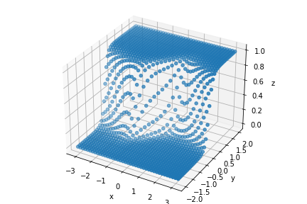
The last experiment presented in this work regards a classification problem. In this numerical test we generated a dataset in in the following way: We considered , if a point is such that , then , otherwise (see Figure 12(a)). As a 2D visual inspection, we depict a point with in red, while points with are coloured in blue (see Figure 12(b)).



Training the neural network
| (23) |
(where is a sigmoid activation for any ) for iterations with the Adam algorithm we reached a loss . The output of the neural network is the probability of a point being red. As a first example we want to find the points which are red with a probability higher than . To this end, we look for a point whose probability to be red is almost . We chose the point , which is red with a probability of . Then we passed as input to Algorithm 4 with and . In this way we are considering the interval as the output of the neural network – Remember that we cannot overpass , so . The resulting set is shown in Figure 13(a). The result of the algorithm is indeed a good approximation of the region of the red points, except for the white area between and in the upper part of the plots. To understand why the algorithm does not cover this area, let us zoom around the point , looking at the foliation in , see Figure 13(c). To separate the curves of the foliation more, we run the algorithm with . Algorithm 4 is building the blue region as follows. First it builds the equivalence class – the lowest light blue curve – of – the cyan dot in the picture – using the SiMEC algorithm. Then it moves away from the point along the red curve, to change equivalence class, using SiMExp. Let us denote with this new point. At this point we repeat the procedure, obtaining the plot above. Once we arrive at the point in which the red curve hits the boundary , we see that the right part equivalence class is convex and is lowering towards the bottom of the plot. To find the equivalence classes – namely the curves of the foliation – in the white area, we need to continue the procedure just described for a few points on the red curve in the region above .
|
|


Indeed, running again Algorithm 4 with up to yields the set in Figure 14(a). To space the curves of the foliation, we chose , see Figure 14(c). Zooming around the point we can see that all the equivalence classes covering the white area are passing trough points of the red curve produced by SiMExp with . Another way to solve this problem without continuing to run the the algorithm above would be try considering different starting point in the same equivalence class of .
|
|


As a final application, we build the separating hypersurface – in this case a line – between red and blue points. To this end, we run Algorithm 4 starting from a point which is red with a probability of approximatively . In this experiment we build the separating surface starting from , whose output is and we find all the points which are red with probability with . The separating surface produced by the algorithm, see Figure 14(b), is a curve approximating , as one expects.
6 Conclusions
In this work, starting from the geometric framework introduced in [22], we propose two algorithms: first we studied the SiMEC algorithm, which builds an approximation of the equivalence classes of neural network – solving the problem of finding the preimage of a point in the output manifold – presenting both the underlying theory and some numerical experiments. Then, before tackling the case of the preimage of a real interval, we discussed how to explore the input manifold changing equivalence classes with the SiMExp algorithm. At last we studied how to build the preimage of an interval using both SiMEC and SiMExp, including an application to a binary classifier. We showed that once a neural network is properly trained, the equivalence classes are well reconstructed, as well as families of equivalence classes. We applied the proposed method to a thermodynamics problem and to a classification task, showing that one can easily reconstruct the separating surface.
Future work will involve the extension of the SiMEC and SiMExp algorithms to the case of a neural network from to for . Moreover, further developments will be done for convolutional neural network and also frameworks that encompass also non smooth activation function.
The possible applications of the presented approaches are vary: on one hand one can employ the SiMEC algorithm to explore the class of equivalence of a point , and this exploration actually means that new synthetic data can be generated. On the other hand, the coupled role of the two prosed algorithms can provide useful insights on the behaviour of some class of neural networks, for example image classifiers that suffer from small perturbation on the input manifold, providing completely unreliable results. A further possible application is in medical imaging: for example, this exploration of the equivalence classes may give some indication on how much diagnostic images can be overexposed (or underexposed) without affecting the classification result.
References
- [1]
R. Liu, B. Sisman, Y. Lin, H. Li,
Fasttalker:
A neural text-to-speech architecture with shallow and group autoregression,
Neural Networks 141 (2021) 306–314.
doi:https://doi.org/10.1016/j.neunet.2021.04.016.
URL https://www.sciencedirect.com/science/article/pii/S0893608021001532 - [2] N. Carlini, D. Wagner, Audio adversarial examples: Targeted attacks on speech-to-text, in: 2018 IEEE Security and Privacy Workshops (SPW), 2018, pp. 1–7. doi:10.1109/SPW.2018.00009.
- [3] Q. Zhu, B. Du, P. Yan, Boundary-weighted domain adaptive neural network for prostate MR image segmentation, IEEE Transactions on Medical Imaging 39 (3) (2020) 753–763. doi:10.1109/TMI.2019.2935018.
- [4]
M. Gridach,
Pydinet:
Pyramid dilated network for medical image segmentation, Neural Networks 140
(2021) 274–281.
doi:https://doi.org/10.1016/j.neunet.2021.03.023.
URL https://www.sciencedirect.com/science/article/pii/S0893608021001118 - [5]
K. Chumachenko, A. Iosifidis, M. Gabbouj,
Feedforward
neural networks initialization based on discriminant learning, Neural
Networks 146 (2022) 220–229.
doi:https://doi.org/10.1016/j.neunet.2021.11.020.
URL https://www.sciencedirect.com/science/article/pii/S0893608021004482 - [6]
Z. Lyu, Y. Dong, C. Huo, W. Ren,
Deep match to
rank model for personalized click-through rate prediction, Proceedings of
the AAAI Conference on Artificial Intelligence 34 (01) (2020) 156–163.
doi:10.1609/aaai.v34i01.5346.
URL https://ojs.aaai.org/index.php/AAAI/article/view/5346 - [7] A. Effland, E. Kobler, T. Pock, M. Rajkovic̀, M. Rumpf, Image morphing in deep feature spaces: Theory and applications, J Math Imaging Vis 63 (2021) 309–327. doi:https://doi.org/10.1007/s10851-020-00974-5.
- [8]
M. Y. Seker, A. Ahmetoglu, Y. Nagai, M. Asada, E. Oztop, E. Ugur,
Imitation
and mirror systems in robots through deep modality blending networks, Neural
Networks 146 (2022) 22–35.
doi:https://doi.org/10.1016/j.neunet.2021.11.004.
URL https://www.sciencedirect.com/science/article/pii/S0893608021004329 - [9] M. Raissi, P. Perdikaris, G. Karniadakis, Physics-informed neural networks: A deep learning framework for solving forward and inverse problems involving nonlinear partial differential equations, Journal of Computational Physics 378 (2019) 686–707. doi:https://doi.org/10.1016/j.jcp.2018.10.045.
- [10]
S. S. Blakseth, A. Rasheed, T. Kvamsdal, O. San,
Deep
neural network enabled corrective source term approach to hybrid analysis and
modeling, Neural Networks 146 (2022) 181–199.
doi:https://doi.org/10.1016/j.neunet.2021.11.021.
URL https://www.sciencedirect.com/science/article/pii/S0893608021004494 - [11] C. Han, H. Hayashi, L. Rundo, R. Araki, W. Shimoda, S. Muramatsu, Y. Furukawa, G. Mauri, H. Nakayama, GAN–based synthetic brain MR image generation, in: 2018 IEEE 15th International Symposium on Biomedical Imaging (ISBI 2018), 2018, pp. 734–738. doi:10.1109/ISBI.2018.8363678.
- [12]
J. Sun, G. Zhong, Y. Chen, Y. Liu, T. Li, K. Huang,
Generative
adversarial networks with mixture of t-distributions noise for diverse image
generation, Neural Networks 122 (2020) 374–381.
doi:https://doi.org/10.1016/j.neunet.2019.11.003.
URL https://www.sciencedirect.com/science/article/pii/S0893608019303429 - [13] A. Creswell, T. White, V. Dumoulin, K. Arulkumaran, B. Sengupta, A. A. Bharath, Generative adversarial networks: An overview, IEEE Signal Processing Magazine 35 (1) (2018) 53–65. doi:10.1109/MSP.2017.2765202.
- [14] N. Ibtehaz, M. S. Rahman, Multiresunet : Rethinking the U-net architecture for multimodal biomedical image segmentation, Neural Networks 121 (2020) 74–87. doi:https://doi.org/10.1016/j.neunet.2019.08.025.
- [15] I. Melekhov, J. Kannala, E. Rahtu, Siamese network features for image matching, in: 2016 23rd International Conference on Pattern Recognition (ICPR), 2016, pp. 378–383. doi:10.1109/ICPR.2016.7899663.
- [16]
M. Henaff, J. Bruna, Y. LeCun, Deep
convolutional networks on graph-structured data, CoRR abs/1506.05163 (2015).
arXiv:1506.05163.
URL http://arxiv.org/abs/1506.05163 - [17] M. M. Bronstein, J. Bruna, Y. LeCun, A. Szlam, P. Vandergheynst, Geometric deep learning: Going beyond euclidean data, IEEE Signal Processing Magazine 34 (4) (2017) 18–42. doi:10.1109/MSP.2017.2693418.
- [18]
M. Hauser, A. Ray,
Principles
of Riemannian geometry in neural networks, in: I. Guyon, U. V. Luxburg,
S. Bengio, H. Wallach, R. Fergus, S. Vishwanathan, R. Garnett (Eds.),
Advances in Neural Information Processing Systems, Vol. 30, Curran
Associates, Inc., 2017.
URL https://proceedings.neurips.cc/paper/2017/file/0ebcc77dc72360d0eb8e9504c78d38bd-Paper.pdf - [19] F. Monti, D. Boscaini, J. Masci, E. Rodolà, J. Svoboda, M. M. Bronstein, Geometric deep learning on graphs and manifolds using mixture model CNNs, in: 2017 IEEE Conference on Computer Vision and Pattern Recognition (CVPR), 2017, pp. 5425–5434. doi:10.1109/CVPR.2017.576.
- [20] H. Shen, A differential topological view of challenges in learning with feedforward neural networks (2018). arXiv:1811.10304.
- [21] A. Gu, F. Sala, B. Gunel, C. Ré, Learning mixed-curvature representations in product spaces, in: ICLR, 2019.
- [22]
A. Benfenati, A. Marta, A singular
Riemannian geometry approach to Deep Neural Networks I.
Theoretical foundations, CoRR abs/2201.09656 (2022).
arXiv:2201.09656.
URL https://arxiv.org/abs/2201.09656 - [23] L. W. Tu, An Introduction to Manifolds, 2nd Edition, Springer-Verlag New York, 2011. doi:10.1007/978-1-4419-7400-6.
- [24] C. Xie, J. Wang, Z. Zhang, Z. Ren, A. L. Yuille, Mitigating adversarial effects through randomization., in: International Conference on Learning Representations, 2018.
- [25] M. do Carmo, Differential Geometry of Curves and Surfaces: Revised and Updated Second Edition, Dover Books on Mathematics, Dover Publications, 2016.
- [26] C. C. Aggarwal, Neural Networks and Deep Learning, Springer, Cham, 2018. doi:10.1007/978-3-319-94463-0.
- [27] I. Goodfellow, Y. Bengio, A. Courville, Deep Learning, MIT Press, 2016, http://www.deeplearningbook.org.
- [28] M. P. Deisenroth, A. A. Faisal, C. S. Ong, Mathematics for machine learning, Cambridge University Press, 2020.
- [29] V. Sitzmann, J. Martel, A. Bergman, D. Lindell, G. Wetzstein, Implicit neural representations with periodic activation functions, Advances in Neural Information Processing Systems 33 (2020) 7462–7473.
- [30]
I. Chraibi Kaadoud, A. Bennetot, B. Mawhin, V. Charisi, N. Díaz-Rodríguez,
Explaining
aha! moments in artificial agents through ike-xai: Implicit knowledge
extraction for explainable ai, Neural Networks 155 (2022) 95–118.
doi:https://doi.org/10.1016/j.neunet.2022.08.002.
URL https://www.sciencedirect.com/science/article/pii/S0893608022003021 - [31] Q. Nguyen, M. Hein, The loss surface of deep and wide neural networks, in: Proceedings of the 34th International Conference on Machine Learning - Volume 70, ICML’17, JMLR.org, 2017, p. 2603–2612.
- [32] H. Shen, Towards a mathematical understanding of the difficulty in learning with feedforward neural networks, in: Proceedings of the IEEE Conference on Computer Vision and Pattern Recognition (CVPR), 2018.
- [33] T. Kato, Perturbation Theory for Linear Operators, 1966.
- [34]
F. Rellich, J. Berkowitz,
Perturbation Theory of
Eigenvalue Problems, New York University. Institute of Mathematical
Sciences, Gordon and Breach, 1969.
URL https://books.google.it/books?id=NqeMQQ7US2MC