\pkgPyChEst: a Python package for the consistent retrospective estimation of distributional changes in piece-wise stationary time series
Abstract
We introduce \pkgPyChEst, a \proglangPython package which provides tools for the simultaneous estimation of multiple changepoints in the distribution of piece-wise stationary time series. The nonparametric algorithms implemented are provably consistent in a general framework: when the samples are generated by unknown piece-wise stationary processes. In this setting, samples may have long-range dependencies of arbitrary form and the finite-dimensional marginals of any (unknown) fixed size before and after the changepoints may be the same. The strength of the algorithms included in the package is in their ability to consistently detect the changes without imposing any assumptions beyond stationarity on the underlying process distributions. We illustrate this distinguishing feature by comparing the performance of the package against state-of-the-art models designed for a setting where the samples are independently and identically distributed.
Keywords: Changepoint estimation, time series, stationary ergodic, long-range dependence, consistency, \proglangPython
1 Introduction
Retrospective multiple changepoint estimation is a classical problem in statistics, with a vast literature concerning both parametric and nonparametric settings, (Basseville and Nikiforov 1993; Brodsky and Darkhovsky 1993; Müller and Siegmund 1994; Brodsky and Darkhovsky 2000; Csörgö and Horváth 1998) . The problem can be introduced as follows. A given sample
of length is formed as the concatenation of non-overlapping segments, where and . Each segment is generated by some unknown stochastic process. The process distributions of every pair of consecutive segments are different. The index where one segment ends and another starts is called a changepoint. The changepoints as well as the number of changes are unknown and the objective is to estimate them given the sample .
The changepoint estimation problem is usually considered in a framework where the samples in each segment are assumed to be independently and identically distributed (i.i.d.) and the changes are in the mean or in some fixed known moment, (Yao 1988; Carlstein 1988; Pan and Chen 2006; Lebarbier 2005; Harchaoui and Lévy-Leduc 2010; Ciuperca 2011; Chen et al. 2011; Fryzlewicz 2014). In the literature concerning methods for dependent time series the form of the change and the nature of dependence are usually restricted; for instance, the process distributions are assumed to have finite-memory or satisfy strong mixing conditions (Kokoszka and Leipus 1998; Lavielle 1999; Kokoszka and Leipus 2002; Davis et al. 2006; Hariz et al. 2007; Lavielle and Teyssiere 2007; Brodsky and Darkhovsky 2008; Brodsky and Darkhovsky 2013). Even if no restrictions are imposed on the memory of the processes, the finite-dimensional marginals before and after the changes are almost exclusively assumed to be different (Carlstein and Lele 1993; Giraitis et al. 1995). On the other hand, existing changepoint estimation packages are typically concerned with independent observations, where occasionally additional constraints such as parametric assumptions and moment conditions are placed on the distributions. In some cases the included methods are designed to detect changes in the mean or variance only, and the settings considered do not allow for consistency considerations of the estimators (Killick and Eckley 2014; Ross 2015; James and Matteson 2015; Truong et al. 2020)
We have implemented two consistent multiple changepoint estimators, proposed by Khaleghi and Ryabko 2012; Khaleghi and Ryabko 2014, which are designed to locate changes in the process distributions of highly dependent time series. The only assumption made is that each segment is generated by an (unknown) stationary ergodic process. In particular, no such assumptions as independence, finite memory or mixing are placed on the samples. Moreover, the marginal distributions of any fixed size before and after the change may be the same: the changes refer to those in the time-series process distributions. For example the mean, variance etc. may remain unchanged throughout the entire sequence. This means that the most general and perhaps the most natural notion of change is considered, that is, change in the distribution of the data. We also do not place any conditions on the densities of the marginal distributions (the densities may not exist). Since little assumptions are made on how the data are generated, this setting is especially suitable for highly dependent time-series, potentially accommodating a variety of new applications. To the best of our knowledge, \pkgPyChEst is the first software package to provide tools for the consistent estimation of distributional changes in time series with long-range dependencies.
The remainder of this paper is organized as follows. In Section 2 we give a mathematical formulation of the changepoint problem considered, and provide an overview of the methodology, as well as the possibilities and limitations of the framework that we consider. In Section 3 we introduce the \pkgPyChEst package, and describe how it can be installed and used, and provide some examples and use-cases of the package. In Section 4 we illustrate the robustness of our algorithms against long-range dependencies.
2 Methodology
In this section we briefly introduce the setting considered, and provide an overview of the algorithms included in \pkgPyChEst, as well as a discussion of our implementation. We refer to (Khaleghi and Ryabko 2012; Khaleghi and Ryabko 2014) for detailed arguments and technical proofs.
2.1 Problem formulation
In order to formalize the problem, we require some preliminary notation and basic definitions. Let be a measurable space corresponding to the alphabet. Here, could be a subset of or more generally a subset of equipped with its Borel -algebra. Let be the set of all -valued infinite sequences equipped with the Borel -algebra on generated by the cylinder sets. Stochastic processes are probability measures on . Associated with a process is a sequence of random variables with joint (process) distribution where for every , is the coordinate projection of an in element of onto its element. We call a process stationary if for all . For each and define the empirical measure of as
for and otherwise, where is the indicator function. A stationary process with corresponding sequence of random variables X is (stationary) ergodic if for every and it holds that This is equivalent to the standard definition involving the triviality of invariant measurable sets, see e.g. (Gray 2009).
The changepoint estimation problem considered in this paper can be formulated as follows. We are given a piece-wise stationary an -valued sample of length , formed as the concatenation of a number of stationary segments,
with changepoints at where each (stationary) segment is generated by one of unknown stationary ergodic processes . In Section 2 we described the changepoint problem, and informally stated that a piece-wise stationary sample is obtained as a concatenation of segments each generate by a stationary ergodic process. More formally, the process by which is obtained can be specified as follows. First, let be a measure on the space where, Define the infinite matrix of -valued random variables where are jointly distributed according to , so that for we have . For each , let and define the projection map which maps on its row. The marginal distribution of is then defined as the distribution induced by on the row of , i.e. . Next, define the mapping as where picks out the changepoint that is closest to from the left, with the convention that and . The piecewise stationary sample generated by with changepoints at can be specified as a sequence of coordinate projections such that for any and it holds that
It is straightforward to check that a set-function satisfying the above, extends to a probability measure on , with the property that the (marginal) distributions of the segments are each given by a stationary ergodic process distribution . Since it is assumed that , the indices are called changepoints. The consecutive segments are generated by different processes so that . However, their means, variances, or, more generally, their finite-dimensional marginal distributions may be the same upto some (unknown) fixed size. On the other hand, letting means that non-consecutive segments can have the same distribution. Observe that by this formulation, the finite-dimensional marginals of any fixed size before and after the changepoints may be the same. We consider a general notion, where the changes are in the process distributions. Our aim is to provide asymptotically consistent estimates of the unknown changepoints . An estimate is said to be asymptotically consistent if
| (1) |
We seek changepoint estimation algorithms that provide an asymptotically consistent estimate for every changepoint . Observe that the asymptotic regime simply means that the estimation error is arbitrarily small if the sequence is sufficiently long. That is, the problem is to retrospectively locate the changes and the given sample does not grow with time. This differs, for example, from the problem of online changepoint detection where the observations arrive sequentially over time, and the objective is to detect a change as soon as possible. Denote by
with , the minimum normalized length of the stationary segments, and let
In order for the consistency conditions of the algorithms implemented as part of this package to hold we require that . Note that this linearity condition is standard in the changepoint literature, although it may be unnecessary when simpler formulations of the problem are considered. Indeed, an equivalent assumption is made by Fryzlewicz 2014 for the simpler piece-wise i.i.d. setting. However, conditions of this kind are inevitable in the general setting that we consider, where there may be arbitrary long-range dependencies: if the length of one of the segments is constant or sub-linear in then asymptotic consistency is not possible in this setting.
2.2 A distance between process distributions
Most non-parametric approaches to estimating a changepoint are usually based on the following idea. Initially, every possible index is considered a potential changepoint. The difference between the empirical expectation of the two segments and on either side of every fixed is calculated, and the changepoint estimate is chosen as the index that maximizes this difference in absolute value. A more general approach is based on maximizing the difference between the empirical distributions of the two segments under a given norm. Different norms give rise to different test statistics. The commonly used distances include the Kolmogorov-Smirnov statistics, obtained when the difference is calculated under the norm, the Cramér-von Mises statistics corresponding to the use of norm, and the generalizations thereof. We rely on empirical estimates of a distributional distance between the underlying process measures to locate the changepoints. The distance between a pair of process distributions can be defined as
where, are positive summable real weights, and range over a countable field that generates the sigma-algebra of the underlying probability space. For a discrete alphabet range over the set of all possible tuples. For example, in the case of binary alphabets, the distributional distance is the weighted sum of the differences of the probability values (measured with respect to and ) of all possible tuples . For real-valued processes the sets range over the products of all intervals with rational endpoints (i.e. the intervals, all pairs of such intervals, triples, etc.). Asymptotically consistent estimates of this distance can be obtained by replacing unknown probabilities with the corresponding frequencies, provided that the corresponding process distributions are stationary ergodic. Although the distance involves infinite summations, the computational complexity of obtaining its empirical approximation is , see (Khaleghi et al. 2016) for a discussion. Our implementation of this distance relies on the Aho-Corasick Algorithm (Aho and Corasick 1975) for calculating empirical frequencies.
In principal, we can use any distance function between the samples, provided that the distance used reflects that between the underlying process distributions. In the case of changepoint analysis, the distance is required to satisfy convexity as well. It is important to note that the distinction between the underlying process distributions is not reflected by string metrics, such as the Hamming distance, or the Levenshtein distance, etc. The Hamming distance between two sequences is defined as the minimum number of substitutions required to transform one sequence into another, and the Levenshtein distance corresponds to the smallest number of deletions, insertions and substitutions needed to achieve the same objective, see e.g. (Stephen 1994). More generally, a string distance between a pair of sequences is if and only if the two sequences are exactly the same. However, what we require is for the distance to converge to for long enough samples, if and only if both sequences are generated by the same process distribution. Consider a simple example where the elements of the sequences and are drawn independently from a Bernoulli distribution with probability . Regardless of the value of , on average, the Hamming distance between the two sequences is while they are generated by the same process distribution. At the same time, the empirical estimate of the distributional distance between and becomes arbitrarily small for large enough .
2.3 Detecting the number of changepoints
In general, rates of convergence are provably impossible to obtain for stationary ergodic processes (Shields 1996). As a result, the two-sample test does not have a consistent solution in this framework (Ryabko 2010). This means that it is not possible to determine, even in the weakest asymptotic sense, whether or not two samples have been generated by the same or by different stationary ergodic distributions. An implication of this negative result is that it is provably impossible to determine the number of changes without making further assumptions. In light of this limitation, without placing any additional constraints on the underlying process distributions, in this software package we provide two options. With this theoretical impossibility result in mind, \pkgPyChEst provides two (consistent) algorithms as follows.
- •
The first algorithm is an implementation of the the so-called List-Estimator of Khaleghi and Ryabko 2012, which aims to produce a (sorted) list of candidate estimates whose first elements are consistent estimates of the true changepoints. More precisely, the algorithm generates an exhaustive list of possibly more than candidate estimates (but makes no attempt to estimate ). The produced list must have the property that its first elements are consistent estimates of the true changepoints. In order to achieve this goal, the list-estimator requires an additional parameter , which is a lower-bound on the minimum separation . It is worth noting that if the correct value of is known a-priori, it is then possible to consistently estimate the changepoints without any additional information, and in particular access to some would no longer be required (Khaleghi and Ryabko 2016).
- •
The second algorithm included in the package, is an implementation of the procedure proposed by Khaleghi and Ryabko 2014, which is able to consistently estimate the changepoints and detect the number of changes, provided that the total number of different process distributions is given. Note that in the specific case where all of the process distributions are different, knowing amounts to knowing the number of changepoints (). However, the required additional parameter can be in general very different from , and has a natural interpretation in many real-world applications. For instance, the sequence may correspond to the behavior of a system over time, which may have alternated times between a known number of states. In a simple case, the system may only take on states, for example, “normal” and “abnormal”. Another application of this setting would be in speech segmentation where the total number of speakers is known, while the number of alternations between the speakers is not available. Thus, the number of process distributions is provided as an intrinsic part of the problem, which is provably sufficient to estimate . See Section 2.4 for an informal overview of the algorithms as well as details concerning their implementation; more technical discussions can be found in the corresponding papers referenced above.
2.4 An overview of our implementations
In this section we give an overview of the changepoint estimation algorithms provided in the package focusing on our algorithmic implementations. Let us denote by the empirical estimate of the distributional distance ; we refer to (Khaleghi et al. 2016) for a definition and a discussion on computational considerations.
The following two operators namely, the intra-subsequence distance and the single-changepoint estimator are used in our methods. Let be a sample generated by a stochastic process and consider a subsequence of with .
- i.
Define the intra-subsequence distance of as
(2) - ii.
For some , define the single-changepoint-estimator of as
(3)
For simplicity of notation, from this point on we assume the floor and ceiling functions implicit.
2.4.1 List-Estimator
The changepoint estimation procedure proposed by Khaleghi and Ryabko 2012 works as follows. Given a piece-wise stationary sample and a lower-bound on the minimum (normalized) stationary segment length, a sequence of evenly-spaced indices is formed. The index-sequence partitions into consecutive segments of length . The intra-subsequence-distance is calculated in all but the first and last segments and is used as their performance scores. Next, an appropriate subset of the segments is selected through the following iterative procedure: initially, all but the first and last segment are marked as available, and at each iteration, an available segment of highest score is selected, and added to the final list. Noting that is a lower-bound on the minimum normalized distance between the changepoints, the available candidates within of the selected segment are made unavailable. The selection procedure continues until the set of available segments becomes empty. This is depicted below, where the downward arrows show the location of the indices.
Noting that the first and last segments are made unavailable at the outset, it is easy to see that by this procedure, the segments to the left and right of each available segment are made unavailable. The single-changepoint estimator is used to generate a candidate estimate within every selected segment. There may be more than candidate estimates produced; however, as shown by Khaleghi and Ryabko 2012 for long enough the first candidate estimates in the sorted list are consistent. We would like to point out that since the candidate estimates can be computed in parallel, our implementation of this algorithm is multi-threaded.
An informal argument as to why this procedure is consistent is as follows. When , the generated index-sequence partitions in such a way that every three consecutive segments of the partition contain at most one changepoint. Also, the segments are of lengths . Therefore, if is large enough, the single-changepoint-estimator produces consistent changepoint estimates within each of the segments that actually contains a true changepoint. Moreover, the performance scores of the segments without changepoints converge to , while each of those corresponding to the segments that contain a changepoint converge to a non-zero constant. Thus, the candidate estimates of highest performance score that are at least at a distance from one another, each consistently estimate a unique changepoint. We refer to the above reference for a rigorous proof of consistency.
2.4.2 Changepoint Estimator
The function called Changepoint Estimator in our package is an implementation of the algorithm proposed by Khaleghi and Ryabko 2014. Given a piece-wise stationary sample , a lower-bound on the minimum (normalized) stationary segment length, and the total number of different process distributions , the algorithm works as follows. First, the List-Estimator described is used to obtain an initial set of changepoint candidates. The estimates are sorted in increasing order appearance to give . The sorted changepoint estimates are in turn used to produce a set
of at most consecutive non-overlapping segments of , which are of possibly different lengths. The identified segments of are depicted below.
Next, a procedure based on time-series clustering is employed to remove redundant estimates. This is where the total number of process distributions is used. To this end, first a total of cluster centers are obtained as follows. The first segment is chosen as the first cluster center. Iterating over a segment is chosen as a cluster center if it has the highest minimum distance from the previously chosen cluster centers. Once the cluster centers are specified, the remaining segments are assigned to the closest cluster. As shown by Khaleghi and Ryabko 2014, for a long enough , this clustering algorithm will put the segments together if and only if they have the same (unknown) process distribution. In each cluster, the changepoint candidate that joins a pair of consecutive segments of is naturally identified as redundant and is removed from the list. This step of the algorithm is pictured below where denotes the cluster, .
In the above example, and each separate segments that, as identified by the clustering sub-routine, are generate by the same unknown process, and are thus considered as redundant. Once all of the redundant candidates are removed, the algorithm outputs the remaining candidate estimates.
An intuitive argument concerning the consistency of this procedure is as follows. First, note that for a long enough the List-Estimator produces an initial set of at least estimates whose first elements each uniquely and consistently estimate one of the changepoints. (Since is unknown, the fact that the correct estimates are located first in the list is irrelevant: what matters is that the correct changepoint estimates are somewhere in the list.) Therefore, if is long enough, the largest portion of each segment in is generated by a single process distribution. Since the List-Estimator ensures that the initial changepoint candidates are at least apart, the lengths of the segments in are linear in . Thus, it can be shown that for large enough , the empirical estimate of the distributional distance between a pair of segments in converges to if and only if the same process distribution generates most of the two segments. Given the total number of process distributions, for long enough the clustering algorithm groups together those and only those segments in that are generated by the same process. This lets the algorithm identify and remove the redundant candidates. As a result of the consistency of the List-Estimator, the remaining candidates are consistent estimates of the true changepoints. The proof can be found in (Khaleghi and Ryabko 2014).
3 Installation and Use
In this section we outline how to install and use \pkgPyChEst.
3.1 Installing \pkgPyChEst
The easiest way to install the \codePython package is to use \codePythons package-management system \codepip, which can be achieved by typing the following segment into a command line of their choice: {CodeInput} pip install PyChest
3.2 Using \pkgPyChEst
The \pkgPyChEst package provides two main functions, namely
- 1.
\code
list_estimator
- 2.
\code
find_changepoints
both described in the previous section. The \codelist_estimator takes a sample and a parameter \codemin_distance corresponding to a lower bound on the minimum normalized distance between the changepoints. Note that this parameter is denoted by in the mathematical descriptions given in Sections 2.3 and 2.4. The function can be called as follows. {CodeInput} >>> estimates = PyChest.list_estimator(seq, min_distance) The function \codefind_changepoints requires the same parameters as well as an additional integer corresponding to the total number of processes that generate the data; it can be called as described below. {CodeInput} >>> estimates = PyChest.find_changepoints(seq, min_distance, process_count) Next, we demonstrate how the package can be used. To this end, first we load the required packages as follows. {CodeInput} >>> import PyChest >>> import numpy as np We also fix a random seed for reproducibility. {CodeInput} >>> np.random.seed(1) We generate a piece-wise i.i.d. Bernoulli sample with changepoints at 2000 and 6500, where the parameter corresponding to the first and last segments is and that of the middle segment , i.e. {CodeInput} >>> seq = [] >>> seq.append(np.random.binomial(1, p=0.2, size=2000)) >>> seq.append(np.random.binomial(1, p=0.7, size=4500)) >>> seq.append(np.random.binomial(1, p=0.2, size=1500)) >>> seq = np.concatenate(sequence) Notice that the data so-generated is a piece-wise i.i.d. sample with changepoints at and , with the minimum length of the stationary segment equal to . There are a total two processes present, since the first and last segments have been generated by the same process. We can now execute \pkgPyChest to find the changepoints. Both the \codelist_estimator and \codefind_changepoints a lower bound on the minimum normalized distance between changepoint. The shortest stationary segment in this example is of length , and given that the sequence is of length , the minimum normalized stationary segment length equals . We assume this value unknown, and arbitrarily provide a parameter as input. {CodeInput} >>> min_distance = 0.125 >>> estimates = PyChest.list_estimator(seq, min_distance) The \codelist_estimator returns a \codePython of changepoint estimates at least apart, which are ordered in decreasing sequence of their performance scores as given by (2). As previously discussed, the theoretical consistency results guarantee that for a long enough sequence, with probability one, the first estimates in the list are arbitrarily close to the true changepoints. {CodeInput} >>> print(estimates) {CodeOutput} [1997, 6502, 4572] As can be seen above, the first two elements of the array returned by \codelist_estimator are good estimates of the true changepoints and in our example.
In addition to \codeseq and \codemin_distance, the \codefind_changepoints function also requires the total number of different processes that generate the data. Since there are three segments in our example with the first and last segments generated by the same process, the total number of processes here is . We refer to this parameter as \codeprocess_count and note that it has been mathematically denoted by in Section 2.4. {CodeInput} >>> process_count = 2 >>> estimates = PyChest.find_changepoints(seq, min_distance, process_count) {CodeInput} >>> print(estimates) {CodeOutput} [1997, 6502]
Next, we generate a real-valued sequence from the above binary-valued sequence by calculating its running mean (of window size ) as follows. {CodeInput} >>> N = 25 >>> seq = np.convolve(seq, np.ones(N)/N, mode=’valid’) Applying \codelist_estimator and \codefind_changepoints to the generated data we obtain the following results. {CodeInput} >>> min_distance = 0.125 >>> estimates = PyChest.list_estimator(seq, min_distance) {CodeInput} >>> print(estimates) {CodeOutput} [1989, 6489, 4582]
>>> process_count = 2 >>> estimates = PyChest.find_changepoints(seq, min_distance, process_count) {CodeInput} >>> print(estimates) {CodeOutput} [1989, 6489] The result is visualized in Figure 1.
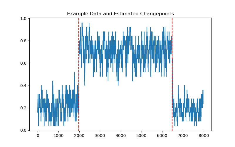
Observe that while the illustration in this example refers to the estimation of changes in the mean, the algorithms are more generally designed to detect changes in the distribution. This is shown in the next section.
4 Robustness against long-range dependencies
The strength of \pkgPyChEst is in its ability to consistently estimate changepoints in the presence of long-range dependencies. In this section we showcase this feature by comparing \pkgPyChEst to the state of the art algorithm Wild Binary Segmentation (WBS) proposed by Fryzlewicz 2014 which is provably consistent in the piece-wise i.i.d. setting; we rely on the implementation provided by the CRAN package \pkgwbs of Baranowski and Fryzlewicz 2019.
4.1 Stationary samples which possess long-range dependencies
As part of the experiments outlined in Section 4.2 we obtain the stationary segments of some of our piece-wise stationary samples as sample-paths of a subclass of stationary ergodic processes that do not belong to any “simpler” class. More specifically, we consider Irrational Rotations outlined below, which are classical examples of a stationary ergodic process that is not a -process, and that cannot be modelled by a hidden Markov model with a finite or countably infinite set of states, see, e.g. (Shields 1996).
4.1.1 Irrational Rotation
For a fixed , a binary-valued sample is generated from an Irrational Rotation as follows. First, we fix a parameter . Then, we sample uniformly at random from , and for each we obtain by shifting by to the right and removing the integer part, i.e.
The sequence is obtained from by thresholding at i.e., for each we set
| (4) |
It is well-known that if is irrational then forms a binary-valued stationary ergodic sample, that possesses long-range dependencies: it is not even mixing in the ergodic-theoretic sense (Shields 1996). We simulate by a floating point number with a long mantissa.
4.1.2 Hidden Irrational Rotation
In order to obtain a sample from a real-valued stationary ergodic process that is not mixing, we generate what we call a “Hidden Irrational Rotation”. To this end, we first simulate an irrational number by a floating point number with a long mantissa, and generate a binary-valued Irrational Rotation sample given by (4). Next, we draw two independent samples and , each generated uniformly i.i.d. from and respectively. We obtain as
| (5) |
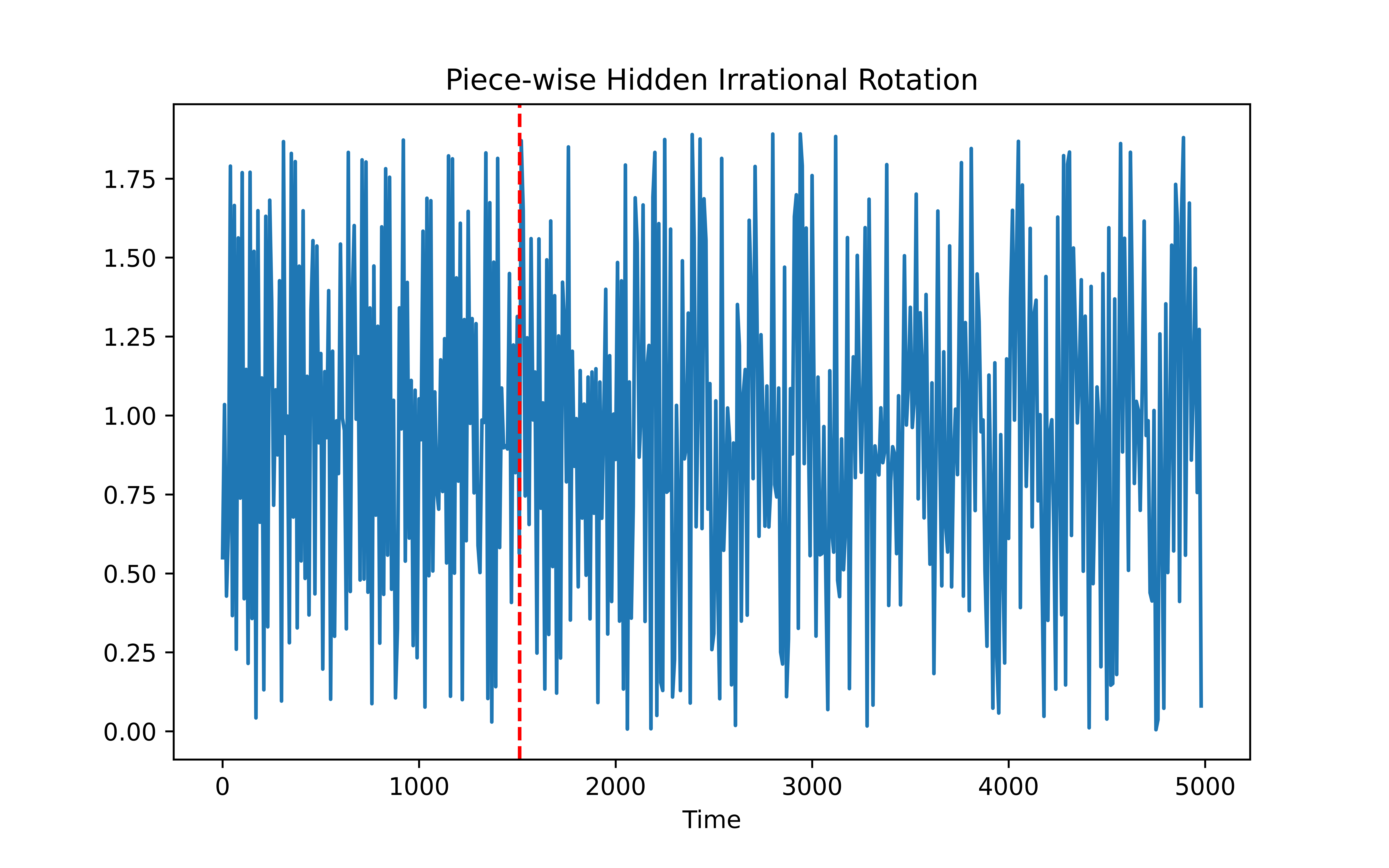
This forms a real-valued (non-mixing) stationary ergodic sample . Observe that if we deterministically set and for all we recover the binary-valued sample . Figure 2 illustrates an example of a piece-wise stationary sample, with a changepoint at such that the segments before and after it correspond to sample-paths of two different Hidden Irrational Rotations with parameters 11 1 and 22 2 respectively. Observe that while there is a change in the process distributions, it cannot be located visually and without appropriate statistical tools.
4.2 Illustrations
In this section we compare the performance of \pkgPyChEst against that of \pkgwbs. As mentioned previously, the latter provides a consistent changepoint estimation method for the case where the samples are piece-wise i.i.d. .
To calculate the performance of the algorithms, we rely on their estimation errors calculated as follows. Suppose that there are a total of changepoints in a sample of length . We calculate the estimation error of an algorithm that produces a total of candidate estimates as
| (6) |
In our first experiment we examine the convergence of the estimation error as sample-length increases. First, we consider the problem of locating a single change in distribution so that . We start with a simple setting where we generate piece-wise i.i.d. samples of length , each with a changepoint at ; the samples before the changepoint are generated i.i.d. according to a Bernoulli distribution with parameter and independently, those after the changepoint are generated i.i.d. according to a Bernoulli distribution with parameter . We set and provide \codefind_changepoints with \codemin_distance=0.21, and \codeprocess_count=2. We provide \pkgwbs with an upper-bound of on the number of changepoints together with the Strengthened Schwarz Information Criterion (SIC) penalty term as recommended by Baranowski and Fryzlewicz 2019. As can be seen in Figure 2(Left), the mean estimation error calculated by (6) (averaged over iterations) converges to for both algorithms. Next we repeated the same experiment, but this time we let and generated Hidden Irrational Rotations with shift parameters and before and after the changepoint respectively. To run the algorithms, we pass \codemin_distance=0.21, and \codeprocess_count=2 to \codefind_changepoints, and provided \pkgwbs with the same parameters as in the previous case, namely an upper-bound of on the number of changepoints and the Strengthened SIC penalty term. As shown in Figure 2 (Right), the mean error rate (calculated over iterations) of \pkgPyChEst approaches with increased sample length , while that of \pkgwbs remains consistently high. This experiment shows that the rate of convergence of for an algorithm such as \pkgwbs with consistency guarantees for the piece-wise i.i.d. setting can be better than that of \pkgPyChEst’s when the i.i.d. assumption holds. However, \pkgPyChEst is robust against long-range dependencies, and performs well on both piece-wise i.i.d. samples as well as piece-wise stationary samples.


In our second experiment, we consider the problem of locating changepoints in piece-wise stationary samples of length . First, we generate piece-wise i.i.d. Bernoulli samples with changepoints at and , so that . The three stationary segments are drawn independently where the first and last segments are generated i.i.d. according to a Bernoulli distribution with parameter and the middle segment is generated i.i.d. according to a Bernoulli distribution with parameter , leading to as the total number of process distributions. We pass \codeprocess_count=2 and \codemin_distance=0.21 to \pkgPyChEst’s \codefind_changepoints. We run \pkgwbs with an upper-bound of on together with the Strengthened SIC penalty term. Next, we consider the same problem, with the difference that the changepoints are located at and and the samples are piece-wise stationary ergodic processes with long-range dependencies. More specifically, the first and last segments are identically generated by a Hidden Irrational Rotation with shift parameter and the middle segment is generated by a different Hidden Irrational Rotation with as its shift parameter. We run both algorithms with the same input parameters as those provided in the piece-wise i.i.d. case above. The average (over iterations) errors (6) is reported in Table 1. Both algorithms perform well in the piece-wise i.i.d. setting. However, in the case of piece-wise Hidden Irrational Rotations \pkgwbs is unable to provide a single changepoint estimate, while \pkgPyChEst continues to perform well. As a result, this experiment serves as another demonstration of the robustness of \pkgPyChEst against long-range dependencies.
| piece-wise i.i.d. vs. piece-wise stationary process with long-range dependencies | ||
|---|---|---|
| \pkg PyChest | \pkg wbs | |
| (piece-wise i.i.d. ) Bernoulli | 0.000151 | 0.000124 |
| (piece-wise) Hidden Irrational Rotation | 0.000143 | 1 |
References
- Aho and Corasick (1975) Aho AV, Corasick MJ (1975). “Efficient string matching: an aid to bibliographic search.” Communications of the ACM, 18(6), 333–340.
- Baranowski and Fryzlewicz (2019) Baranowski R, Fryzlewicz P (2019). wbs: Wild Binary Segmentation for Multiple Change-Point Detection. R package version 1.4.
- Basseville and Nikiforov (1993) Basseville M, Nikiforov I (1993). Detection of abrupt changes: theory and application. Prentice Hall information and system sciences series. Prentice Hall.
- Brodsky and Darkhovsky (1993) Brodsky B, Darkhovsky B (1993). Non-parametric methods in change-point problems. Mathematics and its applications. Kluwer Academic Publishers.
- Brodsky and Darkhovsky (2000) Brodsky B, Darkhovsky B (2000). Non-parametric statistical diagnosis: problems and methods, volume 509. Kluwer Academic Pub.
- Brodsky and Darkhovsky (2008) Brodsky B, Darkhovsky B (2008). “Sequential change-point detection for mixing random sequences under composite hypotheses.” Statistical Inference for Stochastic Processes, 11(1), 35–54.
- Brodsky and Darkhovsky (2013) Brodsky B, Darkhovsky B (2013). “Asymptotically Optimal Methods of Early Change-Point Detection.” Sequential Analysis, 32(2), 158–181.
- Carlstein (1988) Carlstein E (1988). “Non-parametric Change-Point Estimation.” The Annals of Statistics, 16(1), 188–197.
- Carlstein and Lele (1993) Carlstein E, Lele S (1993). “Non-parametric change-point estimation for data from an ergodic sequence.” Teorya Veroyatnostei i ee Primeneniya, 38, 910–917.
- Chen et al. (2011) Chen Km, Cohen A, Sackrowitz H (2011). “Consistent multiple testing for change points.” Journal of multivariate analysis, 102(10), 1339–1343.
- Ciuperca (2011) Ciuperca G (2011). “A general criterion to determine the number of change-points.” Statistics & probability letters, 81(8), 1267–1275.
- Csörgö and Horváth (1998) Csörgö M, Horváth L (1998). Limit Theorems in Change-Point Analysis (Wiley Series in Probability & Statistics).
- Davis et al. (2006) Davis RA, Lee TCM, Rodriguez-Yam GA (2006). “Structural break estimation for nonstationary time series models.” Journal of the American Statistical Association, 101(473), 223–239.
- Fryzlewicz (2014) Fryzlewicz P (2014). “Wild binary segmentation for multiple change-point detection.” The Annals of Statistics, 42(6), 2243–2281.
- Giraitis et al. (1995) Giraitis L, Leipus R, Surgailis D (1995). “The change-point problem for dependent observations.” Journal of Statistical Planning and Inference, pp. 1–15.
- Gray (2009) Gray RM (2009). Probability, random processes, and ergodic properties, volume 1. Springer.
- Harchaoui and Lévy-Leduc (2010) Harchaoui Z, Lévy-Leduc C (2010). “Multiple change-point estimation with a total variation penalty.” Journal of the American Statistical Association, 105(492), 1480–1493.
- Hariz et al. (2007) Hariz S, Wylie J, Zhang Q (2007). “Optimal Rate of Convergence for Non-parametric Change-Point Estimators for Nonstationary Sequences.” Annals of Statistics, 35(4), 1802–1826.
- James and Matteson (2015) James N, Matteson D (2015). “ecp: An R Package for Nonparametric Multiple Change Point Analysis of Multivariate Data.” Journal of Statistical Software, Articles, 62(7), 1–25. ISSN 1548-7660.
- Khaleghi and Ryabko (2012) Khaleghi A, Ryabko D (2012). “Locating changes in highly dependent data with unknown number of change points.” In Advances in Neural Information Processing Systems, pp. 3086–3094.
- Khaleghi and Ryabko (2014) Khaleghi A, Ryabko D (2014). “Asymptotically consistent estimation of the number of change points in highly dependent time series.” In International Conference on Machine Learning, pp. 539–547.
- Khaleghi and Ryabko (2016) Khaleghi A, Ryabko D (2016). “Nonparametric multiple change point estimation in highly dependent time series.” Theoretical Computer Science, 620, 119–133.
- Khaleghi et al. (2016) Khaleghi A, Ryabko D, Mary J, Preux P (2016). “Consistent algorithms for clustering time series.” The Journal of Machine Learning Research, 17(1), 94–125.
- Killick and Eckley (2014) Killick R, Eckley I (2014). “changepoint: An R Package for Changepoint Analysis.” Journal of Statistical Software, 58(3), 1–19. ISSN 1548-7660.
- Kokoszka and Leipus (1998) Kokoszka P, Leipus R (1998). “Change-point in the mean of dependent observations.” Statistics & probability letters, 40(4), 385–393.
- Kokoszka and Leipus (2002) Kokoszka P, Leipus R (2002). “Detection and estimation of changes in regime.” Long-Range Dependence: Theory and Applications, pp. 325–337.
- Lavielle (1999) Lavielle M (1999). “Detection of multiple changes in a sequence of dependent variables.” Stochastic Processes and their Applications, 83(1), 79–102.
- Lavielle and Teyssiere (2007) Lavielle M, Teyssiere G (2007). “Adaptive detection of multiple change-points in asset price volatility.” In Long memory in economics, pp. 129–156. Springer.
- Lebarbier (2005) Lebarbier E (2005). “Detecting multiple change-points in the mean of Gaussian process by model selection.” Signal Processing, 85(4), 717 – 736.
- Müller and Siegmund (1994) Müller H, Siegmund D (1994). “Change-Point Problems.” Ims.
- Pan and Chen (2006) Pan J, Chen J (2006). “Application of modified information criterion to multiple change point problems.” Journal of multivariate analysis, 97(10), 2221–2241.
- Ross (2015) Ross G (2015). “Parametric and Nonparametric Sequential Change Detection in R: The cpm Package.” Journal of Statistical Software, Articles, 66(3), 1–20. ISSN 1548-7660.
- Ryabko (2010) Ryabko D (2010). “Discrimination between B-processes is impossible.” Journal of Theoretical Probability, 23(2), 565–575.
- Shields (1996) Shields P (1996). The Ergodic Theory of Discrete Sample Paths. AMS Bookstore.
- Stephen (1994) Stephen G (1994). String searching algorithms. World Scientific publishing company.
- Truong et al. (2020) Truong C, Oudre L, Vayatis N (2020). “Selective review of offline change point detection methods.” Signal Processing, 167, 107299.
- Yao (1988) Yao Y (1988). “Estimating the number of change-points via Schwarz’criterion.” Statistics & Probability Letters, 6(3), 181–189.