Dijkstra-Through-Time: Ahead of time hardware scheduling method for deterministic workloads
Abstract
Most of the previous works on data flow optimizations for Machine Learning hardware accelerators try to find algorithmic re-factorization such as loop-reordering and loop-tiling. However, the analysis and information they provide are still at very high level and one must further map them onto instructions that hardware can understand. This paper presents “Dijkstra-Through-Time” (DTT), an ahead of time compute and memory scheduling-mapping algorithm for deterministic workloads. It provides a simple implementation and supports accelerators with complex NoC configurations, at the expense of a long compilation process. This initial paper illustrates a proof of concept implementation to merge scheduling and data cache coherence mechanisms to get more optimized data flows.
Index Terms:
Machine Learning, Place and route, Accelerator, Tool chain, Data flow optimizationI Introduction
In recent years there has been a Cambrian explosion of hardware accelerators particularly related to area of Machine Learning(ML)[1]. One of the driving factors for this is the wide and ever-increasing application domain of machine learning, with each application imposing its unique size, cost, latency, accuracy, and power performance requirements. Additionally, the flexibility to support various or a select class of Neural Network(NN) models together with the ability to efficiently perform training along with inference are considered desirable [2]. Recent works such as nGraph[3], Glow[4] and TVM[5] aim to solve the issue of software compiler support for custom NN accelerators, while tools such as ZigZag[6], MAESTRO[7] and TimeLoop[8] implement complex hardware-aware data flow optimizations.
Most accelerators often rely on a multi-core architecture to perform computations in parallel. In many of these multi-core architectures, data movement follows a design philosophy similar to that of the original Stanford DASH processor[9]. DASH uses a cache coherence protocol that ensures the right copy of a page will always be used in the hardware, even if very little determinism can be assumed from the processing elements (called PEs henceforth).
In practice however, one might notice that the behavior of the PEs is in fact determined by the (known) program they execute. If the code sequence is deterministic (i.e. with no data dependent conditional codes present) one could try to read the programs of the PEs and create an optimized data flow that guarantees cache coherence without any classic hardware-implemented data consistency protocol.
A precedent for such a data flow can be found in the field of supply chain management which defines Pulled and Pushed flow[10]. In a pulled flow, the goods are only produced when ordered by a consummer, which is often preferred in practice because it scales well with uncertainty. On the other hand, in a pushed flow goods are produced before they are ordered and stored until purchase. Pushed flows create determinism in the supply chain, enabling economies of scale by producing or shipping the goods in bulk.
In the context of NN accelerator design, a typical implementation would be with PEs requesting data explicitly and receiving pages of data to work on i.e. with a pulled flow. In this paper, we investigate the pushed flow, where the PEs receive the data without explicitly requesting it. The idea stems from the fact that most NN workloads are deterministic in nature without conditional statements. Hence, this determinism can be exploited to pre-schedule workloads across PEs in an efficient way.
In this paper we are presenting “Dijkstra-Through-Time” (DTT) a python-based tool as a proof of feasibility of this idea. As the name indicates, DTT applies Dijkstra’s algorithm on a snapshot of system states taken at every instant. As these are our first results, we present the methodology with some qualitative analysis and leave quantitative comparison with practical NN models as future work.
The rest of the paper is organized as follows: In the first section, we present a high-level intuition of the DTT method, taking the implementation into account. The second section provides examples of using the algorithm to clarify the way DTT works, while in the final section we are going to present what a theoretical architecture leveraging the DTT algorithm would look like.
II Algorithm Overview
II-A Intuition of the Method
Before delving into the details of the DTT algorithm, we explain the logic behind this method on a trivial example described in the Fig. 1. The key idea behind DTT is that a data movement is the action of taking data in one place at some cycle and sending it to another place, where it will arrive at an ulterior cycle. Both the spatial (i.e. where the data is moving) and temporal (i.e. when the data is moving) components must be taken into account.
Let us consider in Fig. 1 that we are trying to perform a multiplication between two 8 bits operands A and B initially loaded in the SRAM at cycle 0. The interconnect between SRAM and register is 32 bits wide while the one between register and multiplier is 8 bits wide. Both interconnect buses have a latency of 1 clock cycle.
The proposed DTT algorithm would reach its solution in two steps. First, it notices that the only way to perform the multiplication is to send the operands A and B to the multiplier and that the first cycle where the required data can actually reach the PE is the cycle 3 (because of the bottleneck of “bus1”). We shall refer to this step in DTT as the placing step. Next, we use Dijkstra’s algorithm to find how to send both A and B to the PE at cycle 3. To do this, we are going to find a path on an abstract scheduling graph, shown in Fig. 2. In short, we are using Dijkstra’s algorithm to explore the different schedules and choose the best one where A and B reach the PE at cycle 3. We shall refer to this step as the routing step of the DTT method.
Dijkstra’s algorithm must route the operands one by one. The scheduling graph for the data movement of A is shown on the Fig. 2(a). The source node is shown in blue, the target node in orange, and the solution of the algorithm in green. Fig. 2(b) shows the scheduling graph when moving operand B. The link in red indicates that “bus1” is unavailable between the cycle 1 and 2, because it is already carrying the operand A which occupies all the available bandwidth (i.e. 8 bits).


In simple terms, the data movement schedule presented in Fig. 2(a) is
- 1.
First move A from SRAM to the register at cycle 0.
- 2.
Then move A from the register to the PE at cycle 1.
- 3.
Wait inside the PE until cycle 3.
Similarly, for Fig. 2(b), the movement of B is
- 1.
First move B from SRAM to the register at cycle 0.
- 2.
Then let B wait one cycle inside the register (as the 8 bit bus is busy moving A).
- 3.
Finally, move B from the register at cycle 2 and reach the PE at cycle 3.
II-B Data structures for the Algorithm
In this section, we briefly describe the data structures that were used to implement the DTT algorithm in our proof of concept Python code. The four main classes used for the implementation are the Datum class, the Node class, the Wire class and the Actor class.
The Datum class is used to represent a single unit of information (eg. a byte) in the algorithm. For instance in Fig. 1, A and B would each be a distinct Datum. In terms of code implementation, a Datum can be a simple integer.
The Node class represents some memory element in the physical hardware and is used to build the scheduling graph. In Fig. 1 “SRAM”, “Reg” and “PE” would be instances of the Node class. The Node class represents a node in the hardware layout and not a node in the scheduling graph, which contains an additional temporal information, as seen in Fig. 2. The history of the Node is implemented with a dictionary which yields for any clock cycle the list of Datum present in the Node.
The Wire class represents a path for data to move in the hardware layout. In the Fig. 1, “bus0” and “bus1” would be Wire instances. Note that not all Wire instances refer to physical wires. To let a Datum wait inside a Node, a pseudo waiting Wire is drawn, which is simply a Wire going from the Node to itself. The Node and Wire classes are used during the routing step of the DTT algorithm.
An Actor class is a dedicated class used in during the placing step describing some hardware element which can perform a specific action. For instance in Fig. 1, “PE” is an Actor which is able to perform a multiplication. The Actor class can also represent more complex hardware as described in section II-C.
II-C Placing Algorithm
The purpose of the placing step of DTT is to assign the operations to Actor instances such that it shall lead the routing step to find the best solution. But since the routing step is expensive, the placing step must rely on a simpler, less granular representation of the state of the hardware. This is analogous to the place and route algorithm used for FPGAs. Unlike for the routing step, which is done using Dijkstra’s algorithm, there is no single algorithm which can be used for the placing step of DTT. Heuristics can be used to obtain a better placement, which will lead to a better overall scheduling.
In this section, we are going to describe a simple placing algorithm, the First Best Fit algorithm. One requirement for this algorithm is to have some affinity function, which scores how fit an Actor is for some data. One possible affinity function would be to count the values in the input data already cached by the Actor. The high-level code for this First Best Fit placing is provided in Algorithm 1.
The exact condition on which an Actor becomes busy depends on the context. In this paper we will consider reconfigurable MAC arrays as PEs, which become busy when all their multipliers are in use for one or more dot products. The output of the placing step should be a succession of instructions holding at least 3 pieces of information: which list of Datum should be sent, where they should go (i.e. which Actor) and when they should arrive.
II-D Routing Algorithm
The core step of DTT is the routing algorithm, performed with Dijkstra’s algorithm applied on the scheduling graph. The output of the placing step gives information about what data should move, and the routing step finds how or through what to optimally move the data. The high-level pseudo-code for this routing step is given in Algorithm 2.
A part of this routing step is illustrated on the simple example of the Fig. 2. We can see that the operand A goes from “SRAM” at cycle 0 to “Reg” at cycle 1, and from there reaches “PE” at cycle 2, where it remains until cycle 3. As the algorithm 2 states, we would write this information in the associated Node and Wire instances. Thus, we can deduce that the operand B cannot go through “bus1” at cycle 1 (recall “bus 1” is busy moving A, Fig. 2(b)).
III Case Studies
III-A Step by Step Example

In this section, we are going to do a step by step run of DTT on a simple reproducible example, which can be used to test a DTT implementation. The hardware we are considering is described in Fig. 3. It contains a global DRAM, two input SRAM, four processing elements and one output SRAM. All the sizes, costs and delays of the elements of the hardware are given in the Table I.
| element_name | size | cost | delay |
|---|---|---|---|
| DRAM | 512B | ||
| SRAM_* | 64B | ||
| PE_*_input | 4B | ||
| PE_*_output | 2B | ||
| green bus | 16B | 10 | 4 |
| blue bus | 1B | 2 | 1 |
| wait wire | 1 |
The information in Table I is enough to build the scheduling graph for the routing step. The PEs also must be described for the placing step, with a simple black box model provided in Table II. Some of this information was estimated, and there might be more than one way to determine the right values to use. For instance, the Actor cool down, i.e. the delay in cycles that should be left between two sucessive operations, is usually determined through trial and error, as an underestimated value would lead to a timing fault in the routing step.
| Field | Value | Comment |
|---|---|---|
| Actor cooldown | 1 cycle | see algorithm 1 |
| multiplication delay | 1 cycle | after which the result is ready |
| distribution latency | 8 cycles | estimated time to fetch the operands |
| memory size | 4 bytes | size of the operand buffer |
| multiplier count | 2 | inferred from the memory size |
Before any computation is scheduled, the initial memory content must be described to DTT in order for it to know where each Datum can be found. This would be done by arbitrarily adding the Datum to the history of the DRAM Node (see the section II-B). In this example, we initially load the data numbered to in the DRAM. The workload used for the example is described in Table III(a), with an offset on the last operation to handle data dependency. Note that we consider dot products for our operations, that is because of the operations which can be sped up in ML computations involve some dot products. Examples of such operations include fully connected layers or convolutional neural networks.
| Operation | Result | Offset |
|---|---|---|
| + | ||
| + | ||
| + |
| Cycle | Node | Data |
|---|---|---|
| 8 | PE_0_input | [0, 1, 2, 3] |
| 8 | PE_1_input | [1, 2, 3, 4] |
| 8 | PE_2_input | [2, 3] |
| 8 | PE_2_input | [4, 5] |
| 28 | PE_0_input | [100, 101, 102, 103] |
Running the placing step for the provided workload yields the Table III(b). The PEs are assumed to be reconfigurable, hence several different dot products are scheduled together when multipliers are available. Before running the routing step, one must explain to DTT how the output values to will appear in the hardware, here by arbitrarily adding a Datum in the history of the appropriate Node instances (see the section II-B). This is similar to how Datum are loaded in the DRAM during the initialization. Once that has been taken care of, the routing step can be pursued, and its result is provided in Table IV.
| Datum | source Node | start cycle | end Node | end cycle |
|---|---|---|---|---|
| 0 | DRAM | 3 | SRAM_input_0 | 7 |
| 0 | SRAM_input_0 | 7 | PE_0_input | 8 |
| 1 | DRAM | 2 | SRAM_input_0 | 6 |
| 1 | SRAM_input_0 | 6 | PE_0_input | 7 |
| 2 | DRAM | 1 | SRAM_input_0 | 5 |
| 2 | SRAM_input_0 | 5 | PE_0_input | 6 |
| 3 | DRAM | 0 | SRAM_input_0 | 4 |
| 3 | SRAM_input_0 | 4 | PE_0_input | 5 |
| 1 | SRAM_input_0 | 7 | PE_1_input | 8 |
| 2 | SRAM_input_0 | 6 | PE_1_input | 7 |
| 3 | SRAM_input_0 | 5 | PE_1_input | 6 |
| 4 | DRAM | 0 | SRAM_input_0 | 4 |
| 4 | SRAM_input_0 | 4 | PE_0_input | 5 |
| 2 | DRAM | 3 | SRAM_input_1 | 7 |
| 2 | SRAM_input_1 | 7 | PE_2_input | 8 |
| 3 | DRAM | 2 | SRAM_input_1 | 6 |
| 3 | SRAM_input_1 | 6 | PE_2_input | 7 |
| 4 | DRAM | 1 | SRAM_input_1 | 5 |
| 4 | SRAM_input_1 | 5 | PE_2_input | 6 |
| 5 | DRAM | 0 | SRAM_input_1 | 4 |
| 5 | SRAM_input_1 | 4 | PE_2_input | 5 |
| 100 | PE_0_output | 21 | SRAM_output | 22 |
| 100 | SRAM_output | 22 | DRAM | 23 |
| 100 | DRAM | 23 | SRAM_input_0 | 27 |
| 100 | SRAM_input_0 | 27 | PE_0_input | 28 |
| 101 | PE_1_output | 20 | SRAM_output | 21 |
| 101 | SRAM_output | 21 | DRAM | 22 |
| 101 | DRAM | 22 | SRAM_input_0 | 26 |
| 101 | SRAM_input_0 | 26 | PE_0_input | 27 |
| 102 | PE_2_output | 19 | SRAM_output | 20 |
| 102 | SRAM_output | 20 | DRAM | 21 |
| 102 | DRAM | 21 | SRAM_input_0 | 25 |
| 102 | SRAM_input_0 | 25 | PE_0_input | 26 |
| 103 | PE_2_output | 18 | SRAM_output | 19 |
| 103 | SRAM_output | 19 | DRAM | 20 |
| 103 | DRAM | 20 | SRAM_input_0 | 24 |
| 103 | SRAM_input_0 | 24 | PE_0_input | 25 |
A deeper look into the Table IV reveals two important strengths of the DTT algorithm. First, DTT will spontaneously optimize the data movements for the operations. For instance, the red part of the Table IV shows that the Datum 1 was originally sent to the PE_0 for the first dot product, and DTT will fetch it from cache instead of DRAM for the second operation. Similarly, notice in blue that DTT will naturally use the Datum to to perform the last dot product. DTT treats these values in the same way it treats values coming from the DRAM. If neural network layers are represented as a sequence of dot products, DTT will thus be able to optimize data movement across more than one layer at a time unlike classic for-loop refactoring algorithms. Thus if weights are reused in a NN model, DTT will try to reuse them on chip as far as possible without reloading them from main memory. To enable this, the reused weights must be marked during workload description to DTT.
III-B Reduction Network
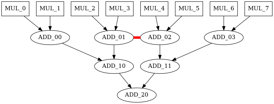
A reduction network is a set of interconnected adders which will accumulate the result of some multipliers. This is used to compute one or several dot products at the same time. Scheduling reductions with DTT is not immediately obvious, as the algorithm is naturally more suited for distributing values. In practice, one only needs to pretend to distribute the results to the multipliers and play the computed data flow backwards to schedule a reduction. This is because the addition and data reuse operation have an opposite data flow.
Most reduction networks take the form of a binary tree where the leaves are multipliers and the nodes are adders. One limitation of such a reduction network is that performing more than one dot product at a time on the network will lead to a lot of blocking. To improve on this design, the paper [11] proposed the “augmented reduction tree” recreated in Fig. 4, which is a binary tree with an additional connection between ADD_01 and ADD_02. Hypothetically, a hardware designer would want to benchmark the accelerator with and without the “augmented connection” to see if its benefits over weigh its costs. DTT can be used to create a prototyping back end for this purpose, which can be simply modified to compare the two reduction trees: simply remove from the description of the hardware graph the Wire between the Node instances ADD_01 and ADD_02 to benchmark the simple reduction tree, as shown in Fig. 5.

Some information that designers might find interesting and can be easily extracted from DTT are:
- 1.
The energy savings for a given workload with the augmented connection,
- 2.
The runtime difference between the normal and augmented reduction trees,
- 3.
The utilization rate of the augmented connection in the workload,
These low-level statistics would then be used to decide whether an augmented reduction tree or a simple reduction tree should be included in the designed hardware.
III-C Working with complex Hardware
For the last example, we are going to explain how a more complex hardware can be handled by DTT. This is meant to show the flexibility of the algorithm in more interesting cases. The hardware for this example is shown in Fig. 6. It uses a butterfly-style distribution network to send data from a global DRAM to several high-level components. In this design, seven ML accelerators are used (in blue along with a general-purpose processor (in green on the Fig 6). The idea here is that the NN model is made of several types of operations. Let us assume that only dot products, matrix multiplications and custom functions are used here. The dot products and matrix multiplications can be carried out by either the CPU or an accelerator, but an accelerator would be faster and more efficient. The rare custom functions however may only be performed out by the CPU.
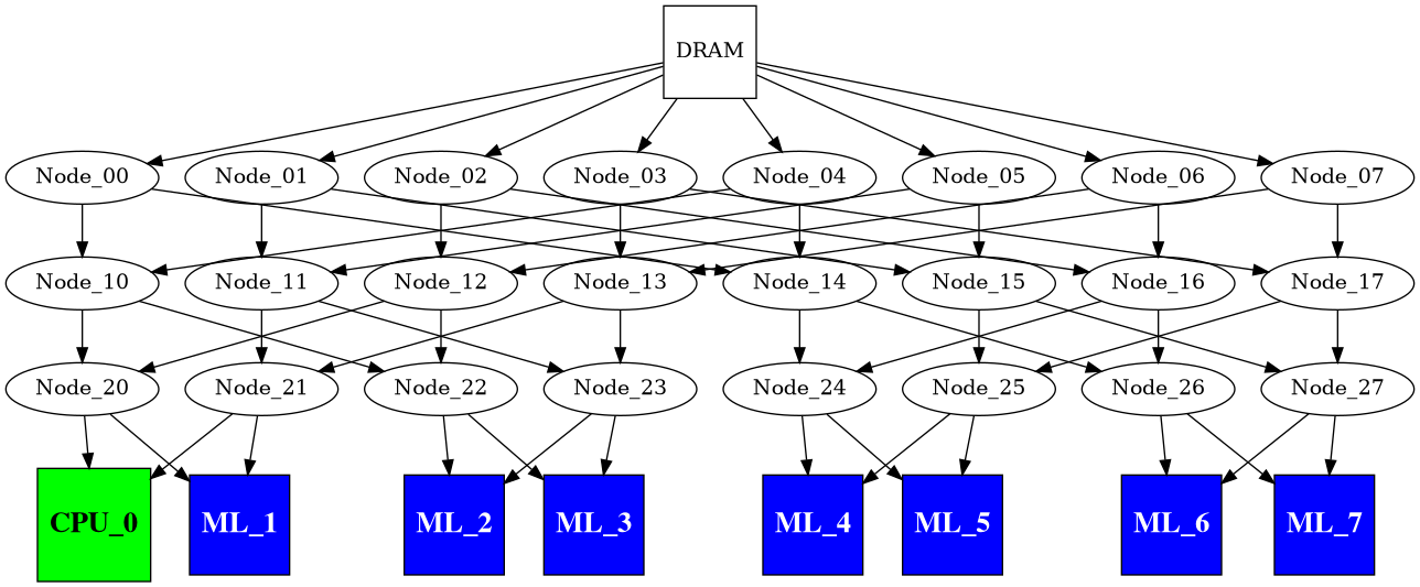
We are going to modify the placing step described in Algorithm 1. Since not every PE can carry out every operations, we first have to filter for the provided operation code the Actors which are relevant for the computation. The new placing step is presented in 3.
The routing step however would remain unchanged. This may come as a surprise, since several different operations are involved, but as mentioned before the only information considered for the routing step are: what data should be moved, where is it going to and when should it arrive. For as far as the routing algorithm is concerned, moving data for a dot product is no different than moving it for a custom computation. This also implies that DTT will spontaneously optimize data movements across different operations.
When benchmarking such hardware, a new issue might arise: the upstream DSE tool used probably does not understand what a butterfly network is. One would provide a simpler hardware description to optimize the workload for, and then take the optimized neural network and use DTT to schedule it for the complex hardware. For instance, the hardware of Fig. 6 could be described as Fig. 7 to a tool such as ZigZag or Timeloop.

Although giving an inaccurate description of the accelerator to the DSE tool could mean that its solution will be sub-optimal, it should still give a much better starting point for DTT.
IV DTT-based NoC
In this last part, we are going to present and end to end theoretical architecture that would take advantage of the DTT algorithm to optimize data movements in its NoC. In this architecture, the Datum considered will thus be entire memory pages.
IV-A Compiler overview
The compiler for the architecture would take as input a single threaded stream of operations to execute on the hardware. Its first task is to multi-thread those tasks between the various PEs in the architecture by running the placing step of the DTT algorithm. This approach is reminiscent of VLIW compilers[12], except that VLIW compilers also have to deal with runtime branches, while those do not appear in DTT’s deterministic workloads. As explained in section III-C, this placing step can accommodate heterogeneous PEs.
Once the placing step of DTT is over, the compiler knows when each operation should be performed and where they should take place. The routing step is used to decide how to send the data to the PEs so that they will be able to start their computations on time. The order in which data movement will happen in the NoC is:
- 1.
The controller asks a source Node to send a page to another PE
- 2.
The data movement takes place and the PE receives the page
- 3.
The controller sends the instruction to the PE and the computation starts
Because data arrives before the PEs start their operations, the PEs will never cache miss. In practice though, DTT has two weaknesses which prevent us from using it directly:
- •
The routing step is too expensive to be performed on an edge device,
- •
The output of the routing step (a list of data movements) is too big to be reasonably sent to an edge device.
Fortunately, there is a known solution to those issues, which is inspired by macro-routing[13]. The idea is to provide DTT with checkpoints that it can use to forget what came before. Hence, once the compiler is done performing the routing step, it only saves way-points (i.e. a few specific points the path has to traverse in order) from the paths instead of the whole path. Those way-points will be placed by the compiler into a binary file along with the scheduled operations for the accelerator.
IV-B DTT controller
Because we rely on DTT, the PEs used in our theoretical architecture do not use a distributed cache coherence protocol, but instead a global hardware controller connected to the NoC. This controller is here intended to be a small CPU core, although dedicated hardware might also be used. This controller has three main responsibilities:
- 1.
It reads the input program for the accelerator
- 2.
It reconstructs the paths for the data movements from the way-points
- 3.
It sends control packets to the PEs in order to have them realize the data movements it computed
The way points computed by the compiler and saved into the program file are sent to the hardware controller, which will run Dijkstra’s algorithm again to fill in the missing movements between the way-points at run-time. This technique could be seen as analogous to compressing a video to only its key-frames, then filling the intermediary frames via interpolation[14]. After the reconstruction of paths from the DTT algorithm, each data movement has to be turned into a control packet that will be sent by the controller to the relevant PEs.
The control packets would be sent over the NoC using dynamic routing protocols (as opposed to a fixed route decided by the controller) and should have plenty of time to reach their targets before the data movement needs to be carried out. To be sure that the control packets are consumed at the right time, a simple TTL (Time-toLive) mechanism could be used. Once the control packets are consumed, they will trigger a 2-way DMA access, sending the data from the source to the target (without going through the controller) and following the route decided by DTT. This ensures no unexpected congestions will appear in the NoC, as all the data movements have been foreseen by the controller.
IV-C Comparison with directory-based protocol
One significant asset of using DTT, compared to other coherent networking approaches, is its ability to optimize the data movements. Two possible traffic optimizations with DTT are shown in Fig. 8. During the routing step, DTT will use Dijkstra’s algorithm to find the shortest way to bring the required data to the PEs for the operations, leading to an expected improvement in the overall performance of the accelerator. This works because the cache coherence is ensured by one omniscient actor, hence finding correct optimizations becomes much easier.


The controller used in the theoretical architecture creates a bottleneck for the execution, as every operation needs to be processed by the controller before being executed in the chosen PE. Thus, a DTT based architecture is expected to not scale as well as a directory-based architecture, which is summarized in Table V.
| Protocol | Bus-snooping | DTT | Full-directory |
|---|---|---|---|
| Bottleneck | Bus bandwidth | Controller compute | Node distance |
| Best for | Small NoC | Medium NoC | Large NoC |
| Determinism | No | Required | No |
V Conclusion
In this paper we presented DTT, a low complexity ahead of time hardware scheduling method. We explained how the algorithm works and detailed important parts of its implementation. Several examples were shown to show how DTT can handle reconfigurable and custom hardware. Finally, we highlighted that DTT opens new opportunities for hardware designers by enabling them to quickly draft prototyping back ends. As mentioned at the beginning of the paper, DTT is currently a proof of concept. As future improvement we would like to show its usage with an application on a real ML workload.
References
- [1] A. Reuther, P. Michaleas, M. Jones, V. Gadepally, S. Samsi, and J. Kepner, “Survey and benchmarking of machine learning accelerators,” in IEEE High Performance Extreme Computing Conference, 2019.
- [2] V. Sze, Y.-H. Chen, T.-J. Yang, and J. S. Emer, Efficient Processing of Deep Neural Networks. Morgan & Claypool Publishers, 2020.
- [3] S. Cyphers, A. K. Bansal, A. Bhiwandiwalla, J. Bobba, M. Brookhart, A. Chakraborty, W. Constable, C. Convey, L. Cook, O. Kanawi, R. Kimball, J. Knight, N. Korovaiko, V. K. Vijay, Y. Lao, C. R. Lishka, J. Menon, J. Myers, S. A. Narayana, A. Procter, and T. J. Webb, “Intel nGraph: An Intermediate Representation, Compiler, and Executor for Deep Learning,” 2018. [Online]. Available: http://arxiv.org/abs/1801.08058
- [4] N. Rotem, J. Fix, S. Abdulrasool, S. Deng, R. Dzhabarov, J. Hegeman, R. Levenstein, B. Maher, N. Satish, J. Olesen, J. Park, A. Rakhov, and M. Smelyanskiy, “Glow: Graph lowering compiler techniques for neural networks,” 2018. [Online]. Available: http://arxiv.org/abs/1805.00907
- [5] T. Chen, T. Moreau, Z. Jiang, L. Zheng, E. Q. Yan, H. Shen, M. Cowan, L. Wang, Y. Hu, L. Ceze, C. Guestrin, and A. Krishnamurthy, “TVM: an automated end-to-end optimizing compiler for deep learning,” in USENIX Symposium on Operating Systems Design and Implementation, 2018.
- [6] L. Mei, P. Houshmand, V. Jain, J. S. P. Giraldo, and M. Verhelst, “Zigzag: A memory-centric rapid DNN accelerator design space exploration framework,” 2020. [Online]. Available: https://arxiv.org/abs/2007.11360
- [7] H. Kwon, P. Chatarasi, V. Sarkar, T. Krishna, M. Pellauer, and A. Parashar, “MAESTRO: A Data-Centric Approach to Understand Reuse, Performance, and Hardware Cost of DNN Mappings,” IEEE Micro, 2020.
- [8] A. Parashar, P. Raina, Y. S. Shao, Y. Chen, V. A. Ying, A. Mukkara, R. Venkatesan, B. Khailany, S. W. Keckler, and J. Emer, “Timeloop: A systematic approach to dnn accelerator evaluation,” in IEEE International Symposium on Performance Analysis of Systems and Software, 2019.
- [9] D. Lenoski, J. Laudon, K. Gharachorloo, W. . Weber, A. Gupta, J. Hennessy, M. Horowitz, and M. S. Lam, “The stanford dash multiprocessor,” Computer, vol. 25, no. 3, pp. 63–79, 1992.
- [10] D. Pyke and M. Cohen, “Push and pull in manufacturing and distribution systems,” Journal of Operations Management, vol. 9, p. 24–43, 01 1990.
- [11] H. Kwon, A. Samajdar, and T. Krishna, “MAERI: Enabling Flexible Dataflow Mapping over DNN Accelerators via Reconfigurable Interconnects,” in Architectural Support for Programming Languages and Operating Systems, 2018.
- [12] S. Jee and K. Palaniappan, “Dynamically scheduling vliw instructions with dependency information,” 02 2002, pp. 15 – 23.
- [13] S. Dragos and M. Collier, “Macro-routing: a new hierarchical routing protocol,” in IEEE Global Telecommunications Conference, 2004.
- [14] C.-Y. Wu, N. Singhal, and P. Krähenbühl, “Video compression through image interpolation,” 2018. [Online]. Available: https://arxiv.org/abs/1804.06919