02CCS: Applied computing Online shoppingCCS: Mathematics of computing Causal networksCCS: Computing methodologies Artificial intelligence

Lu Cheng¹, Ruocheng Guo², Huan Liu¹ Affiliation: ¹ School of Computing and Augmented Intelligence, Arizona State University, USA
² School of Data Science, City University of Hong Kong, China email: lcheng35, huanliu@asu.edu, ruocheng.guo@cityu.edu.hk

2022; © acmcopyright

Abstract.

Online reviews enable consumers to engage with companies and provide important feedback. Due to the complexity of the high-dimensional text, these reviews are often simplified as a single numerical score, e.g., ratings or sentiment scores. This work empirically examines the causal effects of user-generated online reviews on a granular level: we consider multiple aspects, e.g., the Food and Service of a restaurant. Understanding consumers’ opinions toward different aspects can help evaluate business performance in detail and strategize business operations effectively. Specifically, we aim to answer interventional questions such as What will the restaurant popularity be if the quality w.r.t. its aspect Service is increased by 10%? The defining challenge of causal inference with observational data is the presence of “confounder”, which might not be observed or measured, e.g., consumers’ preference to food type, rendering the estimated effects biased and high-variance. To address this challenge, we have recourse to the multi-modal proxies such as the consumer profile information and interactions between consumers and businesses. We show how to effectively leverage the rich information to identify and estimate causal effects of multiple aspects embedded in online reviews. Empirical evaluations on synthetic and real-world data corroborate the efficacy and shed light on the actionable insight of the proposed approach.

Keywords:

Online Reviews, Causal Effect Estimation, Hidden Confounder, Multi-Modality, Multi-Aspect Sentiment

1. Introduction

Online reviews have become a critical source to evaluate business performance, raising considerable research efforts to understanding the effects of online reviews. Due to the complexity of using the high-dimensional text in causal studies, these reviews are typically simplified as an overall numerical rating (Anderson and Magruder 2012) or an aggregated sentiment score (Wang et al. 2017). However, such coarse-grained analysis provides limited information about strategizing business operations partly because it often results in findings that are inconsistent or even conflict with each other (Li et al. 2019). Text in online reviews provides detailed information about consumers’ opinions toward different aspects of a business. For example, Fig. 1 depicts a Yelp review with an overall rating of 3-star. In this figure, a plain-text review expresses a positive opinion toward the aspect food and negative opinions toward aspect ambience and service. This granular-level analysis of the content in online reviews help evaluate business performance in different dimensions and strategize operations effectively. Therefore, we seek an aspect-level effects estimation, a fine-grained analysis of how consumers’ opinions (sentiments) toward different aspects of a business expressed in the reviews – multi-aspect sentiment (MAS) – influence business popularity.

Refer to caption — Figure 1. An example of Yelp reviews. Different aspects (e.g., Food) are highlighted in different colors. Best viewed in color.

Estimating causal effects of MAS on popularity is essentially to intervene on individual sentiment aspects and answer questions such as “What will the restaurant popularity be if the quality w.r.t. aspect Service is increased by 10%?’’¹¹ 1 We assume that consumers’ opinions toward an aspect reflect its quality. Interventions could be formally justified by controlling confounding bias -- the influence of variables that cause spurious correlations between treatment assignment²² 2 We use treatments and (potential) causes exchangeably. (e.g., MAS) and the outcome (e.g., popularity). In observational studies, confounders might be unobserved or unmeasured, or hidden confounders (HC), such as a consumer’s food preference. Common solution is either assuming away the presence of HC or using proxy variables (i.e., observed covariates) to approximate them (Louizos et al. 2017; Miao et al. 2018).

However, when applied to our problem, selecting the ‘right’ proxies is especially challenging due to the multi-modality of online review systems such as the consumers’ profile information, businesses’ attributes, and consumer-restaurant interactions (i.e., a consumer writes reviews for specific restaurants). First, existing proxy strategies might lead us to include covariates insufficient to adjust for confounding biases. Second, even with sufficiently rich covariate set, one may confront the obstacle of how to exclude ‘bad’ covariates, i.e., variables that induce bias when they are used as proxy variables. When estimating effects of online reviews on popularity, business revenue would be a ‘bad’ proxy because it is causally affected by the outcome (i.e., popularity). These methods and their challenges, however, suggest a new approach for causal effect estimation: we might have recourse to a representation of the multi-modal proxy variables observed in online review systems. The intuition is that the richer the covariate set is, the more likely it is to accurately predict the outcomes and estimate the effects (D’Amour et al. 2021). Previous findings (e.g., (Guo et al. 2020b)) also advocated to use network information such as social networks that embed the homophily effect to learn HC. Further, learning a representation of the multi-modal covariate set rather than directly using the covariate set itself can help block the undesired biases induced by bad covariates when they are conditioned on. Therefore, desired representations should contain sufficient information for confounding adjustment, exclude biases induced by bad proxy variables, and helps provide less biased and low-variance causal estimates. This work presents a method to simultaneously learn such representations and estimate causal effects of multi-aspect online reviews on popularity.

Contributions. We develop a principled framework–Deconfounded Multi-Modal Causal Effect Estimation (DMCEE) to estimate causal effects of MAS on business popularity in the presence of hidden confounding, with low bias and variance. DMCEE provides valid causal inferences through two primary components: (1) the Proxies Encoding Network that maps the multi-modal proxies to a shared latent space; and (2) the Causal Adjustment Network that seeks to extract information from the latent representation that is sufficient to adjust for the confounding while excluding undesired biases. At its core, DMCEE jointly recovers HC from observed multi-modal proxies and estimate effects of online reviews from different aspects.

The main contributions of this work are: (1) we study a novel and practical problem to examine the effects of multiple aspects of a business expressed in online reviews on business popularity in the presence of HC (Section 2); (2) we theoretically prove that the studied problem is causally identifiable (Appendix A) and propose an effective approach that aims to estimate causal effects and approximate HC by leveraging multi-modal proxies and appropriate causal adjustment (Section 3); (3) we validate the effectiveness of DMCEE using synthetic data and two novel datasets collected from the real world (Section 4). The case studies further illustrate how DMCEE can help business owners strategize business operations.

2. Problem Definition

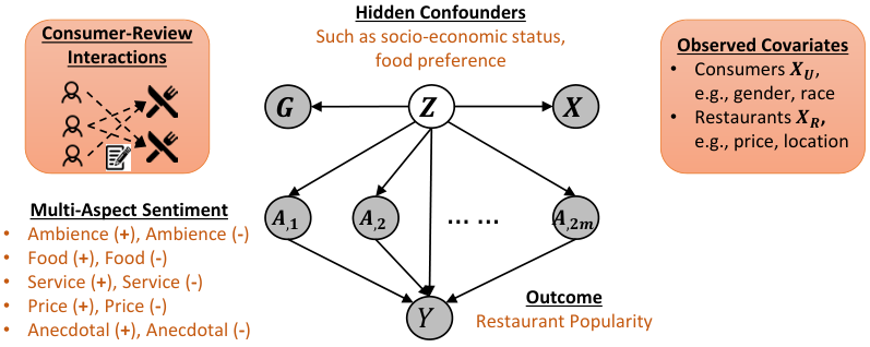
We first illustrate the problem using a causal graph described in Fig. 2. Given online reviews and restaurant popularity, our goal is to estimate the effects of MAS ( ${\bf A}$ ) on popularity ( $Y$ ) in the presence of shared HC ( ${\bf Z}$ ). We also observe rich covariates with multi-modalities, including consumers’ profile information ( ${\bf X}_{U}$ , e.g., race), restaurants’ attributes ( ${\bf X}_{R}$ , e.g., price range), and consumer-restaurant interactions ( ${\bf G}$ ) that further manifest the behavioral/operational similarity between consumers/restaurants (Wang et al. 2019).

We now formally define the proposed problem within the standard Potential Outcome framework (Rubin 2005). Given a set of $N_{R}$ restaurants $\mathcal{R}$ along with a corpus of online reviews $\mathcal{C}$ written by a group of $N_{U}$ consumers $\mathcal{U}$ , for each restaurant $r\in\{1,2,...,N_{R}\}$ , we extract $m$ aspects from $\mathcal{C}$ and each aspect is associated with continuous positive and negative sentiment scores. Previous findings showed that positive and negative online reviews exert different influences on the outcomes (Tsao et al. 2019). We denote the MAS for restaurant $r$ as a $2m$ -dimensional vector $\bm{a}_{r}=<a_{r1},a_{r2},...,a_{r2m}>$ . A potential outcome function then maps $\bm{a}_{r}$ to the outcome $y_{r}(\bm{a}_{r})$ , i.e., $y_{r}(\bm{a}_{r}):\mathbb{R}^{2m}\rightarrow\mathbb{R}.$ The fundamental problem in causal inference is that only one potential outcome can be observed (Guo et al. 2020a), e.g., $Y_{r}({\bf A}_{r})$ for a certain configuration of ${\bf A}_{r}$ . Let ${\bf X}_{R}$ and ${\bf X}_{U}$ represent restaurant and consumer covariates, respectively. Interactions between consumers and restaurants are defined as a bipartite graph $\mathcal{G}=(\mathcal{U},\mathcal{R},\mathcal{E})$ where nodes consist of consumers and restaurants, and edges set $\mathcal{E}$ denotes review-writing relationships. The adjacency matrix of $\mathcal{G}$ is ${\bf G}\in\mathbb{R}^{N_{R}\times N_{U}}$ where 1 denotes $u\in\mathcal{U}$ writes a review for $r\in\mathcal{R}$ , 0 otherwise.

We now define the problem as follows:

Definition 0 (Estimating Effects of Multi-Aspect Online Reviews).

Given the multi-modal information, we aim to study how sentiment aspects in ${\bf A}\in\mathcal{A}$ extracted from $\mathcal{C}$ influence the restaurant popularity $Y$ in the presence of HC ${\bf Z}$ . Specifically, we are interested in jointly estimating the average treatment effect (ATE) of individual sentiment aspect ${\bf A}_{,j},j\in\{1,2,..,2m\}$ on $Y$ :

(1)

\tau_{j}=\mathbb{E}[Y_{r}(a_{rj})]-\mathbb{E}[Y_{r}(a^{\prime}_{rj})]\quad r\in\{1,2,...,N_{R}\},

where $\mathbb{E}[Y_{r}(a_{rj})]$ denotes the expected restaurant popularity with aspect sentiment score $a_{rj}$ .

As the aspect sentiment scores are continuous and there are multiple aspects, this is essentially a continuous multiple treatment (dose) effect estimation problem. The estimation is unbiased iff $\mathbb{E}[Y_{r}(a_{rj})]=\mathbb{E}[Y_{r}(a_{rj})|A_{rj}=a_{rj}]$ , i.e., all confounding is properly adjusted for. HC can generate a statistical dependency between ${\bf A}$ and $Y$ , i.e., $\mathbb{E}[Y_{r}(a_{rj})]\neq\mathbb{E}[Y_{r}(a_{rj})|A_{rj}=a_{rj}]$ . Our goal is to alleviate confounding when inferring the expected popularity $\mathbb{E}[Y_{r}(a_{rj})]$ .

3. Causal Estimation with Multi-Modal Proxies

There have been many discussions about the validity of using proxy strategies to adjust for HC (Miao et al. 2018). For multi-modal proxies, we confront two primary challenges: first, only including simple covariates may be insufficient to control for confounding biases in the observational data; second, if the covariates are sufficiently rich, we may include variables that induce bias when they are conditioned on, i.e., the ‘bad controls’ such as restaurant revenues. In this work, we therefore propose to adjust for the representation of multi-modal proxies by following the causal mechanism illustrated in Fig. 2, rather than the covariates themselves. DMCEE consists of two major components: (1) the proxies encoding network that constructs a representation in the latent space using multi-modal proxies; and (2) the causal adjustment network that extracts sufficient causal information from the representation to account for confounding while excluding the induced bias from the bad controls. Fig. 3 features the overview framework of DMCEE. Discussion of the causal identification of DMCEE can be found in Appendix A.

Figure 3. An overview of DMCEE framework. The proxies encoding network (bottom) leverages multi-modal proxies to encode the consumer and restaurant representations (

{\bf e}^{\prime}_{u},{\bf e}^{\prime}_{r}

). The causal adjustment network (top) then extracts information from the representations to control for confounding while excluding undesired biases. The final loss (

\mathcal{L}

) consists of the reconstruction error (

\mathcal{L}_{v}

), the MAS (

\mathcal{L}_{C}

) and the outcome (

\mathcal{L}_{y}

) prediction errors.

3.1. Proxies Encoding Network

Multi-modal proxies in online review systems can be implicitly connected, e.g., the consumer-restaurant interaction ${\bf G}$ , therefore, violating the standard i.i.d. assumption. Representation learning offers an effective alternative to fully specify the joint probability distributions of observed data with non-i.i.d variables (Veitch et al. 2020). Particularly, we leverage the Graph Convolution Network (GCN) (Hamilton et al. 2017; Kipf and Welling 2017) – a powerful neural network that efficiently produces useful feature representations of nodes in the network (Berg et al. 2017) – to construct the representations of consumers and restaurants using the multi-modal covariate set $\{{\bf X}_{U},{\bf X}_{R},{\bf G}\}$ . Proxies encoding network consists of two steps: message construction and message aggregation.

3.1.1. Message Construction

Given restaurant $r\in\mathcal{R}$ (consumer $u\in\mathcal{U}$ ) with covariates ${\bf x}_{r}\in\mathbb{R}^{d_{r}}$ ( ${\bf x}_{u}\in\mathbb{R}^{d_{u}}$ ), where $d_{r}$ ( $d_{u}$ ) denotes the covariate dimension, we first transform ${\bf x}_{r}$ and ${\bf x}_{u}$ into a latent space via two weight matrices³³ 3 We omit the bias terms here for simplicity. ${\bf W}_{R}\in\mathbb{R}^{d_{r}\times D}$ and ${\bf W}_{U}\in\mathbb{R}^{d_{u}\times D}$ :

(2)

\displaystyle{\bf x}_{r}\rightarrow{\bf e}_{r}:{\bf e}_{r}={\bf x}_{r}{\bf W}_{R};\quad{\bf x}_{u}\rightarrow{\bf e}_{u}:{\bf e}_{u}={\bf x}_{u}{\bf W}_{U}.

${\bf e}_{r}\in\mathbb{R}^{D}$ $({\bf e}_{u}\in\mathbb{R}^{D})$ is the restaurant (consumer) representation with $D$ denoting the size of hidden units. Intuitively, the consumer-restaurant interactions ${\bf G}$ contains hidden information about restaurant attributes and consumer behaviors (Guo et al. 2020b). For example, restaurants that are often visited by the same group of consumers may provide information about the shared consumers’ dining habits. We thereby include ${\bf G}$ as a proxy variable of HC and incorporate it into the encoding procedure. Given a pair $(u,r)$ , we define the representation of message from $u$ to $r$ as:

(3)

{\bf m}_{r\leftarrow u}=p_{ru}({\bf W}_{1}{\bf e}_{u}+{\bf W}_{2}({\bf e}_{u}\odot{\bf e}_{r}));\quad p_{ru}=\frac{1}{\sqrt{|\mathcal{N}_{r}||\mathcal{N}_{u}|}},

where ${\bf W}_{1}$ , ${\bf W}_{2}\in\mathbb{R}^{d^{\prime}\times D}$ are the trainable weight matrices and $d^{\prime}$ is the number of hidden units. The element-wise product $\odot$ between ${\bf e}_{r}$ and ${\bf e}_{u}$ effectively encodes the consumer-restaurant interactions as the operation passes more messages from the similar consumers (Wang et al. 2019). $p_{ru}$ is defined in (Kipf and Welling 2017), where $\mathcal{N}_{r}$ and $\mathcal{N}_{u}$ denote one-hop neighbors of restaurant $r$ and consumer $u$ . $p_{ru}$ can be interpreted as the contribution from consumers to inferring the HC.

3.1.2. Message Aggregation

Next, we aggregate the messages propagated from $r$ ’s neighbors to further refine ${\bf e}_{r}$ :

(4)

{\bf e}^{\prime}_{r}=\text{LeakyReLU}({\bf m}_{r\leftarrow r}+\sum_{u\in\mathcal{N}_{r}}{\bf m}_{r\leftarrow u}),

where LeakyReLU (Maas et al. 2013) is the activation function. As advocated in (Wang et al. 2019), we also retain $r$ ’s original covariates by considering the self-connection of $r$ : ${\bf m}_{r\leftarrow r}={\bf W}_{1}{\bf e}_{r}$ . Analogously, we can obtain ${\bf e}^{\prime}_{u}$ of consumer $u$ . Optimization is achieved by predicting the consumer’s tendency towards visiting a particular restaurant. The loss function of the proxies encoding network is defined as:

(5)

\displaystyle\mathcal{L}_{v}=\sum_{(u,i,j)\in\mathcal{O}}-\ln\sigma(\hat{v}_{ui}-\hat{v}_{uj}),\quad\hat{v}(u,r)={\bf e}_{u}^{{}^{\prime}\intercal}{\bf e}^{\prime}_{r},

where the inner product encodes the consumer-restaurant interactions, $\mathcal{O}=\{(u,i,j)|(u,i)\in\mathcal{E}^{+},(u,j)\in\mathcal{E}^{-}\}$ denotes the pairwise training data. $\mathcal{E}^{+}$ and $\mathcal{E}^{-}$ indicate the observed and unobserved consumer-restaurant interactions. $\sigma(\cdot)$ is the sigmoid function.

3.2. Causal Adjustment Network

With the encoded consumer ( ${\bf e}^{\prime}_{U}$ ) and restaurant ( ${\bf e}^{\prime}_{R}$ ) representations, the causal adjustment network learns a surrogate confounder that aim to exclude the biases induced by potentially ‘bad’ proxy variables while ensuring to contain sufficient information for the confounding adjustment.

We start with a direct corollary of Thm.3 in (Rosenbaum and Rubin 1983):

Theorem 1.

Suppose $\gamma({\bf Z})$ is some function of HC ${\bf Z}$ such that at least one of the following is $\gamma({\bf Z}$ )-measurable: (i) $P(Y|{\bf A},{\bf Z})$ , or (ii) $P({\bf A}|{\bf Z})$ . If ${\bf Z}$ suffices to fully block the backdoor paths between MAS ${\bf A}$ and popularity $Y$ , then $\gamma({\bf Z})$ also suffices.

Thm. 1 indicates that, to alleviate the confounding bias, we do not need to fully recover ${\bf Z}$ but the aspects $\gamma({\bf Z})$ that suffice to accurately predict treatment assignment and the outcome (Veitch et al. 2020).

Under Thm. 1, the causal adjustment network seeks a function $\gamma({\bf e}^{\prime}_{R})$ such that the output representation $\bm{\gamma}_{R}$ can be directly used as a surrogate confounder to estimate the effects of MAS with low bias and variance. In particular, we build two inference models for the causes MAS and outcome popularity that map (1) ${\bf e}^{\prime}_{R}$ to predictions for MAS ( ${\bf A}$ ); (2) ${\bf e}^{\prime}_{R}$ and ${\bf A}$ to predictions for restaurant popularity ( $Y$ ). We first introduce the underlying assumptions of the causal adjustment network as shown below:

Assumption 1 (Estimation Assumptions).

(1)

There is a function $\gamma(\cdot)$ such that it takes the input of ${\bf e}^{\prime}_{R}$ and outputs representation $\bm{\gamma}_{R}$ that blocks all backdoor paths from multiple causes ${\bf A}$ to outcome $Y$ , i.e., ${\bf A}\perp\!\!\!\perp Y|\bm{\gamma}_{R}$ ;
(2)

The probability of observing ${\bf A}$ given any feasible $\bm{\gamma}_{R}$ is positive, i.e., $P({\bf A}|\bm{\gamma}_{R})>0,\ {\bf A}\in\mathcal{A}$ .
(3)

The conditional outcome model $\hat{{\bf y}}=P({\bf y}|{\bf A},\bm{\gamma}_{R})$ is consistent, i.e., $|{\bf y}-\hat{{\bf y}}|\rightarrow 0$ as $N_{R}\rightarrow\infty$ .

Asm. 1.1 implies that the surrogate confounder $\bm{\gamma}_{R}$ is shared across all sentiment aspects and it can fully block the backdoor paths (i.e., capture the confounding bias) between MAS and the popularity. Asm. 1.2-1.3 are standard assumptions (i.e., positivity and consistency) in causal effect estimation. Asm. 1.2 requires that the probability of observing a sentiment aspect given $\bm{\gamma}_{R}$ is positive and Asm. 1.3 indicates that the potential popularity of a restaurant inferred from ${\bf A}$ and $\bm{\gamma}_{R}$ is precisely its observed popularity.

Suppose we are interested in the restaurant popularity during a specific time period⁴⁴ 4 It is possible to consider the distribution of popularity over a week as the outcome, however, this requires more advanced approaches that are left as a future work. (e.g., 07:00 PM - 08:00 PM on Saturday), denoted as $Y$ . Our goal is to jointly estimate ATEs of individual sentiment aspects on $Y$ . Thm. 1 reduces the causal adjustment task to joint predictions of the causes MAS and outcome popularity. We first define the inference models of outcome and causes as

(6)

\begin{gathered}Q(\bm{a},\bm{\gamma}_{r})=\mathbb{E}[Y_{r}|{\bf A}_{r}=\bm{a},\gamma({\bf e}^{\prime}_{r})=\bm{\gamma}_{r}];\quad q(\bm{\gamma}_{r})=P({\bf A}_{r}|\gamma({\bf e}^{\prime}_{r})=\bm{\gamma}_{r}).\end{gathered}

To illustrate, $q(\bm{\gamma}_{r})$ can denote the probability of restaurant $r$ receiving sentiment score 0.8 w.r.t. aspect Food given $\bm{\gamma}_{r}$ . Here, we replace proxies ${\bf X}$ and ${\bf G}$ with $\bm{\gamma}_{r}$ as $\bm{\gamma}_{r}$ represents information in ${\bf X}$ and ${\bf G}$ that suffices to estimate the ATE of individual sentiment aspect, i.e., decouple the spurious correlation between ${\bf A}$ and $Y$ . The objective of predicting MAS can be defined as:

(7)

\mathcal{L}_{c}=\frac{1}{N_{R}}\sum_{r=1}^{N_{R}}\sum_{j=1}^{2m}f_{c}(A_{rj},\bm{\gamma}_{r};\bm{\theta_{c}}),

where $f_{c}(\cdot)$ measures the prediction errors and $\bm{\theta}_{c}=\{\theta_{1},\theta_{2},...,\theta_{2m}\}$ comprises the model parameters for MAS predictions. The inference model for popularity is

(8)

\mathcal{L}_{y}=\frac{1}{N_{R}}\sum_{r=1}^{N_{R}}f_{y}(y_{r},{\bf A}_{r},\bm{\gamma}_{r};\bm{\theta}_{y}),

where $f_{y}(\cdot)$ measures the differences between the true and predicted popularity, and $\bm{\theta}_{y}=[\bm{\theta}_{A}\circ\bm{\theta}_{\gamma}]$ denotes the model parameter that maps MAS with $\bm{\theta}_{A}$ and $\bm{\gamma}_{r}$ with $\bm{\theta_{\gamma}}$ to the outcome space. $\circ$ represents the operation of concatenation. As ${\bf A}$ and $Y$ are continuous, we define $f_{c}(\cdot)$ and $f_{y}(\cdot)$ as the Mean Squared Error (MSE):

(9)

f_{c}(\cdot)=\big\|\bm{\gamma}\bm{\theta}_{c}-{\bf A}\big\|^{2}_{2};\quad f_{y}(\cdot)=\big\|[{\bf A}\circ\bm{\gamma}]\bm{\theta}_{y}-{\bf y}\big\|_{2}^{2},

The final objective function of DMCEE is the weighted sum:

(10)

\displaystyle\mathcal{L}=\alpha\mathcal{L}_{v}+\beta\mathcal{L}_{c}+\mathcal{L}_{y}+\lambda\|\Theta\|^{2}_{2},

where $\alpha$ , $\beta$ are hyperparameters that balance the contribution of each module to the final loss. $\Theta$ denotes all trainable model parameters and $\lambda$ controls the $\ell_{2}$ regularization strength to prevent overfitting. $\bm{\hat{\theta}_{A}}$ represents the estimated causal effects of MAS.

4. Experiments

Evaluating causal inference methods with observational data has been a long-standing challenge due to the lack of ground-truth effects (Louizos et al. 2017). Simulation therefore becomes a common alternative to evaluate the performance of causal models. In this section, we start with synthetic experiments that simulate online reviews. The second set of experiments is conducted on two real-world datasets curated by merging two independent data sources. As the causal effects are unknown in these observational studies, we follow a conventional evaluation method that performs prediction tasks on data following different distributions, a.k.a. out-of-distribution (OOD) or invariant predictions (Arjovsky et al. 2019). In particular, we are interested in answering the following research questions:

•

RQ1. In synthetic settings, can DMCEE improve the accuracy of estimating the HC and multi-aspect causal effects over existing methods (Section 4.2)?
•

RQ2. When applied to real-world datasets with unknown causal effects, can DMCEE outperform existing approaches w.r.t. OOD popularity predictions (Section 4.3)?
•

RQ3. How do the proxies encoding network and the causal adjustment network affect the results, respectively (Section 4.2-4.4)?
•

RQ4. What advice and actionable insights regarding each business aspect can DMCEE provide for business owners to gain popularity (Section 4.3)?

4.1. Experimental Setup

Given that our problem targets multiple continuous causes, standard approaches (e.g., doubly-robust estimation (Bang and Robins 2005)) for causal effect estimation are not applicable. We thereby consider standard machine learning models, causal inference models, and a recently proposed model for multi-cause effect estimation (Wang and Blei 2019) as the baselines in the experiments. We also compare DMCEE with its two variants to examine the effectiveness of each of its network components. The details of these baselines can be seen in the following:

•

Linear Regression (LR): This is a non-causal model with MAS ( ${\bf A}$ ) as the input. The learned coefficients are the estimated effects.
•

${\bf LR_{con}}:$ This is a causal model deconfounded by observed covariates. The learned coefficients of ${\bf A}$ are the estimated effects.
•

$\textbf{GCN}:$ This is a causal model similar to ${\bf LR_{con}}$ . But we replace covariates with learned restaurant representations.
•

Deconfounder (Deconf) (Wang and Blei 2019): This is the state-of-the-art model in multi-cause effect estimation. It leverages the latent-variable models to estimate HC by directly factorizing the causes.
•

${\bf D_{Out}}$ : This is a variant of DMCEE where only inference model for outcome is considered, i.e., $\beta=0$ .
•

${\bf D_{Cau}}$ : This is a variant of DMCEE where only inference model for causes is considered, i.e., $\mathcal{L}_{y}=0$ .

Note for GCN, Deconfounder, and ${\bf D_{Cau}}$ , we further need to feed the approximated HC and MAS into outcome model LR⁵⁵ 5 We use LR for fair comparisons and convenience to get the estimated effects. to obtain the estimated effects. For DMCEE and its variants, unless otherwise specified, we set $\alpha=1\mathrm{e}{-}6$ and $\beta=1\mathrm{e}{-}6$ based on the parameter analysis (Detailed in Section 4.4). $\lambda$ is set to $1\mathrm{e}{-}8$ . We consider Probabilistic PCA (Tipping and Bishop 1999) as the latent variable model in Deconfounder as suggested in (Wang and Blei 2019). The dimensions of restaurant and consumer representations are set to 15 for all models. In synthetic settings, for ATE estimation, we use the standard evaluation metric Absolute Error denoted as $\epsilon^{ATE}=|\tau_{j}-\hat{\tau}_{j}|\quad\forall j\in\{1,2,...,2m\}$ . In addition, we evaluate the quality of the learned surrogate confounder $\bm{\gamma}_{R}$ by computing Frobenius norm to measure the discrepancies between the approximated ( $\bm{\gamma}_{R}$ ) and true ( ${\bf Z}$ ) HC. In real-world settings, as we cannot know the ground-truth effects of individual sentiment aspects, we have recourse to OOD predictions and evaluate the accuracy of predicted outcomes using standard metrics for regression -- Mean Absolute Error (MAE) and MSE. All the best results reported in this section are statistically significant at level 0.05⁶⁶ 6 The results are based on two-sided Student’s t-test.. More implementation details can be seen in Appendix B.

Table 1. Abs errors for 100 restaurants and 1000 consumers.

Causes	$a_{1}$	$a_{2}$	$a_{3}$	$a_{4}$	$a_{5}$	$a_{6}$	$a_{7}$	$a_{8}$	$a_{9}$	$a_{10}$	Mean
LR	11.6	16.7	2.3	63.0	1.8	25.9	45.3	28.6	77.2	21.4	29.4
${\bf LR_{con}}$	12.7	14.1	24.4	10.7	1.9	18.9	26.9	4.2	34.4	1.9	15.0
${\bf GCN}$	4.9	16.8	18.1	20.0	8.2	10.1	8.6	4.2	8.8	37.1	13.7
Deconf	41.7	2.9	37.6	72.1	68.2	34.0	41.3	84.3	3.5	121.7	50.7
${\bf D_{Out}}$	1.8	6.9	16.1	21.3	1.6	9.6	10.3	19.4	5.6	37.3	13.0
${\bf D_{Cau}}$	6.6	14.4	12.4	97.7	20.6	27.9	62.4	73.7	98.8	43.8	45.8
DMCEE	4.0	14.9	16.7	16.7	7.7	8.3	8.7	3.6	9.0	34.2	12.4

Table 2. Abs errors for 500 restaurants and 5000 consumers.

Causes	$a_{1}$	$a_{2}$	$a_{3}$	$a_{4}$	$a_{5}$	$a_{6}$	$a_{7}$	$a_{8}$	$a_{9}$	$a_{10}$	Mean
LR	44.6	21.1	16.9	8.5	8.0	6.5	8.0	2.6	16.7	0.5	13.4
${\bf LR_{con}}$	27.7	19.6	0.9	0.5	21.9	7.5	4.8	0.5	2.9	8.5	9.5
${\bf GCN}$	12.6	7.8	1.8	1.9	32.9	3.1	8.8	0.1	3.2	2.1	7.4
Deconf	56.5	18.8	32.7	15.0	12.9	21.2	35.9	18.1	5.7	5.4	22.2
${\bf D_{Out}}$	14.4	6.1	1.1	9.4	30.9	8.3	7.4	0.7	0.8	3.5	8.2
${\bf D_{Cau}}$	41.4	20.3	12.8	5.0	17.9	6.9	9.2	2.3	8.2	0.5	12.5
DMCEE	10.4	9.5	3.8	0.3	29.2	7.2	6.7	0.7	0.9	0.6	6.9

Table 3. Abs errors for 1000 restaurants and 10000 consumers.

Causes	$a_{1}$	$a_{2}$	$a_{3}$	$a_{4}$	$a_{5}$	$a_{6}$	$a_{7}$	$a_{8}$	$a_{9}$	$a_{10}$	Mean
LR	16.4	12.4	14.1	14.9	11.9	13.7	25.4	2.9	42.4	26.9	18.1
${\bf LR_{con}}$	8.9	14.9	13.9	11.8	6.1	9.3	22.9	12.5	29.8	15.0	14.5
${\bf GCN}$	14.3	4.0	2.7	28.3	8.7	16.1	0.6	20.9	7.1	22.3	12.5
Deconf	45.8	22.7	26.6	17.9	20.9	15.2	3.8	30.5	14.3	45.4	24.3
${\bf D_{Out}}$	14.3	5.8	1.8	28.4	7.9	19.4	0.8	15.0	7.6	21.7	12.3
${\bf D_{Cau}}$	14.2	8.4	14.3	15.6	11.8	14.4	26.5	0.6	42.3	26.3	17.4
DMCEE	0.3	21.5	2.7	3.4	16.8	4.4	5.4	22.2	11.6	9.5	9.8

4.2. Experiments on Synthetic Online Reviews

Under the causal mechanism described in Fig. 2, our simulation process starts with generating multi-modal proxies including covariates of restaurants $\tilde{{\bf R}}$ and consumers $\tilde{{\bf U}}$ . We then create the consumer-restaurant bipartite graph ${\bf G}$ based on the similarities between their covariates. Hidden confounder ( ${\bf Z}$ ) is generated by incorporating information of ${\bf G}$ , $\tilde{{\bf R}}$ , and $\tilde{{\bf U}}$ . At last, we generate causes ${\bf A}$ from ${\bf Z}$ , and outcome $Y$ from ${\bf A}$ and ${\bf Z}$ .

4.2.1. Data Generation.

Specifically, the synthetic data generating process (DGP) is as follows:

(11)

\small\begin{gathered}\tilde{{\bf R}}\sim\mathcal{N}(0,1);\hskip 9.24994pt\tilde{{\bf U}}\sim\text{Poisson}(1);\hskip 9.24994pt{\bf s}=\tilde{{\bf U}}\tilde{{\bf R}}^{T};\hskip 9.24994pt{\bf G}=\text{Bern}(1,{\bf s}),\\ {\bf A}_{,j}=\sum_{u=1}^{N_{U}}(2\text{Bin}(1,{\bf s}_{u})\odot{\bf G}-{\bf 1})\hskip 9.24994pt\forall j\in\{1,2,...,2m\};\hskip 9.24994pt{\bf Z}=\tilde{{\bf R}}\circ({\bf G}^{T}\tilde{{\bf U}}),\\ {\bf W}_{{\bf A}_{,j}}=\text{Poisson}(2j)\hskip 9.24994pt\forall j;{\bf W}_{Z}=\text{Poisson}(10);\hskip 9.24994pt{\bf y}={\bf Z}{\bf W}_{Z}+{\bf A}{\bf W}_{A},\end{gathered}

where $\tilde{{\bf R}}\in\mathbb{R}^{N_{R}\times D}$ , $\tilde{{\bf U}}\in\mathbb{R}^{N_{U}\times D}$ , and ${\bf W}_{{\bf A}_{,j}}$ is the $j$ -th column of ${\bf W}_{A}$ . Each entry in ${\bf G}\in\mathbb{R}^{N_{U}\times N_{R}}$ is sampled from Bernoulli distribution with normalized parameters dependent on $\tilde{{\bf R}}$ and $\tilde{{\bf U}}$ . In this DGP, we assume that a consumer is more likely to write reviews for a restaurant if their covariates are more similar. The sentiment score of an aspect ( ${\bf A}_{,j}$ ) is simulated under the assumption that the more likely a consumer will go to a restaurant, the more positive reviews this consumer will write for the restaurant, i.e., a larger sentiment aspect score will be assigned to the restaurant. We set the number of sentiment aspects to 10 (same as the real-world data, detailed in Section 4.3). The causal effects ( ${\bf W}_{A}$ ) and the coefficients of HC ( ${\bf W}_{Z}$ ) are sampled from Poisson distributions with different parameters. The outcome is a linear combination of the weighted ${\bf Z}$ and ${\bf A}$ . To generate the ‘observed’ attributes for consumers and restaurants, we randomly sample half of covariates from $\tilde{{\bf U}}$ and $\tilde{{\bf R}}$ and denote them as ${\bf X}_{U}$ and ${\bf X}_{R}$ , respectively. We consider three DGPs (the first and second entries are the number of restaurants and consumers, respectively): (100, 1000), (500, 5000), and (1000, 10000). To generate training and test datasets, we adopt $k$ -means to split the dataset into $k=5$ clusters based on ${\bf X}_{R}$ and randomly set one cluster as the test dataset. For each DGP, we create 10 replicates and report the averaged results below.

4.2.2. Estimating Effects of MAS

We report Absolute (Abs) Errors for estimating ATEs for individual sentiment aspects in Table 1-3. We observe that the best performance w.r.t. each sentiment aspect is achieved by various models whereas DMCEE accomplishes the best estimations of mean ATEs of all MAS for all three DGPs, especially for DGP with smaller sample size. DMCEE also outperforms its variants $D_{Out}$ and $D_{Cau}$ , revealing the importance to exclude undesired biases induced by conditioning on bad proxies. These results indicate that 1) it is challenging to simultaneously optimize effect estimations for all sentiment aspects; and 2) DMCEE can improve the effects estimation accuracy and the improvement tends to be more significant for smaller data.

4.2.3. Hidden Confounder Estimation

We further examine the quality of the inferred HC. Specifically, we calculate the discrepancies between the estimated ( $\bm{\gamma}_{R}$ ) and true HC ( ${\bf Z}$ ), measured by Frobenius norm, i.e., $\|\bm{\gamma}_{R}-{\bf Z}\|_{F}$ . We show the normalized results in Fig. 4. We observe that DMCEE accomplishes the most accurate estimations of HC for all DGPs and the improvement over the Deconfounder is significant. In fact, all models that approximate HC using the interaction graph ${\bf G}$ outperform Deconfounder w.r.t. the quality of inferred HC. This result suggests that network information is important for hidden confounding adjustment. The resulting high-quality surrogate confounder further justifies the advantages of learning representation of multi-modal proxies using the proxies encoding network and the causal adjustment network.

4.3. Experiments on Yelp Online Reviews

In this section, we examine the model utility on real-world datasets collected from Yelp and Google Map⁷⁷ 7 https://www.google.com/maps. As the ground-truth causal effects are unknown, we use a common evaluation method in causal inference with observational data (Liang et al. 2016; Bonner and Vasile 2018): OOD prediction where the training and test data are from different distributions.

4.3.1. Data Descriptions

Following (Luca 2016), we curate novel datasets by merging two independent data sources for online reviews and restaurant popularity, respectively. The first data source⁸⁸ 8 https://www.yelp.com/dataset/challenge is the Yelp.com. It includes information of consumers and businesses in 10 metropolitan areas across 2 countries (USA and Canada). We filtered out non-restaurant businesses based on their category descriptions and selected two cities with the largest number of restaurants⁹⁹ 9 We used a subset of original Yelp reviews due to the Google API limits and financial considerations for acquiring data from the second data source as detailed below.: Las Vegas, U.S. and Toronto, Canada.

Table 4. Basic statistics of the LV and Toronto datasets.

Dataset	#Restaurants	#Consumers	# Ave. Reviews	Ave. Popularity
LV	3,041	304,102	255 (3–8,570)	21.80 (0–100)
Toronto	3,828	68,026	67 (3–2,177)	17.05 (0–100)

The second data source is Google Map that records hourly average consumer flow (00:00 AM–23:00 PM) of a restaurant from Monday to Sunday, i.e., popular times. The value of popularity is on a scale of 0-100 with 1 and 100 denoting the least and most popular. 0 indicates the restaurant is closed during that hour. We select popularity of Saturday 07:00 PM - 08:00 PM as the outcome and remove restaurants closed during this period. We augmented the LV and Toronto datasets with the popularity dataset by matching restaurants’ names and locations (a tuple of longitude and altitude). When this method failed or generated duplicate merges, we manually checked for the correct merge. This results in two complete datasets LV and Toronto that include both online reviews and restaurant popularity¹⁰¹⁰ 10 Data can be downloaded at https://github.com/GitHubLuCheng/Effects-of-Multi-Aspect-Online-Reviews-with-Unobserved-Confounders. Detailed analyses of these two datasets can be found in our previous work (Cheng et al. 2021). Basic statistics of these two datasets can be seen in Table 4. We follow standard procedures in multi-aspect sentiment analysis to extract MAS from textual reviews in LV and Toronto datasets, as detailed in (Cheng et al. 2021). The results include positive and negative sentiment scores w.r.t. five common aspects (Lu et al. 2011): Food, Service, Price, Ambience and Anecdotal/Miscellaneous.

4.3.2. OOD Popularity Prediction

In OOD prediction, models that capture the causal relationships are expected to achieve better performance. To generate training and test data following different distributions, we group LV and Toronto datasets based on the observed covariates of restaurants (e.g., location, rating) using $k$ -means algorithm, and compute the distance between the pair-wise cluster centroids $({\bf c}_{i},{\bf c}_{j})$ . We then take the cluster ( $i$ ) that is furthest from the rest clusters as the test set and the rest as training set. Distance between the training and test data distributions are defined as:

(12)

dist_{i}=\frac{\sum_{j\neq i}d({\bf c}_{i},{\bf c}_{j})}{k-1}\quad\forall i\in\{1,...,k\},

where $d(\cdot)$ denotes the Euclidean distance between two centriods. We iterate through all the clusters and the output ${\bf v}_{dist}\in\mathbb{R}^{k}$ is a vector with the $i$ -th element equal to $dist_{i}$ .

Table 5. OOD prediction using LV dataset.

(a) MSE for predicting popularity using LV dataset.

Hidden Covariate	$LR$	$LR_{con}$	$GCN$	$Deconf$	$D_{Out}$	$D_{Cau}$	$DMCEE$
$Location$	706.99	653.62	705.22	707.57	776.14	696.48	670.32
$Category$	706.99	661.77	702.44	707.83	727.68	690.90	656.28
$Rating$	706.99	664.15	674.25	706.72	704.92	683.90	662.60
Price Range	706.99	710.25	667.09	708.21	671.60	692.97	664.39

(b) MAE for predicting popularity using LV dataset.

Hidden Covariate	$LR$	$LR_{con}$	$GCN$	$Deconf$	$D_{Out}$	$D_{Cau}$	$DMCEE$
$Location$	22.53	21.47	22.16	22.45	23.46	22.32	21.58
$Category$	22.53	21.57	22.39	22.59	22.66	22.23	21.56
$Rating$	22.53	21.72	21.72	22.48	22.56	22.10	21.69
Price Range	22.53	22.60	21.62	22.42	22.05	22.16	21.60

Table 6. OOD prediction using Toronto dataset.

(a) MSE for predicting popularity using Toronto dataset.

Hidden Covariate	$LR$	$LR_{con}$	$GCN$	$Deconf$	$D_{Out}$	$D_{Cau}$	$DMCEE$
$Location$	670.95	630.04	661.51	673.72	661.56	681.14	612.13
$Category$	670.95	635.45	650.36	671.26	640.84	685.06	623.73
$Rating$	670.95	626.52	655.00	678.49	635.15	677.56	603.81
Price Range	670.95	676.53	641.51	676.17	627.26	685.06	601.67

(b) MAE for predicting popularity using Toronto dataset.

Hidden Covariate	$LR$	$LR_{con}$	$GCN$	$Deconf$	$D_{Out}$	$D_{Cau}$	$DMCEE$
$Location$	21.12	20.34	21.16	21.19	21.08	21.29	20.24
$Category$	21.12	20.21	20.81	21.13	20.70	21.34	20.42
$Rating$	21.12	20.20	21.12	21.19	20.54	21.26	20.09
Price Range	21.12	21.31	20.74	21.11	20.59	21.34	20.06

We set $k=5$ for both datasets¹¹¹¹ 11 Preliminary experiments suggested that $k$ almost has no influence on the results.. The next step explicitly injects hidden confounding into the observational data: we hide one restaurant covariate (e.g., location) for both training and test data such that only the rest attributes can be “observed”. Each restaurant has 4 covariates: Price Range, Location, Rating, and Category. This ends up with all in all 4 sets of experiments for each dataset. We report MAE and MSE on predicted outcomes in Table 5(b)-6(b) with the best (boldface) and the second best results (underline) highlighted. We can observe that DMCEE and $LR_{con}$ mostly achieve the best and the second best performance w.r.t. both MAE and MSE. The improvement of DMCEE over Deconfounder w.r.t. MSE is significant, e.g., 7.3% improvement using LV with Category being the hidden covariate. MSE is more sensitive to large errors compared to MAE, therefore, the performance differences are larger regarding MSE. Of particular notion is that $LR_{con}$ often outperforms GCN. This finding suggests that directly using representation of multi-modal proxies without control of ‘bad’ variables can induce undesired biases and the influence is large. DMCEE effectively excludes these biases through the inference models for causes and outcome in the causal adjustment network. The resulting representations are sufficient to control for confounding and are less biased to provide valid causal estimates for effects of MAS on popularity.

4.3.3. Case Studies with Dose-Response Curves

To investigate the actionable insight of DMCEE on improving restaurant popularity, we further show how to use DMCEE to identify the aspects that restaurateurs should prioritize to improve popularity. In particular, we ask What will the restaurant popularity be if we improve the quality of an aspect to a certain level? This experiment requires generating the dose-response curve (Imbens 2000; Schwab et al. 2019) with the $x$ -axis being the dose, i.e., individual aspect sentiment score, and $y$ -axis being the response, i.e., popularity. Intuitively, different types of restaurants are likely to be operated distinctively to improve different aspects. For example, improving the food quality of Fast Food typically has a larger influence on popularity compared to reducing the price.

(a) Bar: Ambience Neg.

(b) Bar: Price Pos.

(d) Bar: Service Pos.

(e) Fast: Ambience Neg.

(f) Fast: Price Pos.

(g) Fast: Food Pos.

(h) Fast: Service Pos.

Figure 5. Dose response curves for Bar and Fast Food (Fast) w.r.t. different sentiment aspects. The red line is the current aspect sentiment level.

We first group restaurants into three categories based on their descriptions on Yelp: Bar, Fast Food, and Other. Given a group of restaurants with type $t\in\{\text{Bar, Fast Food, Other}\}$ , we denote the estimated HC as ${\bf\hat{\gamma}}^{t}$ and popularity as ${\bf y}^{t}$ . For sentiment aspect $j$ and restaurant type $t$ , the dose-response curve is a function of sentiment level $l$ denoting the average of the estimated conditional expectation of the popularity (Imbens 2000):

(13)

\small\overline{y}^{t}_{j}=\frac{1}{N_{t}}\sum_{i=1}^{N_{t}}f_{j}(\bm{a}_{i}^{l},{\bf\hat{\gamma}}^{t}_{i}),

where $N_{t}$ is the total number of restaurants with type $t$ . $\bm{a}_{i}^{l}$ is the MAS of restaurant $i$ with sentiment level of aspect $j$ being $l$ while other aspect sentiment scores remain the same. $f_{j}(\cdot)$ denotes a non-linear model such as Random Forest. We then generate the response curve for sentiment aspect $j$ of restaurants with type $t$ by varying $l$ . In the experiments, we define $f_{j}(\cdot)$ as the xgboost model (Chen and Guestrin 2016) for its simplicity and superior performance. To generate more reliable results, we only plot dose-response curves for the aspects that have statistically significant (i.e., $p$ -value $<0.05$ ) causal effects on popularity. This experiment employs the Toronto dataset and results for Bar and Other are similar, hence, we only present the response curves for Bar and Fast Food, as shown in Fig. 5.

Implications. What aspects should restaurateurs prioritize to effectively improve their restaurant popularity with limited budget? Based on Fig. 5(a), popularity of Bar can be effectively improved when the Ambience is better. An interesting observation from Fig. 5(b) is that a slight reduction of Price has limited influence on Bar popularity whereas a large reduction of Price will result in a substantial improvement of Bar popularity. From Fig. 5(c), we find that improving the food quality might not be an effective strategy to increase Bar popularity. Rather, Bar owners can focus on Service as its influence on popularity is nearly linear as shown in Fig. 5(d). For example, if increasing the current Bar service by 10%, the popularity, on average, can approximately increase 0.1. Experiments on Fast Food present different results. For example, the influence of Ambience on popularity is significant when its quality is increased above a certain threshold as shown in Fig. 5(e). Fig. 5(f)-(g) delineate that although price is a major advantage of Fast Food, further reduction of price barely affects its popularity. However, the popularity can significantly grow via a slight improvement of food quality. Fig. 5(h) reveals that improving Service of Fast Food is less effective.

4.4. Parameter Analysis

DMCEE has two main parameters: $\alpha$ and $\beta$ that together balance the contributions of the proxies encoding network and the causal adjustment network. This section investigates their effects on the model performance w.r.t. OOD prediction using Toronto dataset. We vary the values of $\alpha$ and $\beta$ among $\{1\mathrm{e}{-}10,1\mathrm{e}{-}8,1\mathrm{e}{-}6,1\mathrm{e}{-}4,1\mathrm{e}{-}2\}$ and show the results of MSE and MAE in Fig. 6. We can observe that DMCEE achieves the best MSE and MAE when both $\alpha$ and $\beta$ are around $1\mathrm{e}{-}6$ . The performance of DMCEE tends to degrade as $\alpha$ increases or as $\beta$ decreases, that is, overemphasis of the proxies encoding network or de-emphasis of the causal adjustment network can exacerbate the model performance.

(a) MSE.

(b) MAE.

Figure 6. Parameter analysis using Toronto dataset.

5. Related Work

Causal Effect Estimation with Multiple Treatments. Classical causal inference with multiple treatments typically uses generalized propensity scores (GPS) (Imbens 2000). Methods that extend classical matching, subclassification, and weighting strategies to multiple treatments based on GPS can be seen in (Lechner 2002; Zanutto et al. 2005; Rassen et al. 2013; Yang et al. 2016; Lopez et al. 2017; Scotina and Gutman 2019). Many established works rely on a strong assumption that observed covariates can fully account for confounding. The recently proposed Deconfounder framework (Wang and Blei 2019) advocated to infer the substitute confounders by directly factorizing the multiple causes via latent variable models such as PCA (Ringnér 2008). While Deconfounder opens up new research frontier in multiple causal inference in the presence of HC, its design suffers from inherent limitations (D’Amour 2019; Ogburn et al. 2019; Imai and Jiang 2019). Our work advances this line of research by advocating to use the representation of multi-modal proxies that is sufficient for confounding adjustment meanwhile excludes the potential biases induced by bad proxies. The benefits are mainly two folds: (1) multi-modal proxies provide multi-faceted views of HC, enabling more accurate and low-variance estimations of causal effects; (2) DMCEE considers the non-i.i.d. proxies, thereby advancing existing works in causal inference assuming i.i.d. proxy variables (e.g., (Miao et al. 2018)).
Causal Effect Estimation with Proxy Variables. Proxy variable has been widely studied in causal inference with observational data (Nelson 1991; Wooldridge 2009; Louizos et al. 2017; Miao et al. 2018; Pearl 2012). Previous works have shown sufficient conditions for causal identification in the presence of HC using proxy variables, see, e.g., (Kuroki and Pearl 2014; Miao et al. 2018; Shi et al. 2018). In (Kuroki and Pearl 2014; Pearl 2012), for example, the authors showed that the treatment effect can be identified with the method of effect restoration under several conditions. Weaker identification conditions proposed in (Miao et al. 2018) require two independent proxy variables, one conditionally independent of causes given HC, and the other conditionally independent of outcome given HC. A recent work (Louizos et al. 2017) applied a variational autoencoder model to simultaneously approximate HC and estimate causal effects. However, most of these works assumed a single and binary cause.
Causal Effect Estimation in Online Review Systems. Prior empirical research on the effects of online reviews has established its importance in guiding consumer choices and business operations. For example, it has been shown that positive reviews, high ratings and popularity of reviews can largely increase book sales (Chevalier and Mayzlin 2006), movie sales (Dellarocas et al. 2007), box office revenue (Reinstein and Snyder 2005), sales of video games (Zhu and Zhang 2010), and restaurant reservation availability (Anderson and Magruder 2012). Based on user-generated online reviews, researchers also studied micro-level impact of documentary films on individual behavior (Rezapour and Diesner 2017). Prior works, however, have been focused on a single and coarse-grained cause such as ratings without considering the granular information in textual reviews as well as the presence of HC. This research, however, investigates the effects of online reviews from multiple dimensions while controlling for hidden confounding.

6. Conclusions

This work studies causal effects of multiple aspects in online reviews on business popularity. To account for HC in observational data, we propose to leverage the multi-modal proxies – consumer and restaurant covariates and their interactions – to learn a representation that is sufficient to account for hidden confounding meanwhile excludes potential biases induced by bad proxies. The resulting proxies encoding network and the causal adjustment network can jointly infer the surrogate confounder and estimate causal effects. Empirical evaluations on synthetic and real-world datasets corroborate the effectiveness of DMCEE. Our work can be extended to estimate individual treatment effect of each aspect to offer personalized operation strategies. We might also consider the popularity distribution as the outcome given that the effects of aspects on popularity during different time periods might be distinct. In the future, we can also consider the anchoring effect where previous reviews greatly affect future reviews due to data availability.

Acknowledgements

This work is supported by ONR N00014-21-1-4002 and ARO W911NF2110030. The views, opinions and/or findings expressed are the authors’ and should not be interpreted as representing the official views or policies of the Army Research Office or the U.S. Government.

References

(1)
Abadi et al. (2016) Martín Abadi, Paul Barham, Jianmin Chen, Zhifeng Chen, Andy Davis, Jeffrey Dean, Matthieu Devin, Sanjay Ghemawat, Geoffrey Irving, Michael Isard, et al. 2016. Tensorflow: A system for large-scale machine learning. In 12th $\{$ USENIX $\}$ Symposium on Operating Systems Design and Implementation ( $\{$ OSDI $\}$ 16). 265–283.
Anderson and Magruder (2012) Michael Anderson and Jeremy Magruder. 2012. Learning from the crowd: Regression discontinuity estimates of the effects of an online review database. The Economic Journal 122, 563 (2012), 957–989.
Arjovsky et al. (2019) Martin Arjovsky, Léon Bottou, Ishaan Gulrajani, and David Lopez-Paz. 2019. Invariant risk minimization. arXiv preprint arXiv:1907.02893 (2019).
Bang and Robins (2005) Heejung Bang and James M Robins. 2005. Doubly robust estimation in missing data and causal inference models. Biometrics 61, 4 (2005), 962–973.
Berg et al. (2017) Rianne van den Berg, Thomas N Kipf, and Max Welling. 2017. Graph convolutional matrix completion. arXiv preprint arXiv:1706.02263 (2017).
Bonner and Vasile (2018) Stephen Bonner and Flavian Vasile. 2018. Causal embeddings for recommendation. In Proceedings of the 12th ACM Conference on Recommender Systems. ACM, 104–112.
Chen and Guestrin (2016) Tianqi Chen and Carlos Guestrin. 2016. Xgboost: A scalable tree boosting system. In Proceedings of the 22nd acm sigkdd international conference on knowledge discovery and data mining. ACM, 785–794.
Cheng et al. (2021) Lu Cheng, Ruocheng Guo, Kasim Selcuk Candan, and Huan Liu. 2021. Effects of Multi-Aspect Online Reviews with Unobserved Confounders: Estimation and Implication. arXiv preprint arXiv:2110.01746 (2021).
Chevalier and Mayzlin (2006) Judith A Chevalier and Dina Mayzlin. 2006. The effect of word of mouth on sales: Online book reviews. Journal of marketing research 43, 3 (2006), 345–354.
D’Amour (2019) Alexander D’Amour. 2019. On multi-cause causal inference with unobserved confounding: Counterexamples, impossibility, and alternatives. In Proceedings of the 22nd International Conference on Artificial Intelligence and Statistics (AISTATS 2019).
Dellarocas et al. (2007) Chrysanthos Dellarocas, Xiaoquan Michael Zhang, and Neveen F Awad. 2007. Exploring the value of online product reviews in forecasting sales: The case of motion pictures. Journal of Interactive marketing 21, 4 (2007), 23–45.
D’Amour et al. (2021) Alexander D’Amour, Peng Ding, Avi Feller, Lihua Lei, and Jasjeet Sekhon. 2021. Overlap in observational studies with high-dimensional covariates. Journal of Econometrics 221, 2 (2021), 644–654.
Guo et al. (2020a) Ruocheng Guo, Lu Cheng, Jundong Li, P Richard Hahn, and Huan Liu. 2020a. A survey of learning causality with data: Problems and methods. ACM Computing Surveys (CSUR) 53, 4 (2020), 1–37.
Guo et al. (2020b) Ruocheng Guo, Jundong Li, and Huan Liu. 2020b. Learning individual causal effects from networked observational data. In Proceedings of the 13th International Conference on Web Search and Data Mining. 232–240.
Hamilton et al. (2017) Will Hamilton, Zhitao Ying, and Jure Leskovec. 2017. Inductive representation learning on large graphs. In Advances in neural information processing systems. 1024–1034.
Imai and Jiang (2019) Kosuke Imai and Zhichao Jiang. 2019. Discussion of" The Blessings of Multiple Causes" by Wang and Blei. arXiv preprint arXiv:1910.06991 (2019).
Imbens (2000) Guido W Imbens. 2000. The role of the propensity score in estimating dose-response functions. Biometrika 87, 3 (2000), 706–710.
Kipf and Welling (2017) Thomas N Kipf and Max Welling. 2017. Semi-supervised classification with graph convolutional networks. In International Conference on Learning Representations.
Kuroki and Pearl (2014) Manabu Kuroki and Judea Pearl. 2014. Measurement bias and effect restoration in causal inference. Biometrika 101, 2 (2014), 423–437.
Lechner (2002) Michael Lechner. 2002. Program heterogeneity and propensity score matching: An application to the evaluation of active labor market policies. Review of Economics and Statistics 84, 2 (2002), 205–220.
Li et al. (2019) Xiaolin Li, Chaojiang Wu, and Feng Mai. 2019. The effect of online reviews on product sales: A joint sentiment-topic analysis. IT Management 56, 2 (2019), 172–184.
Liang et al. (2016) Dawen Liang, Laurent Charlin, and David M Blei. 2016. Causal Inference for Recommendation. In Causation: Foundation to Application, Workshop at UAI.
Lopez et al. (2017) Michael J Lopez, Roee Gutman, et al. 2017. Estimation of causal effects with multiple treatments: a review and new ideas. Statist. Sci. 32, 3 (2017), 432–454.
Louizos et al. (2017) Christos Louizos, Uri Shalit, Joris M Mooij, David Sontag, Richard Zemel, and Max Welling. 2017. Causal effect inference with deep latent-variable models. In Advances in Neural Information Processing Systems. 6446–6456.
Lu et al. (2011) Bin Lu, Myle Ott, Claire Cardie, and Benjamin K Tsou. 2011. Multi-aspect sentiment analysis with topic models. In 2011 IEEE 11th international conference on data mining workshops. IEEE, 81–88.
Luca (2016) Michael Luca. 2016. Reviews, reputation, and revenue: The case of Yelp. com. Com (March 15, 2016). Harvard Business School NOM Unit Working Paper 12-016 (2016).
Maas et al. (2013) Andrew L Maas, Awni Y Hannun, and Andrew Y Ng. 2013. Rectifier nonlinearities improve neural network acoustic models. In Proc. icml, Vol. 30. 3.
Miao et al. (2018) Wang Miao, Zhi Geng, and Eric J Tchetgen Tchetgen. 2018. Identifying causal effects with proxy variables of an unmeasured confounder. Biometrika 105, 4 (2018), 987–993.
Nelson (1991) Daniel B Nelson. 1991. Conditional heteroskedasticity in asset returns: A new approach. Econometrica (1991), 347–370.
Ogburn et al. (2019) Elizabeth L Ogburn, Ilya Shpitser, and Eric J Tchetgen Tchetgen. 2019. Comment on" Blessings of Multiple Causes". arXiv preprint arXiv:1910.05438 (2019).
Pearl (2009) Judea Pearl. 2009. Causality. Cambridge university press.
Pearl (2012) Judea Pearl. 2012. On measurement bias in causal inference. arXiv preprint arXiv:1203.3504 (2012).
Rassen et al. (2013) Jeremy A Rassen, Abhi A Shelat, Jessica M Franklin, Robert J Glynn, Daniel H Solomon, and Sebastian Schneeweiss. 2013. Matching by propensity score in cohort studies with three treatment groups. Epidemiology (2013), 401–409.
Reinstein and Snyder (2005) David A Reinstein and Christopher M Snyder. 2005. The influence of expert reviews on consumer demand for experience goods: A case study of movie critics. The journal of industrial economics 53, 1 (2005), 27–51.
Rezapour and Diesner (2017) Rezvaneh Rezapour and Jana Diesner. 2017. Classification and detection of micro-level impact of issue-focused documentary films based on reviews. In Proceedings of the 2017 ACM Conference on Computer Supported Cooperative Work and Social Computing. 1419–1431.
Ringnér (2008) Markus Ringnér. 2008. What is principal component analysis? Nature biotechnology 26, 3 (2008), 303.
Rosenbaum and Rubin (1983) Paul R Rosenbaum and Donald B Rubin. 1983. The central role of the propensity score in observational studies for causal effects. Biometrika 70, 1 (1983), 41–55.
Rubin (2005) Donald B Rubin. 2005. Causal inference using potential outcomes: Design, modeling, decisions. J. Amer. Statist. Assoc. 100, 469 (2005), 322–331.
Schwab et al. (2019) Patrick Schwab, Lorenz Linhardt, Stefan Bauer, Joachim M Buhmann, and Walter Karlen. 2019. Learning Counterfactual Representations for Estimating Individual Dose-Response Curves. In AAAI.
Scotina and Gutman (2019) Anthony D Scotina and Roee Gutman. 2019. Matching algorithms for causal inference with multiple treatments. Statistics in medicine (2019).
Shi et al. (2018) X Shi, W Miao, and ET Tchetgen. 2018. Multiply robust causal inference with double negative control adjustment for unmeasured confounding. arXiv preprint arXiv:1808.04906 (2018).
Tipping and Bishop (1999) Michael E Tipping and Christopher M Bishop. 1999. Probabilistic principal component analysis. Journal of the Royal Statistical Society: Series B (Statistical Methodology) 61, 3 (1999), 611–622.
Tsao et al. (2019) Hsiu-Yuan Tsao, Ming-Yi Chen, Hao-Chiang Koong Lin, and Yu-Chun Ma. 2019. The asymmetric effect of review valence on numerical rating. Online Information Review (2019).
Veitch et al. (2020) Victor Veitch, Dhanya Sridhar, and David Blei. 2020. Adapting Text Embeddings for Causal Inference. In Proceedings of the 36th Conference on Uncertainty in Artificial Intelligence (UAI) (Proceedings of Machine Learning Research), Vol. 124. PMLR, 919–928.
Wang et al. (2017) Qi Wang, Lin Wang, Xiaohang Zhang, Yunxia Mao, and Peng Wang. 2017. The impact research of online reviews’ sentiment polarity presentation on consumer purchase decision. Information Technology & People 30, 3 (2017), 522–541.
Wang et al. (2019) Xiang Wang, Xiangnan He, Meng Wang, Fuli Feng, and Tat-Seng Chua. 2019. Neural graph collaborative filtering. In Proceedings of the 42nd international ACM SIGIR conference on Research and development in Information Retrieval. 165–174.
Wang and Blei (2019) Yixin Wang and David M Blei. 2019. The blessings of multiple causes. J. Amer. Statist. Assoc. 114, 528 (2019), 1574–1596.
Wooldridge (2009) Jeffrey M Wooldridge. 2009. On estimating firm-level production functions using proxy variables to control for unobservables. Economics Letters 104, 3 (2009), 112–114.
Yang et al. (2016) Shu Yang, Guido W Imbens, Zhanglin Cui, Douglas E Faries, and Zbigniew Kadziola. 2016. Propensity score matching and subclassification in observational studies with multi-level treatments. Biometrics 72, 4 (2016), 1055–1065.
Zanutto et al. (2005) Elaine Zanutto, Bo Lu, and Robert Hornik. 2005. Using propensity score subclassification for multiple treatment doses to evaluate a national antidrug media campaign. Journal of Educational and Behavioral Statistics 30, 1 (2005), 59–73.
Zhu and Zhang (2010) Feng Zhu and Xiaoquan Zhang. 2010. Impact of online consumer reviews on sales: The moderating role of product and consumer characteristics. Journal of marketing 74, 2 (2010), 133–148.

Appendix A Causal Identification of DMCEE

With Pearl’s $do$ -calculus (Pearl 2009), causal identification ensures that an intervention distribution of the causes $P(Y|do({\bf A}))$ is estimable from the observed data. We describe in sketch that, under proper assumptions, effects of MAS on popularity are identifiable following the causal mechanisms characterized in Fig. 2, We use ${\bf X}$ to represent ${\bf X}_{U}$ and ${\bf X}_{R}$ to avoid repetition. Identification of $P(Y|do({\bf A}))$ with proxies relies on two conditions (Miao et al. 2018): (1) at least two proxies of HC are observed and (2) one of the proxies is a null proxy that does not have impact on the outcome. Both conditions are satisfied under Fig. 2. The following theorem is a direct extension from (Miao et al. 2018):

Theorem 1 (Causal Identification of DMCEE).

With the causal graph in Fig. 2 and the Asm. 2, $P(Y|do({\bf A}))$ is identifiable:

(14)

P(Y|do({\bf A}))=\int P(Y|{\bf A},{\bf Z})P({\bf Z})d{\bf Z}=\int h(Y,{\bf A},{\bf X})P({\bf X})d{\bf X}

for any solution $h$ to the integral equation

(15)

P(Y|{\bf A},{\bf G})=\int h(Y,{\bf A},{\bf X})P({\bf X}|{\bf A},{\bf G})d{\bf X}.

Thm. 2 enables DMCEE to formulate $P(Y|do({\bf A}))$ as a function of the observed data distribution $P(Y,{\bf A},{\bf X},{\bf G})$ . We can therefore jointly identify the intervention distribution of individual sentiment aspect $P(Y|do({\bf A}_{,j})),\ j\in\{1,2,...,2m\}$ .

Appendix B Implementation

Our proposed models were implemented in Python library Tensorflow (Abadi et al. 2016). Implementation code for baselines GCN and Deconfounder (Wang and Blei 2019) is adapted from https://github.com/xiangwang1223/neural_graph_collaborative_filtering and https://colab.research.google.com/github/blei-lab/deconfounder_tutorial/blob/master/deconfounder_tutorial.ipynb. We detail the parameter settings of the proposed models for both simulation data and the real-world datasets (i.e., LV and Toronto) in Table 7. The descriptions of the major parameters are introduced below:

•

Embed_Size: the dimensions of consumer and restaurant embeddings.
•

Layer_Size: the output size of every layer.
•

$lr$ : the learning rate.
•

n_layers: the number of hidden layers.
•

$\alpha$ : the hyperparameter for the GCN module.
•

$\beta$ : the hyperparameter for the causes inference model.
•

$\lambda$ : the hyperparameter for $\ell_{2}$ regularization.
•

Node_Dropout: the keep probability w.r.t. node dropout for each deep layer.
•

Mess_Dropout: the keep probability w.r.t. message dropout for each deep layer.

Table 7. Details of the parameter settings in proposed models for both simulation data and real-world datasets.

Parameter	LV	Toronto	Simulation
Epoch	500	500	500
Embed_Size	32	32	15
Layer_Size	5	5	5
Batch_Size	1024	1024	32
n_layers	1	1	1
$\alpha$	1e-6	1e-6	1e-6
$\beta$	1e-6	1e-6	1e-6
$\lambda$	1e-8	1e-8	1e-8
$lr$	0.1	0.1	0.1
Node_Dropout	0.1	0.1	0.1
Mess_Dropout	0.1	0.1	0.1