Direct and approximately valid probabilistic inference on a class of statistical functionals
Abstract
Existing frameworks for probabilistic inference assume the quantity of interest is the parameter of a posited statistical model. In machine learning applications, however, often there is no statistical model/parameter; the quantity of interest is a statistical functional, a feature of the underlying distribution. Model-based methods can only handle such problems indirectly, via marginalization from a model parameter to the real quantity of interest. Here we develop a generalized inferential model (IM) framework for direct probabilistic uncertainty quantification on the quantity of interest. In particular, we construct a data-dependent, bootstrap-based possibility measure for uncertainty quantification and inference. We then prove that this new approach provides approximately valid inference in the sense that the plausibility values assigned to hypotheses about the unknowns are asymptotically well-calibrated in a frequentist sense. Among other things, this implies that confidence regions for the underlying functional derived from our proposed IM are approximately valid. The method is shown to perform well in key examples, including quantile regression, and in a personalized medicine application.
Keywords and phrases: bootstrap; empirical risk minimizer; estimating equation; M-estimator; nonparametric; plausibility function; Z-estimator.
1 Introduction
In applications, the quantities of interest—or inferential targets—are often “real” in the sense that they are features of the population under investigation, known to exist and have meaning. For example, moments and quantiles are real in the sense that all distributions have, say, a 0.85-quantile. On the other hand, shape, concentration, tail-index, etc. are parameters whose meaning relies on the context provided by a suitable statistical model. Consequently, any inferences drawn about, say, a shape parameter, would be meaningless if there is no “true” shape parameter associated with the population in question. It is important to realize that these issues cannot be remedied simply by “picking a better model.” Indeed, modern machine learning applications often require inference on unknowns that are defined as, say, minimizers of expected loss functions. These are real in the sense above and the problems are often too complex to expect that they could be treated as parameters of an interpretable statistical model. So taking a traditional statistical approach to this machine learning problem amounts to introducing a statistical model and treating the real quantity of interest indirectly through the parameters of the posited statistical model. However, as the mantra goes, All models are wrong, so any inference about the real quantity of interest is immediately at risk of being rendered useless by model misspecification bias. This is precisely the reason why machine learners often prefer to attack the real problem directly without considering a statistical model or using the associated statistical tools developed for model-based inference. To bridge this gap, it is important that the statistical community address the problem of direct and reliable (probabilistic) uncertainty quantification about inferential targets that are not parameters of a posited statistical model. This is the goal of the present paper.
We do not consider ourselves “anti-statistical model.” There are many good reasons to work within a model-based framework, including interpretability, computational and statistical efficiency, and convenience. Indeed, within the context of a statistical model, one has a likelihood function which can be used to make likelihood-based inference. This includes maximum likelihood estimation, likelihood ratio testing, and the asymptotic efficiency properties that these methods enjoy. In terms of probabilistic inference, both the Bayesian and generalized fiducial (Fisher, 1935; Hannig et al., 2016) frameworks rely heavily on the likelihood function.11 1 There are variations on the Bayesian framework that can allow for inference on real quantities of interest (see Martin and Syring, 2022, and the references therein) but we will not discuss this here. Consequently, inference about, say, expected loss minimizers under these frameworks is necessarily indirect and would put users at risk of model misspecification bias. The latter criticism can be at least partially remedied by making the model “nonparametric” in the sense of, e.g., Wasserman, 2006, where the model parameter is the distribution itself (or some other infinite-dimensional object). Even this can be handled in a probabilistic way using Bayesian nonparametrics (Ghosh and Ramamoorthi, 2003; Hjort et al., 2010; Ghosal and van der Vaart, 2017) or generalized fiducial (Cui and Hannig, 2019). While this might address the issue of model misspecification bias, it does so by making any inference about a “real” inferential target even less direct—inference about an infinite-dimensional object must be made first and then an extreme marginalization to the often low-dimensional inferential target carried out. This adds complexity and negatively affects the interpretability and computational/statistical efficiency that originally motivated the model-based approach.
There is another interpretation of “nonparametric” (Conover, 1971, e.g,) that is more in line with our perspective here. These methods allow for inference about certain inferential targets with no/minimal model assumptions—classical examples include the sign and signed-rank tests. The advantage of these methods is that they are direct in the sense that they do not attempt anything more than to answer specific questions about the inferential target. Unfortunately, these classical nonparametric statistical methods are tailored to very specific problems and, to our knowledge, do not readily extend to allow for probabilistic uncertainty quantification in any general or systematic way. In this paper—an extended version of Cella and Martin, 2021a—we aim to develop a framework which is general/flexible enough to handle modern machine learning applications while simultaneously providing (imprecise) probabilistic uncertainty quantification about the inferential target with reliability guarantees (at least approximately).
More specifically, our goal in the present paper is to develop a (generalized) inferential model, or IM, a framework for direct—and valid—probabilistic inference on statistical functionals that are not parameters of a posited statistical model. In general, an IM is mapping that takes as input the observed data, along with any other relevant information about the data-generating process, and returns as output a lower and upper probability pair to be used for quantifying uncertainty about the unknowns; see Martin and Liu, 2013; Martin and Liu, 2015 for the first considerations, and Martin, 2019; Martin, 2021 for a modern perspective. The need for a lower and upper probability pair, instead of just a single probability like in the Bayesian and fiducial frameworks, is to ensure that inference drawn from the IM are reliable, or valid. Further background on this is presented in Section 2 below. Despite the benefits of having provably valid probabilistic uncertainty quantification, the original Martin–Liu construction has a shortcoming: like the Bayesian and other fiducial-like frameworks, it relies on a statistical model to define the quantity of interest and characterize its relationship to the observable data. Therefore, direct inference on quantiles or other statistical functionals would appear to be out of reach.
To close this gap, we draw inspiration from the work presented in Martin, 2015; Martin, 2018 and, more recently, in Cella and Martin, 2022; Cella and Martin, 2021b, towards relaxing the requirement that a connection between observable data and quantities of interest be described via a data-generating process. The first applications of this idea focused on streamlining the IM construction, but these still rely on specification of a statistical model. Our key observation is that, by eliminating the requirement that the user start by writing out the data-generating process, we create an opportunity to construct valid probabilistic uncertainty quantification without the specification of a statistical model.
After some background on IMs and generalized IMs in Section 2, we turn to the problem of inference on statistical functional defined either as the minimizer of an expected loss or as the solution of an estimating equation (Godambe, 1991; Huber, 1964; Huber, 1981, e.g.,); see Section 3.1 for the relevant definitions. The simple quantile example mentioned above fits in this framework, as do many modern machine learning problems. Having made this connection, it is relatively simple, at least in principle, to construct a generalized IM that is exactly valid in the sense described below. The output of this generalized IM, defined in Section 3.2, takes the form of a data-dependent consonant belief/plausibility function or, equivalently, a necessity/possibility measure pair and, as consequence of the validity property, confidence regions derived from this output achieve the nominal coverage probability exactly, for all sample sizes. Unfortunately, this simple construction is impractical because it depends on aspects of the problem that would be unknown in every real-world application. To overcome this, in Section 3.3, we leverage the powerful bootstrap machinery (Efron, 1979, e.g.,) to construct a principled approximation to the aforementioned generalized IM. With the introduction of bootstrap, exact validity cannot be achieved, but we prove, in Section 3.4, that the bootstrap-based generalized IM is approximately valid in the large-sample limit. To our knowledge, this is the first general implementation of (asymptotically) valid, prior- and model-free probabilistic uncertainty quantification. Illustrations are presented in Section 4, including, quantile regression, a classical “model-free” application. We also consider, in Section 5, an application of the proposed generalized IM approach to a relevant problem in personalized medicine, namely, dynamic treatment regimes (Tsiatis et al., 2020, e.g.,). We conclude in Section 6 with a brief summary and discussion of some open problems.
2 Background on IMs
Let , for , denote data points taking values in a space , and let . Here the space is very general, so, for example, this covers the case where is a predictor and response variable pair, where could be high-dimensional. In this background section, we introduce a statistical model, which is a collection of probability distributions, , for , indexed by a parameter . The key point is that the parameter determines everything about the distribution of . Consequently, if the real quantity of interest is some feature, , of the distribution, then would be expressed as a function of , i.e., . For example, if the model is Gaussian, so that is the mean and standard deviation pair, and if the inferential target is the 0.75-quantile, then , where is the corresponding quantile of the standard normal distribution. Regardless of what form the mapping takes, inferences about would be obtained by applying this mapping to inferences about . For example, if a confidence region for were available, then its image under the mapping would be a corresponding confidence region for .
In this paper, inferences are based on data-dependent, probabilistic quantifications of uncertainty—or what Martin, 2019; Martin, 2021 refers to as an inferential model (IM). An IM is a mapping that takes the observed data and the information encoded in the statistical model to a sub-additive capacity (Choquet, 1954) defined on a collection of subsets of , say, the Borel -algebra. Specifically, a capacity is a set function that satisfies , , and is monotone: implies ; sub-additivity requires that whenever . Of course, probability measures are capacities, so the familiar frameworks like Bayesian, fiducial (Fisher, 1935), generalized fiducial (Hannig et al., 2016), structural (Fraser, 1968), and confidence distributions (Xie and Singh, 2013; Schweder and Hjort, 2016) are IMs in this sense. However, capacities are more general than ordinary probabilities, so an IM’s output could also take the form of, say, a plausibility function (Shafer, 1976; Denœux, 2014; Dempster, 1968; Dempster, 2014), a possibility measure (Dubois and Prade, 1988), or something else more complicated. For the observed data , relative to the posited statistical model, denote the IM’s capacity by . Define its dual/conjugate as
and note that sub-additivity implies . For this reason, the IM’s output can be referred to as a pair of lower and upper probabilities. If the IM output is additive, not just sub-additive, then and are equal and we are back to the more familiar Bayesian or fiducial case. The motivation for non-additivity will be explained below. Observe that, through the mapping , assertions about correspond to assertions about , so we can quantify uncertainty about via marginalization, e.g.,
This formalizes our above description of how inferences about are mapped to .
The interpretation of the IM output is as follows. The sets are assertions or hypotheses about and and are lower and upper probabilities for the claim “” based on the given data and the posited statistical model. If were large, then the data strongly supports the claim; alternatively, if is small, then the data strongly contradicts the claim. For situations in between, in which and are relatively small and large, respectively, the data is not sufficiently informative to support or contradict the claim. In such situations, the data analyst ought to consider a “don’t know” conclusion (Dempster, 2008, e.g.,) and either collect more informative data or shift focus to a less complex assertion.
The quality of an IM is determined by the reliability of inferences drawn from it, so we are concerned with the statistical properties of the IM’s output, i.e., on the properties of as a function of data . We focus here on the upper probability just for brevity; all of what follows could also be described in terms of the lower probability, and we show both in our presentation of the new developments in Section 3. The basic idea is as follows. Based on the interpretation of the IM output described above, erroneous inference could be made if, for example, to an assertion that happened to be true, the IM assigned small . An IM would be unreliable if such erroneous inferences were not controllably rare, so the validity property is designed specifically to provide the control necessary to make its inferences reliable. This is completely in line with Fisher’s logic behind his tests of significance (Fisher, 1973, p. 42). More formally, an IM with output is said to be valid if
| (1) |
In the above expression, the true is contained in , so is a “true” assertion. Then the event is potentially problematic, especially when is small, as it corresponds to a case where the inferences drawn could be wrong. However, the right-most inequality in (1) ensures that this potentially problematic event has an explicit and relatively small probability under the posited model. This calibration makes it possible for the IM to avoid the “unacceptable” and “systematically misleading conclusions” that Reid and Cox, 2015 warn us about. The validity condition (1) can also be compared to the (slightly weaker) fundamental frequentist principle in Walley, 2002. Of course, the validity property as stated above is relative to the posited statistical model and, therefore, if that model happens to be wrong in some sense, then property (1) is meaningless; it is precisely for this reason that we look to extend the IM construction and corresponding validity property beyond those idealized cases where there is a statistical model and it is assumed to be correctly specified.
There are a number of desirable consequences of the validity property. First, since (1) includes the “for all ” clause, the validity property carries over immediately to marginal inferences on the quantity of interest . Second, one can readily derive statistical procedures—hypothesis tests and confidence regions—from the IM’s output, and the validity property guarantees that these will control the frequentist error rates of those procedures. More details about this will be presented in Section 3.
This brings us to the motivation for considering non-additive IMs. It turns out that IMs whose output is additive cannot be valid. This is the so-called false confidence theorem of Balch et al., 2019; see, also, Martin, 2019; Martin, 2022. Demonstrations of the challenges with additive IMs, especially for marginal inference about a function of the full model parameter , can be found in Fraser, 2011, Martin, 2021, Cunen et al., 2020, and Martin et al., 2021, so we will not reproduce the details here. The point is, in order to ensure validity and to enjoy its desirable consequences, it is necessary to consider genuinely non-additive IMs.
This begs the question: how to construct a valid IM? The first constructions were presented in Martin and Liu, 2013; Martin and Liu, 2015, and Martin, 2019 gives a detailed overview. The original formulation started by expressing the statistical model in terms of a functional relationship, , between data , unknown parameter , and an unobservable auxiliary variable, say, . This is effectively the same starting point as fiducial, but Martin and Liu’s approach differs in how this auxiliary variable is handled. At the observed value of , the expression becomes , where is the unobserved value of , so the question turns to how we can quantify uncertainty about the fixed, unobserved value . On the one hand, a fiducial approach quantifies uncertainty about using the a priori distribution of , which leads to a -dependent probability distribution for that does not satisfied the validity property in (1). On the other hand, Martin and Liu argue that the epistemological status of a fixed, unobserved value of a random variable is very different from a random variable and, therefore, uncertainty about should be quantified with something different/more conservative than a probability distribution. Their original proposal used random sets (Nguyen, 2006; Molchanov, 2005, e.g.,) to quantify uncertainty about but, more recently, it was recognized that quantifying uncertainty using possibility measures was a more direct route to a valid IM (Liu and Martin, 2021). Moreover, the latter construction ensures that the IM’s output is also a possibility measure, and Martin, 2021 argued that valid IMs of this form are the most efficient. Therefore, we will focus here on the case where the IM output takes the form of a possibility measure. To avoid repetition, we save the details of this construction for Section 3—the novelty in the main results section of this paper is in dealing with the statistical model-free context, not the basic steps of the IM construction.
3 Direct model-free probabilistic inference
3.1 Setup
The discussion in the previous section focused on the case where a statistical model was specified, i.e., that the data had a distribution indexed by a parameter . Suppose, however, that the model parameter, , is not directly of interest. Instead, the goal is inference on some feature of the underlying distribution. Under the posited model, is a function of , and marginal inference can be carried out more or less as usual. The main obstacle is that forcing to be a function of the model parameter, , is potentially restrictive, since the model could be misspecified. As a somewhat extreme example, suppose the quantity of interest, , is the variance of the distribution of . If we model this with a Poisson distribution having rate parameter , then the usual estimator of would be the sample mean, which would be a poor estimate of the variance if the distribution is not Poisson.
To avoid the risk of model misspecification bias, we opt to proceed without specifying a model. That is, we assume consists of independent and identically distributed (iid) components with ; the joint distribution of is denoted by . Note that is free to be any distribution, no constraints due to dependence on a parameter . In this more general case, the quantity of interest is a functional of the underlying distribution. And since there is no restriction on , there is similarly no restriction on , hence no risk of model misspecification bias.
So far, we have said very little about what specifically the quantity of interest, , is. This will be important in what follows so, to end this problem-setup section, we give some further details about the origins of .
- •
Start with a loss function that takes pairs to real numbers. This loss function is a measure of the compatibility of a data point with a generic value , with large values of indicating less compatibility. Then the inferential target is defined as the minimizer of the expected loss, i.e.,
To estimate based on data from , one defines an empirical version of the risk and take to be the corresponding minimizer, i.e.,
This framework is called M-estimation.
- •
Alternatively, start with a (vector-valued) function and define the inferential target as the root of the expectation, i.e., is a solution to the (vector) equation
As above, to estimate based on data from , define a corresponding empirical version of the expectation and take to be a solution to the equation
The above equation is sometimes referred to as an estimating equation, and this general framework is called Z-estimation. Some authors, including Boos and Stefanski, 2013, do not distinguish between M- and Z-estimation.
The familiar maximum likelihood framework is a special case of M- and sometimes Z-estimation. Suppose the statistical model is indexed by , and that is the density function. Then would be a loss function and the corresponding M-estimator is the maximum likelihood estimator. Similarly, if interchange of derivatives and integrals is allowed, then can be used to express the maximum likelihood estimator as a Z-estimator. But there are many other M- and Z-estimators in the literature, this is just one very familiar case.
In the following two subsections, we describe this paper’s proposal to provide (approximately) valid and distribution-free probabilistic inference through a so-called generalized IM. We present this in two steps, starting in Section 3.2 with the main idea in order to develop intuition. The real proposal and its justification comes in Section 3.3.
3.2 Generalized IM: basic idea
As discussed in Section 2 above, based on the original formulation at least, to construct a valid IM for we would require a functional relationship, à la Dawid and Stone, 1982, that describes how to simulate data in terms of . In our present context, however, this is not possible because is not a “model parameter” that determines the distribution of , so a different approach is needed. Fortunately, the generalized IM construction developed in Martin, 2015; Martin, 2018, which was designed to address an altogether different challenge, can be modified to suit our present needs.
First, we will need a function that will rank generic values of in terms of how well they align with the data . Denote this measure by . Throughout we will assume that having smaller values of are higher ranked in terms of how well they align with the data . Naturally, the definition of the function would take into consideration how the functional, , is defined. For example, if there was a statistical model, , indexed by , then a natural choice of would be
where is the model’s density function and is the maximum likelihood estimator. A similar thing could be done using profile likelihoods if were a function of the model parameter . Our focus here, however, is on the situation in which there is no statistical model, and the functional is defined as described at the end of the previous subsection. For the case where is a risk minimizer, a natural choice of is
Similarly, for cases where is a solution to an estimating equation, a natural choice is
where is the empirical estimate of the covariance matrix of the random vector . The intuition behind both of these choices is that, under certain regularity conditions, the distribution of —as a function of with —would, at least approximately, be free of any unknowns. This is not unlike what Wilks’s theorem provides in the classical setting of likelihood ratio tests. Our proposal here does not rely on these asymptotic properties and, hence, does not require regularity conditions; see Lemma 1. However, the approximate validity result in Theorem 1 does require certain regularity, which we discuss below.
Then the basic idea behind the original generalized IM construction was to forget about establishing a functional relationship between the full data, the quantity of interest, and an unobservable auxiliary variable. Instead, just create a link between an appropriate summary, , and an unobservable auxiliary variable, say, . For problems involving a statistical model, this can be done with the log relative likelihood summary above (Cahoon and Martin, 2020; Cahoon and Martin, 2021); for prediction problems, this can be done with depending on the non-conformity score used in conformal prediction (Cella and Martin, 2022; Cella and Martin, 2021b). Here we propose the following association
| (2) |
where , , and is the distribution function of , which depends on ; also, “” means that is the probability measure corresponding to the uniform distribution on . Throughout, we will assume that is such that has an absolutely continuous distribution, so that is strictly increasing and the inverse is well-defined. Next, if we set equal to the observed , then the above equation becomes
| (3) |
where is a fixed value, unknown to us because and, hence, and are unknown. To quantify uncertainty about the unobserved , we introduce a possibility measure defined on . What is unique about a possibility measure is that the upper probabilities are determined by an ordinary point function, , where the maximum value 1 is attained, according to the formula
The function is called the possibility contour. To achieve validity, we cannot choose just any possibility measure—it must be consistent with in the sense that
| (4) |
as described in, e.g., Definition 9 of Hose and Hanss, 2021. This choice ensures that is in the credal set corresponding to . This properties differs from stochastic dominance (Denœux, 2009, e.g.,) because the inequality holds for all events , not just one-sided intervals. Since is one of the simplest probabilities distributions, (4) is relatively easy to arrange. There are several different ways this can be done, but here we insist on defining based on the contour
That this yields a possibility measure compatible with is easy to see:
The rationale behind this choice of is that, since “good” values of are those that make small, and small values of correspond to small values of , we want to be large for small values. It turns out that as above determines the maximally specific (Dubois and Prade, 1986, e.g.,) possibility measure that is consistent with in the sense above.
Following the fiducial-style logic, which is often referred to as the extension principle in this non-additive probabilistic framework (Zadeh, 1975, e.g.,), if the possibility measure with contour is a quantification of uncertainty about , then we push this through (3) to get the data-dependent possibility measure on with contour
That is, a generalized IM for under this new distribution-free framework assigns upper probabilities to assertions according to the formula
| (5) |
The corresponding lower probability is defined by conjugacy, i.e., .
In certain applications (e.g., Section 5), there may be select features of the inferential target that are also of interest. These can be represented as , where the notation is used to represent both the unknown feature and the function mapping the original inferential target to that feature. In such cases, the extension principle can be applied again to construct a marginal IM for from that for . That is, define the possibility contour
Then lower and upper probabilities for can be obtained as we did before for :
Validity of the above-defined generalized IM, in the sense below, is a consequence of the consistency between and the possibility measure . But it is straightforward to check this property directly, as we do next.
Lemma 1.
The generalized IM above, with output determined by the possibility measure defined in (5) is valid in the sense that, for all and all , the two equivalent conditions hold:
In particular, as a function of .
Proof.
We give the proof for the claim in terms of the upper probability; the lower probability claim follows from this and conjugacy. Fix and let . For any that contains , monotonicity implies that
and, for the possibility measure version above, the right-hand side is simply , i.e., the possibility contour evaluated at . But since and is the distribution function of , it follows immediately that , as a function of . Therefore,
and, since this holds for all and for all such that , the claim follows. ∎
We discussed above, in Section 2, the practical interpretation of the validity property. There is another interpretation that readers familiar with the imprecise probability literature might be more comfortable with. If one interprets the IM output as a credal set of probability distributions consistent with in the sense of (4), then the upper probability version of the validity property states that the event “all the probabilities in the credal set assign mass to the true assertion ” is controllably rare. This interpretation also helps to explain why, despite the use of possibility measures, etc., we can still claim that IMs offer “probabilistic” uncertainty quantification.
The following corollary gives an important consequence of the generalized IM’s validity property. That is, denote the level sets of the possibility contour as
| (6) |
We refer to these as % plausibility regions for , i.e., these are collections of “sufficiently plausible” values of based on data . Validity implies that these are also nominal confidence regions.
Corollary 1.
The generalized IM’s plausibility regions in (6) are nominal confidence regions in the sense that
Proof.
Fix and let . Then it is easy to see that if and only if . Then the claim follows immediately from Lemma 1. ∎
Remark.
For an IM whose output is a possibility measure, a stronger notion of validity can be established. Indeed, virtually the same proof as that above shows
| (7) |
To be clear, “for some ’’ corresponds to a union22 2 In general, this is an uncountable union, so its measurability would not be automatic. But it can be readily seen from the argument in the proof of Lemma 1 that the uncountable union equals “,” so there is in fact no measurability issue. over all such . Therefore, the event above is much larger event than that for a fixed that contains . So the upper bound on the probability of a larger event makes for a stronger validity conclusion. In practice, this stronger notion of validity ensures that erroneous conclusions are controllably rare not just in ideal cases where assertions are specified in advance, but also in the more challenging scenarios where data are used to determine which assertions are to be evaluated. This extension is possible due to the uniformity in (7) being inside the event, which means that it is a rare event that the data analyst can even find a (possibly data-dependent) true assertion to which the IM would assign small upper probability. Since assigning small upper probability to a true assertion corresponds to a case where inference might be erroneous, the uniformity baked in to (7) provides the data analyst some additional comfort and security.
While the formulation just described is simple and achieves the desirable validity property exactly, there is one major problem: its implementation requires knowledge of the distribution function . Even if a parametric model for was known to be true, it would be completely unrealistic to expect the distribution of to be known, so this would never be the case in our present situation where no statistical model is assumed. Next, we put forth a practical version of the generalized IM approach described above.
3.3 Generalized IM: practical construction
The above formulation is deceptively simple. The obstacle hidden in that presentation is the fact that the distribution function —based on the distribution of the complicated function , for , with —is unavailable. Fortunately, we can overcome this obstacle by making use the powerful bootstrap procedure developed in the seminal work by Efron, 1979. The basic idea behind the bootstrap is that iid samples from the empirical distribution of the observed data should closely resemble iid samples from . Our proposal, therefore, is to approximate the unknown distribution using this bootstrap strategy. The details of this boostrap-based generalized IM proposal, and its (approximate) validity, are presented in this and the following subsections.
The bootstrap requires an extra level of randomization and proceeds as follows. Our presentation below, which is based on that in Kosorok, 2008, may look a bit different from the “sample with replacement from the observed data” common in the literature, but rest assured that it is the same. Let denote a random -vector, independent of the data , with a multinomial distribution, . Then we define a corresponding bootstrap version of the quantity , the form of which depends on whether it is based on minimizing a risk or solving an estimating equation. Start with bootstrap versions of the driving functions and :
The corresponding minimizer/root will be denoted by . The intuition is that the -vector represents the number of occurrences of each original observation in the bootstrap replicate. The above expressions depend on the random vector and their distribution as a function of will be relevant to us here. This distribution will be approximated in a Monte Carlo way by sampling many copies of from its (multinomial) distribution.
Then the corresponding bootstrap version of , in the M- and Z-estimation case, respectively, is given by
| (8) |
where the matrix squeezed in the middle is . Note the parallels between the random variables as a function of with fixed and as a function of with fixed. That is, in the M-estimation case, say, minimizes the expected loss with respect to whereas minimizes the expected loss with respect to . If we denote by the distribution function of as a function of for fixed , then the same argument presented in the previous subsection can be used to justify the following formula for a possibility contour:
| (9) |
And since our goal is probabilistic inference about , the theory developed in the previous subsection suggests a generalized IM whose output is a possibility measure:
| (10) |
As before, the lower probability is defined by conjugacy.
This version of the possibility contour still is not practical, since evaluating probabilities with respect to requires a sum over all possible values of . For a practical alternative, we suggest a Monte Carlo approximation based on taking samples of from . That is, for a user-specified bootstrap sample size , define
| (11) |
For low-dimensional , this function can be plotted to visualize our uncertainty quantification based on data ; see Figures 1(a), 2(b), 3(a) and 5(a). Moreover, the possibility measure can be approximated by replacing the supremum with a maximum over a user-specified grid of values. These details are summarized in Algorithm 1.
If marginalization to some feature of the inferential target were desired, then this can be carried out exactly as described above. Just apply the extension principle to the possibility measure defined by the contour to get a marginal IM for . All the properties enjoyed by the IM for , especially the validity property in Theorem 1, apply equally to this marginal IM for . In particular, marginal plausibility regions for would achieve the nominal frequentist coverage probability asymptotically.
Note that the proposed generalized IM requires very little input from the user: only the data and a specification of how the inferential target is defined, which effectively identifies . With just this essential information about the problem at hand, in particular, no statistical model specification required, the proposed method produces a full, data-dependent, probabilistic quantification of uncertainty about , which can be used to make (approximately) valid inference; see Section 3.4. In Section 4, we illustrate our proposed method with several practically relevant examples.
3.4 Asymptotic validity
Here we present the (asymptotically approximate) validity property enjoyed by the proposed bootstrap-based generalized IM. Recall that, if the distribution function were known, as in Section 3.2, then validity followed almost immediately, as shown in Lemma 1. So, if the bootstrap version, , is an accurate approximation of , then a suitable approximate validity property for the more practical bootstrap-based generalized IM will follow. More formally, we say that the bootstrap approximation described above of the distribution of , under with , is consistent if
| (12) |
where, to highlight their dependence on the sample size, denotes the exact distribution function for and is its bootstrap version. While the intuition behind bootstrap consistency is clear—when is large, iid sampling from the empirical distribution of should be roughly the same as iid sampling from —the precise technical details are complicated and non-trivial. Fortunately, there is a substantial body of literature on bootstrap consistency, starting with Bickel and Freedman, 1981 and Singh, 1981 and, since then, Wellner and Zhang, 1996, Chatterjee and Bose, 2005, and Cheng and Huang, 2010 who deal with the general M- and Z-estimation cases; see, also, Hall, 1992, Shao and Tu, 1995, van der Vaart and Wellner, 1996, and Kosorok, 2008 for textbook-style introductions to the bootstrap consistency theory. The general rule of thumb is that, if the M- or Z-estimator itself is asymptotically normal, i.e., if converges in distribution to a Gaussian limit, which is true in a wide range of applications, then the bootstrap would be consistent in the sense of (12).
The following theorem makes more precise our above claim that bootstrap consistency is enough to establish approximate validity of our proposed generalized IM.
Theorem 1.
Suppose that the inference problem is such that the bootstrap version of the distribution of , as a function of , with target , is consistent in the sense of (12). Then the bootstrap-based generalized IM for , whose output is determined by the possibility measure defined in (10), is approximately valid in the sense that, for all , all , the following two equivalent properties hold:
In particular, in distribution, as , under .
Proof.
An immediate and relevant consequence of Theorem 1 is that the bootstrap-based generalized IM’s plausibility region
| (14) |
is also an approximate confidence region in the sense that its coverage probability is converging to the nominal level as . Similarly, for any , an asymptotic size- test of a hypothesis “” rejects the hypothesis if and only if . These claims also apply to the summaries—plausibility regions and tests—of the marginal IMs for features derived from the IM for .
The theorem above is quite general, but it is not universal, i.e., there are cases when the bootstrap fails to be consistent. These instances of bootstrap failure are associated with certain non-regularities, so our assumption (12) implicitly imposes regularity conditions on the M- or Z-estimation problem. See Section 6 for more discussion about non-regular cases. There we also address the natural question about the accuracy of the approximate validity claims in Theorem 1.
4 Examples
The goal of the present section is to illustrate the generalized IM construction above in various practically relevant examples involving quantiles. Each of the examples follows, roughly, the same structure. We start by providing the appropriate loss function or (vector-valued) estimating equation that links the observed data to the desired quantile. We then explore the IM’s basic output, the possibility contour, obtained through Algorithm 1, in several ways. In particular,
- •
we plot it to visualize the plausibility of different values of the quantile of interest based on a single data set;
- •
we derive confidence regions for that quantile from it through (14);
- •
we carry out simulation studies to confirm the IM’s approximate validity, checking its behavior for a range of sample sizes.
4.1 Quantiles
The most intuitive example of a quantity of interest that is not most naturally defined as a model parameter is the -th quantile, the exact point such that , for , where is the distribution function of a random variable . Every distribution has quantiles, but very rarely are they model parameters. Of course, one can make model-based inference on a quantile by specifying a parametric model , for , and defining as the corresponding quantile, but, as argued above, this creates a risk of bias due to model misspecification and/or model selection. Our approach here is model-free, so these risks/challenges are avoided.
Suppose has a generic distribution . Then it is well-known that a general quantile of can be defined as the minimizer of the risk function , where the loss function is given by
In the special case , corresponding to the median, this can be reduced to
Consistency of the bootstrap, in the sense of (12), is established in this quantile inference problem by both Bickel and Freedman, 1981 and Singh, 1981.
As an illustration, suppose that is a . Interest here is in the median which, in this case, is roughly equal to 3.67. Figure 1(a) shows the plausibility contour in (11) with and the loss function above for a single data set with . The peak is at the M-estimator, i.e., the sample median, which is close to the true median, and the horizontal line determines the corresponding 95% plausibility interval, derived by (14). In order to check that approximate validity is attained, a simulation study was conducted where the above scenario is repeated 1000 times and, for each data set, is evaluated at . Figure 1(b) shows that the distribution of is close to , so approximate validity is verified. The same simulation is repeated for and , showing that the approximate validity conclusion is not specific to the median. Finally, Figures 1(c) and (d) show that smaller sample sizes do not affect the good conclusions observed in Figure 1(b) too much.


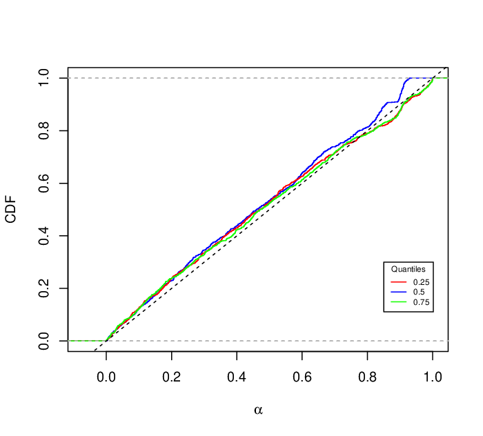
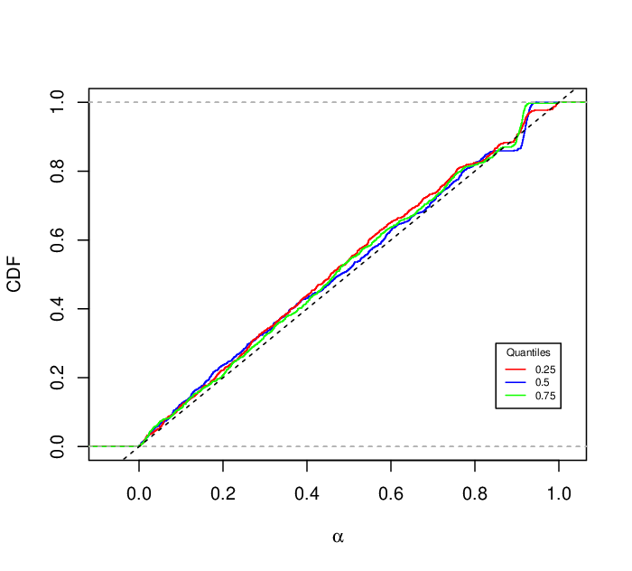
There are a number of different strategies available for constructing confidence intervals for population quantiles. For further illustration, we compare our method to two of them: an exact-but-conservative solution based on the binomial distribution and a basic bootstrap procedure, which resamples the data with replacement, computes the desired quantile and then reports, for a confidence interval, the and quantiles of this bootstrapped distribution. For our simulation, we consider to be a Cauchy distribution with location and scale parameters equal to 2 and 1, respectively. We generated 1000 data sets of size and, from each, 95% confidence intervals for , with , based on the three methods are extracted. Table 1 reports the estimated coverage probabilities and mean length of these intervals. Note that approximately validity of the generalized IM solution is confirmed. Moreover, it is slightly more efficient than both the conservative and basic bootstrap methods.
| GIM | Conservative | Bootstrap | |
|---|---|---|---|
| 0.95 (1.12) | 0.96 (1.23) | 0.96 (1.20) | |
| 0.95 (0.62) | 0.98 (0.69) | 0.96 (0.64) | |
| 0.93 (1.12) | 0.96 (1.25) | 0.94 (1.15) |
4.2 Multivariate median
In univariate analysis, it is well known that the median is a more robust measure of the distribution’s center than the mean. This is also the case in multivariate analysis. However, replacing the multivariate mean by a multivariate median is not so straightforward. Indeed, since multivariate data do not have a natural ordering, there are various different ways of defining an order, each leading to a definition of the multivariate median or, more generally, multivariate quantiles (Becker et al., 2014).
The most common version of a multivariate median is the spatial median. This can be defined similar to the univariate median described above, as the minimizer of a risk function where the loss is given by
where is the usual -norm for vectors in . Alternatively, the spatial median can be defined as a Z-estimator, i.e., it satisfies the system of equations where is a -vector with components
Consistency of the bootstrap for the multivariate median was established recently as part of Theorem 1 in Bhattacharya and Ghosal, 2022.
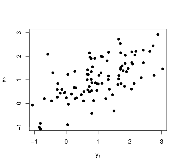
For a quick illustration, Figure 2(a) shows the data for , which are samples from bivariate normal with mean , unit variances, and correlation 0.7. In Figure 2(b), the plausibility contour in (11) is shown, based on the function defined above, with the quadratic form in (8), and . The shaded area in Figure 2(c) represents the 95% plausibility region for derived by (14) and, in black, the classic 95% confidence ellipse based on the asymptotic normality. Note how the IM solution is more efficient. Figure 2(d) shows the resulting empirical distribution of the simulation study where the above scenario is repeated 1000 times and, for each data set, is evaluated. Approximate validity is once again verified. This is also true when a smaller sample of size is considered.


4.3 Quantile regression
Let be a response variable coupled with a covariate . The goal of quantile regression is to estimate the quantile for the conditional distribution of , given . Fix a probability and let denote the conditional quantile of , given . Then the quantile regression model says
where is the vector of regression coefficients of interest. This “model” describes the functional form of the quantile function, but does not determine the distribution of , given . Towards making inference on , Koenker and Bassett, 1978 show that is a risk-minimizer with respect to the loss function
Properties of the quantile regression M-estimator, e.g., its asymptotic normality, are investigated in Koenker, 2005 and, in particular, bootstrap consistency is established in Hahn, 1995. Here we present an illustration of the proposed generalized IM solution to the quantile regression problem.
Let , , with , and let , where , and . Suppose the interest is for . Figure 3(b) displays the data, the estimated quantile regression line corresponding to the Z-estimator . Plausibility contours are obtained for based on the loss function above and , and the plot shows the marginal plausibility contours for at selected values of . The corresponding 95% marginal plausibility band for is shown in Figure 3(a). Approximate validity of the plausibility bands is implied by the approximate validity of the generalized IM. To check this claim empirically, we simulate 1000 data sets according the above scheme and calculated , in each replication. Figure 3(c) shows the empirical distribution of these values over replications and it is clear this closely matches a uniform distribution, confirming Theorem 1. The same plots for and are included and all suggest the uniform approximation for the distribution of is accurate across a range of quantile levels. Figure 3(d) is analogous to Figure 3(c), but considering . As in the previous examples, the proposed solution achieves approximately validity even in finite-sample scenarios.


5 Dynamic treatment regimes
5.1 Introduction
Compared to the common one-size-fits-all approach in medicine, where treatment decisions are developed for the “average” patient, precision medicine focuses on tailoring treatment decisions to individual patients based on certain characteristics of their profile. Dynamic treatment regimes provide a formal precision medicine framework, where the individualization of treatments is dictated by a sequence of decision rules, one per stage of intervention, that are based on the patient’s “history,” which includes both covariates and past treatments (Chakraborty and Murphy, 2014).
In this section, we aim to provide a generalized IM solution to relevant problems that arise when considering dynamic treatment regimes, or regimes for short. For example, given a specific regime, a first basic problem is quantifying uncertainty about the expected outcome if the population under study were to receive treatment according to its rules. This expected outcome is also referred to as the value of a regime. In Section 5.3, we construct a generalized IM for this purpose. A more challenging problem is where there is a large class of candidate decision rules and the goal is to identify an optimal one, i.e., the regime that maximizes the expected benefit to patients based on their history. In Section 5.4 we make the notion of an optimal regime precise, and develop a generalized IM to quantify uncertainty about its value.
Before tackling the above relevant problems, we provide a short background on dynamic treatment regimes and setup the basic notation. The details presented throughout this Section are largely based on Tsiatis et al., 2020.
5.2 Background and notation
For simplicity, our focus throughout this Section will be on the so called single decision problem, where there is only one stage at which a treatment must be selected from among a given set of available options.33 3 We adopt the convention in Tsiatis et al., 2020 that any treatment regime, single or multistage, whose decision rules potentially vary according to baseline and evolving patient information, is dynamic. However, other authors (Murphy et al., 2001, e.g.,) consider single decision regimes as “non-dynamic.” In this situation, a dynamic treatment regime consists of a single rule that takes as input the available patient information and returns as output one of the treatment options. Denote this set of possible treatment action options as . Formally, a dynamic treatment regime is defined as a decision rule , a function that maps an individual’s covariates to a treatment option in , that is, , where is the support of the covariates . Here, we explore only the simplest case where contains two treatment options, e.g., a control/active treatment scenario, so takes as input and returns either 0 or 1.
Let , for , represent the observed data from patients, where and denote, respectively, the treatment received (either 0 or 1), the observed outcome under treatment , and the covariates collected, for the patient. Central to both the definition of the value of a given regime and the notion of the optimal regime, to be explored, respectively, in Sections 5.3 and 5.4 below, is the concept of potential outcome for any regime . Generally speaking, a potential outcome (Rubin, 1974; Rubin, 2005, e.g.,) is the outcome for an individual under a potential treatment. In our context, the random variables and represent the outcome that would be achieved by a randomly chosen individual with covariates in the population of interest if she were to receive treatment 0 or 1, respectively. Note that potential outcomes are hypothetical constructs, since a patient receives only one of the treatments, not both. The idea is to consider what this outcome would have been had the patient received the other treatment option. Now, if treatment is assigned according to regime , the potential outcome of a patient is defined as
| (15) |
We end this subsection by pointing out that the essential results to be explored in the upcoming subsections depend on three fundamental assumptions that are common in the causal inference literature.
- •
Stable unit treatment value assumption: the outcome of a patient who received treatment is the same as her potential outcome for that treatment, i.e.,
- •
No unmeasured confounders assumption: all of the information used to make treatment decisions is captured by the observed covariates , so that
- •
Positivity assumption: For any , there are individuals receiving both treatment options, that is, for .
5.3 Value of a regime
5.3.1 Overview
When considering a specific regime , a fundamental question is how its use in the entire population would affect the outcome of interest, on average. With the definition of a potential outcomes in (15), the value of any regime is defined as
Towards uncertainty quantification of based on observed data , the challenge is deducing the distribution of , which depends on that of , from the distribution of the observable . Under the assumptions stated in the end of Section 5.2, it can be shown that
| (16) |
where the outer expectation is with respect to the marginal distribution of . If we introduce an outcome regression relationship—or Q-function—for the conditional mean,
| (17) |
depending on a parameter ; see (19). Then (16) becomes
| (18) |
5.3.2 Generalized IM construction
First, the simple connection between the Q-function—which depends on a parameter —and the mean of the response allows for a straightforward IM construction for interpreted as a risk minimizer. For a given form describing the Q-function’s dependence on the parameter , we can define a loss function as
Then the generalized IM construction for the minimizer of the expected loss proceeds exactly as in, say, the quantile regression application above. Asymptotic normality of the corresponding M-estimator and consistency of the bootstrap hold for very general Q-function specifications. Note that this generalized IM construction for inference on the risk minimizer does not require that the posited functional form of to be correct. That is, the existence of the risk minimizer does not require that be the true conditional mean of , given and ; moreover, as we discussed in Section 1, if the risk minimizer exists, the it is a “real” inferential target, so drawing inference on the risk minimizer is meaningful whether there is a correctly-specfied model or not.
We are not primarily interested in the aforementioned risk minimizer since, typically, the inferential target is some other characteristic of the problem. Fortunately, these other characteristics can often be expressed as functions of , i.e., as features ; we will consider two such features below. From the previously-described generalized IM for , uncertainty quantification about the value of a given regime is readily obtained through marginalization as discussed in Section 3.2. There is a catch, however, that deserves to be emphasized: these features have their desired interpretation only as functions of the parameter on which the true -function depends. So, in order for marginal inference about these particular features, derived from a generalized IM for , to be meaningful, it is required to assume that the posited form of the Q-function is correctly specified; that is, is not just the risk minimizer but determines the true conditional mean function. Note, however, that this does not require correct specification of a statistical model—which includes distributional forms—for the observable data . The situation we are describing here falls under the general umbrella of semiparametric inference, where only a part of the model is assumed to be correctly specified.
We present the details of our proposed generalized IM in the context of an example. Consider the simulated observational study presented in https://laber-labs.com/dtr-book/booktoc.html,44 4 This is Tsiatis et al., 2020’s companion website, where several examples are provided. The particular example we explore here can be found under the “Chapter 3” tab. whose objective is to assess the effectiveness of a fictitious medication developed for the treatment of hypertension. Each patient in this study either received the new medication () or received no treatment () based on patient/physician discretion. The outcome of interest is the change in systolic blood pressure (mmHg) after six months of treatment, i.e., . The covariates are, respectively, the total cholesterol (mg/dl) and the potassium level (mg/dl). Here is how the data are generated. Let , , with and the constraint . Let , , , where
and , where
This implies an outcome regression relationship in (17) given by
| (19) |
depending on . From the definition of above, the true values of , , , , , and are , , , , and , respectively. Note that the only aspect of the above description that the generalized IM assumes as “true” is the Q-function specification in (19); the statements concerning the distributions of the observables are not used at all in the generalized IM formulation nor are they assumed true in the supporting theory presented in Section 3.4.
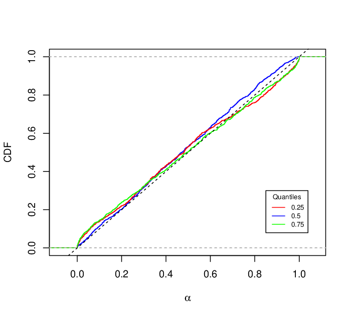
As a first check, we empirically verify the approximate validity claim in Theorem 1 for inference on , the true parameters of the regression function. Figure 4 shows the distribution function of based on repeated sampling from the data-generating process described above, with the true values. As the theory predicts, we see that the distribution of is almost exactly , which means that inference drawn on in this setting is approximately—and almost exactly—valid.

Next, we consider three different marginalization examples. First, in treatment/control scenarios, it is common that the first enquiry performed by the data analyst concerns the presence of a treatment effect. Here the treatment effect is the average change in systolic blood pressure, after six months, if everyone in the population took the new medication compared to if everyone took the old medication. For the Q-function in (19), the treatment effect is , so interest is in the assertion “.” For the particular data , the upper probability assigned to this assertion is approximately 0; this is not particularly surprising, given that the true treatment effect is equal to mmHg.
Second, we investigate marginal inference on the value of a fixed regime. In this case, we consider two such regimes:
- •
the static regime where all individuals are recommended to receive the new medication, i.e., ;
- •
the covariate-dependent regime that assigns patients to receive the treatment if their cholesterol level exceeds a certain threshold, i.e.,
(20)
From (18), the values of the static and covariate dependent regimes are, respectively,
and Figure 5(a) shows the corresponding marginal plausibility contours for each, both obtained from the generalized IM for . The plot suggests that, not unexpectedly, the covariate-dependent regime is no worse than the static regime.
Third, a relevant question in practice might be whether there is a difference between two fixed regimes. For example, given the overlap of the plausibility contours in Figure 5(a), one may wonder if the covariate-dependent regime is in fact better than the static regime. More specifically, interest is whether . Figure 5(b) shows the marginal plausibility contour for the difference , obtained, once again, from the generalized IM for . Despite the differences being small, the assertion “” has zero plausibility, confirming the superiority of the covariate-dependent regime. Whether these small differences are practically relevant is a separate question.


5.4 Optimal regime
Estimating the value of a specific decision rule, , may be of some interest in applications, but a more challenging problem is to identify the optimal regime within a given set , that is, a regime that leads to the best benefit on average if used to select treatment in the population. For situations where larger values of the response variable mean greater benefit to the patient, like in the example in Section 5.3.2 above, the optimal regime is defined as one that leads to the maximum value among all , i.e.,
or, equivalently,
| (21) |
It is possible that more than one regime satisfies (21), but we will not concern ourselves with this technicality here. Recall that our focus is on a single stage treatment regime with . For such a case, Tsiatis et al., 2020 prove that (21) is satisfied by
| (22) |
Just like in the previous subsection, uncertainty quantification about based on observed data requires us to rewrite (5.4) in terms of . Under the assumptions stated at the end of Section 5.2, (5.4) can be equivalently written as
| (23) |
which, under the outcome regression model formulation can itself be rewritten as
| (24) |
Moreover, the value of this optimal treatment is given by
| (25) |
where, again, the outer expectation is with respect to the distribution of . The right-hand side of the above display is, again, a function of , so if we have a generalized IM for , then we can readily obtain a marginal IM for .
As an illustration, consider again the example explored in Section 5.3.2, where is linear as in (19). In this case, it is clear that (24) becomes
From (25), the value of this optimal regime is given by
| (26) |
Uncertainty quantification about the value above is obtained through marginalization, as it was the case for the fixed regimes considered earlier. For example, to obtain the plausibility contour in Figure 5(a), one starts with the generalized IM for and marginalize to the corresponding in (26). Note how the value of is significantly greater than the values of the two fixed regimes also shown in Figure 5.
6 Conclusion
Here we focused on direct, data-driven uncertainty quantification for unknowns defined as risk minimizers or solutions to estimating equations rather than parameters of a statistical model. We presented a new generalized IM that not only avoids the explicit description of the data generating process, but does not require a statistical model at all. We showed that this construction leads to approximately valid uncertainty quantification in the sense of Theorem 1. This provides guarantees beyond those from classical confidence regions. That is, the IM’s validity property applies to belief assignments to all assertions about the inferential target—even marginal inference about features of the original inferential target. To our knowledge, this is the first paper providing direct and valid probabilistic uncertainty quantification in this practically relevant class of learning problems.
Applications in cases beyond the simple, low-dimensional problems above will be reported elsewhere. Of course, larger dimension creates computational challenges, so getting marginal plausibility contours for each component of the high-dimensional inferential target in an efficient way remains an open question. Since evaluation of is based on sampling (bootstrap or Monte Carlo), and marginalization is optimization in this imprecise probability setting, techniques like stochastic approximation or stochastic gradient descent seem especially promising; see, e.g., Syring and Martin, 2021.
We end this section with a brief discussion of some open questions. First, it is well-known that the bootstrap often enjoys a certain higher-order accuracy, that is, the coverage probability of bootstrap-based confidence regions converge to the nominal level at a rate faster than the expected root-; see, e.g., Hall, 1992 and Lehmann, 1999. Similarly, in other settings, with simpler versions of the generalized IM framework developed here, it was observed empirically that the uniform limit distribution approximation for “” was quite accurate, even for small samples, suggesting some higher-order accuracy. The proposed generalized IM in this paper borrows aspects of these two approaches that (at least empirically) enjoy higher-order accuracy. Then the question is if this combination of two higher-order accurate methods is also higher-order accurate?
Second, although this did not appear in our illustrations in Section 5, an especially challenging aspect of the dynamic treatment regime problem is non-regularity, resulting from the non-smooth “max” operator in (23), that affects the limit distribution theory of the M/Z-estimators and, in turn, the corresponding bootstrap-based inference. A common remedy for failure of the bootstrap, e.g., due to non-regularity, is to “under-sample” with the so-called m-out-of-n bootstrap. That is, Bickel et al., 1997 showed that, by taking bootstrap samples of size , bootstrap failure could be avoided. A more sophisticated -out-of- bootstrap scheme was proposed in Chakraborty et al., 2013 that could prevent bootstrap failure in the dynamic treatment regime setting resulting from the non-regularity induced by the “max” operator. An interesting follow-up project could investigate the reliability of the proposed generalized IM equipped with a -out-of- bootstrap strategy under non-regularity.
Acknowledgments
The authors thank the Guest Editor and the two anonymous reviewers for their helpful feedback on a previous version of this manuscript. This work is partially supported by the U.S. National Science Foundation, grants DMS–1811802 and SES–2051225.
References
- Balch et al., (2019) Balch, M. S., Martin, R., and Ferson, S. (2019). Satellite conjunction analysis and the false confidence theorem. Proceedings of the Royal Society A: Mathematical, Physical and Engineering Sciences, 475(2227):20180565.
- Becker et al., (2014) Becker, C., Fried, R., and Kuhnt, S. (2014). Robustness and Complex Data Structures: Festschrift in Honour of Ursula Gather. SpringerLink : Bücher. Springer Berlin Heidelberg.
- Bhattacharya and Ghosal, (2022) Bhattacharya, I. and Ghosal, S. (2022). Bayesian inference on multivariate medians and quantiles. Statistica Sinica, 32(1):517–538.
- Bickel and Freedman, (1981) Bickel, P. J. and Freedman, D. A. (1981). Some asymptotic theory for the bootstrap. The Annals of Statistics, 9(6):1196–1217.
- Bickel et al., (1997) Bickel, P. J., Götze, F., and van Zwet, W. R. (1997). Resampling fewer than observations: gains, losses, and remedies for losses. Statistica Sinica, 7(1):1–31.
- Boos and Stefanski, (2013) Boos, D. D. and Stefanski, L. A. (2013). Essential Statistical Inference. Springer Texts in Statistics. Springer, New York.
- Cahoon and Martin, (2020) Cahoon, J. and Martin, R. (2020). Generalized inferential models for meta-analyses based on few studies. Statistics and Applications, 18(2):299–316.
- Cahoon and Martin, (2021) Cahoon, J. and Martin, R. (2021). Generalized inferential models for censored data. International Journal of Approximate Reasoning, 137:51–66.
- (9) Cella, L. and Martin, R. (2021a). Approximately valid and model-free possibilistic inference. In Denœux, T., Lefèvre, E., Liu, Z., and Pichon, F., editors, Belief Functions: Theory and Applications, pages 127–136, Cham. Springer International Publishing.
- (10) Cella, L. and Martin, R. (2021b). Valid inferential models for prediction in supervised learning problems. In Cano, A., De Bock, J., Miranda, E., and Moral, S., editors, Proceedings of the Twelveth International Symposium on Imprecise Probability: Theories and Applications, volume 147 of Proceedings of Machine Learning Research, pages 72–82. PMLR. Extended version available at https://researchers.one/articles/21.12.00002v1.
- Cella and Martin, (2022) Cella, L. and Martin, R. (2022). Validity, consonant plausibility measures, and conformal prediction. International Journal of Approximate Reasoning, 141:110–130.
- Chakraborty et al., (2013) Chakraborty, B., Laber, E. B., and Zhao, Y. (2013). Inference for optimal dynamic treatment regimes using an adaptive -out-of- bootstrap scheme. Biometrics, 69(3):714–723.
- Chakraborty and Murphy, (2014) Chakraborty, B. and Murphy, S. A. (2014). Dynamic treatment regimes. Annual Review of Statistics and Its Application, 1(1):447–464.
- Chatterjee and Bose, (2005) Chatterjee, S. and Bose, A. (2005). Generalized bootstrap for estimating equations. The Annals of Statistics, 33(1):414 – 436.
- Cheng and Huang, (2010) Cheng, G. and Huang, J. (2010). Bootstrap consistency for general semiparametric M-estimation. The Annals of Statistics, 38(5):2884–2915.
- Choquet, (1954) Choquet, G. (1953–1954). Theory of capacities. Université de Grenoble. Annales de l’Institut Fourier, 5:131–295 (1955).
- Conover, (1971) Conover, W. (1971). Practical Nonparametric Statistics. Wiley.
- Cui and Hannig, (2019) Cui, Y. and Hannig, J. (2019). Nonparametric generalized fiducial inference for survival functions under censoring. Biometrika, 106(3):501–518.
- Cunen et al., (2020) Cunen, C., Hjort, N. L., and Schweder, T. (2020). Confidence in confidence distributions! Proceedings of the Royal Society A: Mathematical, Physical and Engineering Sciences, 476(2237):20190781.
- Dawid and Stone, (1982) Dawid, A. P. and Stone, M. (1982). The functional-model basis of fiducial inference. The Annals of Statistics, 10(4):1054 – 1067.
- Dempster, (1968) Dempster, A. P. (1968). A generalization of Bayesian inference. (With discussion). Journal of the Royal Statistical Society, Series B, 30:205–247.
- Dempster, (2008) Dempster, A. P. (2008). The Dempster–Shafer calculus for statisticians. International Journal of Approximate Reasoning, 48(2):365 – 377.
- Dempster, (2014) Dempster, A. P. (2014). Statistical inference from a Dempster–Shafer perspective. In Lin, X., Genest, C., Banks, D. L., Molenberghs, G., Scott, D. W., and Wang, J.-L., editors, Past, Present, and Future of Statistical Science, chapter 24. Chapman & Hall/CRC Press.
- Denœux, (2009) Denœux, T. (2009). Extending stochastic ordering to belief functions on the real line. Information Sciences, 179(9):1362–1376.
- Denœux, (2014) Denœux, T. (2014). Likelihood-based belief function: justification and some extensions to low-quality data. International Journal of Approximate Reasoning, 55(7):1535–1547.
- Dubois and Prade, (1986) Dubois, D. and Prade, H. (1986). The principle of minimum specificity as a basis for evidential reasoning. In Proceedings of International Conference on Information Processing and Management of Uncertainty in Knowledge-based Systems, pages 75–84. Springer.
- Dubois and Prade, (1988) Dubois, D. and Prade, H. (1988). Possibility Theory. Plenum Press, New York.
- Efron, (1979) Efron, B. (1979). Bootstrap methods: Another look at the jackknife. The Annals of Statistics, 7(1):1–26.
- Fisher, (1935) Fisher, R. A. (1935). The fiducial argument in statistical inference. Annals of Eugenics, 6(4):391–398.
- Fisher, (1973) Fisher, R. A. (1973). Statistical Methods and Scientific Inference. Hafner Press, New York, 3rd edition.
- Fraser, (1968) Fraser, D. A. S. (1968). The Structure of Inference. John Wiley & Sons Inc., New York.
- Fraser, (2011) Fraser, D. A. S. (2011). Is Bayes posterior just quick and dirty confidence. Statistical Science, 26:299–316.
- Ghosal and van der Vaart, (2017) Ghosal, S. and van der Vaart, A. (2017). Fundamentals of Nonparametric Bayesian Inference, volume 44 of Cambridge Series in Statistical and Probabilistic Mathematics. Cambridge University Press, Cambridge.
- Ghosh and Ramamoorthi, (2003) Ghosh, J. and Ramamoorthi, R. (2003). Bayesian Nonparametrics. Springer Series in Statistics. Springer.
- Godambe, (1991) Godambe, V. (1991). Estimating Functions. Oxford Science Publications. Clarendon Press.
- Hahn, (1995) Hahn, J. (1995). Bootstrapping quantile regression estimators. Econometric Theory, 11(1):105–121.
- Hall, (1992) Hall, P. (1992). The Bootstrap and Edgeworth Expansion. Springer Series in Statistics. Springer-Verlag, New York.
- Hannig et al., (2016) Hannig, J., Iyer, H., Lai, R. C. S., and Lee, T. C. M. (2016). Generalized fiducial inference: A review and new results. Journal of the American Statistical Association, 111(515):1346–1361.
- Hjort et al., (2010) Hjort, N. L., Holmes, C. C., Müller, P., and Walker, S. G., editors (2010). Bayesian Nonparametrics. Cambridge University Press.
- Hose and Hanss, (2021) Hose, D. and Hanss, M. (2021). A universal approach to imprecise probabilities in possibility theory. International Journal of Approximate Reasoning, 133:133–158.
- Huber, (1981) Huber, P. (1981). Robust Statistics. Wiley Series in Probability and Statistics. Wiley.
- Huber, (1964) Huber, P. J. (1964). Robust estimation of a location parameter. The Annals of Mathematical Statistics, 35(1):73 – 101.
- Koenker, (2005) Koenker, R. (2005). Quantile Regression. Cambridge University Press, Cambridge.
- Koenker and Bassett, (1978) Koenker, R. and Bassett, G. (1978). Regression quantiles. Econometrica, 46(1):33–50.
- Kosorok, (2008) Kosorok, M. (2008). Introduction to Empirical Processes and Semiparametric Inference. Springer Series in Statistics. Springer New York.
- Lehmann, (1999) Lehmann, E. L. (1999). Elements of Large-Sample Theory. Springer Texts in Statistics. Springer-Verlag, New York.
- Liu and Martin, (2021) Liu, C. and Martin, R. (2021). Inferential models and possibility measures. Handbook of Bayesian, Fiducial, and Frequentist Inference, to appear; arXiv:2008.06874.
- Martin, (2015) Martin, R. (2015). Plausibility functions and exact frequentist inference. Journal of the American Statistical Association, 110(512):1552–1561.
- Martin, (2018) Martin, R. (2018). On an inferential model construction using generalized associations. Journal of Statistical Planning and Inference, 195:105–115.
- Martin, (2019) Martin, R. (2019). False confidence, non-additive beliefs, and valid statistical inference. International Journal of Approximate Reasoning, 113:39–73.
- Martin, (2021) Martin, R. (2021). An imprecise-probabilistic characterization of frequentist statistical inference. Researchers.One, https://researchers.one/articles/21.01.00002.
- Martin, (2022) Martin, R. (2022). Valid and efficient imprecise-probabilistic inference across a spectrum of partial prior information. https://researchers.one/articles/21.05.00001.
- Martin et al., (2021) Martin, R., Balch, M. S., and Ferson, S. (2021). Response to the comment confidence in confidence distributions! Proceedings of the Royal Society A: Mathematical, Physical and Engineering Sciences, 477(2250):20200579.
- Martin and Liu, (2013) Martin, R. and Liu, C. (2013). Inferential models: A framework for prior-free posterior probabilistic inference. Journal of the American Statistical Association, 108:301–313.
- Martin and Liu, (2015) Martin, R. and Liu, C. (2015). Inferential Models: Reasoning with Uncertainty. Monographs in Statistics and Applied Probability Series. Chapman & Hall/CRC Press.
- Martin and Syring, (2022) Martin, R. and Syring, N. (2022). Direct Gibbs posterior inference on risk minimizers: construction, concentration, and calibration. In Handbook of Statistics: Advancements in Bayesian Methods and Implementation, to appear; arXiv:2203.09381.
- Molchanov, (2005) Molchanov, I. (2005). Theory of Random Sets. Probability and Its Applications (New York). Springer-Verlag London Ltd., London.
- Murphy et al., (2001) Murphy, S. A., van der Laan, M. J., Robins, J. M., and Group, C. P. P. R. (2001). Marginal mean models for dynamic regimes. Journal of the American Statistical Association, 96(456):1410–1423. PMID: 20019887.
- Nguyen, (2006) Nguyen, H. T. (2006). An Introduction to Random Sets. Chapman & Hall/CRC, Boca Raton, FL.
- Reid and Cox, (2015) Reid, N. and Cox, D. R. (2015). On some principles of statistical inference. International Statistical Review, 83(2):293–308.
- Rubin, (1974) Rubin, D. B. (1974). Estimating causal effects of treatments in randomized and nonrandomized studies. Journal of Educational Psychology., 66(5):688–701.
- Rubin, (2005) Rubin, D. B. (2005). Causal inference using potential outcomes. Journal of the American Statistical Association, 100(469):322–331.
- Schweder and Hjort, (2016) Schweder, T. and Hjort, N. L. (2016). Confidence, Likelihood, Probability: Statistical Inference with Confidence Distributions. Cambridge Series in Statistical and Probabilistic Mathematics. Cambridge University Press.
- Shafer, (1976) Shafer, G. (1976). A Mathematical Theory of Evidence. Princeton University Press, Princeton, N.J.
- Shao and Tu, (1995) Shao, J. and Tu, D. S. (1995). The Jackknife and Bootstrap. Springer Series in Statistics. Springer-Verlag, New York.
- Singh, (1981) Singh, K. (1981). On the asymptotic accuracy of Efron’s bootstrap. The Annals of Statistics, 9(6):1187–1195.
- Syring and Martin, (2021) Syring, N. and Martin, R. (2021). Stochastic optimization for numerical evaluation of imprecise probabilities. In Cano, A., De Bock, J., Miranda, E., and Moral, S., editors, Proceedings of the Twelveth International Symposium on Imprecise Probability: Theories and Applications, volume 147 of Proceedings of Machine Learning Research, pages 289–298. PMLR.
- Tsiatis et al., (2020) Tsiatis, A. A., Davidian, M., Holloway, S. T., and Laber, E. B. (2020). Dynamic Treatment Regimes: Statistical Methods for Precision Medicine. Chapman & Hall/CRC.
- van der Vaart and Wellner, (1996) van der Vaart, A. W. and Wellner, J. A. (1996). Weak Convergence and Empirical Processes. Springer-Verlag, New York.
- Walley, (2002) Walley, P. (2002). Reconciling frequentist properties with the likelihood principle. Journal of Statistical Planning and Inference, 105:35–65.
- Wasserman, (2006) Wasserman, L. (2006). All of Nonparametric Statistics. Springer Texts in Statistics. Springer New York.
- Wellner and Zhang, (1996) Wellner, J. A. and Zhang, Y. (1996). Bootstrapping Z-estimators. Technical Report 308, University of Washington. https://stat.uw.edu/research/tech-reports/bootstrapping-z-estimators.
- Xie and Singh, (2013) Xie, M.-g. and Singh, K. (2013). Confidence distribution, the frequentist distribution estimator of a parameter: A review. International Statistical Review, 81(1):3–39.
- Zadeh, (1975) Zadeh, L. A. (1975). Fuzzy logic and approximate reasoning. Synthese, 30(3-4):407–428.