Revisiting Memory Efficient Kernel Approximation:
An Indefinite Learning Perspective -
Supplementary Material
Simon Heilig Maximilian Münch Frank-Michael Schleif
University of Bamberg UAS Würzburg-Schweinfurt, University of Groningen UAS Würzburg-Schweinfurt
1 INTRODUCTION
As derived in the paper, MEKA can be used with a large variety of practical relevant kernel functions as long as some moderate constraints, such as the normalization of the input space and a data compactness hypothesis by means of an inherent block-cluster structure, are fulfilled. Subsequently, we provide additional results and details:
- -
Section 2 provides a brief orientation of the implementation given in the supplement folder.
- -
Section 3 shows additional non-stationary kernel matrices with block-wise structure.
- -
Section 4 provides additional results of negative eigenvalue analysis.
- -
Section 5 presents an out-of-sample extension to the corrected MEKA approximation.
- -
Section 6 presents further experimental information, like hyperparameters and approximation error.
- -
Section 7 presents an overview of utilized kernel functions and their relevant properties.
2 REFACTORED AND EXTENDED IMPLEMENTATION
The code of this paper is written in Matlab and can be found at: https://github.com/simonheilig/indefinite-meka. It is structured as follows:
The folder MEKA contains all code of the MEKA approximation, which is a refactored version of Si et al., 2017 extended for a generic use of kernel functions with the Lanczos iteration based shift correction (main file: meka.m). Folder kernels contains all implemented kernel functions and the folder experiments consists of two parts, first the analysis of negative eigenvalues and second, the classification experiments (main files: setupEigenvalues.m, setupClassification.m). The data sets are together with the generation script provided in folder data.
3 BLOCK-WISE STRUCTURE IN NON-STATIONARY KERNELS
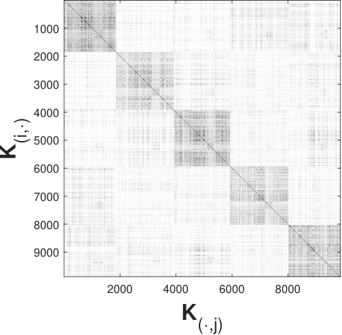
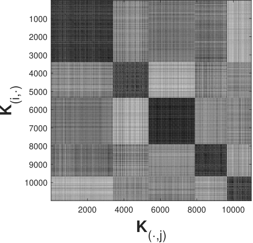
In our work, we extended the use of MEKA to non-stationary kernels by applying a projection to the unit sphere in the input space (See Proposition 1 and Section 3.2). Figure 1 shows an excerpt of the kernel matrices obtained with non-stationary kernel functions.
It is clearly visible, that a block-wise structure is created after clustering in the input space and thereafter rearranging the respective kernel matrix. Together with the results of the experiments conducted in the main paper, this emphasizes the approximation capabilities of MEKA in case of non-stationary kernel functions.
 |
 |
 |
 |
| (a) | (b) | (c) | (d) |
4 OCCURRENCE OF NEGATIVE EIGENVALUES
In the paper we studied the occurrence of invalid kernel approximations and in the following the remaining results are presented. Figures 2-6 illustrate the remaining Gaussian rbf kernel results and Figures 7-11 focus on the extreme learning kernel. (a) shows in the following figures the relative approximation error along the different target ranks and numbers of clusters, (b) presents the value of the smallest eigenvalue and (c) shows the total number of negative eigenvalues.
It is apparent that the evaluations show similar results, by means that MEKA achieves lower approximation error with higher rank and produces among all constellations a non-negligible amount of negative eigenvalues. It is also noteworthy that a higher target rank leads to a higher amount of negative eigenvalues, as it can be consistently seen in Figures 2-6 (c).
| (a) | (b) | (c) |
| (a) | (b) | (c) |
| (a) | (b) | (c) |
| (a) | (b) | (c) |
| (a) | (b) | (c) |
| (a) | (b) | (c) |
| (a) | (b) | (c) |
| (a) | (b) | (c) |
| (a) | (b) | (c) |
| (a) | (b) | (c) |
5 OUT-OF-SAMPLE EXTENSION
If the model has to be applied to new data points, one would like to modify them in a consistent way with respect to the training scenario. In our proposal we provide a strategy for a shift correction and a normalization, which plays a key role and needs to be taken into account, if a new test point is considered.
The training model finally consists of the matrices , the link matrix a shift parameter and an index set (block-wise denoted as ), referring to known reference points. Further, the self-similarities of the training points need to be stored if a normalization is required for a non-stationary kernel function.
The challenge of an out-of-sample extension can be solved in different ways, here we suggest two strategies:
(1) In the direct approach, one needs to calculate the kernel evaluations of , with respect to some , e.g. the support vectors, needed in the prediction model. This is done directly on the original, unapproximated kernel function. If the kernel function has to be normalized an additional step, as shown in Remark 1, is required. Note that by evaluating self similarities the parameter needs to be added. This approach is particular useful if the MEKA approximation is very accurate and the evaluation of the kernel function is cheap.
(2) The indirect approach maps the new point in the approximated kernel representation as follows. From the MEKA algorithm part 2 we have stored the landmark matrices of each cluster . Additionally, we need to store the cluster-wise matrices (from the SVD) used to generate , which is rather cheap. Now we calculate the similarities of for each block , using the original kernel function, where are the landmark indices of block . These small landmark vectors are used to generate an extended . From the enlarged a block-matrix is constructed and can be used in the same way as in the MEKA approach. Additional modifications regarding the shift correction and normalization can be applied as shown before.
6 CLASSIFICATION EXPERIMENT INFORMATION
Typical hyperparameters which are obtained in the classification experiments from Section 4.3 are listed in Table 1. Note that the overall rank approximation is times , since the same rank per cluster strategy was used. The parameters are tuned with a grid-search and 5-fold cross-validation. The classification results were collected via a 10-fold cross-validation and the hyperparameter tuning was executed in each fold. Hence, Table 1 provides just an excerpt of the utilized parameters.
| Dataset | ID | |||||||||
|---|---|---|---|---|---|---|---|---|---|---|
| spambase | 1 | 128 | 3 | 0.1 | 39.9 | 10;2 | 1000 | 1000 | 1000 | 1 |
| artificial 1 | 2 | 64 | 3 | 1 | 1.4 | 8;2 | 100 | 1 | 1000 | 10 |
| cpusmall | 3 | 16 | 3 | 10 | 8.4 | 10;2 | 10 | 10 | 1000 | 1 |
| gesture | 4 | 16 | 3 | 15 | 22.4 | 10;2 | 1000 | 1000 | 100 | 1 |
| artificial 2 | 5 | 16 | 3 | 0.1 | 10.5 | 2;3 | 100 | 1 | 1 | 1 |
| pendigit | 6 | 16 | 3 | 1 | 11.2 | 8;3 | 10 | 100 | 100 | 100 |
In Table 2 the relative approximation error of the matrices used in the classification experiments from Section 4.3 are presented. Note that the approximation error of the corrected matrix depends heavily on the magnitude of the shift parameter, as shown in the error bound of Section 4.2. Although the reconstruction error of the corrected matrix worsens in some cases, at the same time, the classification accuracy does not suffer from this effect.
| RBF | Elm | Poly | TL1 | ||||||
|---|---|---|---|---|---|---|---|---|---|
| Dataset | ID | M1 | M2 | M1 | M2 | M1 | M2 | M1 | M2 |
| spambase | 1 | 0.01 | 0.35 | 0.17 | 5.30 | 0.01 | 0.49 | 0.00 | 0.10 |
| (0.01) | (0.57) | (0.03) | (2.23) | (0.01) | (0.51) | (0.00) | (0.06) | ||
| artificial 1 | 2 | 0.00 | 0.00 | 0.00 | 0.02 | 0.00 | 0.00 | 0.01 | 0.18 |
| (0.00) | (0.00) | (0.00) | (0.02) | (0.00) | (0.00) | (0.00) | (0.13) | ||
| cpusmall | 3 | 0.11 | 2.92 | 0.06 | 1.66 | 0.00 | 0.00 | 0.00 | 0.04 |
| (0.04) | (1.93) | (0.02) | (0.70) | (0.00) | (0.00) | (0.00) | (0.03) | ||
| gesture | 4 | 0.22 | 23.41 | 0.06 | 1.61 | 0.47 | 18.09 | 0.01 | 0.20 |
| (0.07) | (10.86) | (0.02) | (0.40) | (0.04) | (8.98) | (0.00) | (0.03) | ||
| artificial 2 | 5 | 0.00 | 0.02 | 0.07 | 2.70 | 0.00 | 0.00 | 0.00 | 0.02 |
| (0.00) | (0.01) | (0.01) | (0.58) | (0.00) | (0.00) | (0.00) | (0.01) | ||
| pendigit | 6 | 0.21 | 5.82 | 0.09 | 2.71 | 0.00 | 0.03 | 0.00 | 0.06 |
| (0.05) | (3.98) | (0.01) | (0.30) | (0.00) | (0.02) | (0.00) | (0.01) | ||
7 KERNEL PROPERTIES
Table 3 presents a brief overview of the different kernel functions used in this paper. We do not claim completeness of the listed properties and literature references but show information to support the relevance of an extended MEKA approach. The kernel properties of the Gaussian rbf and polynomial kernel are collected from Shawe-Taylor and Cristianini, 2004 and in case of the other kernels the information are obtained from the first publishing paper.
| Kernel | Properties | Publications | Preprocessing |
|---|---|---|---|
| Gaussian rbf | , , , infinite dimensional feature space, unitary-invariant, shift-invariant | introduced in Schölkopf et al., 1997 for the SVM; among other things it is used for kernel based methods on EEG signals (Bajoulvand et al., 2017), opinion mining and sentiment analysis (Gopi et al., 2020), ground penetrating radar analysis (Tbarki et al., 2016) | -Normalization |
| Polynomial | , dimensional feature space, unitary-invariant, non-stationary | first used by Poggio, 1975; among other things it is used for termite detection (Achirul Nanda et al., 2018), person re-identification (Chen et al., 2015), speaker verification (Yaman and Pelecanos, 2013) | L2-Normalization |
| Extreme Learning | parameter-insensitive, rbf alternative, differentiable, non-stationary | introduced in Frénay and Verleysen, 2011; among other things it is used for clustering by fuzzy neural gas (Geweniger et al., 2013), alumina concentration estimation (Zhang et al., 2017), predicting wear loss (Ulas et al., 2020) | ()-Normalization, L2-Normalization |
| Truncated Manhattan | , two-level deep piecewise linear, compactly supported, indefinite, stable performance, shift-invariant | introduced in Huang et al., 2017b; among other things it is used in LS-SVM and PCA (Huang et al., 2017a), piecewise linear kernel support vector clustering (Shang et al., 2017) | -Normalization |
References
- Achirul Nanda et al., (2018) Achirul Nanda, M., Boro Seminar, K., Nandika, D., and Maddu, A. (2018). A comparison study of kernel functions in the support vector machine and its application for termite detection. Information, 9(1):5.
- Bajoulvand et al., (2017) Bajoulvand, A., Zargari Marandi, R., Daliri, M. R., and Sabzpoushan, S. H. (2017). Analysis of folk music preference of people from different ethnic groups using kernel-based methods on eeg signals. Applied Mathematics and Computation, 307:62–70.
- Chen et al., (2015) Chen, D., Yuan, Z., Hua, G., Zheng, N., and Wang, J. (2015). Similarity learning on an explicit polynomial kernel feature map for person re-identification. In Proceedings of the IEEE Conference on Computer Vision and Pattern Recognition, pages 1565–1573.
- Frénay and Verleysen, (2011) Frénay, B. and Verleysen, M. (2011). Parameter-insensitive kernel in extreme learning for non-linear support vector regression. Neurocomputing, 74(16):2526–2531.
- Geweniger et al., (2013) Geweniger, T., Fischer, L., Kaden, M., Lange, M., and Villmann, T. (2013). Clustering by fuzzy neural gas and evaluation of fuzzy clusters. Computational intelligence and neuroscience, 2013.
- Gopi et al., (2020) Gopi, A. P., Jyothi, R. N. S., Narayana, V. L., and Sandeep, K. S. (2020). Classification of tweets data based on polarity using improved rbf kernel of svm. International Journal of Information Technology, pages 1–16.
- (7) Huang, X., Maier, A., Hornegger, J., and Suykens, J. A. (2017a). Indefinite kernels in least squares support vector machines and principal component analysis. Applied and Computational Harmonic Analysis, 43(1):162–172.
- (8) Huang, X., Suykens, J. A. K., Wang, S., Hornegger, J., and Maier, A. (2017b). Classification With Truncated Distance Kernel. IEEE Transactions on Neural Networks and Learning Systems, 29(5):2025–2030.
- Poggio, (1975) Poggio, T. (1975). On optimal nonlinear associative recall. Biological Cybernetics, 19(4):201–209.
- Schölkopf et al., (1997) Schölkopf, B., Sung, K.-K., Burges, C. J., Girosi, F., Niyogi, P., Poggio, T., and Vapnik, V. (1997). Comparing support vector machines with gaussian kernels to radial basis function classifiers. IEEE Transactions on Signal Processing, 45(11):2758–2765.
- Shang et al., (2017) Shang, C., Huang, X., and You, F. (2017). Data-driven robust optimization based on kernel learning. Computers & Chemical Engineering, 106:464–479.
- Shawe-Taylor and Cristianini, (2004) Shawe-Taylor, J. and Cristianini, N. (2004). Kernel methods for pattern analysis. Cambridge university press.
- Si et al., (2017) Si, S., Hsieh, C.-J., and Dhillon, I. (2017). Memory efficient kernel approximation. The Journal of Machine Learning Research, 18(1):682–713.
- Tbarki et al., (2016) Tbarki, K., Said, S. B., Ksantini, R., and Lachiri, Z. (2016). Rbf kernel based svm classification for landmine detection and discrimination. In 2016 International Image Processing, Applications and Systems (IPAS), pages 1–6. IEEE.
- Ulas et al., (2020) Ulas, M., Altay, O., Gurgenc, T., and Özel, C. (2020). A new approach for prediction of the wear loss of pta surface coatings using artificial neural network and basic, kernel-based, and weighted extreme learning machine. Friction, 8(6):1.
- Yaman and Pelecanos, (2013) Yaman, S. and Pelecanos, J. (2013). Using polynomial kernel support vector machines for speaker verification. IEEE Signal Processing Letters, 20(9):901–904.
- Zhang et al., (2017) Zhang, S., Zhang, T., Yin, Y., and Xiao, W. (2017). Alumina concentration detection based on the kernel extreme learning machine. Sensors, 17(9):2002.