A model for calculating volumes of trains as flows given demand and capacity restriction
Abstract
This report presents a novel approach to calculate volumes of trains from a set of requirements describing the transportation demands. The model presented is based on a multi commodity network flow model. The model comprises three different layers: the demand level in which the requirements on the transports are presented, the route layer which describes the routes possible to implement the demands and the flow layer in which the resulting flows of train volumes are calculated and distributed over discrete time periods. This structure corresponds well to other industrial planning processes where different products or services that are to be accomplished are first decomposed by methods into different layers of tasks, by e.g. a work breakdown structure (WBS). Resources are then allocated to the tasks as well as scheduled in time. The most important feature of the proposed model is that it is volume based, i.e. volume of trains are handled instead of scheduling individual trains. Scheduling a timetable is a very complex task, and by concentrating on the volumes of trains over time rather than the detailed scheduling of them, the complexity is greatly reduced which is a large computational advantage. The disadvantage is that the representation of capacity in terms of volumes of trains with different properties becomes crucial. The report discusses these advantages and disadvantages as well as gives two examples of the use of the model.
The work presented in this report has been supported by the Swedish Transport Administration (Trafikverket) under grant TRV2019/132113.
1 Introduction
The following report describes how a operations research model, a multi commodity network flow model (MCNF), can be used for computing train volumes from train demands, over a railway network consisting of stations and links using routing information. The model is intended to be used in a framework where it is used together with another model for scheduling TCRs, Temporary Capacity Restrictions. The framework and the model for scheduling TCRs based on traffic availability is presented in another parallel report [3]. Given named routes together with volumes entering and exiting the railway network the MCNF model calculates the train volumes together with the capacity usage on the link. Crucial for the model to work is the how link capacity is represented in terms of number of trains per time frame, dependent on the heterogeneous mix of train types, since no actual scheduling of individual trains is performed. The solution is a flow of train volumes over the railway network over discrete time periods.
The proposed model have three connected layers. On top of the basic MCNF model are two other layers to handle the fact that different traffic demands can be implemented by different realizations in terms of different routes. The topmost layer is the demand layer, where demands on volumes of traffic are expressed. The basis for this are origin-destination pairs (possibly with via-locations) together with the train type and other basic properties together with the volume of trains departing in each time period. This layer corresponds to the demands from railway undertakers (RUs). The middle layer corresponds to the way the transport is being produced, and corresponds to the term “method” in some other industry sectors. A demand of a large volume of trains can be implemented by several different routes, thereby having different ways of producing the demand.
This three layer approach is found in many industry sectors as well as in most problem solving methodologies. On a high level a task is first split into subtask by methods (describing capabilities) or break down structures. The subtasks can in turn be further detailed until a level where all activities are atomic and in some sense “basically understood”. Resources are allocated to these activities which are then scheduled to get a plan such that no resources are overbooked. This results in a valid plan that accomplish the high end goal. Often the different activities from the first break down structure are contractually bound when the should be ready.
The levels are often used in different process steps, typically the strategic plan is rolling every year with a 36 month coverage, a 24 mount tactical plan and a 12-0 operations process.
The report has three main parts. We first introduce the layered approach and how it fits into the framework of planning temporary capacity restrictions as well as a tool for determining a supply or offer of train volumes. Then the complete mathematical model is presented with some detailed explanations. Lastly two experimental setups are given, one smaller to demonstrate some of the features of the model and one larger to give one of the intended uses of the model.
2 Multi commodity flow network flow model
A multi commodity network flow model (MCNF) [1] is an operations research model. A network flow model is a directed graph where each arc has a capacity which must be greater than or equal to the flow passing that arc. It is also possible to have capacity on the nodes although we have not elaborated on that in this report. Network flows are an important special case of linear programming models, since they (often) preserve the integer property, i.e. if all source and sink flows are integer, then so are the flows on the arcs. A MCNF model, however, does not preserve the integer property, unless the flows of commodities are non-overlapping in the capacity restrictions in which case each commodity flow problem can be modeled separately as a network flow problem. In the model presented in this paper this is not a problem since the volumes of trains are spread out over several time periods, thus it is not individual trains but volumes of trains that flows over the arcs.
There are one or more sources (nodes) where flow enters the graph, and one or more sinks (nodes) where flow is leaving the graph. Each node must fulfill a balance restriction, the sum of incoming flow to each node must equal the outgoing flow. Special cases are the sources and sinks and are modeled differently in the literature. We will regard incoming and outgoing flows as arc coming from a special kind of nodes whose only purpose is to act as source or sink.
MCNF is a network flow model where the flows are of different types, so called commodities. In each node the sum of incoming commodity must equal the sum of outgoing commodity, so the network keeps track of the commodities along the arcs and nodes. The source and sinks are also extended to be of different commodity types.
The basic formulation of a MCNF problem can be stated as:
where is the flow of commodity on arc , is the capacity on arc and is either a source node for (positive value) or a sink node for (negative value) or a transit node (zero).
The commodities in the MCNF model presented in this paper are train services characterized by their origin, destination and type, e.g. commuter train, long distance passenger train, freight trains. The are based on what is called Train Service Classes, TSC [2], see section 3. The network is a graph based on the original railway network (i.e. stations and lines) and extended to implement flow of train volumes over time periods.
Let be a set of time periods then each node and link of the railway network is transformed into a graph with:
- •
nodes for each station node, one node for each time period. Call these timed nodes.
- •
Each resulting timed node is connected with an inventory arc to its consecutive timed node. These hold the volumes that stands on the station from one time period to the next.
- •
Each line between two stations in the railway network is replaced with arcs between the same stations, the first arcs, called direct arcs, are between the stations in each time period, the next arcs connects consecutive time periods and are called next arcs.
in figure 1 this is shown. All arcs are connected to other nodes, forming a network.

A small generic example of the network is presented in figure 2 for a railway network consisting of three stations A, B and C and tracks (directed traffic) A to B and B to C.

Each line in the geographical network has a total capacity, measured as a number of units per time period. Certain volumes of train traffic types consumes more units than other train types, therefore the mix of different train type volumes are important. The sum of all commodities on a line in a time period must not exceed the capacity of that line.
Consumed capacity on a line for a time period is calculated as the sum of all commodities on the direct arcs of that line, half of the next arcs going into the current time period and half of the next arcs going out from the current time period. This is illustrated with the green box in figure 3.

This means that the model does not schedule individual trains but calculates volumes of trains (of different commodities), characterized by their type, origin and destination, as described in their Train Service Classes, TSC, in each time period. Different train types can consume different amount of capacity and the total capacity consumed must obey the capacity restriction on each link.
Since it is volumes of trains in each time period, in principle no further details about when inside the time period the trains will depart is known. All that is known is the number of each TSC (commodity) that will use the line that particular time period. Also note that the number of units consumed by each TSC is a real number, indicating the “spread” of the actual departure/arrival over time. The volumes of each TSC that are flowing into the system in each time period are given (i.e. they are added through the timed source node), as are the the amount of output flows of the TSC in each timed sink node. By these “departure earliest at” and “arrives latest at” it is possible to restrict the volumes of the TSC through the network so that the volumes actually are flowing according to the train type’s traversal times along the links together with a certain “spread” to facilitate meeting and overtakes (The order of the trains are not scheduled by the flow model, see section 4.4 which discusses ways of representing capacity as a function of traffic heterogeneity). Also note that volumes may be split on both the direct and next arcs making the values on the arcs to be real rather than integers, making the consumed capacity real.
3 Traffic Service Classes and Transport Paths
Traffic Service Classes (TSC) are classes of traffic with equal properties. The basic properties are the origin, destination, possibly via-stations, principal performance, possibly axle loads and other restricting properties, and possibly also time period restrictions (e.g. not available during certain times of the day). These TSCs are the commodities, “products” or “package services” available to order or apply for.
A mapping is associated with the TSCs. This mapping describes the principal “method” to implement the packaged service. Each “method” consists of a detailed route through the railway net given in the flow layer together with different other constraints such as speed (or, more accurately, the traversal duration for the train type on the links in the network), axle load and other capabilities of the TSC. A TSC can also be limited in e.g. when it is available, for example certain TSCs are only available during rush hours. The idea is that these TSCs form the “Product catalog” of the services available to implement the demand. Note that several TSCs can implement the same demand although most commonly there is a best match for each demand. Also note that each TSC can have several different implementation methods, i.e. different routes implementing the same service capability to match the demands.
So for each given demand, a mapping on a suitable TSC (giving “qualities” such as running times etc) is made. This gives a number of possible routes implementing the given “offer” of the TSC. Such an instance of an TSC is called a Transport path, TP. The TPs have all the properties of their TSC together with departure and arrival timing information as well as a fixed route. Note however that both choosing a route and finding the way through the flow layer are solved together in the proposed model, meaning that the flow layer affects the choice of routes and vice versa. In figure 4 the overall picture of the different layers and the break down of a demand into TSCs and TPs is given.
The model described in this report handles the mapping of demands down to volumes of trains on links and time periods. The result should then be used in actual train path scheduling, where individual trains are scheduled in detail, performed each year to get a valid yearly capacity allocation. When the detailed capacity allocation plan is executed, the railway system delivers train transports, which should be in accordance with the demands original put into the system regarding requirements, quality and volumes.

4 The different layers of service description
Figure 4 above describe the principle break down of demands to train paths. We will now detail the different layers using three dimension figures, complemented by graphs. The three dimensions are the railway network, the layers of abstraction and time discretized into periods of equal length. At the demand layer are the sources and sinks of the flow problem, see figure 5.

All the layers are formulated together in the same model and computation is performed on the combined model. Note that the time periods are the same for all layers. It should be possible to have a more fine-grained time scale in the flow model compared to the demand layer, but we will not investigate that further in this report.
The different layers are described separately since the correspond to different perspectives of the problem formulation. The vertical arcs (arrows) between the different abstraction layers are not arcs in the flow model and should be understood as communication between the layers and in the concrete model often the same node. They are separated here to facilitate the understanding the sub-problems making up the complete model.
4.1 Demand layer
The demand layer (DL) is where the traffic demand is given. The volumes entering at DL is given as a demand in terms of the number of trains of each TSC. In figure 6 a demand of 3 trains of demand A-C between stations A and C is given, with the timing constraints that all three trains should depart in time period and be at station at time period .

Thus the named demand is described as a origin-destination pair (possibly with via-stations) together with the volumes departing (arriving) in each time period in the figure. This can be stated, given in semi-mathematical notation, as “input(A-C) in :3 units” and “output(A-C) in :3 units” shown by the arrows going into and out of the graph. The dashed line shows what is sought in the lower layers of the model for the demand to be realized, i.e. the sought implementation of the demand. Note that demand is given as a volume in each time period, not as individual train path requests. This means that the individual departures are equally probable in the time period, i.e. it is not possible to state a specific time when the train is to depart. A core feature of the model is that it is volumes of traffic that is sought, not individual trains. However, by making the time periods small enough it is possible to get more detailed departure time domain. It should also be possible to give the departure volumes a certain probability “shape” over the time period, although this is not elaborated further in this report.
The demand layer is also where volumes can be delayed from the applied demanded time of departure, which are the arrows in the right picture going from one time period to the next at the origin (analogously defined at the destination, if there are requirements on not arriving too early). A cost is associated with delaying the departure. Note that when some of the volume is delayed from its origin this volume is not standing at the station (A) waiting to depart. Rather this is breaking the demand requirement and should be punished by the objective function (whereas if the volume would be standing at the origin station in the flow layer it is consuming capacity at the station waiting to depart). With these route layer delays it is possible to capture that the offer to the demand has a discrepancy. It is different to offer another departure time of the train compared to taking the demanded departure time and then letting the train wait to depart at the station.
4.2 Route layer
Routes are implementations of demands. There could be several routes matching a demand, and part of the problem solving is to choose which routes that implement the demands. Different routes implement the demands differently, with different drawbacks, and the objective function contains the costs for choosing a particular route (as well as costs for delays etc).
The route layer takes care of choosing the route given the demand from the previous layer, through the (geographical) network. The mapping is performed by the TSCs which as part of its description hasa number of different implementations of the demand by different routes. Each route has a transport duration associated with it together with other properties such as axle load, time of day it is applicable etc. The TSCs’ mapping of demands are made on the basis of each demand’s requirements, e.g. the origin-destination pair is one of the important ones. In figure 7 there are two TSCs having the capability to match the demand of volumes starting in A and finishing in C. The two possible routes to implement the demand A-C are R1 going A-B-C and R2 going A-D-C, named A-C:R1 and A-C:R2 in figure 7.

Routes correspond to method descriptions in other industry sectors and are an important tool in planning. Methods are named ways of performing a task, having different properties such as e.g. execution time and reource consumption often as a function of amounts of e.g. materials. By choosing methods for one, several or all tasks of a project different make spans results together with different total costs.
4.3 Flow layer
Most of the model is formulated around the multi-commodity network flow model (MCNF), and it is on this layer the source and sink of the flow are connected. Time has the same discretization into a number of time periods as previous layers. Each TSC and their corresponding route description corresponds to a commodity in the MCNF problem formulation called a named route (i.e. A-C:R1 and A-C:R2 in figure 7). The flow graph is built up as follows.
In each time period every station node is represented as a node. From every station node there are three different types of arcs that can go into the node and three different types of arcs that can go out of the node. The three types of arcs are:
- •
node inventory arcs, one for each possible named route, representing volumes of each named route standing at the station between two consecutive time periods,
- •
direct arcs, one for each named route, going from one node to another node along a railway network link. Direct arcs hold volumes of each named route traversing the link in the same time period
- •
next arcs, one for each named route, going from one node to another along a railway network link Next arcs take volumes of each named route traversing the link from one time period to the next time period.
There may be zero, one or more arcs of each type going into or out of the node. This is visualized in figure 8.
Note that all these arcs take real number values, i.e. they do not have to be integer, since the demand is given as a equally distributed volume over the time period. As this volume is moving through the net, fractional parts of that volume is e.g. taking next arcs to the next time frame.
For each named route we have a network of timed station nodes and track links as showed in figure 9, where the sub-graphs of routes R1 going A-B-C and route R2 going A-D-C are both given.

Many named routes can use the same network link, so for each time period and network link all arcs for a each named route are added together to get the capacity usage of that network link and time period . Within a time period at most a maximum number of trains can be accommodated on that link, i.e. the capacity usage must be withing the capacity limit for that network link. To calculate the capacity usage in a link. all direct arcs for each named route is summarized, together with half of the sum of the incoming next arcs and half of the sum of the outgoing next arcs, for all named routes. This is shown in figure 10 for two named routes A-C: and A-E:.
Taking half of the incoming and half of the outgoing arcs’ values is an approximation. One motivation for that is that the next arc’s volumes, given that the volume is evenly distributed over the time period, has half of its capacity consumption inside time frame and half in the next time frame .
Note that the values on the arcs are fractional. This is natural since we are “scheduling” volumes of trains that depart somewhere inside the time period , not train individuals, and it is parts of volumes that passes on to the next time period, i.e. parts of the evenly distributed volume from time period , more about this in section 4.4. Therefore it is not strange that there can be a fractional number of trains taking an arc. It is the capacity consumption that the model measures, not the scheduling of individual trains.
The flow part adds all volumes together on the timed station and track nodes and arcs, where each of them has a capacity limit. The split of volumes in named routes is made at the route layer, but the “flow over time” is determined at the flow layer. So each volume departing at a certain station node the flow layer determines the flow to the arrival station.
4.4 Traffic volumes and capacity usage on line segments in the flow layer
In this flow model, traffic is modeled as a volume that arrives/departs inside a time period. This means that there are no events in the model when a train arrives or departs, but volumes that occur within a time period. The actual departure time is not an element of the flow model, but the time period where the train departs, and the probability for when, inside the time period, that the train will depart is equally distributed. The time (capacity) the trains will occupy the line segment is transformed to a “capacity volume” that the trains will allocate of that line segment’s total capacity in that time frame. This is illustrated in figure 11 where the pink bars have the same area as well as the light green areas (the capacity of section A-B).

Volumes are moving along its path (A to B), and when it does so, the volumes are forced to gradually move into the next time period, in line with the speed of the original train (we omit the possibility for volumes to take the inventory arcs in this section). If there are four trains of a specific TSC departing within a time period, the volume added at the source in the flow model corresponding to the origin (station) and time period will be 4 inside this particular time period. If the time period is one hour and the travel time of the TSC over the line segment A-B is 15 minutes, then a volume of 4 trains leaving A that would have passed into the next time period when arriving at B is 1
Volumes may therefore be real numbers as they travel along their paths. A train that departs from its origin A will have a volume of 1, equally distributed over the time period. As this equally distributed volume moves along the line segment it will consume time, and therefore a fraction of it will be present in the next time period. This is illustrated in figure 12 where 15% of the volume has moved into the next time period for line segment A-B, and 20 % when moving from B to C.

In the flow model (only the part shown in the previous figures and omitting the node inventory arcs) the nodes and arcs will be as in figure 13.

The capacity used by a volume of a TSC over a line segment is the sum of the direct arcs plus half of the next arcs going to the next time period as well as half of the volumes coming into the current time period. In the example there are no incoming volumes to the time period so the capacity used in time period is capacity units. For the line segment BC during time period it is . Capacity usage bar charts are given in figure 14.

Corresponding bar charts can given for the nodes (stations). These are important since these will be used in the flow model to calculate the maximum volumes that can possibly have arrived to a stations each time period. These sums are used to make the flows take the “next” arcs not only the direct arcs. These sums are in this paper called ’maximum aggregated sums’ and are calculated for each node, time period and TSC. So for example, in period at node C the maximum volume of the example TSC above can at most be , the other 0.35 must have moved into time period .
If other TSCs also are using the line segment, the capacity used is the sum of those TSCs. The bars in the bar chart has to be added and should be below the capacity limit of the line segment and time period. Since the time is discretizised into periods, the order of the instances of the different TSCs added is not known, only that the capacity consumption will be the cumulative sum of the two, see figure 15.

An analogous measure at each node and time frame can also be introduced, the minimum volumes that must have reached the node. This put emphasis on that volumes are actually traveling through the net at a particular pace. The ’minimum aggregated sum’ says that the efficiency (volumes arrived at a station at a certain time period) must be larger than a threshold, at each node. This measure is of more importance at the sinks of the flow graph. the importance of this measure is that volumes cannot be delayed too much early in the flow so that the volumes cannot reach the sink in time for its latest arrival. This is shown in 16.

Green bars are the minimum pace the TSC must have, which has less speed than the best performance shown in red. The corresponding flow graph with the aggregated sums at the nodes is shown in figure 17 where the minimum and maximum numbers are shown in the same color as in figure 16.

When we use the term ’aggregated sum’ we will refer to the ’maximum aggregated sum’, since this is crucial for having the model work the correct way so that volumes are “pushed” forward in time. The maximum aggregated sums make sure the volumes does not break the maximum performance of their corresponding trains. The minimum aggregated sum is useful for stating efficiency constraints for the TSCs, and to uphold the latest arrival time at the sink.
4.5 Capacity
Network capacity is handled on the flow layer. The basic approach in this paper is that capacity is measured as the sum of all instances of TSC’s in each time frame at each link (as described in section 4.3).
Double track lines are represented with two directed network arcs in opposite direction. Single track lines are represented by two arcs too, one in each direction. However, since they correspond to one physical track in reality, there is a function to merge the two volumes on the two network arcs in such a way that the two volumes can be realized on the same physical track despite the fact that the move in opposite direction. Change of direction is handled as a setup time between TSCs in opposite directions. But as the model does not schedule the TSCs inside a time frame, a function must be introduced that returns a probable sum of the setup times that is likely to be needed. This function is preferable sensitive to the mix of how many TSCs there are in the two directions. The more even the two directions are and with higher volumes, the more setup time is need. This gives us a concave function, shown in figure 18.

If there are only red TSCs moving in the ’Down’ direction then the nominal capacity could be utilized (as is the case for double track lines). But with more blue TSCs moving in the ’Up’ direction, the number of red TSCs are decreasing faster up to the point where there are as many blue and red TSCs (which is when the line has its worst performance). To model this an integer variable has to be introduced which represents the point where the blue and red lines meet in figure 18. The constraint is generally formulated as four equations, where , are the volumes in each direction, , are the capacity limit in each direction and is the capacity limit (here equal in both directions). is meeting setup coefficient, if is chosen high, the setup time for changing direction is high, if it is low the setup time is less. When there is no setup time.
For double track lines, no setup time for changing direction is used. As links in the model have direction, a single track line is represented as two links. This means that there are two logical links (one in each direction) using the same physical link. This means that the capacity calculations in the model, for single track lines,
There is a nominal capacity on each link, based on the most common capacity consumption for the common TCSs. All TCSs then have their own capacity limit (a variable). The sum of all TCSs own capacity limits together with all setup times and together with capacity consumption for TCRs shall not exceed the nominal capacity for that link. For TSCs with deviating duration (faster or slower) compared to the nominal TSC’s duration an extra capacity consumption factor is applied to the scheduled number of that TCS.
5 Mathematical model
This section introduces the mathematical presentation of the model. It is important to note the distinction between the geographical nodes and links, called station nodes and track links representing the geographical network, and the problem graphical formulation where the nodes are i.e. all stations nodes at all time periods and which are the arcs also for all time periods, i.e. direct and next arcs. Between consecutive time periods are also node inventory arcs in drawn.
5.1 Notation
We use Greek letters for functions (such as , hollow capital letters for sets (such as ), bold capital letters for matrices and multi-dimensional arrays (such as ). Lowercase letters are used for elements of sets and matrices (such as ) as well as for indexes.
Functions will be use for mappings, and when mapped onto tuples with more than one element will often use a selection function to reference the :th element of the tuple. As an example take the map from demand names onto a tuple of its properties:
If , some and . Then, writing
is the same as
5.1.1 Enumerations
We will use the following basic sets of atomic elements. The basic types are enumerated, i.e. each element of the set is assigned an unique integer (a unique index), and the largest integer in the enumeration is the same as the cardinality of the set. Enumerated sets will have a hollow capital letter, such as . With slight abuse of notation we will use the notation when referencing the :th value of the enumeration of the set.. We use lower case letters to reference elements in the set, so states that for all elements in the set there exists an index such the the :th element of is .
Basic types
-
A set of time periods, numbered from 1 and up to the largest investigated time period . We often use the letter to denote a time period.
-
extended with the time period 0, i.e. initial values in the model (e.g. initial volumes on nodes).
-
The enumerated set of station nodes in the investigated network. We will use the notation to reference the :th element for the enumerated set .
-
The enumerated set of track links in the network.
-
Mapping of link names to its properties, A link goes from node to and has a direction. Moreover, is called the tail of the link , and is called the head of the link , . A single track line has two links, one in each direction.
-
The enumerated set of train types. We will use standing for regional trains, intercity trains and freight trains.
-
The enumerated set of demands (demand names) for transports from an origin to a destination . As for links, a demand has a direction and goes from one node (the origin) to another node (the destination) in the network.
-
The enumerated set of route names for all paths through the net. The actual routing through the network is given by the matrix described below.
5.1.2 Arrays (lists), matrices and other data structures of ground values
The basic data types are ground (non-variable) and given as part of the problem formulation.
The following data structures models the production (flow) layer of section 4.3.
-
coupled links, .
Function mapping every to an element . is used to distinguish between single track lines and double track lines. For double track lines, i.e. is mapped to itself if it is part of a double track line, while for single track lines , i.e. a single track line in is by mapped onto its reverse link (using the same physical track). -
Matrix of nominal capacities (real number) ranges over .
The nominal capacity is the largest volume of trains that can pass over a time period. The nominal capacity can be restricted by possessions, heterogeneous traffic etc. Nominal capacity is given based on the typical train type, and is decreased by factors for heterogeneous traffic (i,e, train types other than the chosen typical train type). -
Matrix of real values ranging over .
The duration a train of type takes to traverse the link .
The following data structures concerns the demand for traffic given at the demand layer of section 4.1. The index set contains the “names” of the offered services and maps the names onto its properties. The matrix relates demand names with route names, this relation is a one to many relation. The matrix gives the demanded traffic volumes over time.
-
Mapping from demand names to its properties origin, destination and train type,
-
Matrix of binary values ranges over .
When then route implements (realizes) the demand . There may be many alternative that implements a demand . -
Matrix of integers ranging over .
contains the demanded volumes of each member in each time period . -
Function that maps the sum of demands over time to a real number, defined as:
The following data structures concerns the possible routes that implement one or several demands from and corresponds to the routing level of section 4.2. The content of this routing layer corresponds to the TSCs, Traffic Service Classes, described in section 3. The routes are also the commodities of the multi-commodity flow model.
-
Mapping from route names to its properties origin, destination and train type,
-
Matrix of binary values ranging over .
If route uses link then else . This means that a route can only use a link once (i.e. there may not be cycles in the route).
Two links in the path of a route are said to be ordered, , if . We say that precedes in the path of route , and that is the following link of Note that this implies that a link can only be passed once in a route.
-
Matrix of binary values ranging over .
If route uses node then else . -
Define the indexed set indexed by the demand as
i.e. consist of all routes that implements .
If the demand cannot be performed. -
Matrix of real number values ranging over .
is the maximum aggregated sum of all transport durations on each link up to the node in the route , i.e. let and for some , then . codes the nominal (minimal) transport time of route up to node and is used to restrict the variable how much volume that at most can have reached the node and thus the maximum volume that may take the direct arcs, see constraint Aggregate_2 below.
5.1.3 Variables
The following variables are used in the model. The principal naming schema is that is used for the flow layer , is used for the routing layer and is used for the demand layer.
-
Matrix of real number values ranging over , departure volumes at on route
-
Matrix of real number values ranging over , arrival volumes at on route
-
3-dimensional array of real number values ranging over , source and sink for volumes taking route at time works as a “communication variable” between demand and implementation in terms of routes.
-
3-dimensional array of real number values ranging over .
These arcs corresponds to transport traversal on links within the same time period holding the volume of transports. Note that the amount can be fractional and that this is intentional, see section 4.4 for an explanation of the difference of volumes and individual trains. -
3-dimensional array of real number values ranging over .
These arcs corresponds to transport traversals on links from the current time period to the next time period. -
3-dmensional array of real number values ranging over .
These arcs corresponds to transports standing in a node from one time period to the next. The superscript “ni” stands for “node inventory” -
3-dimensional array of real number ranging over .
These are additional redundant variables containing the sum of all transportation arcs coming into a node. The superscript “in” stands for “into the node”. -
3-dimensional array of real number values over .
This is the aggregated maximum volumes of that could possibly have reached the node . is responsible for pushing transports on to the arcs by restricting variables, otherwise it would be possible for the volumes to take only direct arcs. -
Matrix of canceled demands ranging over .
These variables hold the amount of cancellations of demands that cannot be realized. -
Array of canceled demands ranging over .
holds the sum of all time frames in , i.e. for a demand : -
3-dimensional matrix of real number values ranging over .
This is the actual link capacity allocated to train type on link in period , dependent on the nominal capacity and dependent on dynamic restrictions on e.g. heterogeneous traffic, relation on direction mix (for single track lines) and traffic restrictions due to track work or other reasons. .
5.1.4 Constraints
Constraints with names “…alt…” are alternatives, only one should be used in the model.
- Capacity1
-
Basic capacity constraint, the maximum nominal capacity cannot be exceeded.
- Capacity2 alt1
-
Alternative 1 of measuring capacity on single track lines, where the volumes in opposite direction have to share the capacity.
- Capacity2 alt2
-
Alternative 2 of measuring capacity on single track lines, where the volumes in opposite direction have to share the capacity. Add alternative constraint to Capacity 1 above for single line traffic:
where is the setup time for changing direction on the line. is given by the following constraints
is a new binary variable and a large constant to dominate the equations so that exactly one of the two equations is chosen. is a setup coefficient, the smaller the more does a change in direction affect the net capacity on the link. It is important to note that is a binary variable making the problem a mixed integer problem. The only other variable that could be argued should be integer is the demand cancel variables depending on the interpretation of the variable if it is interpreted as the probability of a cancellation (possibility to accomplish the traffic) or if it is interpreted as an actual realization of each required demand for traffic.
- Capacity3
-
Capacity on lines with heterogeneous traffic (i.e. different speed), where resulting setup times between volumes with different properties must be addressed.
where is a helper predicate, formulated as
and is the “heterogeneous coefficient”, tested with value .
The drawback of this formulation is that each will have a setup time to each other , which is not the case in reality where each change in performance due to different train type and (e.g. speed) gives rise to a setup time if the corresponding train path are scheduled after each other. So, for example, if there are 3 different train types, then there is a sequence of them in the time period that will have two setup times (and, possibly, two more to the adjacent time periods). But this formulation will add capacity for 3*2=6 occurrences of performance change. With increasing number of different train types the amount of added capacity setup time will increase exponentially, which is not true in reality. - Capacity4
-
Basic capacity restriction for each time frame and track segment (arc) in the model. As an approximation, half of the volume of the incoming “next” arcs counts as capacity consuming, as well as half of the outgoing “next” arcs.
- Demand1
-
Initializing all postponed volumes at to i.e. if there are no postponed volumes entering the problem.
- Demand2
-
Initializing all demanded volumes in last time period to zero.
By this, no demanded train can be postponed after the period end, and thus it has to be canceled instead (giving rise to a large cost by the objective function).
There is a possibility to initialize to non-zero values if the problem formulation includes volumes that enters the problem formulation from e.g. earlier time instances, It should also be possible to identify with which would then lead to a “basic hourly pattern” flow model (together with other variables at the period start and end, e.g. , this has not been tested.
- Departure3
-
Balance of each demand volume in each time frame at demand origin nodes.
- Arrival1
-
Requirement on total average runtime (duration) for the volume for route in time period
where is the allowed arrival slack.
- Cancel1
-
The sum of all canceled volumes in each time frame is the total volume of a certain demand being canceled
- Cancel2
-
Cancel route volumes, counted at the departure i.e. counting canceled volumes at the source node
- Cancel3
-
Cancel route volumes, counted at the arrival i.e. counting canceled volumes at the sink node
This is a redundant constraint, as one of Cancel2 and Cancel3 is sufficient.
- Bound1
-
All arcs that a route does not have in its path are 0
- Bound2
-
All node inventory arcs which are not possible for route are 0
- Bound3
-
For every route, all nodes except the source and sink of the route can have volumes entering or exiting the flow layer.
- Bound4
-
All next arcs starting at time zero (i.e. originates outside the problem) are set to zero.
So are also all the next arcs passing out from the last time frame.
If these two, are unified (together with some other flow variables) , then a “basic hourly pattern” can be achieved.
- Bound5
-
All node inventory is zero at start.
If this is unified with (together with some other flow variables) then a “basic hourly pattern” can be achieved
- Flow1
-
Source and sink correlating given demands and their possible implementations in routes.
Note that is known as part of the problem statement and therefore this case-construct can be dissolved.
- Flow2
-
Flow balance in each node
- Flow3
-
Share of volumes arriving at each node in each time period
- Aggregate1
-
At time 0 no trains have left their origin and thus no train can have reached any other station
- Aggregate2.1
-
All nodes where route does not pass are set to 0
- Aggregate2.2
-
Aggregated sums along the route’s path. For each node in ’s path and time period calculate how much volume that at most can have reached the node along
where is the integer ceiling of and is the integer floor of . Note that is already known when the problem is initiated, as are the term.
- Aggregate3
-
Restriction on volumes that may take the direct arc , first time period.
The constraint works in conjunction with the Flow3 constraint to pose the restriction on the arcs.
- Aggregate4
-
Restriction on volumes that may take the direct arcs , all but first time period.
The constraint works in conjunction with the Flow3 constraint to pose the restriction on the arcs.
5.1.5 Objective function
The objective function should reflect the efficiency of the traffic and preferably also the benefit for the owner of the infrastructure and trains. To cancel trains should be the ultimate offer if the capacity is not enough, and therefore the cancellation coefficient is chosen high. Postponing departure compared to the the applied departure time also comes with a cost, as well as the running times regardless of the route taken. It is also possible to add terms for e.g. distance traveled (known at the routing level and a constant for each described).
The following objective functions has been used during the development of the model and is used in the first example in section 7.
For the second example showing one of the intended use of the model a variant of the priority categories, used by Trafikverket [8], to solve disputes when capacity conflicts cannot be resolved by negotiations, is used. These categories are based on a socio-economic framework call ASEK [7] and give standard values for departure delays, extended running times and train cancellations, so the framework, or a variant of it, can be used to form an objective function.
6 Complexity
The complete model proposed in this paper can at a first glance look complex, not only to understand but also from a complexity point of view. However, the crucial step to control the complexity is the restriction at the flow level network to only use named routes given by the Train Service Classes, TCSs. With these routes the choice of path through the geographical network is given, and what is left on the flow level, per route, is to schedule the flow onto the three different arc types direct arcs, next arcs and node inventory arcs, per link. The choice of route is made among the given named routes, where in practice only a few are relevant to state.
Also the two aggregation sums restrict the solution space. The maximum aggregated sum at each node is crucial to have volumes obey the timing constraints of their train types with tightening bounds. The same is true for the minimum aggregated sums as well, i.e. the constraint at each node that states that at least a certain volume of trains has reached the node at a certain point in time.
The number of direct and next arcs are dependent on the number of time periods, the number of network links in the railway network and the number of routes using the network link. The number of node inventory variables as well as the aggregated sum variables are dependent on the number of network nodes, time periods and routes passing the node. For all these four variable types the number of routes that passes the link or node is restricted to the routes relevant to use for a demand, and can therefore be assumed to be restricted to the routes that passes each node and link. This means that the number of time periods and network links/nodes are the dominant factors for the number of variables. All these variables are also real number variables, i.e. there is no integral property requirement on them.
At the demand level the cancellations variables (of whole trains) must be integer declared. Note that it is possible that the postpone variables does not have to be integers, since a fractional postponing value means that the train is postponed in time a little bit and not a complete time period. There is however an uninvestigated relation between volumes postponed over several time periods, if this should be allowed or not. It would perhaps be natural to restrict postponing parts of volumes of trains only one time period, at least not let the volume be spread over several time periods with holes in departure volumes in the middle. One initial idea is that postponed volumes to the next time period is dependent on the added volumes in the same period together with the volumes departing in this time period. This is currently not solved and is part of future work.
There are a number of constraint groups at the flow level that in principle could grow large, see section 5. As for variables, the main source for growing numbers are the number of nodes and links together with the number of time periods. Again, by restricting the number of routes to those that are relevant to investigate the number of constraints are restricted to the ones that are relevant for the problem at hand.
7 Examples
We present two examples, one smaller untended to illustrate the model, and one larger to illustrate one of the intended uses of it.
7.1 Illustration of the model
The following small example illustrates the model. It is chosen to be small, yet illustrate the different properties of a railway network and opportunities to vary traffic solutions. In figure 19 the basic network is shown, with the basic characteristics given in the table. Note that there exists one single track line, arcs F-H and H-F use the same track, which is shown in the table where the two directions share the same capacity. This capacity is then dependent on the mix of directions, some will be used for setup times to change direction.

1 2 3 4 5 6 7 A-C 5 5 5 5 5 5 5 C-A 5 5 5 5 5 5 5 B-C 5 5 5 5 5 5 5 C-B 5 5 5 5 5 5 5 C-E 5 5 5 5 5 5 5 E-C 5 5 5 5 5 5 5 C-F 5 5 5 5 5 5 5 F-C 5 5 5 5 5 5 5 D-E 5 5 5 5 5 5 5 E-D 5 5 5 5 5 5 5 F-G 5 5 5 5 5 5 5 G-F 5 5 5 5 5 5 5 E-F 5 5 5 5 5 5 5 F-E 5 5 5 5 5 5 5 E-H 5 5 5 5 5 5 5 H-E 5 5 5 5 5 5 5 F-H 5 5 5 5 5 5 5 H-F
The demands and routes are given in figure 20 and figure 21 with data given in tables 1 and 2 respectively. The node ’C’ in figure 2 that is lighter in colour is not part of the demand level, since no traffic originates or ends at this node. In a real example much more of the traffic should be of the kind that goes back and forth between the nodes B and H, reflecting a regional traffic scenario. The purpose of this example is however to illustrate the model rather than having all setup as close to reality as possible everywhere.
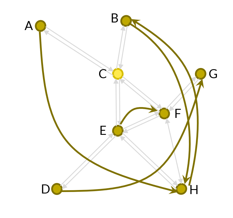 Figure 21: Example demands

|
A-C |
B-C |
C-E |
C-F |
E-H |
F-H |
D-E |
E-F |
F-G |
H-F |
F-C | |
|---|---|---|---|---|---|---|---|---|---|---|---|
| A-H-f1 | 1 | 0 | 1 | 0 | 1 | 0 | 0 | 0 | 0 | 0 | 0 |
| A-H-f2 | 1 | 0 | 0 | 1 | 0 | 1 | 0 | 0 | 0 | 0 | 0 |
| B-H-p1 | 0 | 1 | 1 | 0 | 1 | 0 | 0 | 0 | 0 | 0 | 0 |
| H-B-p1 | 0 | 0 | 0 | 0 | 0 | 0 | 0 | 0 | 0 | 1 | 1 |
| D-G-f1 | 0 | 0 | 0 | 0 | 0 | 0 | 1 | 1 | 1 | 0 | 0 |
| E-F-p1 | 0 | 0 | 0 | 0 | 0 | 0 | 0 | 1 | 0 | 0 | 0 |
| E-F-p2 | 0 | 0 | 0 | 0 | 1 | 0 | 0 | 0 | 0 | 1 | 0 |
| 1 | 2 | 3 | 4 | 5 | 6 | 7 | |
|---|---|---|---|---|---|---|---|
| A-H-f | 2 | 1 | 0 | 0 | 1 | 2 | 0 |
| B-H-p | 0 | 1 | 3 | 2 | 3 | 1 | 0 |
| H-B-p | 0 | 1 | 3 | 2 | 3 | 1 | 0 |
| D-G-f | 3 | 0 | 0 | 0 | 1 | 3 | 0 |
| E-F-p | 0 | 0 | 1 | 1 | 1 | 0 | 0 |
Running this small example in the modeling framework Minizinc [5] with the solver CBC [4] takes less than 1 second, and the result (capacity usage) is shown in table 3. Empty rows does not get any traffic. The objective value is 0.4694.
| 1 | 2 | 3 | 4 | 5 | 6 | 7 | |
|---|---|---|---|---|---|---|---|
| A-C | 1,7 | 1,15 | 0,15 | 0 | 0,85 | 1,2 | 0,95 |
| C-A | |||||||
| B-C | 0 | 0,95 | 2,15 | 2,8 | 2,95 | 1 | 0,15 |
| C-B | 0 | 0,7 | 2,4 | 2,4 | 2,6 | 1,6 | 0,3 |
| C-E | 0 | 0,8 | 2,3 | 2,6 | 2,7 | 1,3 | 0,3 |
| E-C | |||||||
| C-F | 1,05 | 1,48 | 0,48 | 0 | 0,52 | 0,58 | 1,9 |
| F-C | 0 | 0,8 | 2,3 | 2,5 | 2,8 | 1,3 | 0,3 |
| D-E | 2,55 | 0,45 | 0 | 0 | 0,65 | 2,3 | 1.05 |
| E-D | |||||||
| F-G | 1,2 | 1,8 | 0 | 0 | 0,3 | 1,6 | 2,1 |
| G-F | |||||||
| E-F | 1,8 | 1,2 | 0,95 | 1 | 1,25 | 1,7 | 2,1 |
| F-E | |||||||
| E-H | 0 | 0,7 | 2,4 | 2,4 | 2,6 | 1,6 | 0,3 |
| H-E | |||||||
| F-H | 0,4 | 1,8 | 0,8 | 0 | 0,2 | 0,9 | 1,9 |
| H-F | 0 | 0,95 | 2,6 | 2,05 | 3,25 | 0,85 | 0,3 |
If we do a slight change and set the capacity availability on link E-F to 0 during time period 4, simulating e-g- a TCR during that period, we get a new solution with slighter higher objective of 0.48. Since there cannot be any volumes taking the route E-F any longer, the demanded volumes of the traffic E-F previously taking the route E-F-p1 now partially is taking the route E-F-p2 instead which already had volumes for the route E-H-F. If there would have been volumes demanded for D-G-f they would have had to wait somewhere before E (or run slowly) since there is only one named route D-G-f1 for D-G-f. In other words, no named rerouting possibilities have been given since no other route is present in the input data of the example.
![[Uncaptioned image]](2112.09507v1/Example_TrafficRoutes_1.png)
| 1 | 2 | 3 | 4 | 5 | 6 | 7 | |
|---|---|---|---|---|---|---|---|
| A-C | 1,7 | 1,15 | 0,15 | 0 | 0,85 | 1,2 | 0,95 |
| C-A | |||||||
| B-C | 0 | 0,9 | 2,65 | 2,35 | 2,95 | 1 | 0,15 |
| C-B | 0 | 0,7 | 2,4 | 2,3 | 2,7 | 1,65 | 0,25 |
| C-E | 0 | 0,8 | 2,3 | 2,6 | 2,7 | 1,3 | 0,3 |
| E-C | |||||||
| C-F | 1,05 | 1,33 | 0,63 | 0 | 0,38 | 0,72 | 1,9 |
| F-C | 0 | 0,8 | 2,6 | 2 | 2,7 | 1,7 | 0,2 |
| D-E | 2,55 | 0,45 | 0 | 0 | 0,85 | 2,1 | 1,05 |
| E-D | |||||||
| F-G | 0,9 | 2,1 | 0 | 0 | 0,4 | 1,5 | 2,1 |
| G-F | |||||||
| E-F | 1,5 | 1,5 | 0,9 | 0 | 1,65 | 1,35 | 2,1 |
| F-E | |||||||
| E-H | 0 | 0,7 | 2,4 | 3,2 | 2,8 | 1,6 | 0,3 |
| H-E | |||||||
| F-H | 0,4 | 1,65 | 0,95 | 0 | 0,05 | 1,05 | 1,9 |
| H-F | 0 | 0,9 | 2,8 | 2,9 | 2,95 | 1,35 | 0,1 |
| setup | 0 | 0,9 | 0,95 | 0 | 0,05 | 1,05 | 0,1 |
Note that the setup time for changing direction is included in the last row of the table shown in table 4. The example uses the Capacity2_alt2 constraint, with the setup coefficient , therefore the setup time will equal the lower volume value of the two directions. The total capacity used on a single track line is the sum of the volume in both directions plus the setup time, and this sum cannot be larger than the capacity stated, for each time period in the problem.
7.2 Example use of the model
The following example illustrates the use of the model in a real network. The example uses a region around Malm� in Sweden, see figure 22 where the basic network is shown.

The example uses two days of traffic, discretizised into 120 minute periods, and the aim is to see the effect on the traffic over the bridge Malm� (Lernacken, LNK) to Copenhagen (Pepparholmen, PHM, last timetable point in Sweden) when restricting the double track line HIE - M to single track line. The first 6 periods are only to initialize the “pressure” on the system and analogously the last 6 periods are only for “chilling down” all the flows on the different arcs in the network. The middle 12 time periods consists of the actual measure of the impact when restricting the capacity.
The problem is based on the timetable 2020’s traffic and consists of 13 line segments giving 26 directed arcs in the network. There are three different classes of trains: freight trains (FT), intercity trains (IC) and regional trains (RT). In total there are 28 different service types demanded, based on these classes and the origin-destination pairs including different stop patterns of the trains. In total there are 1136 individual demanded trains. In the basic scenario the routes are determined, which gives us 28 TCSs implementing all the demands.
Solving this with the solver CBC, an open source MIP solver, takes about 10 seconds on a standard laptop. No cancellations happen which is expected since this was actual traffic originally planned in the timetable without restricting the capacity.
Now we restrict the capacity to half in both directions on the link HIE-M. Without any rerouting of any trains, 19 trains have to be canceled in total. However, if a rerouting possibility is introduced for the regional trains going PHM-AL and AL-PHM to go round Malm� instead (which is, however, not a preferred route since it is both longer and it involves a direction change at Malm� central station) then all trains in the original traffic can be accomplished but sometimes with longer journey times. Figures 23 and 24 shows the capacity usage over time for the link PHM-LNK and LNK-PHM for the different example runs.


The changes are mostly seen on the link LNK-PHM just after midnight.
This is one intended use of the model, to investigate and do scenario analysis of different rerouting possibilities and measure the impact of them. Experiments have been performed with both scenarios with possessions and restrictions in capacity as well as introductory tests within the Minimum Viable Product 6 in TTR [6] for the case Denmark-Sweden-Norway with the aim to facilitate the construction of a capacity model and capacity supply.
8 Discussion on the time period length
8.1 Extending travel over more than one period
The time period length should is crucial to choose. The smaller it is, the better resolution the model will have. Larger time periods decreases the complexity of the model. A requirement on the time period as the model is formulated in section 5 is that no volume’s traversal time in the investigated network can be larger than the time period length (i.e. it must reach the next node within one time frame):
The reason is that there are no arcs “jumping” or “skipping” the next time period. As can be seen in the figures of section 4.4 the flow is distributed over the direct and next arc, but there are no arc skipping one time period, as would be necessary to have a time period smaller than the traversal time of the modeled trains (again we omit the node inventory arcs, since they only add the possibility to stand still at the station). The difference is highlighted in figure 25.

The model can be extended with additional arcs skipping one or more time periods, shown in figure 26. If this is done, the constraints in the model have to be updated with this extension and the model gets more complex. For instance the capacity constraints has to be extended to cope with all arcs that “uses” (or “touches”) the time period, including the arcs that “flies” over the time period (the trains do travel in the time period, although the “jumping” arc does not start or end within the time period).

8.2 Large departure time windows
Volumes for trains with large departure time windows, larger than one time period, can be modeled to stretch over more than one time period. It is just to distribute the volume over more than one time period. Note however that when doing so in the current model the aggregated volumes must be calculated with the knowledge that the stretch of the volume has a certain form, see figure 27.

Volumes that depart in the second time period must be known to not be distributed over the whole second time period, shown with the blue diagonal border lines for the volumes’ travel along line A-B. The corresponding flow is shown in figure 28.

The aggregation constraints have to be reformulated in order to handle volumes whose time windows stretches over several time periods. Note that this could also be used to narrow the departure time windows and/or the departure times within the time period. care must then be taken, since capacity is only measured as a total amount for the time period as a whole, and the flow model is not handling different capacity usage within the time period. It it therefore essential to choose the time period length in such a way that the model gives a reasonable capacity resolution.
9 Conclusions and future work
We have presented a first description of a railway traffic flow model based on a multi-commodity flow model. the model is innovative in that the model handles volumes of trains rather than scheduling individual trains. The model is also innovative in that time is discretized into time periods and these periods together with the railway network forms the flow model of arcs and nodes. On top of the traffic flow model we introduce two layers, one to handle routes through the network corresponding to Train Service Classes, TSCs [2]. These TSCs package the possible services that can be run in the network. A TSC is a named service from origin to the destination together with important properties such as via stations, axle load, gauge, speed category etc. The TSCs also contain a number (on or more) of named routes through the network. The demand is distributed onto the named routes according to congestion on the route’s line segments and how the objective function is formulated. The idea behind the TSCs is that almost all of the demanded regular traffic on the railway network should fit into declared TSCs. The third layer consist of the demands for traffic, and should be matched on the TSCs to find the best match. this matching also gives the departure time and transport duration which in turn gives the earliest arrival at the destination. Different routes can implement the same demand, thereby giving the route as a decision variable in the model.
All together we have found in these first round of experiments that the model is quite elaborate in terms of understanding the three layered structure but computationally it delivers answers fast. We have tried it with tests up to approximately 20 % of the Swedish railway network and are still able to deliver optimal answers within a couple of minutes. Although these tests are encouraging there are more work to be performed before we could say that the proposed model is ready for use.
The objective function must be developed more carefully. The one presented in this paper is too simple and do not have support in e.g. socio-economic literature or other researched properties. Initial tests with an objective function based on the Priority Criteria formulation of the Swedish Network statement [8] has been performed. It shows promising results and could be an important tool for constructing and evaluating the capacity model, the capacity supply and as a traffic valuation tool when investigating the impact of TCRs.
There are a number improvements to be addressed for the model to be usable in practice. One already mentioned is to formulate the restriction of postponed volumes, to get the demanded train volumes, required to be integer, to depart as an evenly spread volume over time. Of crucial importance is how the capacity properties are formulated so that later timetabling can find a feasible schedule of train individuals along with the proposed volumes from this model. The timetabling complexity is “hidden” in the capacity formulation in the proposed model, in terms of volumes of trains (or capacity units per train type allocated to volumes). We have in this paper sketched how setup times could be introduced in the model, as a function of the heterogeneity of the traffic. Many industry sectors reason in such terms about future production in the early planning phases, i.e. in terms of the number of setups/changes on production facilities when producing different products: how many setups that are needed, the duration of the setup times between different product categories, the impact of longer series of products on intermediate stores, warehouses etc. It is an interesting question in itself if this can be done in railway traffic scheduling, to form feasible high level plans with volumes of traffic usable in e.g. calculating traffic supply and TCR impact in the early phases of the capacity allocation process. The result from these high level plans must have feasible timetables “included” in them, i.e. they must be realizable if this approach shall be used to form a supply of service classes to choose from.
References
- [1] Ravindra Ahuja, Thomas Magnanti and James Orlin “Network Flows: Theory, Algorithms, and Applications” Prentice hall, 1993
- [2] Martin Aronsson “Transporttillgänglighet och tillgänglighetsnyckeltal för järnvägsnät och banunderhåll”, RISE Rapport 2019:33, 2019
- [3] Tomas Liden and Martin Aronsson “An optimization model for renewal scheduling and traffic flow routing” VTI, 2021
- [4] Robin Lougee-Heimer “The Common Optimization INterface for Operations Research” In IBM Journal of Research and Development 47, pp. 57–66
- [5] N Nethercote et al. “MiniZinc: Towards a standard CP modelling language” In Proceedings of the 13th International Conference on Principles and Practice of Constraint Programming, LCNS Springer, 2007 URL: https://www.minizinc.org/
- [6] “Redesign of the International Timetabling Process (TTR)” URL: https://ttr.rne.eu/
- [7] Trafikverket “Analysmetod och samhällsekonomiska kalkylvärden för transportsektorn: ASEK 7.0”, 2020 URL: https://www.trafikverket.se/for-dig-i-branschen/Planera-och-utreda/Planerings--och-analysmetoder/Samhallsekonomisk-analys-och-trafikanalys/gallande-forutsattningar-och-indata/
- [8] Trafikverket “Järnvägsnätsbeskrivning 2021”, Trafikverket Järnvägsnätsbeskrivning, 2021