跳到论文正文
W Papers独立论文阅读器 arXiv:2112.09181 论文正文 计算阅读时间 · 0%
引用这篇论文根据当前论文元数据生成,正式投稿前建议核对。


License: CC BY 4.0
arXiv:2112.09181v2 [cs.LG] 16 Mar 2023

Approximation of functions with one-bit neural networks

C. Sinan Güntürk Note: Courant Institute, New York University. Email: gunturk@cims.nyu.edu    Weilin Li Note: City University of New York, City College. Email: wli6@ccny.cuny.edu
Abstract

The celebrated universal approximation theorems for neural networks roughly state that any reasonable function can be arbitrarily well-approximated by a network whose parameters are appropriately chosen real numbers. This paper examines the approximation capabilities of one-bit neural networks – those whose nonzero parameters are ±a\pm a for some fixed a≠0a\not=0. One of our main theorems shows that for any f∈Cs​([0,1]d)f\in C^{s}([0,1]^{d}) with ‖f‖∞<1\|f\|_{\infty}<1 and error ε\varepsilon, there is a fN​Nf_{NN} such that |f⁡(𝒙)−fN​N​(𝒙)|≤ε|f(\boldsymbol{x})-f_{NN}(\boldsymbol{x})|\leq\varepsilon for all 𝒙\boldsymbol{x} away from the boundary of [0,1]d[0,1]^{d}, and fN​Nf_{NN} is either implementable by a {±1}\{\pm 1\} quadratic network with O(ε−2d/s)O(\varepsilon^{-2d/s}) parameters or a {±12}\{\pm\frac{1}{2}\} ReLU network with O(ε−2d/slog(1/ε))O(\varepsilon^{-2d/s}\log(1/\varepsilon)) parameters, as ε→0\varepsilon\to 0. We establish new approximation results for iterated multivariate Bernstein operators, error estimates for noise-shaping quantization on the Bernstein basis, and novel implementation of the Bernstein polynomials by one-bit quadratic and ReLU neural networks.

Keywords: neural network, quantization, one-bit, Bernstein, polynomial approximation

MSC2020: 41A10, 41A25, 41A36, 41A63, 42C15, 68T07

1 Introduction

1.1 Motivation

In this paper, we address the following question regarding the approximation capabilities of quantized neural networks: what classes of functions can be approximated by neural networks of a given size such that their weights and biases are constrained to be in a small set of allowable values, especially with regards to the extreme one-bit case? While this is an interesting mathematical question by itself and warrants special attention given the growing importance of machine learning across numerous scientific disciplines, here we illuminate two particularly important broader questions that motivate this theoretical study.

Our first motivation comes from a practical problem. State-of-the-art neural networks oftentimes contain a massive number of parameters and are trained on enormous computational machines. It appears that in regards to performance of neural networks, the “bigger is better” philosophy largely holds true [7]. As higher resolution audio, image, and video data become increasingly more common, the size of high performance networks will only continue to grow and require more computational resources to utilize. This conflicts with the desire to use them on portable and low power devices such as smartphones. Quantization is the process of replacing high resolution floating point numbers with coarser ones. It is a natural solution to this issue, since simpler binary operations can help alleviate the costly computational burden that comes with using expensive floating point operations.

Our second motivation is related to the over-parameterization phenomena. Since state-of-the-art neural networks often contain many more parameters than both the number of training samples and data dimensionality [5], it is widely believed that there is not a unique set of parameters that can be used to represent a given function. If we imagine that the set of all parameters generating a prescribed function is a manifold embedded in a high dimensional parameter space, then our main question is closely related to whether this manifold is sufficiently close to some lattice point. Since certain parameter choices may be more desirable than others, this is a central question in not only quantization, but also in neural network compression and model reduction.

1.2 Quantized neural networks

In this paper, we exclusively examine strict neural networks. We use the adjective “strict” to emphasize that such networks do not have any skip connections and apply the same activation function to each node except for the final affine layer. More specifically, fix a function β:ℝ→ℝ\beta\colon\mathbb{R}\to\mathbb{R}, and slightly abusing notation, for each m≥1m\geq 1, we extend it to a map β:ℝm→ℝm\beta\colon\mathbb{R}^{m}\to\mathbb{R}^{m} defined as β⁡(𝒙):=(β⁡(x1),…,β⁡(xm))\beta(\boldsymbol{x}):=(\beta(x_{1}),\dots,\beta(x_{m})).

Definition 1.1.

A strict neural network with activation β\beta is any function f:ℝd→ℝmf\colon\mathbb{R}^{d}\to\mathbb{R}^{m} of the form,

f(𝒙):=WLβ(WL−1⋯β(W1(𝒙))),Wℓ(𝒖):=Aℓ𝒖+𝒃ℓforℓ=1,…,L.f(\boldsymbol{x}):=W_{L}\beta(W_{L-1}\cdots\beta(W_{1}(\boldsymbol{x}))),\quad W_{\ell}(\boldsymbol{u}):=A_{\ell}\boldsymbol{u}+\boldsymbol{b}_{\ell}\quad\text{for}\quad\ell=1,\dots,L.

In this definition, each Aℓ∈ℝNℓ×Nℓ−1A_{\ell}\in\mathbb{R}^{N_{\ell}\times N_{\ell-1}} is referred to as a weight matrix, 𝒃ℓ∈ℝNℓ\boldsymbol{b}_{\ell}\in\mathbb{R}^{N_{\ell}} is called a bias vector, LL is the number of layers, and N0=dN_{0}=d and NL=mN_{L}=m. For each 1≤ℓ≤L−11\leq\ell\leq L-1, we refer to 𝒖ℓ:=β(Wℓβ(⋯β(W1(𝒙)))\boldsymbol{u}_{\ell}:=\beta(W_{\ell}\beta(\cdots\beta(W_{1}(\boldsymbol{x}))) as the ℓ\ell-th layer’s output. This network has LL layers, and applies the same activation function to each node except for the final linear layer. It has NℓN_{\ell} nodes in layer ℓ\ell, hence has ∑ℓ=1LNℓ\sum_{\ell=1}^{L}N_{\ell} nodes in total, and we define the number of parameters as however many nonzero entries in {Aℓ}ℓ=1L\{A_{\ell}\}_{\ell=1}^{L} and {𝒃ℓ}ℓ=1L\{\boldsymbol{b}_{\ell}\}_{\ell=1}^{L} there are. Since we place no restrictions on the weight matrices’ structures, our framework allows for fully connected and convolutional networks. We say a function gg can be implemented by neural network provided it can be written in the above form with appropriate weights.

Other common definitions of a neural network allow for additional operations and flexibility. For instance, some conventions allow for the use of skip connections whereby 𝒖ℓ+1\boldsymbol{u}_{\ell+1} is allowed to depend on any previous layer’s outputs 𝒖ℓ,…,𝒖1\boldsymbol{u}_{\ell},\dots,\boldsymbol{u}_{1}. Another example is the use of different activation functions per node and possibly in each layer, including the identity function which effectively bypasses an activation. Following the terminology from [19], to differentiate between the strict notion we use versus less stringent notions, we refer to the latter as generalized neural networks.

We are interested in strict quantized neural networks. While it is convenient to treat the entries of {Aℓ}ℓ=1L\{A_{\ell}\}_{\ell=1}^{L} and {𝒃ℓ}ℓ=1L\{\boldsymbol{b}_{\ell}\}_{\ell=1}^{L} as real numbers for theoretical analysis, when used for computations, each entry is traditionally stored as a 32-bit float in memory. To reduce the number of bits, we consider a fixed finite 𝒜⊆ℝ\mathcal{A}\subseteq\mathbb{R} called the alphabet.

Definition 1.2.

A strict 𝒜\mathcal{A}-quantized neural network is a strict neural network where all nonzero entries of the weight matrices {Aℓ}ℓ=1L\{A_{\ell}\}_{\ell=1}^{L} and bias vectors {𝒃ℓ}ℓ=1L\{\boldsymbol{b}_{\ell}\}_{\ell=1}^{L} belong to 𝒜\mathcal{A}.

An alphabet 𝒜\mathcal{A} that only consists of a small set of allowable values, such as the extreme one-bit case, is theoretically interesting as it poses stringent constraints and is computationally relevant as one can take advantage of special hardware and software for one-bit floating point operations. Since the weights and biases are selected from the same alphabet 𝒜\mathcal{A}, this definition imposes a particular scaling on the associated network, which can be altered by dilating the domain.

1.3 The challenge: approximation by coarsely quantized networks

The problem of neural network quantization can be studied from an approximation theory perspective. Let 𝒩:=𝒩⁡(𝒜,β,L,N,P)\mathcal{N}:=\mathcal{N}(\mathcal{A},\beta,L,N,P) be the set of functions that can be expressed as a strict 𝒜\mathcal{A}-quantized neural network with activation β\beta and has at most LL layers, NN nodes, and PP parameters. For a prescribed function class ℱ\mathcal{F}, and distortion measure ℰ:ℱ×𝒩→ℝ\mathcal{E}\colon\mathcal{F}\times\mathcal{N}\to\mathbb{R}, we study the

approximation error:=supf∈ℱinfg∈𝒩ℰ⁡(f,g).\text{approximation error}\quad:=\quad\sup_{f\in\mathcal{F}}\ \ \inf_{g\in\mathcal{N}}\ \ \mathcal{E}(f,g).

The approximation error achieved by generalized neural networks has been extensively studied in the traditional case where there is no quantization. Well known classical universal approximation theorems [10, 3] are qualitative statements for shallow networks. Modern versions [39, 34, 30, 12, 19] provide quantitative approximation rates in terms of the function class, number of layers, parameters, etc. This is only a partial list of references, and additional ones can be found in the bibliography of a recent comprehensive survey [13]. Perhaps this is a suitable place to mention that the set of strict neural networks is a subset of their generalized counterparts, so any function class that can be approximated by strict quantized neural networks can also be well-approximated by generalized unquantized ones.

It is natural to wonder if these results or their proof strategies can be adapted to strict quantized networks. If 𝒜\mathcal{A} is of sufficiently high resolution and covers a wide range of numbers, such as 𝒜=δ​ℤ∩[−M,M]\mathcal{A}=\delta\mathbb{Z}\cap[-M,M], for sufficiently large MM and small δ>0\delta>0, then the aforementioned approximation results for unquantized generalized networks can be suitably adapted, such as in [6, Lemma 3.7]. However, this approach requires using an increasingly higher resolution alphabet (reducing δ\delta) to achieve smaller errors. Major difficulties come into play once we fix an alphabet 𝒜\mathcal{A} and a function class ℱ\mathcal{F}, and ask to approximate any f∈ℱf\in\mathcal{F} up to any error ε\varepsilon by a 𝒜\mathcal{A}-quantized strict neural network.

Many of the aforementioned papers employ the following ubiquitous strategy. For a prescribed f∈ℱf\in\mathcal{F}, we approximate ff by a particular linear combination, ∑k=1Nak​ϕk\sum_{k=1}^{N}a_{k}\phi_{k}, where the coefficients {ak}k=1N\{a_{k}\}_{k=1}^{N} depend on ff and the span of {ϕk}k=1∞\{\phi_{k}\}_{k=1}^{\infty} is dense in ℱ\mathcal{F}. Examples of {ϕk}k=1∞\{\phi_{k}\}_{k=1}^{\infty} include local polynomials, ridge functions, and wavelets. While it is possible that ϕk\phi_{k} is not implementable as a generalized neural network, it is enough to find a ψk\psi_{k} that is a close approximation of ϕk\phi_{k} which is implementable. After {ψk}k=1N\{\psi_{k}\}_{k=1}^{N} are implemented, the summation ∑k=1Nak​ψk\sum_{k=1}^{N}a_{k}\psi_{k} is carried out by a linear last layer whose weights are {ak}k=1N\{a_{k}\}_{k=1}^{N}.

However, this approximation and implementation strategy becomes problematic when 𝒜\mathcal{A} is a small set, especially for the one-bit case. For example, if we were to closely follow the same strategy, we need each ψk\psi_{k} to be implementable by a 𝒜\mathcal{A}-quantized strict neural network, and require ak∈𝒜a_{k}\in\mathcal{A} to perform the linear combination ∑k=1Nak​ψk\sum_{k=1}^{N}a_{k}\psi_{k}. From this point of view, it is natural to desire the following three properties:

  1. (P1P_{1})

    Approximation. Given a large function class ℱ\mathcal{F}, finite linear combinations of {ϕk}k=1∞\{\phi_{k}\}_{k=1}^{\infty} with real coefficients can efficiently approximate any f∈ℱf\in\mathcal{F}.

  2. (P2P_{2})

    Quantization. For any f∈ℱf\in\mathcal{F} and its approximation ∑k=1Nak​ϕk\sum_{k=1}^{N}a_{k}\phi_{k}, the real coefficients {ak}k=1N\{a_{k}\}_{k=1}^{N} can be replaced with suitable ones from just 𝒜\mathcal{A} without incurring to much additional error.

  3. (P3P_{3})

    Implementation. For each ϕk\phi_{k}, there is a good approximant ψk\psi_{k} that can be implemented by a strict 𝒜\mathcal{A}-quantized neural network.

While there many satisfactory choices for (P1P_{1}), it is not immediate if any of those can be made compatible with (P2P_{2}) and (P3P_{3}). On the other hand, there are a few known choices of {ϕk}k=1∞\{\phi_{k}\}_{k=1}^{\infty} that satisfy (P2P_{2}). Some are for very restrictive function classes: when ff is bandlimited and {ϕk}k=1∞\{\phi_{k}\}_{k=1}^{\infty} contain shifts of a sinc-kernel [11, 20] or when ff is a power series of a single complex variable and {ϕk}k=1∞\{\phi_{k}\}_{k=1}^{\infty} is the standard polynomial power basis [21].

The approach taken in this paper builds upon our recent publication [22], and there, we showed that any continuous function on [0,1][0,1] can be approximated by a ±1\pm 1 linear combination of Bernstein polynomials. A Bernstein polynomial of order nn and index 𝒌=(k1,…,kd)\boldsymbol{k}=(k_{1},\dots,k_{d}) with 0≤kℓ≤n0\leq k_{\ell}\leq n is the function pn,𝒌:ℝd→[0,1]p_{n,\boldsymbol{k}}\colon\mathbb{R}^{d}\to[0,1] defined as

pn,𝒌​(𝒙)=(n𝒌)​𝒙𝒌​(1−𝒙)n−𝒌=∏ℓ=1d(nkℓ)​xℓkℓ​(1−xℓ)n−kℓ.p_{n,\boldsymbol{k}}(\boldsymbol{x})=\binom{n}{\boldsymbol{k}}\boldsymbol{x}^{\boldsymbol{k}}(1-\boldsymbol{x})^{n-\boldsymbol{k}}=\prod_{\ell=1}^{d}\binom{n}{k_{\ell}}x_{\ell}^{k_{\ell}}(1-x_{\ell})^{n-k_{\ell}}.

Continuing with this line of research, we investigate the multivariate Bernstein system as a potential candidate that satisfies all three of our desired properties.

1.4 Main contributions

The main theorems are proved by decomposing the total approximation error into three Bernstein related terms,

f−fN​N=f−fB⏟Bern. approx. error+fB−fQ⏟Bern. quan. error+fQ−fN​N⏟Bern. implementation error.f-f_{NN}\quad=\underbrace{f-f_{B}}_{\text{Bern. approx. error}}+\underbrace{f_{B}-f_{Q}}_{\text{Bern. quan. error}}+\underbrace{f_{Q}-f_{NN}}_{\text{Bern. implementation error}}.

Here, fBf_{B} is a linear combination of multivariate Bernstein polynomials whose coefficients are real and appropriately bounded, fQf_{Q} is a ±a\pm a linear combination of multivariate Bernstein polynomials for appropriate aa, and fN​Nf_{NN} is a function implementable by a strict {±a}\{\pm a\}-quantized neural network.

Our first main theorem concerns f−fQ=(f−fB)+(fB−fQ)f-f_{Q}=(f-f_{B})+(f_{B}-f_{Q}). It shows that any smooth multivariate ff can be approximated by a ±1\pm 1 linear combination of Bernstein polynomials with a quantitative rate that exploits smoothness of ff. In the following, ∥⋅∥Cs\|\cdot\|_{C^{s}} is a norm on the space of ss-times continuously differentiable functions and ∥⋅∥C1​Lip\|\cdot\|_{C^{1}{\rm Lip}} is a norm on the space of continuously differentiable functions whose first order partial derivatives are Lipschitz.

Theorem A.

Let s,d,n≥1s,d,n\geq 1, μ∈(0,1)\mu\in(0,1), and f∈Cs​([0,1]d)f\in C^{s}([0,1]^{d}) with ‖f‖∞≤μ\|f\|_{\infty}\leq\mu. If s≥3s\geq 3, also assume that n≥2s+1​d4​(1−μ)​‖f‖C1​Lip.n\geq\displaystyle\frac{\sqrt{2^{s+1}}d}{4(1-\mu)}\|f\|_{C^{1}{\rm Lip}}. Then for any 1≤ℓ≤d1\leq\ell\leq d, there exists a sequence {σ𝒌}0≤𝒌≤n\{\sigma_{\boldsymbol{k}}\}_{0\leq\boldsymbol{k}\leq n} such that σ𝒌∈{±1}\sigma_{\boldsymbol{k}}\in\{\pm 1\} for each 𝒌\boldsymbol{k} and for all 𝒙∈[0,1]d\boldsymbol{x}\in[0,1]^{d},

|f(𝒙)−∑0≤𝒌≤nσ𝒌pn,𝒌(𝒙)|≲s,d,μ∥f∥Csmin(1,n−s/2xℓ−s(1−xℓ)−s).\Big|f(\boldsymbol{x})-\sum_{0\leq\boldsymbol{k}\leq n}\sigma_{\boldsymbol{k}}p_{n,\boldsymbol{k}}(\boldsymbol{x})\Big|\lesssim_{s,d,\mu}\|f\|_{C^{s}}\min\big(1,n^{-s/2}x_{\ell}^{-s}(1-x_{\ell})^{-s}\big).

A is proved constructively by first approximating ff with a suitable fBf_{B} of the form ∑0≤𝒌≤na𝒌​pn,𝒌\sum_{0\leq\boldsymbol{k}\leq n}a_{\boldsymbol{k}}p_{n,\boldsymbol{k}}. Then secondly, the coefficients {a𝒌}0≤𝒌≤n\{a_{\boldsymbol{k}}\}_{0\leq\boldsymbol{k}\leq n} are fed into an algorithm called Σ​Δ\Sigma\Delta quantization to produce the desired one-bit sequence {σ𝒌}0≤𝒌≤n\{\sigma_{\boldsymbol{k}}\}_{0\leq\boldsymbol{k}\leq n} from which we get fQf_{Q} of the form ∑0≤𝒌≤nσ𝒌​pn,𝒌\sum_{0\leq\boldsymbol{k}\leq n}\sigma_{\boldsymbol{k}}p_{n,\boldsymbol{k}}. The approximant fQf_{Q} is a ±1\pm 1 linear combination of Bernstein polynomials and can be numerically computed, provided that we have point samples of ff on a sufficiently dense grid, as summarized in Algorithm 1. The Σ​Δ\Sigma\Delta algorithm falls under a general class of “noise-shaping” methods, where the main idea is to compute the signs {σ𝒌}0≤𝒌≤n\{\sigma_{\boldsymbol{k}}\}_{0\leq\boldsymbol{k}\leq n} so that the “noise” {a𝒌−σ𝒌}0≤𝒌≤n\{a_{\boldsymbol{k}}-\sigma_{\boldsymbol{k}}\}_{0\leq\boldsymbol{k}\leq n}, when fed into the synthesis operator c↦∑0≤𝒌≤nc𝒌​pn,𝒌c\mapsto\sum_{0\leq\boldsymbol{k}\leq n}c_{\boldsymbol{k}}p_{n,\boldsymbol{k}}, is small in a suitable sense.

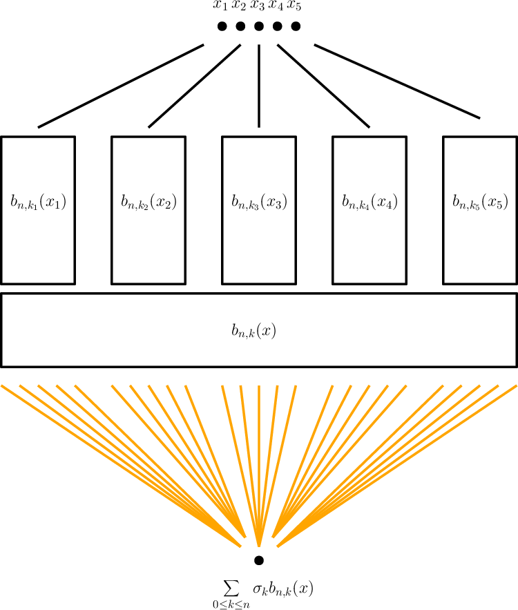
Our second main result deals with the implementation error fQ−fN​Nf_{Q}-f_{NN}. It shows that any one-bit linear combination of Bernstein polynomials is implementable by strict one-bit neural networks, with either the quadratic ρ⁡(t)=12​t2\rho(t)=\frac{1}{2}t^{2} or ReLU σ⁡(t)=max⁡(t,0)\sigma(t)=\max(t,0) activation. The proof is constructive and schematic diagrams for the constructed networks are shown in Figures 1(a) and 1(b).

Theorem B.

For any integers d,n≥1d,n\geq 1 and function f=∑0≤𝒌≤nσ𝒌​pn,𝒌f=\sum_{0\leq\boldsymbol{k}\leq n}\sigma_{\boldsymbol{k}}p_{n,\boldsymbol{k}} where σ𝒌∈{±1}\sigma_{\boldsymbol{k}}\in\{\pm 1\} for each 𝒌\boldsymbol{k}, the following hold.

  • •

    There is a {±1}\{\pm 1\}-quantized quadratic neural network fN​N,ρf_{NN,\rho} that has O⁡(n)O(n) layers and O⁡(nd)O(n^{d}) nodes and parameters, as n→∞n\to\infty, such that fN​N,ρ=ff_{NN,\rho}=f.

  • •

    For each ε\varepsilon, there exists a {±12}\{\pm\frac{1}{2}\}-quantized ReLU neural network fN​N,σf_{NN,\sigma} with O⁡(n​log⁡(n/ε))O(n\log(n/\varepsilon)) layers and O⁡((n2+nd)​log⁡(n/ε))O((n^{2}+n^{d})\log(n/\varepsilon)) nodes and parameters, as n→∞n\to\infty and ε→0\varepsilon\to 0, such that ‖f−fN​N,σ‖∞≤ε\|f-f_{NN,\sigma}\|_{\infty}\leq\varepsilon.

Combining the previous theorems, we obtain the final main theorem of this paper.

Theorem C.

Let s,d,n≥1s,d,n\geq 1, μ∈(0,1)\mu\in(0,1), and f∈Cs​([0,1]d)f\in C^{s}([0,1]^{d}) with ‖f‖∞≤μ\|f\|_{\infty}\leq\mu. If s≥3s\geq 3, also assume that n≥2s+1​d4​(1−μ)​‖f‖C1​Lip.n\geq\displaystyle\frac{\sqrt{2^{s+1}}d}{4(1-\mu)}\|f\|_{C^{1}{\rm Lip}}. For any 1≤ℓ≤d1\leq\ell\leq d, there exist functions fN​N,ρf_{NN,\rho} and fN​N,σf_{NN,\sigma} such that:

  • •

    for fN​N∈{fN​N,ρ,fN​N,σ}f_{NN}\in\{f_{NN,\rho},f_{NN,\sigma}\} and any 𝒙∈[0,1]d\boldsymbol{x}\in[0,1]^{d},

    |f(𝒙)−fN​N(𝒙)|≲s,d,μ∥f∥Csmin(1,n−s/2xℓ−s(1−xℓ)−s).|f(\boldsymbol{x})-f_{NN}(\boldsymbol{x})|\lesssim_{s,d,\mu}\|f\|_{C^{s}}\min\big(1,n^{-s/2}x_{\ell}^{-s}(1-x_{\ell})^{-s}\big).
  • •

    fN​N,ρf_{NN,\rho} is implementable by a strict {±1}\{\pm 1\}-quantized quadratic neural network that has O⁡(n)O(n) layers and O⁡(nd)O(n^{d}) nodes and parameters, as n→∞n\to\infty.

  • •

    fN​N,σf_{NN,\sigma} is implementable by a strict {±12}\{\pm\frac{1}{2}\}-quantized ReLU neural network that has O⁡(n​log⁡n)O(n\log n) layers and O⁡((n2+nd)​log⁡n)O((n^{2}+n^{d})\log n) nodes and parameters, as n→∞n\to\infty.

Refer to caption
(a) One-bit Bernstein neural network
Refer to caption
(b) Pascal-Bernstein triangle
Figure 1: Schematic diagrams of the constructed one-bit neural networks.

1.5 Why Bernstein? Other contributions

In this paper, we show that the multivariate Bernstein polynomials {pn,𝒌}0≤𝒌≤n\{p_{n,\boldsymbol{k}}\}_{0\leq\boldsymbol{k}\leq n} of order nn satisfy the three important properties (P1P_{1}), (P2P_{2}), and (P3P_{3}), which are then used to prove the main theorems.

  1. (P1P_{1})

    Approximation. In Theorem 2.4, we use iterated Bernstein operators to approximate any f∈Cs​([0,1]d)f\in C^{s}([0,1]^{d}), with a rate of approximation that exploits smoothness of ff, which generalizes the one-dimensional results of Micchelli [32] and Felbecker [16]. This allows us to avoid a known saturation result [14, Chapter 10, Theorem 3.1], which says that the usual Bernstein operator is unable to exploit higher order derivatives of the target function. In Theorem 2.6, we convert the resulting iterated approximant into a linear combination of Bernstein polynomials without much amplification in the resulting coefficients.

  2. (P2P_{2})

    Quantization. In Theorem 3.5, we show that any linear combination of Bernstein polynomials with real coefficients can be replaced with a suitable sequence of ±1\pm 1 linear combination, without significant error. This step is done constructively through a directional Σ​Δ\Sigma\Delta algorithm. This is perhaps surprising because previous applications of noise-shaping quantization utilize some notion of redundancy in the generating system, whereas the Bernstein polynomials are linearly independent. One explanation is that the Bernstein system of order nn and of a single variable span a subspace whose numerical rank is approximately n\sqrt{n}.

  3. (P3P_{3})

    Implementation. For both the ReLU and quadratic activation functions, our implementation strategy exploits a natural Pascal triangle interpretation of the univariate Bernstein polynomials, as shown in Figure 1(b). This connection is vital in being able to implement the Bernstein polynomials in a stable and efficient way. Since we exclusively employ strict neural networks, our constructions are more constrained than those found in papers that employ generalized neural networks. The constructions are found in A.

1.6 Additional related work

This paper addresses the universal approximation capabilities of coarsely quantized neural networks: whether they can arbitrarily well-approximate large function classes. Related work on approximation by unquantized neural networks or with variable high resolution alphabets were discussed in Section 1.3. There we also explain why the problem of universal approximation with coarsely quantized networks is significantly different and requires novel technical developments.

On the other hand, several algorithms for neural network quantization have been developed and their performances have been evaluated empirically, see the survey article [25]. In essence, existing algorithms take a pre-trained network and replace each layer with a quantized approximant, and/or directly train the network by quantizing the back-propagation vectors. While it has been empirically observed that they can compress networks without sacrificing substantial accuracy, there is little theory explaining why. Several recent works [2, 31] address this gap by proposing gradient-based quantization methods with provable guarantees.

This paper’s material builds upon our previous work [23]. There we analyzed the approximation properties of one-bit linear combinations of univariate Bernstein polynomials, and Theorem C is a multivariate generalization of [23, Theorem 7]. While [23, Appendix B] briefly touches upon implementation by quadratic neural networks, it only pertained to a single dimension and did not provide quantitative bounds for the size of such networks. On the other hand, the results in this paper deal with arbitrary dimensions, and for both the quadratic and ReLU activation functions.

This version improves upon the first draft of this paper in two ways: we implement the approximation strategy given in A with strict neural networks, and the ReLU case only necessitates a one-bit alphabet.

1.7 Organization

The organization of subsequent sections follow the ordering (P1P_{1}), (P2P_{2}), and (P3P_{3}). The Bernstein approximation error f−fBf-f_{B} is treated in Section 2. The quantization error in the Bernstein basis fB−fQf_{B}-f_{Q} is dealt with in Section 3. The implementation error of these one-bit approximations fQ−fN​Nf_{Q}-f_{NN} for both the quadratic and ReLU activation functions is studied in Section 4, while the constructions of fN​Nf_{NN} are carried out in Appendix A. Proofs of Theorems A, B, and C are provided in Sections 3.4, 4.3, and 4.4, respectively. Final remarks and other aspects of this paper, including the computational method and entropy considerations, are contained in Section 5.

1.8 Basic notation

We let ℝ\mathbb{R} be the reals and ℕ\mathbb{N} be the natural numbers including zero. For reasons that will become evident, we let log\log denote the base 2 logarithm. The ceiling and floor functions are denoted ⌈⋅⌉\lceil\cdot\rceil and ⌊⋅⌋\lfloor\cdot\rfloor, respectively. We use the notation A≲BA\lesssim B to mean that there is a universal constant CC such that A≤C​BA\leq CB. When we write A≲a,b,cBA\lesssim_{a,b,c}B, we mean that there is a C>0C>0 that possibly depends on a,b,ca,b,c for which A≤C​BA\leq CB.

Let 𝒆1,…,𝒆d\boldsymbol{e}_{1},\dots,\boldsymbol{e}_{d} denote the canonical orthonormal basis for ℝd\mathbb{R}^{d}. For any p∈[1,∞]p\in[1,\infty], let ∥⋅∥p\|\cdot\|_{p} be the usual pp-th norm on vectors in ℝd\mathbb{R}^{d}. We also use the same notation for the ℓp\ell^{p}-norm of a function defined on a countable set, and the LpL^{p} norm of a function.

We denote multi-indices and tuples with boldface letters. For 𝒌,ℓ∈ℕd\boldsymbol{k},\boldsymbol{\ell}\in\mathbb{N}^{d} and m∈ℕm\in\mathbb{N}, we define the following. We write 𝒌≤ℓ\boldsymbol{k}\leq\boldsymbol{\ell} as shorthand for kj≤ℓjk_{j}\leq\ell_{j} for each jj. Likewise, we let 𝒌≤m\boldsymbol{k}\leq m (or m≤𝒌m\leq\boldsymbol{k}) to mean that kj≤mk_{j}\leq m (or m≤kjm\leq k_{j}) for each jj. For any 𝒙∈ℝd\boldsymbol{x}\in\mathbb{R}^{d}, let 𝒙𝒌:=x1k1⋯xdkd\boldsymbol{x}^{\boldsymbol{k}}:=x_{1}^{k_{1}}\cdots x_{d}^{k_{d}}, and |𝒌|=k1+⋯+kd|\boldsymbol{k}|=k_{1}+\cdots+k_{d}. The degree of 𝒙𝒌\boldsymbol{x}^{\boldsymbol{k}} is defined to be |𝒌||\boldsymbol{k}|. For any t∈ℝt\in\mathbb{R}, we let t​𝒌=(t​k1,…,t​kd)t\boldsymbol{k}=(tk_{1},\dots,tk_{d}). We follow standard convention for dealing with combinatorial factors:

(𝒌ℓ):=∏j=1d(kjℓj),and(m𝒌):=∏j=1d(mkj).\binom{\boldsymbol{k}}{\boldsymbol{\ell}}:=\prod_{j=1}^{d}\binom{k_{j}}{\ell_{j}},\quad\text{and}\quad\binom{m}{\boldsymbol{k}}:=\prod_{j=1}^{d}\binom{m}{k_{j}}.

2 Approximation error

In this section, we concentrate on the error incurred by approximating a smooth ff with fB=∑0≤𝒌≤na𝒌​pn,𝒌f_{B}=\sum_{0\leq\boldsymbol{k}\leq n}a_{\boldsymbol{k}}p_{n,\boldsymbol{k}}, a linear combination of Bernstein polynomials of order nn, where each coefficient a𝒌a_{\boldsymbol{k}} can be suitably controlled in terms of ff. For reasons that will become apparent later on when we discuss the quantization error, we will construct a fBf_{B} whose coefficients in the Bernstein basis are not much larger than ‖f‖∞\|f\|_{\infty}. More specifically, the results of this section will provide us with upper bounds on the approximation error by Bernstein polynomials,

ℰn,capprox​(f):=inf{a𝒌}0≤𝒌≤n,|a𝒌|≤c‖f−∑0≤𝒌≤na𝒌​pn,𝒌‖∞.\mathcal{E}_{n,c}^{\text{approx}}(f):=\inf_{\{a_{\boldsymbol{k}}\}_{0\leq\boldsymbol{k}\leq n},\,|a_{\boldsymbol{k}}|\leq c}\Big\|f-\sum_{0\leq\boldsymbol{k}\leq n}a_{\boldsymbol{k}}p_{n,\boldsymbol{k}}\Big\|_{\infty}.

A famous theorem of Bernstein showed that Bn​(f)B_{n}(f) converges uniformly to ff on [0,1][0,1] provided that ff is continuous, which generalizes to higher dimensions, see [27] for the two-dimensional case. While Bn​(f)B_{n}(f) may appear to be a natural candidate for fBf_{B}, there is a well known saturation result which says that, even for infinitely differentiable ff, the fastest rate of decay is 1/n1/n, see [14, Chapter 10, Theorem 3.1].

To circumvent this saturation, we follow an approach of Micchelli [32], and show in Theorem 2.4, that appropriate iterates of multivariate Bernstein operators achieve improved convergence rates that exploit smoothness of ff. Theorem 2.5 allows us to convert these iterated approximations to a linear combination of Bernstein polynomials and Theorem 2.6 provides us with the existence of a suitable fBf_{B}.

2.1 Background on Bernstein polynomials

For a fixed integer n≥1n\geq 1, we denote the set of univariate Bernstein polynomials by ℬn:={pn,k}k=0n\mathcal{B}_{n}:=\{p_{n,k}\}_{k=0}^{n}. Each pn,k:[0,1]→[0,1]p_{n,k}\colon[0,1]\to[0,1] is a polynomial of degree nn and

pn,k​(x):=(nk)​xk​(1−x)n−k.p_{n,k}(x):=\binom{n}{k}x^{k}(1-x)^{n-k}.

The Bernstein polynomials are nonnegative, form a partition of unity for [0,1][0,1], and form a basis for the vector space of nn degree algebraic polynomials. They can be used to give a constructive proof of the classical Weierstrass theorem, by showing that any continuous ff on [0,1][0,1] can be uniformly approximated by the Bernstein polynomial of ff,

Bn​(f)​(x):=∑k=0nf⁡(kn)​pn,k​(x).B_{n}(f)(x):=\sum_{k=0}^{n}f\Big(\frac{k}{n}\Big)p_{n,k}(x).

For reasons that will be apparent later, it will be convenient for us to extend the index kk beyond nn in the definition of pn,kp_{n,k}. If k<0k<0 or k>nk>n, then we define pn,k:=0p_{n,k}:=0.

The Bernstein polynomials can also be viewed from a probabilistic perspective. For any x∈[0,1]x\in[0,1], the quantity pn,k​(x)p_{n,k}(x) is the probability that kk successes occur in nn independent Bernoulli trials each with probability of success xx. Since the expected value is n​xnx, for each integer s≥0s\geq 0, the ss-th central moment is

Tn,s​(x):=∑k=0n(k−n​x)s​pn,k​(x).T_{n,s}(x):=\sum_{k=0}^{n}(k-nx)^{s}p_{n,k}(x).

It is known that Tn,sT_{n,s} is a polynomial in xx of degree at most ss and in nn of degree at most ⌊s/2⌋\lfloor s/2\rfloor. We will employ a few specific formulas for small ss. For each x∈[0,1]x\in[0,1], with the short hand notation X:=x⁡(1−x)X:=x(1-x), we have

Tn,0(x)=1,Tn,1(x)=0,Tn,2(x)=nX,Tn,3(x)=n(1−2x)X,Tn,4(x)=3n2X2+n(X−6X2).\begin{split}&T_{n,0}(x)=1,\quad T_{n,1}(x)=0,\quad T_{n,2}(x)=nX,\\ &T_{n,3}(x)=n(1-2x)X,\quad T_{n,4}(x)=3n^{2}X^{2}+n(X-6X^{2}).\end{split} (2.1)

For each integer s≥0s\geq 0, there is a constant AsA_{s} such that for all n≥1n\geq 1 and x∈[0,1]x\in[0,1], we have

0≤Tn,2​s​(x)≤As​ns.0\leq T_{n,2s}(x)\leq A_{s}n^{s}. (2.2)

See [14, Chapter 10] for proofs of the above results. Although we will not need explicit upper bounds for AsA_{s}, some can be found in [1, 33].

For dimension d≥1d\geq 1 and integer n≥1n\geq 1, Bernstein polynomials are defined to be tensor products of single variable Bernstein polynomials.

Definition 2.1.

The multivariate Bernstein polynomials of order nn is ℬn:={pn,𝒌}0≤𝒌≤n\mathcal{B}_{n}:=\{p_{n,\boldsymbol{k}}\}_{0\leq\boldsymbol{k}\leq n}, where each pn,𝒌:[0,1]d→[0,1]p_{n,\boldsymbol{k}}\colon[0,1]^{d}\to[0,1] is defined as,

pn,𝒌(𝒙):=pn,k1(x1)⋯pn,kd(xd)=(n𝒌)𝒙𝒌(1−𝒙)n−𝒌.p_{n,\boldsymbol{k}}(\boldsymbol{x}):=p_{n,k_{1}}(x_{1})\cdots p_{n,k_{d}}(x_{d})=\binom{n}{\boldsymbol{k}}\boldsymbol{x}^{\boldsymbol{k}}(1-\boldsymbol{x})^{n-\boldsymbol{k}}.

Whenever there is a 1≤ℓ≤d1\leq\ell\leq d such that either kℓ<0k_{\ell}<0 or kℓ>nk_{\ell}>n, then we define pn,𝒌=0p_{n,\boldsymbol{k}}=0. It is important to mention that we exclusively use multivariate Bernstein polynomials that are formed as tensor products. They are significantly different from Bernstein polynomials on the canonical dd-dimensional simplex.

Several properties of multivariate Bernstein polynomials can be deduced by exploiting their tensor product structure. They form a partition of unity for [0,1]d[0,1]^{d}, and in particular,

∑kℓ=0npn,kℓ​(xℓ)=1for all1≤ℓ≤dand𝒙∈[0,1]d.\sum_{k_{\ell}=0}^{n}p_{n,k_{\ell}}(x_{\ell})=1\quad\text{for all}\quad 1\leq\ell\leq d\quad\text{and}\quad\boldsymbol{x}\in[0,1]^{d}. (2.3)

The Bernstein polynomial of a multivariate ff is defined similar to before,

Bn​(f)​(𝒙)\displaystyle B_{n}(f)(\boldsymbol{x}) :=∑0≤𝒌≤nf(𝒌n)pn,𝒌(𝒙)=∑k1=0n⋯∑kd=0nf(k1n,⋯,kdn)pn,k1(x1)⋯pn,kd(xd).\displaystyle:=\sum_{0\leq\boldsymbol{k}\leq n}f\Big(\frac{\boldsymbol{k}}{n}\Big)p_{n,\boldsymbol{k}}(\boldsymbol{x})=\sum_{k_{1}=0}^{n}\cdots\sum_{k_{d}=0}^{n}f\Big(\frac{k_{1}}{n},\cdots,\frac{k_{d}}{n}\Big)\,p_{n,k_{1}}(x_{1})\cdots p_{n,k_{d}}(x_{d}).

Central moments of multivariate Bernstein polynomials can be readily extracted. For any 𝜶∈ℕd\boldsymbol{\alpha}\in\mathbb{N}^{d}, we define

Tn,𝜶(𝒙):=∑0≤𝒌≤n(𝒌−n𝒙)𝜶pn,𝒌(𝒙)=Tn,α1(x1)⋯Tn,αd(xd).T_{n,\boldsymbol{\alpha}}(\boldsymbol{x}):=\sum_{0\leq\boldsymbol{k}\leq n}(\boldsymbol{k}-n\boldsymbol{x})^{\boldsymbol{\alpha}}p_{n,\boldsymbol{k}}(\boldsymbol{x})=T_{n,\alpha_{1}}(x_{1})\cdots T_{n,\alpha_{d}}(x_{d}).

Letting A𝜶:=Aα1⋯AαdA_{\boldsymbol{\alpha}}:=A_{\alpha_{1}}\cdots A_{\alpha_{d}}, it follows from (2.2) that

0≤Tn,2​𝜶​(𝒙)≤A𝜶​n|𝜶|.0\leq T_{n,2\boldsymbol{\alpha}}(\boldsymbol{x})\leq A_{\boldsymbol{\alpha}}n^{|\boldsymbol{\alpha}|}. (2.4)

2.2 Approximation by the Bernstein operator

We start by investigating the approximation properties of the Bernstein operator. We say a function f:[0,1]d→ℝf\colon[0,1]^{d}\to\mathbb{R} is Lipschitz continuous if there is a L≥0L\geq 0 for which |f⁡(𝒙)−f⁡(𝒚)|≤L​‖𝒙−𝒚‖2|f(\boldsymbol{x})-f(\boldsymbol{y})|\leq L\|\boldsymbol{x}-\boldsymbol{y}\|_{2} for all 𝒙,𝒚∈[0,1]d\boldsymbol{x},\boldsymbol{y}\in[0,1]^{d}. We let |f|Lip|f|_{\rm Lip} be the smallest such LL for which this inequality holds. The following is an elementary observation regarding the approximation of Lipschitz functions by the Bernstein operator, see also [26].

Proposition 2.2.

For any Lipschitz continuous ff on [0,1]d[0,1]^{d}, we have

‖f−Bn​(f)‖∞≤|f|Lip2​dn.\|f-B_{n}(f)\|_{\infty}\leq\frac{|f|_{{\rm Lip}}}{2}\sqrt{\frac{d}{n}}.
Proof.

Fix any 𝒙∈[0,1]d\boldsymbol{x}\in[0,1]^{d}. By the partition of unity property (2.3), we have

|f⁡(𝒙)−∑0≤𝒌≤nf⁡(𝒌n)​pn,𝒌​(𝒙)|=|∑0≤𝒌≤n(f⁡(𝒙)−f⁡(𝒌n))​pn,𝒌​(𝒙)|.\Big|f(\boldsymbol{x})-\sum_{0\leq\boldsymbol{k}\leq n}f\Big(\frac{\boldsymbol{k}}{n}\Big)p_{n,\boldsymbol{k}}(\boldsymbol{x})\Big|=\Big|\sum_{0\leq\boldsymbol{k}\leq n}\Big(f(\boldsymbol{x})-f\Big(\frac{\boldsymbol{k}}{n}\Big)\Big)\ p_{n,\boldsymbol{k}}(\boldsymbol{x})\Big|.

We use the Lipschitz condition on ff to see that

|∑0≤𝒌≤n(f⁡(𝒙)−f⁡(𝒌n))​pn,𝒌​(𝒙)|≤|f|Lipn​∑0≤𝒌≤n‖n​𝒙−𝒌‖2​pn,𝒌​(𝒙).\Big|\sum_{0\leq\boldsymbol{k}\leq n}\Big(f(\boldsymbol{x})-f\Big(\frac{\boldsymbol{k}}{n}\Big)\Big)\ p_{n,\boldsymbol{k}}(\boldsymbol{x})\Big|\leq\frac{|f|_{{\rm Lip}}}{n}\sum_{0\leq\boldsymbol{k}\leq n}\|n\boldsymbol{x}-\boldsymbol{k}\|_{2}\ p_{n,\boldsymbol{k}}(\boldsymbol{x}).

By Cauchy-Schwarz, partition of unity property (2.3), and moments identity (2.1), we have

∑0≤𝒌≤n‖n​𝒙−𝒌‖2​pn,𝒌​(𝒙)≤(∑0≤𝒌≤n‖n​x−𝒌‖22​pn,𝒌​(𝒙))1/2​(∑0≤𝒌≤npn,𝒌​(𝒙))1/2\displaystyle\sum_{0\leq\boldsymbol{k}\leq n}\|n\boldsymbol{x}-\boldsymbol{k}\|_{2}\ p_{n,\boldsymbol{k}}(\boldsymbol{x})\leq\Big(\sum_{0\leq\boldsymbol{k}\leq n}\|nx-\boldsymbol{k}\|^{2}_{2}\ p_{n,\boldsymbol{k}}(\boldsymbol{x})\Big)^{1/2}\Big(\sum_{0\leq\boldsymbol{k}\leq n}p_{n,\boldsymbol{k}}(\boldsymbol{x})\Big)^{1/2}
=(∑ℓ=1d∑0≤𝒌≤n(n​xℓ−kℓ)2​pn,𝒌​(𝒙))1/2=(∑ℓ=1dTn,2​(xℓ))1/2≤n​d2.\displaystyle=\Big(\sum_{\ell=1}^{d}\sum_{0\leq\boldsymbol{k}\leq n}(nx_{\ell}-k_{\ell})^{2}\ p_{n,\boldsymbol{k}}(\boldsymbol{x})\Big)^{1/2}=\Big(\sum_{\ell=1}^{d}T_{n,2}(x_{\ell})\Big)^{1/2}\leq\frac{\sqrt{nd}}{2}.

∎

For the one dimensional case, if the target function is twice differentiable, then it is possible to obtain a faster rate of decay in nn, see [14, Chapter 10]. We proceed to derive an analogous result for the multivariate case. Before we state it, for concreteness, let us introduce some notation.

For a 𝜶∈ℕd\boldsymbol{\alpha}\in\mathbb{N}^{d}, we use the shorthand notation ∂𝜶𝒙:=∂𝜶:=∂α1x1⋯∂αdxd\partial^{\boldsymbol{\alpha}}_{\boldsymbol{x}}:=\partial^{\boldsymbol{\alpha}}:=\partial^{\alpha_{1}}_{x_{1}}\cdots\partial^{\alpha_{d}}_{x_{d}}. For any integer s≥1s\geq 1, we let Cs​([0,1]d)C^{s}([0,1]^{d}) be the set of continuous real functions ff defined on a [0,1]d[0,1]^{d} such that ∂𝜶f\partial^{\boldsymbol{\alpha}}f is continuous for all |𝜶|≤s|\boldsymbol{\alpha}|\leq s. We define the semi-norm |f|C˙s:=sup|𝜶|=s‖∂𝜶f‖∞|f|_{\dot{C}^{s}}:=\sup_{|\boldsymbol{\alpha}|=s}\|\partial^{\boldsymbol{\alpha}}f\|_{\infty} and equip Cs​(U)C^{s}(U) with the norm,

‖f‖Cs=max⁡{‖f‖∞,max1≤k≤s⁡|f|C˙k}.\|f\|_{C^{s}}=\max\Big\{\|f\|_{\infty},\,\max_{1\leq k\leq s}|f|_{\dot{C}^{k}}\Big\}.

We also define Cs​LipC^{s}{\rm Lip} to be the set of functions that are ss times differentiable and whose ss-th order partial derivatives are Lipschitz continuous, and we equip Cs​LipC^{s}{\rm Lip} with the norm

‖f‖Cs​Lip=max⁡{‖f‖Cs,max|𝜶|=s⁡|∂αf|Lip}.\|f\|_{C^{s}{\rm Lip}}=\max\Big\{\|f\|_{C^{s}},\,\max_{|\boldsymbol{\alpha}|=s}|\partial^{\bf\alpha}f|_{{\rm Lip}}\Big\}.
Proposition 2.3.

For any f∈C1​Lip​([0,1]d)f\in C^{1}{\rm Lip}([0,1]^{d}), we have

‖f−Bn​(f)‖∞≤d8​n​‖f‖C1​Lip.\|f-B_{n}(f)\|_{\infty}\leq\frac{d}{8n}\|f\|_{C^{1}{\rm Lip}}.
Proof.

Fix any 𝒙∈[0,1]d\boldsymbol{x}\in[0,1]^{d}. For each 0≤𝒌≤n0\leq\boldsymbol{k}\leq n, by Taylor’s theorem,

f⁡(𝒌n)\displaystyle f\Big(\frac{\boldsymbol{k}}{n}\Big) =f⁡(𝒙)+∑ℓ=1d∂ℓf⁡(𝒙)​(kℓn−xℓ)\displaystyle=f(\boldsymbol{x})+\sum_{\ell=1}^{d}\partial_{\ell}f(\boldsymbol{x})\Big(\frac{k_{\ell}}{n}-x_{\ell}\Big)
+∑ℓ=1d(kℓn−xℓ)∫01[∂ℓf(𝒙+t(kℓn−xℓ)𝒆ℓ)−∂ℓf(𝒙))]dt.\displaystyle\quad+\sum_{\ell=1}^{d}\Big(\frac{k_{\ell}}{n}-x_{\ell}\Big)\int_{0}^{1}\Big[\partial_{\ell}f\Big(\boldsymbol{x}+t\Big(\frac{k_{\ell}}{n}-x_{\ell}\Big)\boldsymbol{e}_{\ell}\Big)-\partial_{\ell}f(\boldsymbol{x})\Big)\Big]\ dt.

This equation, the partition of unity property (2.3), and the moments identity (2.1) (in particular that Tn,1​(xℓ)=0T_{n,1}(x_{\ell})=0 for each ℓ\ell), we deduce

Bn​(f)​(𝒙)−f⁡(𝒙)=∑0≤𝒌≤n(f⁡(𝒌n)−f⁡(𝒙))​pn,𝒌​(𝒙)\displaystyle B_{n}(f)(\boldsymbol{x})-f(\boldsymbol{x})=\sum_{0\leq\boldsymbol{k}\leq n}\Big(f\Big(\frac{\boldsymbol{k}}{n}\Big)-f(\boldsymbol{x})\Big)\,p_{n,\boldsymbol{k}}(\boldsymbol{x})
=∑0≤𝒌≤n∑ℓ=1d(kℓn−xℓ)pn,𝒌(x)∫01[∂ℓf(𝒙+t(kℓn−xℓ)𝒆ℓ)−∂ℓf(𝒙))]dt.\displaystyle\quad=\sum_{0\leq\boldsymbol{k}\leq n}\sum_{\ell=1}^{d}\Big(\frac{k_{\ell}}{n}-x_{\ell}\Big)p_{n,\boldsymbol{k}}(x)\int_{0}^{1}\Big[\partial_{\ell}f\Big(\boldsymbol{x}+t\Big(\frac{k_{\ell}}{n}-x_{\ell}\Big)\boldsymbol{e}_{\ell}\Big)-\partial_{\ell}f(\boldsymbol{x})\Big)\Big]\ dt.

From this equation, that the Bernstein polynomials are nonnegative, the Lipschitz assumption on the partial derivatives of ff, and partition of unity (2.3), we see that

|f⁡(𝒙)−Bn​(f)​(𝒙)|\displaystyle|f(\boldsymbol{x})-B_{n}(f)(\boldsymbol{x})| ≤‖f‖C1​Lip2​n2​∑0≤𝒌≤n∑ℓ=1d(kℓ−n​xℓ)2​pn,𝒌​(𝒙)=‖f‖C1​Lip2​n2​∑ℓ=1dTn,2​(xℓ).\displaystyle\leq\frac{\|f\|_{C^{1}{\rm Lip}}}{2n^{2}}\sum_{0\leq\boldsymbol{k}\leq n}\sum_{\ell=1}^{d}(k_{\ell}-nx_{\ell})^{2}p_{n,\boldsymbol{k}}(\boldsymbol{x})=\frac{\|f\|_{C^{1}{\rm Lip}}}{2n^{2}}\sum_{\ell=1}^{d}T_{n,2}(x_{\ell}).

Applying the moments identity (2.1) completes the proof. ∎

There are other properties of Bernstein operators, such as convergence of partial derivatives [17] that we will not use in this paper.

2.3 Approximation of smooth functions with iterated Bernstein

As mentioned earlier, due to the saturation phenomenon for the Bernstein operator, there is no hope of improving the decay rate of 1/n1/n in Proposition 2.3 even under additional regularity assumptions on the target function. To overcome this, iterated univariate Bernstein operators were developed by Micchelli [32] and Felbecker [16] as alternative means of approximation. By viewing BnB_{n} as an operator on C⁡([0,1]d)C([0,1]^{d}), for any integer r≥1r\geq 1, we define the following iterated Bernstein operator

Un,r:=I−(I−Bn)r=∑j=1r(−1)j−1​(rj)​Bnj.U_{n,r}:=I-(I-B_{n})^{r}=\sum_{j=1}^{r}(-1)^{j-1}\binom{r}{j}B_{n}^{j}.

Note that Un,1=BnU_{n,1}=B_{n} coincides with the usual Bernstein operator. The following theorem generalizes the core results of Micchelli-Felbecker to higher dimensions.

Theorem 2.4.

For any integers s,d≥1s,d\geq 1 and any f∈Cs​([0,1]d)f\in C^{s}([0,1]^{d}), it holds that

∥f−Un,⌈s/2⌉(f)∥∞≲s,d∥f∥Csn−s/2.\|f-U_{n,\lceil s/2\rceil}(f)\|_{\infty}\lesssim_{s,d}\|f\|_{C^{s}}n^{-s/2}.
Proof.

It suffices to prove that, for all s≥1s\geq 1 and f∈Cs​([0,1]d)f\in C^{s}([0,1]^{d}), we have

∥f−Un,⌈s/2⌉(f)∥∞=∥(I−Bn)⌈s/2⌉(f)∥∞≲s,d∥f∥Csn−s/2.\|f-U_{n,\lceil s/2\rceil}(f)\|_{\infty}=\|(I-B_{n})^{\lceil s/2\rceil}(f)\|_{\infty}\lesssim_{s,d}\|f\|_{C^{s}}n^{-s/2}. (2.5)

We proceed by strong induction. The s=1,2s=1,2 cases hold by Propositions 2.2 and 2.3. Hence, assume that inequality (2.5) holds for s=1,2,…,rs=1,2,\dots,r for some r≥2r\geq 2. Now we will prove that the statement holds for s=r+1s=r+1.

To this end, fix a f∈Cr+1​([0,1]d)f\in C^{r+1}([0,1]^{d}) and any 𝒙∈[0,1]d\boldsymbol{x}\in[0,1]^{d}. For each 0≤𝒌≤n0\leq\boldsymbol{k}\leq n, there is a ξ𝒌,𝒙\xi_{\boldsymbol{k},\boldsymbol{x}} such that

f⁡(𝒌n)\displaystyle f\Big(\frac{\boldsymbol{k}}{n}\Big) =f⁡(𝒙)+∑0<|𝜶|≤r∂𝜶f⁡(𝒙)𝜶!​(𝒌n−𝒙)𝜶+∑|𝜶|=r+1∂𝜶f⁡(ξ𝒌,𝒙)𝜶!​(𝒌n−𝒙)𝜶.\displaystyle=f(\boldsymbol{x})+\sum_{0<|\boldsymbol{\alpha}|\leq r}\frac{\partial^{\boldsymbol{\alpha}}f(\boldsymbol{x})}{\boldsymbol{\alpha}!}\Big(\frac{\boldsymbol{k}}{n}-\boldsymbol{x}\Big)^{\boldsymbol{\alpha}}+\sum_{|\boldsymbol{\alpha}|=r+1}\frac{\partial^{\boldsymbol{\alpha}}f(\xi_{\boldsymbol{k},\boldsymbol{x}})}{\boldsymbol{\alpha}!}\Big(\frac{\boldsymbol{k}}{n}-\boldsymbol{x}\Big)^{\boldsymbol{\alpha}}.

From here, we see that

(Bn−I)​(f)​(𝒙)=∑0<|𝜶|≤r∑0≤𝒌≤n∂𝜶f⁡(𝒙)𝜶!(𝒌n−𝒙)𝜶pn,𝒌(𝒙)+∑|𝜶|=r+1∑0≤𝒌≤n∂𝜶f⁡(ξ𝒌,𝒙)𝜶!​(𝒌n−𝒙)𝜶​pn,𝒌​(𝒙)⏟:=Gn,r+1​(𝒙).\displaystyle\begin{split}&(B_{n}-I)(f)(\boldsymbol{x})\\ &=\sum_{0<|\boldsymbol{\alpha}|\leq r}\sum_{0\leq\boldsymbol{k}\leq n}\frac{\partial^{\boldsymbol{\alpha}}f(\boldsymbol{x})}{\boldsymbol{\alpha}!}\Big(\frac{\boldsymbol{k}}{n}-\boldsymbol{x}\Big)^{\boldsymbol{\alpha}}p_{n,\boldsymbol{k}}(\boldsymbol{x})+\underbrace{\sum_{|\boldsymbol{\alpha}|=r+1}\sum_{0\leq\boldsymbol{k}\leq n}\frac{\partial^{\boldsymbol{\alpha}}f(\xi_{\boldsymbol{k},\boldsymbol{x}})}{\boldsymbol{\alpha}!}\Big(\frac{\boldsymbol{k}}{n}-\boldsymbol{x}\Big)^{\boldsymbol{\alpha}}p_{n,\boldsymbol{k}}(\boldsymbol{x})}_{:=G_{n,r+1}(\boldsymbol{x})}.\end{split}

To simplify the first term, notice that since the first central moment of Bernstein polynomials is identically zero, Tn,1=0T_{n,1}=0. Hence all terms for which |𝜶|=1|\boldsymbol{\alpha}|=1 disappear. For each 2≤|𝜶|≤r2\leq|\boldsymbol{\alpha}|\leq r and 2≤m≤r2\leq m\leq r, we define the functions,

Fn,𝜶:=∂𝜶f​Tn,𝜶n|𝜶|/2​𝜶!,andFn,m:=∑|𝜶|=mFn,𝜶.F_{n,\boldsymbol{\alpha}}:=\frac{\partial^{\boldsymbol{\alpha}}f\ T_{n,\boldsymbol{\alpha}}}{n^{|\boldsymbol{\alpha}|/2}\boldsymbol{\alpha}!},\quad\text{and}\quad F_{n,m}:=\sum_{|\boldsymbol{\alpha}|=m}F_{n,\boldsymbol{\alpha}}.

It follows that

(Bn−I)​(f)​(𝒙)=∑2≤|𝜶|≤rFn,𝜶​(𝒙)n|𝜶|/2+Gn,r+1​(𝒙)=∑m=2rFn,m​(𝒙)nm/2+Gn,r+1​(𝒙).(B_{n}-I)(f)(\boldsymbol{x})=\sum_{2\leq|\boldsymbol{\alpha}|\leq r}\frac{F_{n,\boldsymbol{\alpha}}(\boldsymbol{x})}{n^{|\boldsymbol{\alpha}|/2}}+G_{n,r+1}(\boldsymbol{x})=\sum_{m=2}^{r}\frac{F_{n,m}(\boldsymbol{x})}{n^{m/2}}+G_{n,r+1}(\boldsymbol{x}).

This identity holds for each 𝒙\boldsymbol{x}. Noting that ⌈(r+1)/2⌉≥1\lceil(r+1)/2\rceil\geq 1 since r≥2r\geq 2, We have

(Bn−I)⌈(r+1)/2⌉​(f)=∑m=2r(Bn−I)⌈(r+1)/2⌉−1​Fn,mnm/2+(Bn−I)⌈(r+1)/2⌉−1​Gn,r+1.(B_{n}-I)^{\lceil(r+1)/2\rceil}(f)=\sum_{m=2}^{r}\frac{(B_{n}-I)^{\lceil(r+1)/2\rceil-1}F_{n,m}}{n^{m/2}}+(B_{n}-I)^{\lceil(r+1)/2\rceil-1}G_{n,r+1}. (2.6)

We concentrate on the primary term in (2.6) first. To apply the inductive hypothesis, we claim that for each 2≤m≤r2\leq m\leq r, we have Fn,m∈Cr+1−mF_{n,m}\in C^{r+1-m} and

‖Fn,m‖Cr+1−m≤‖f‖Cr+1​2r+1−m​∑|𝜶|=mA𝜶.\|F_{n,m}\|_{C^{r+1-m}}\leq\|f\|_{C^{r+1}}2^{r+1-m}\sum_{|\boldsymbol{\alpha}|=m}\sqrt{A_{\boldsymbol{\alpha}}}. (2.7)

The key part of this assertion is that the upper bound for ‖Fn,m‖Cr+1−m\|F_{n,m}\|_{C^{r+1-m}} does not depend on nn. Note that for each |𝜶|=m|\boldsymbol{\alpha}|=m, we have ∂𝜶f∈Cr+1−m\partial^{\boldsymbol{\alpha}}f\in C^{r+1-m} due to the initial assumption that f∈Cr+1f\in C^{r+1}. Also Tn,𝜶T_{n,\boldsymbol{\alpha}} is infinitely differentiable since it is a multinomial, so we see that Fn,m∈Cr+1−mF_{n,m}\in C^{r+1-m}. By Leibniz, for each |𝜷|≤r+1−m|\boldsymbol{\beta}|\leq r+1-m, we have

∂𝜷Fn,m=∑|𝜶|=m1nm/2​𝜶!​∑0≤𝜸≤𝜷(𝜷𝜸)​∂𝜶+𝜷−𝜸f​∂𝜸Tn,𝜶.\partial^{\boldsymbol{\beta}}F_{n,m}=\sum_{|\boldsymbol{\alpha}|=m}\frac{1}{n^{m/2}\boldsymbol{\alpha}!}\sum_{0\leq\boldsymbol{\gamma}\leq\boldsymbol{\beta}}\binom{\boldsymbol{\beta}}{\boldsymbol{\gamma}}\partial^{\boldsymbol{\alpha}+\boldsymbol{\beta}-\boldsymbol{\gamma}}f\ \partial^{\boldsymbol{\gamma}}T_{n,\boldsymbol{\alpha}}.

Since Tn,𝜶​(𝒙)T_{n,\boldsymbol{\alpha}}(\boldsymbol{x}) is a polynomial in xℓx_{\ell} of degree at most αℓ\alpha_{\ell}, the inside summation can be taken over 0≤𝜸≤min⁡(𝜶,𝜷)0\leq\boldsymbol{\gamma}\leq\min(\boldsymbol{\alpha},\boldsymbol{\beta}). Additionally, Bernstein’s inequality for algebraic polynomials and central moment bounds (2.2) yield

‖∂𝜸Tn,𝜶‖∞\displaystyle\|\partial^{\boldsymbol{\gamma}}T_{n,\boldsymbol{\alpha}}\|_{\infty} ≤∏ℓ=1d‖∂γℓTn,αℓ‖∞≤∏ℓ=1dαℓ!(αℓ−γℓ)!​‖Tn,αℓ‖∞\displaystyle\leq\prod_{\ell=1}^{d}\|\partial^{\gamma_{\ell}}T_{n,\alpha_{\ell}}\|_{\infty}\leq\prod_{\ell=1}^{d}\frac{\alpha_{\ell}!}{(\alpha_{\ell}-\gamma_{\ell})!}\|T_{n,\alpha_{\ell}}\|_{\infty}
≤∏ℓ=1dαℓ!(αℓ−γℓ)!​‖Tn,2​αℓ‖∞≤𝜶!(𝜶−𝜸)!​A𝜶​n|𝜶|/2.\displaystyle\leq\prod_{\ell=1}^{d}\frac{\alpha_{\ell}!}{(\alpha_{\ell}-\gamma_{\ell})!}\sqrt{\|T_{n,2\alpha_{\ell}}\|_{\infty}}\leq\frac{\boldsymbol{\alpha}!}{(\boldsymbol{\alpha}-\boldsymbol{\gamma})!}\sqrt{A_{\boldsymbol{\alpha}}}\,n^{|\boldsymbol{\alpha}|/2}.

From this and that |𝜶+𝜷−𝜸|≤r+1|\boldsymbol{\alpha}+\boldsymbol{\beta}-\boldsymbol{\gamma}|\leq r+1, it follows that

‖∂𝜷Fn,m‖∞\displaystyle\|\partial^{\boldsymbol{\beta}}F_{n,m}\|_{\infty} ≤∑|𝜶|=mA𝜶​∑0≤𝜸≤min⁡(𝜶,𝜷)(𝜷𝜸)​1(𝜶−𝜸)!​‖∂𝜶+𝜷−𝜸f‖∞\displaystyle\leq\sum_{|\boldsymbol{\alpha}|=m}\sqrt{A_{\boldsymbol{\alpha}}}\sum_{0\leq\boldsymbol{\gamma}\leq\min(\boldsymbol{\alpha},\boldsymbol{\beta})}\binom{\boldsymbol{\beta}}{\boldsymbol{\gamma}}\frac{1}{(\boldsymbol{\alpha}-\boldsymbol{\gamma})!}\,\|\partial^{\boldsymbol{\alpha}+\boldsymbol{\beta}-\boldsymbol{\gamma}}f\|_{\infty}
≤‖f‖Cr+1​∑|𝜶|=mA𝜶​∑0≤𝜸≤𝜷(𝜷𝜸)=‖f‖Cr+1​2|𝜷|​∑|𝜶|=mA𝜶.\displaystyle\leq\|f\|_{C^{r+1}}\sum_{|\boldsymbol{\alpha}|=m}\sqrt{A_{\boldsymbol{\alpha}}}\sum_{0\leq\boldsymbol{\gamma}\leq\boldsymbol{\beta}}\binom{\boldsymbol{\beta}}{\boldsymbol{\gamma}}=\|f\|_{C^{r+1}}2^{|\boldsymbol{\beta}|}\sum_{|\boldsymbol{\alpha}|=m}\sqrt{A_{\boldsymbol{\alpha}}}.

This completes the proof of (2.7).

Returning back to the proof at hand, notice that for each 2≤m≤r2\leq m\leq r, if we define

q⁡(m):=⌈r+12⌉−1−⌈r+1−m2⌉,q(m):=\Big\lceil\frac{r+1}{2}\Big\rceil-1-\Big\lceil\frac{r+1-m}{2}\Big\rceil,

then we have q⁡(m)≥0q(m)\geq 0 since m≥2m\geq 2, and q⁡(m)≤(m−1)/2q(m)\leq(m-1)/2. It follows from the inductive hypothesis that there exist constants Mr+1−m,d>0M_{r+1-m,d}>0 for each 2≤m≤r2\leq m\leq r such that

‖(Bn−I)⌈(r+1)/2⌉−1​Fn,m‖∞≤‖Bn−I‖∞q⁡(m)​‖(Bn−I)⌈(r+1−m)/2⌉​Fn,m‖∞≤2(m−1)/2Mr+1−m,d∥Fn,m∥Cr+1−qn−(r+1−m)/2.\displaystyle\begin{split}\big\|(B_{n}-I)^{\lceil(r+1)/2\rceil-1}F_{n,m}\big\|_{\infty}&\leq\|B_{n}-I\|_{\infty}^{q(m)}\Big\|(B_{n}-I)^{\lceil(r+1-m)/2\rceil}F_{n,m}\Big\|_{\infty}\\ &\leq 2^{(m-1)/2}M_{r+1-m,d}\|F_{n,m}\|_{C^{r+1-q}}n^{-(r+1-m)/2}.\end{split} (2.8)

We next control the remainder term involving Gn,r+1G_{n,r+1}. We have the following upper bound for ‖Gn,r+1‖∞\|G_{n,r+1}\|_{\infty}. By Cauchy-Schwarz, the partition of unity property (2.3), and central moment bounds (2.4), we see that for each 𝒙\boldsymbol{x},

|Gn,r+1​(𝒙)|≤|f|C˙r+1nr+1​∑0≤𝒌≤n∑|𝜶|=r+11𝜶!​|(𝒌−n​𝒙)𝜶|​pn,𝒌​(𝒙)≤|f|C˙r+1nr+1​∑|𝜶|=r+11𝜶!​(∑0≤𝒌≤n(𝒌−n​𝒙)2​𝜶​pn,𝒌​(𝒙))1/2≤|f|C˙r+1n(r+1)/2​∑|𝜶|=r+1A𝜶𝜶!.\displaystyle\begin{split}|G_{n,r+1}(\boldsymbol{x})|&\leq\frac{|f|_{\dot{C}^{r+1}}}{n^{r+1}}\sum_{0\leq\boldsymbol{k}\leq n}\sum_{|\boldsymbol{\alpha}|=r+1}\frac{1}{\boldsymbol{\alpha}!}\,\big|(\boldsymbol{k}-n\boldsymbol{x})^{\boldsymbol{\alpha}}\big|\ p_{n,\boldsymbol{k}}(\boldsymbol{x})\\ &\leq\frac{|f|_{\dot{C}^{r+1}}}{n^{r+1}}\sum_{|\boldsymbol{\alpha}|=r+1}\frac{1}{\boldsymbol{\alpha}!}\ \Big(\sum_{0\leq\boldsymbol{k}\leq n}(\boldsymbol{k}-n\boldsymbol{x})^{2\boldsymbol{\alpha}}\,p_{n,\boldsymbol{k}}(\boldsymbol{x})\Big)^{1/2}\leq\frac{|f|_{\dot{C}^{r+1}}}{n^{(r+1)/2}}\sum_{|\boldsymbol{\alpha}|=r+1}\frac{\sqrt{A_{\boldsymbol{\alpha}}}}{\boldsymbol{\alpha}!}.\end{split} (2.9)

Moreover, ‖Bn−I‖∞≤2\|B_{n}-I\|_{\infty}\leq 2, and ⌈(r+1)/2⌉−1≤r/2\lceil(r+1)/2\rceil-1\leq r/2. Hence we have

‖(Bn−I)⌈(r+1)/2⌉−1​Gn,r+1‖∞≤2⌈(r+1)/2⌉−1​‖Gn,r+1‖∞≤2r/2​‖Gn,r+1‖∞.\|(B_{n}-I)^{\lceil(r+1)/2\rceil-1}G_{n,r+1}\|_{\infty}\leq 2^{\lceil(r+1)/2\rceil-1}\|G_{n,r+1}\|_{\infty}\leq 2^{r/2}\|G_{n,r+1}\|_{\infty}. (2.10)

Now we are ready to complete the proof. Combining (2.6), (2.7), (2.8), (2.9), and (2.10), we see that

‖(Bn−I)⌈(r+1)/2⌉​(f)‖∞\displaystyle\|(B_{n}-I)^{\lceil(r+1)/2\rceil}(f)\|_{\infty}
≤∑m=2r‖(Bn−I)⌈(r+1)/2⌉−1​Fn,m‖∞nm/2+‖(Bn−I)⌈(r+1)/2⌉−1​Gn,r+1‖∞\displaystyle\quad\leq\sum_{m=2}^{r}\frac{\|(B_{n}-I)^{\lceil(r+1)/2\rceil-1}F_{n,m}\|_{\infty}}{n^{m/2}}+\|(B_{n}-I)^{\lceil(r+1)/2\rceil-1}G_{n,r+1}\|_{\infty}
≤∑m=2r2(m−1)/2​Mr+1−m,d​‖Fn,m‖Cr+1−mn(r+1)/2+2r/2​|f|C˙r+1n(r+1)/2​∑|𝜶|=r+1A𝜶𝜶!\displaystyle\quad\leq\sum_{m=2}^{r}\frac{2^{(m-1)/2}M_{r+1-m,d}\|F_{n,m}\|_{C^{r+1-m}}}{n^{(r+1)/2}}+\frac{2^{r/2}|f|_{\dot{C}^{r+1}}}{n^{(r+1)/2}}\sum_{|\boldsymbol{\alpha}|=r+1}\frac{\sqrt{A_{\boldsymbol{\alpha}}}}{\boldsymbol{\alpha}!}
≲r+1,d‖f‖Cr+1n(r+1)/2.\displaystyle\quad\lesssim_{r+1,d}\frac{\|f\|_{C^{r+1}}}{n^{(r+1)/2}}.

This completes the proof by induction.

∎

Let us briefly discuss our result in the context of classical approximation results of Micchelli [32] and Felbecker [16]. The main distinction is that our result holds for iterates of multivariate Bernstein polynomials (formed as tensor products), while the classical papers only treat the univariate case. One small improvement we made deals the parity of ss. Micchelli only treated the even case, which loses a n−1/2n^{-1/2} factor for the odd cases, whereas the odd case was satisfactorily derived by Felbecker. In our proof, we combined the even and odd cases together seamlessly. The extension of these classical results to higher dimensions was perhaps known by experts, though we were unable to find a reference.

On the other hand, there are alternative generalizations of Bernstein polynomials to the canonical simplex in ℝd\mathbb{R}^{d}, as opposed to the unit cube. Such polynomials are significantly different from the tensor product ones employed in this paper. For Bernstein polynomials on the simplex, approximation rates of Micchelli-Felbecker iterations have been studied, see [18, 15] and references therein.

2.4 From iterated Bernstein to linear combinations

In the next section on quantization, we will show to quantize the coefficients of a function written in the Bernstein basis. For this reason, we show how to relate the iterated Bernstein approximation Un,r​(f)U_{n,r}(f) to the Bernstein polynomial Bn​(fn,r)B_{n}(f_{n,r}) of a possibly different function fn,rf_{n,r}, which can be found constructively via the formula,

fn,r:=(I+∑m=1r−1(I−Bn)m)​(f).f_{n,r}:=\Big(I+\sum_{m=1}^{r-1}(I-B_{n})^{m}\Big)(f). (2.11)
Theorem 2.5.

For any integers r,d≥1r,d\geq 1, any f∈C⁡([0,1]d)f\in C([0,1]^{d}), and any n≥1n\geq 1, we have

Un,r​(f)=Bn​(fn,r),U_{n,r}(f)=B_{n}(f_{n,r}),

where fn,rf_{n,r} is defined in (2.11). Further, it holds that

‖fn,r‖∞≤‖f‖∞+(2r−1−1)​‖f−Bn​(f)‖∞.\|f_{n,r}\|_{\infty}\leq\|f\|_{\infty}+(2^{r-1}-1)\|f-B_{n}(f)\|_{\infty}.
Proof.

[22, Theorem 5] proved this for d=1d=1 case, but the same argument extends to the Bernstein operator on C⁡([0,1]d)C([0,1]^{d}) without any modifications to the proof. ∎

This theorem shows that not only Un,r​(f)=Bn​(fn,r)U_{n,r}(f)=B_{n}(f_{n,r}), but it also implies that the coefficients {a𝒌}0≤𝒌≤n\{a_{\boldsymbol{k}}\}_{0\leq\boldsymbol{k}\leq n} in the following theorem are not much larger than ‖f‖∞\|f\|_{\infty}. This will be important in the next section, where the coefficients will be fed into a particular quantization algorithm called Σ​Δ\Sigma\Delta, which requires a ℓ∞\ell^{\infty} assumption on the coefficients.

Theorem 2.6.

Let d,s,n≥1d,s,n\geq 1, μ,δ∈(0,1)\mu,\delta\in(0,1), and f∈Cs​([0,1]d)f\in C^{s}([0,1]^{d}) with ‖f‖∞≤μ\|f\|_{\infty}\leq\mu. If s≥3s\geq 3, also assume that n≥2s+1​d8​δ​‖f‖C1​Lip.\displaystyle n\geq\frac{\sqrt{2^{s+1}}d}{8\delta}\|f\|_{C^{1}{\rm Lip}}. There exist {a𝐤}0≤𝐤≤n\{a_{\boldsymbol{k}}\}_{0\leq\boldsymbol{k}\leq n} such that ‖a‖∞≤μ+δ\|a\|_{\infty}\leq\mu+\delta and

∥f−∑0≤𝒌≤na𝒌pn,𝒌∥∞≲s,d∥f∥Csn−s/2.\Big\|f-\sum_{0\leq\boldsymbol{k}\leq n}a_{\boldsymbol{k}}p_{n,\boldsymbol{k}}\Big\|_{\infty}\lesssim_{s,d}\|f\|_{C^{s}}n^{-s/2}. (2.12)
Proof.

We consider different cases depending on ss.

If s=1s=1, then we let a𝒌=f⁡(𝒌/n)a_{\boldsymbol{k}}=f(\boldsymbol{k}/n), so ‖a‖∞≤‖f‖∞≤μ\|a\|_{\infty}\leq\|f\|_{\infty}\leq\mu. The conclusion follows from Proposition 2.2. In this case, the implicit constant in (2.12) is d/2\sqrt{d}/2.

If s=2s=2, then we let a𝒌=f⁡(𝒌/n)a_{\boldsymbol{k}}=f(\boldsymbol{k}/n), so ‖a‖∞≤‖f‖∞≤μ\|a\|_{\infty}\leq\|f\|_{\infty}\leq\mu. The conclusion follows from Proposition 2.3. In this case, the implicit constant in (2.12) is d2/8d^{2}/8.

Suppose s≥3s\geq 3. Consider the function h:=Un,⌈s/2⌉​(f)h:=U_{n,\lceil s/2\rceil}(f). From Theorem 2.4, we have

∥f−h∥∞≲s,d∥f∥Csn−s/2.\|f-h\|_{\infty}\lesssim_{s,d}\|f\|_{C^{s}}n^{-s/2}.

From Theorem 2.5 and Proposition 2.3, we have h=Bn​(fn,⌈s/2⌉)h=B_{n}(f_{n,\lceil s/2\rceil}), where fn,⌈s/2⌉f_{n,\lceil s/2\rceil} is defined in (2.11), and

‖fn,⌈s/2⌉‖∞\displaystyle\|f_{n,\lceil s/2\rceil}\|_{\infty} ≤‖f‖∞+(2⌈s/2⌉−1)​‖f−Bn​(f)‖∞≤μ+2s+1​d8​n​‖f‖C1​Lip.\displaystyle\leq\|f\|_{\infty}+(2^{\lceil s/2\rceil}-1)\,\|f-B_{n}(f)\|_{\infty}\leq\mu+\frac{\sqrt{2^{s+1}}d}{8n}\|f\|_{C^{1}{\rm Lip}}.

Pick any nn sufficiently large so that the right hand side is bounded above by μ+δ\mu+\delta. We set a𝒌:=fn,⌈s/2⌉​(𝒌/n)a_{\boldsymbol{k}}:=f_{n,\lceil s/2\rceil}(\boldsymbol{k}/n) so that

h=Bn​(fn,⌈s/2⌉)=∑0≤𝒌≤na𝒌​pn,𝒌,h=B_{n}(f_{n,\lceil s/2\rceil})=\sum_{0\leq\boldsymbol{k}\leq n}a_{\boldsymbol{k}}p_{n,\boldsymbol{k}},

which completes the proof. ∎

3 Quantization error

The goal of this section is to show that, given a polynomial whose coefficients in the Bernstein basis is {a𝒌}0≤𝒌≤n\{a_{\boldsymbol{k}}\}_{0\leq\boldsymbol{k}\leq n} where ‖a‖∞≤μ\|a\|_{\infty}\leq\mu, for a prescribed μ∈(0,1)\mu\in(0,1), we can find a sequence {σ𝒌}0≤𝒌≤n⊆{±1}\{\sigma_{\boldsymbol{k}}\}_{0\leq\boldsymbol{k}\leq n}\subseteq\{\pm 1\} such that the quantization error induced on the Bernstein basis,

ℰn,aquan​(𝒙):=∑0≤𝒌≤n(a𝒌−σ𝒌)​pn,𝒌​(𝒙),\mathcal{E}_{n,a}^{\text{quan}}(\boldsymbol{x}):=\sum_{0\leq\boldsymbol{k}\leq n}(a_{\boldsymbol{k}}-\sigma_{\boldsymbol{k}})\ p_{n,\boldsymbol{k}}(\boldsymbol{x}),

is small in a suitable sense. Theorem 3.5 will provide us with an explicit algorithm that will convert {a𝒌}0≤𝒌≤n\{a_{\boldsymbol{k}}\}_{0\leq\boldsymbol{k}\leq n} into an appropriate {σ𝒌}0≤𝒌≤n\{\sigma_{\boldsymbol{k}}\}_{0\leq\boldsymbol{k}\leq n}.

3.1 Background on Σ​Δ\Sigma\Delta quantization

Σ​Δ\Sigma\Delta quantization (or modulation) refers to a large family of algorithms designed to convert any given sequence y:={yk}k∈ℕy:=\{y_{k}\}_{k\in\mathbb{N}} of real numbers in a given set 𝒴\mathcal{Y} to another sequence q:={qk}k∈ℕq:=\{q_{k}\}_{k\in\mathbb{N}} taking values in a prescribed discrete set 𝒜\mathcal{A}, typically selected as an arithmetic progression. This is done in such a way that the quantization error is a “high-pass” sequence, in the sense that inner products of qq with slowly varying sequences are small.

A canonical way of ensuring this is to ask that for any y∈𝒴y\in\mathcal{Y}, there exist qq and a “state” sequence {uk}k∈ℤ\{u_{k}\}_{k\in\mathbb{Z}} that satisfy the rr-th order difference equation

y−q=Δr​u,and(Δ​u)k:=uk−uk−1.y-q=\Delta^{r}u,\quad\text{and}\quad(\Delta u)_{k}:=u_{k}-u_{k-1}. (3.1)

If this is possible, we then say that qq is an rr-th order noise-shaped quantization of yy. When (3.1) is implemented recursively, it means that each qkq_{k} is found by means of a quantization rule of the form

qk=F⁡(uk−1,uk−2,…,yk,yk−1,…),q_{k}=F(u_{k-1},u_{k-2},\dots,y_{k},y_{k-1},\dots),

and uku_{k} is updated via

uk=∑j=1r(−1)j−1​(rj)​uk−j+yk−qk.u_{k}=\sum_{j=1}^{r}(-1)^{j-1}\binom{r}{j}u_{k-j}+y_{k}-q_{k}.
Definition 3.1.

A quantization rule is stable for 𝒴\mathcal{Y} if for each y∈𝒴y\in\mathcal{Y}, there is a sequence uu satisfying (3.1) such that ‖u‖∞\|u\|_{\infty} is bounded uniformly in yy.

Stability is a desirable property for a quantization algorithm as it allows one to control the error y−qy-q uniformly in y∈𝒴y\in\mathcal{Y}. Establishing the existence of a stable rr-th order scheme for fixed and finite 𝒜\mathcal{A}, especially in the extreme one-bit case where 𝒜={±a}\mathcal{A}=\{\pm a\} for some a≠0a\not=0, is difficult. The first breakthrough on this problem was made in the seminal paper of Daubechies and DeVore [11]. There it was shown for 𝒜={±1}\mathcal{A}=\{\pm 1\}, any r≥1r\geq 1, and any μ∈(0,1)\mu\in(0,1), there exists a stable rr-th order Σ​Δ\Sigma\Delta quantizer such that whenever ‖y‖∞≤μ\|y\|_{\infty}\leq\mu, it holds that ‖u‖∞≤Cr,μ\|u\|_{\infty}\leq C_{r,\mu}. The constant Cr,μC_{r,\mu} depends only on rr and μ\mu, and blows up as r→∞r\to\infty or μ→1\mu\to 1, except for when r=1r=1. For r=1r=1, it suffices to take Cr,μ=1C_{r,\mu}=1 and μ∈(0,1]\mu\in(0,1]. Another family of stable Σ​Δ\Sigma\Delta quantizers, but with more favorable Cr,μC_{r,\mu}, was subsequently proposed in [20].

In this paper, rr-th order Σ​Δ\Sigma\Delta quantization refers to either of the stable rules in [11] and [20] for when 𝒜={±1}\mathcal{A}=\{\pm 1\}. Except for Section 5, we will use Σ​Δ\Sigma\Delta solely as a method of approximation, and will not need explicit descriptions of these rules or precise estimates for Cr,μC_{r,\mu}. If new stable rr-th order Σ​Δ\Sigma\Delta quantization methods are developed, those can be used instead of the ones mentioned here, without changes to the remaining parts of this paper.

We will need to extend Σ​Δ\Sigma\Delta to sequences indexed by ℕd\mathbb{N}^{d}. Let uu be a function on ℕd\mathbb{N}^{d}. For each integer 1≤ℓ≤d1\leq\ell\leq d, we denote the finite difference operator in the ℓ\ell-th coordinate by Δℓ\Delta_{\ell}, which acts on uu by the formula

(Δℓ​u)𝒌:=uk1,…,kℓ−1,kℓ,kℓ+1,…,kd−uk1,…,kℓ−1,kℓ−1,kℓ+1,…,kd(\Delta_{\ell}u)_{\boldsymbol{k}}:=u_{k_{1},\dots,k_{\ell-1},k_{\ell},k_{\ell+1},\dots,k_{d}}-u_{k_{1},\dots,k_{\ell-1},k_{\ell}-1,k_{\ell+1},\dots,k_{d}}

The following shows that there exists a stable directional rr-th order Σ​Δ\Sigma\Delta quantizer.

Proposition 3.2.

For any μ∈(0,1)\mu\in(0,1), and integers r,d≥1r,d\geq 1, there exists a Cr,μ>0C_{r,\mu}>0 that depends only on rr and μ\mu such that the following hold. For any function yy defined on ℕd\mathbb{N}^{d} such that ‖y‖∞≤μ\|y\|_{\infty}\leq\mu and any integer 1≤ℓ≤d1\leq\ell\leq d, there exist a function qq on ℕd\mathbb{N}^{d} where q𝐤∈{±1}q_{\boldsymbol{k}}\in\{\pm 1\} for all 𝐤∈ℕd\boldsymbol{k}\in\mathbb{N}^{d} and a function uu on ℤd\mathbb{Z}^{d} supported in ℕd\mathbb{N}^{d}, such that ‖u‖∞≤Cr,μ\|u\|_{\infty}\leq C_{r,\mu} and

y−q=Δℓr​u.y-q=\Delta_{\ell}^{r}u.

For r=1r=1, we only require that μ∈(0,1]\mu\in(0,1] and the statement holds for C1,μ=1C_{1,\mu}=1.

Proof.

Fix an integer 1≤ℓ≤d1\leq\ell\leq d, and for each 𝒌∈ℕd\boldsymbol{k}\in\mathbb{N}^{d}, we define

𝒌′=(k1,…,kℓ−1,kℓ+1,…,kd)∈ℕd−1.\boldsymbol{k}^{\prime}=(k_{1},\dots,k_{\ell-1},k_{\ell+1},\dots,k_{d})\in\mathbb{N}^{d-1}.

Now we form a sequence from yy by setting all indices except for the ℓ\ell-th one to be 𝒌′\boldsymbol{k}^{\prime},

y𝒌′:={yk1,…,kℓ−1,j,kℓ+1,…,kd}j∈ℕ.y_{\boldsymbol{k}^{\prime}}:=\big\{y_{k_{1},\dots,k_{\ell-1},j,k_{\ell+1},\dots,k_{d}}\big\}_{j\in\mathbb{N}}.

Using either one of the two quantization rules pointed out in Section 3.1, we define a qq on ℕd\mathbb{N}^{d} such that q𝒌′∈{±1}q_{\boldsymbol{k}^{\prime}}\in\{\pm 1\} and is defined as a solution to the rr-th order difference equation

y𝒌′−q𝒌′=Δr​(u𝒌′).y_{\boldsymbol{k}^{\prime}}-q_{\boldsymbol{k}^{\prime}}=\Delta^{r}(u_{\boldsymbol{k}^{\prime}}).

This scheme is stable, in the sense that there exists Cr,μ>0C_{r,\mu}>0 such that for each 𝒌′\boldsymbol{k}^{\prime}, we have ‖u𝒌′‖∞≤Cr,μ.\|u_{\boldsymbol{k}^{\prime}}\|_{\infty}\leq C_{r,\mu}. Hence ‖u‖∞≤Cr,μ\|u\|_{\infty}\leq C_{r,\mu}. ∎

It follows from this proposition that any stable rr-th order Σ​Δ\Sigma\Delta can be used to generate a stable rr-th order scheme in arbitrary dimensions.

Definition 3.3.

A rr-th order Σ​Δ\Sigma\Delta applied to the ℓ\ell-th direction is a map that satisfies the conclusions of Proposition 3.2.

3.2 Directional Σ​Δ\Sigma\Delta quantization on Bernstein polynomials

Going back to our original goal of quantizing the coefficients a={a𝒌}0≤𝒌≤na=\{a_{\boldsymbol{k}}\}_{0\leq\boldsymbol{k}\leq n} of a polynomial in the Bernstein basis, we process the coefficients with a rr-th order Σ​Δ\Sigma\Delta applied to the ℓ\ell-th direction, as in Proposition 3.2. Letting {σ𝒌}0≤𝒌≤n\{\sigma_{\boldsymbol{k}}\}_{0\leq\boldsymbol{k}\leq n} be the ±1\pm 1 sequence produced by this algorithm and uu denote the state, the quantization error induced on the Bernstein basis is

ℰn,aquan​(𝒙)=∑0≤𝒌≤n(Δℓr​u)𝒌​pn,𝒌​(𝒙)=∑0≤𝒌≤nu𝒌​((Δℓ∗)r​pn,⋅​(𝒙))𝒌.\displaystyle\mathcal{E}_{n,a}^{\text{quan}}(\boldsymbol{x})=\sum_{0\leq\boldsymbol{k}\leq n}(\Delta_{\ell}^{r}u)_{\boldsymbol{k}}\,p_{n,\boldsymbol{k}}(\boldsymbol{x})=\sum_{0\leq\boldsymbol{k}\leq n}u_{\boldsymbol{k}}\,\big((\Delta^{*}_{\ell})^{r}p_{n,\cdot}(\boldsymbol{x})\big)_{\boldsymbol{k}}. (3.2)

Here, we let Δℓ∗\Delta_{\ell}^{*} be the adjoint of Δℓ\Delta_{\ell}, and

(Δℓ∗​pn,⋅​(𝒙))𝒌:=(pn,kℓ​(xℓ)−pn,kℓ+1​(xℓ))​∏j≠ℓpn,kj​(xj).(\Delta_{\ell}^{*}\,p_{n,\cdot}(\boldsymbol{x}))_{\boldsymbol{k}}:=\big(p_{n,k_{\ell}}(x_{\ell})-p_{n,k_{\ell}+1}(x_{\ell})\big)\,\prod_{j\not=\ell}p_{n,k_{j}}(x_{j}).

Notice that with our convention that pn,𝒌=0p_{n,{\boldsymbol{k}}}=0 if there is a ℓ\ell such that kℓ>nk_{\ell}>n, all the boundary terms are correctly included in (3.2). We are now ready to state the following result for first order Σ​Δ\Sigma\Delta on the Bernstein basis.

Proposition 3.4.

For any integers n,d≥1n,d\geq 1, {a𝐤}0≤𝐤≤n\{a_{\boldsymbol{k}}\}_{0\leq\boldsymbol{k}\leq n} with ‖a‖∞≤1\|a\|_{\infty}\leq 1, and 1≤ℓ≤d1\leq\ell\leq d, if {σ𝐤}0≤𝐤≤n\{\sigma_{\boldsymbol{k}}\}_{0\leq\boldsymbol{k}\leq n} is the output of a stable first order Σ​Δ\Sigma\Delta quantizer applied in the ℓ\ell-th direction with input aa, then

|∑0≤𝒌≤n(a𝒌−σ𝒌)pn,𝒌(𝒙)|≤min(2,n−1/2xℓ−1/2(1−xℓ)−1/2).\Big|\sum_{0\leq\boldsymbol{k}\leq n}(a_{\boldsymbol{k}}-\sigma_{\boldsymbol{k}})\ p_{n,\boldsymbol{k}}(\boldsymbol{x})\Big|\leq\min\big(2,n^{-1/2}x_{\ell}^{-1/2}(1-x_{\ell})^{-1/2}\big).
Proof.

It follows from the inequality ‖u‖∞≤C1,μ=1\|u\|_{\infty}\leq C_{1,\mu}=1 and identity (3.2) for r=1r=1, we have

|∑0≤𝒌≤n(a𝒌−σ𝒌)​pn,𝒌​(𝒙)|≤∑0≤𝒌≤n|(Δℓ∗​pn,⋅​(𝒙))𝒌|.\Big|\sum_{0\leq\boldsymbol{k}\leq n}(a_{\boldsymbol{k}}-\sigma_{\boldsymbol{k}})\ p_{n,\boldsymbol{k}}(\boldsymbol{x})\Big|\leq\sum_{0\leq\boldsymbol{k}\leq n}\big|(\Delta^{*}_{\ell}p_{n,\cdot}(\boldsymbol{x}))_{\boldsymbol{k}}\big|.

The consecutive differences of the pn,kp_{n,k}, for the one dimensional case, satisfies the following identity: for all x∈[0,1]x\in[0,1] and 0≤k≤n0\leq k\leq n,

pn,k​(x)−pn,k+1​(x)=(k+1)−(n+1)​x(n+1)​x​(1−x)​pn+1,k+1​(x).p_{n,k}(x)-p_{n,k+1}(x)=\frac{(k+1)-(n+1)x}{(n+1)x(1-x)}\ p_{n+1,k+1}(x). (3.3)

See [14, Chapter 10] and [29] for this identity. When interpreting the right hand side of this equation for x=0x=0 or x=1x=1, it should be observed that the polynomial ((k+1)−(n+1)​x)​pn+1,k+1​(x)((k{+}1){-}(n{+}1)x)p_{n+1,k+1}(x) is divisible by x⁡(1−x)x(1-x) for each kk. We proceed to extend (3.3) to the multivariate case. For each integer 1≤ℓ≤d1\leq\ell\leq d, we have

(Δℓ∗​pn,⋅​(𝒙))𝒌=((kℓ+1)−(n+1)​xℓ(n+1)​xℓ​(1−xℓ)​pn+1,kℓ+1​(xℓ))​∏j≠ℓpn,kj​(xj).\big(\Delta_{\ell}^{*}\,p_{n,\cdot}(\boldsymbol{x})\big)_{\boldsymbol{k}}=\Big(\frac{(k_{\ell}+1)-(n+1)x_{\ell}}{(n+1)x_{\ell}(1-x_{\ell})}\ p_{n+1,k_{\ell}+1}(x_{\ell})\Big)\prod_{j\not=\ell}p_{n,k_{j}}(x_{j}). (3.4)

By identity (3.4), the partition of unity property (2.3), Cauchy-Schwarz, and central moment bounds (2.2), we have

∑0≤𝒌≤n|(Δℓ∗​pn,⋅​(𝒙))𝒌|\displaystyle\sum_{0\leq\boldsymbol{k}\leq n}\big|(\Delta^{*}_{\ell}p_{n,\cdot}(\boldsymbol{x}))_{\boldsymbol{k}}\big| =∑0≤𝒌≤n|(kℓ+1)−(n+1)​xℓ(n+1)​xℓ​(1−xℓ)|​pn+1,kℓ+1​(xℓ)​∏j≠ℓpn,kj​(xj)\displaystyle=\sum_{0\leq\boldsymbol{k}\leq n}\Big|\frac{(k_{\ell}+1)-(n+1)x_{\ell}}{(n+1)x_{\ell}(1-x_{\ell})}\Big|\ p_{n+1,k_{\ell}+1}(x_{\ell})\,\prod_{j\not=\ell}p_{n,k_{j}}(x_{j})
=1(n+1)​xℓ​(1−xℓ)​∑kℓ=0n|(kℓ+1)−(n+1)​xℓ|​pn+1,kℓ+1​(xℓ)\displaystyle=\frac{1}{(n+1)x_{\ell}(1-x_{\ell})}\sum_{k_{\ell}=0}^{n}\big|(k_{\ell}+1)-(n+1)x_{\ell}\big|\ p_{n+1,k_{\ell}+1}(x_{\ell})
≤Tn+1,2​(xℓ)(n+1)​xℓ​(1−xℓ)​(∑kℓ=0npn+1,kℓ+1​(xℓ))1/2\displaystyle\leq\frac{\sqrt{T_{n+1,2}(x_{\ell})}}{(n+1)x_{\ell}(1-x_{\ell})}\Big(\sum_{k_{\ell}=0}^{n}p_{n+1,k_{\ell}+1}(x_{\ell})\Big)^{1/2}
=1(n+1)​xℓ​(1−xℓ).\displaystyle=\frac{1}{\sqrt{(n+1)x_{\ell}(1-x_{\ell})}}.

On the other hand, we have the trivial bound for the quantization error,

|∑0≤𝒌≤n(a𝒌−σ𝒌)​pn,𝒌​(𝒙)|≤‖a−σ‖∞​∑0≤𝒌≤npn,𝒌​(𝒙)=‖Δℓ​u‖∞≤2.\Big|\sum_{0\leq\boldsymbol{k}\leq n}(a_{\boldsymbol{k}}-\sigma_{\boldsymbol{k}})\ p_{n,\boldsymbol{k}}(\boldsymbol{x})\Big|\leq\|a-\sigma\|_{\infty}\sum_{0\leq\boldsymbol{k}\leq n}p_{n,\boldsymbol{k}}(\boldsymbol{x})=\|\Delta_{\ell}\,u\|_{\infty}\leq 2.

∎

For larger values of rr, due to an increasing complexity in the formulas for (Δℓ∗)r​pn,⋅​(𝒙)(\Delta^{*}_{\ell})^{r}p_{n,\cdot}(\boldsymbol{x}), we do not provide explicit upper bounds. Our strategy for deriving an upper bound for the quantization error builds upon a corresponding one-dimensional result in [22, Theorem 6].

Theorem 3.5.

For any integers n,d,r≥1n,d,r\geq 1, μ∈(0,1)\mu\in(0,1), {a𝐤}0≤𝐤≤n\{a_{\boldsymbol{k}}\}_{0\leq\boldsymbol{k}\leq n} with ‖a‖∞≤μ\|a\|_{\infty}\leq\mu, and 1≤ℓ≤d1\leq\ell\leq d, if {σ𝐤}0≤𝐤≤n\{\sigma_{\boldsymbol{k}}\}_{0\leq\boldsymbol{k}\leq n} is the output of a stable rr-th order Σ​Δ\Sigma\Delta quantization applied in the ℓ\ell-th direction with input {a𝐤}0≤𝐤≤n\{a_{\boldsymbol{k}}\}_{0\leq\boldsymbol{k}\leq n}, then

|∑0≤𝒌≤n(a𝒌−σ𝒌)pn,𝒌(𝒙)|≲r,μmin(1,n−r/2xℓ−r(1−xℓ)−r).\Big|\sum_{0\leq\boldsymbol{k}\leq n}(a_{\boldsymbol{k}}-\sigma_{\boldsymbol{k}})\ p_{n,\boldsymbol{k}}(\boldsymbol{x})\Big|\lesssim_{r,\mu}\min\big(1,n^{-r/2}x_{\ell}^{-r}(1-x_{\ell})^{-r}\big).
Proof.

Since Δℓ∗\Delta_{\ell}^{*} is applied to the ℓ\ell-th direction and the multivariate Bernstein polynomials are tensor products, we have

((Δℓ∗)r​pn,⋅​(𝒙))𝒌=((Δ∗)r​pn,⋅​(xℓ))kℓ​(∏j≠ℓpn,kj​(xj)).\big((\Delta^{*}_{\ell})^{r}\,p_{n,\cdot}(\boldsymbol{x})\big)_{\boldsymbol{k}}=\big((\Delta^{*})^{r}p_{n,\cdot}(x_{\ell})\big)_{k_{\ell}}\Big(\prod_{j\not=\ell}p_{n,k_{j}}(x_{j})\Big).

Employing (3.2), non-negativity of the Bernstein polynomials, and partition of unity (2.3),

|∑0≤𝒌≤n(a𝒌−σ𝒌)​pn,𝒌​(𝒙)|\displaystyle\Big|\sum_{0\leq\boldsymbol{k}\leq n}(a_{\boldsymbol{k}}-\sigma_{\boldsymbol{k}})\ p_{n,\boldsymbol{k}}(\boldsymbol{x})\Big| ≤‖u‖∞​∑0≤𝒌≤n|((Δℓ∗)r​pn,⋅​(𝒙))𝒌|≤Cμ,r​∑kℓ=0n|((Δ∗)r​pn,⋅​(xℓ))kℓ|.\displaystyle\leq\|u\|_{\infty}\sum_{0\leq\boldsymbol{k}\leq n}\big|((\Delta^{*}_{\ell})^{r}\,p_{n,\cdot}(\boldsymbol{x}))_{\boldsymbol{k}}\big|\leq C_{\mu,r}\sum_{k_{\ell}=0}^{n}\Big|\big((\Delta^{*})^{r}p_{n,\cdot}(x_{\ell})\big)_{k_{\ell}}\Big|.

This quantity was upper bounded in [22, Theorem 6], and by the referenced bound, we have

∑kℓ=0n|((Δ∗)rpn,⋅(xℓ))kℓ|≲rn−r/2xℓ−r(1−xℓ)−r.\sum_{k_{\ell}=0}^{n}\Big|\big((\Delta^{*})^{r}p_{n,\cdot}(x_{\ell})\big)_{k_{\ell}}\Big|\lesssim_{r}n^{-r/2}x_{\ell}^{-r}(1-x_{\ell})^{-r}.

On the other hand, we have the trivial upper bound for the quantization error,

|∑0≤𝒌≤n(a𝒌−σ𝒌)​pn,𝒌​(𝒙)|≤‖a−σ‖∞​∑0≤𝒌≤npn,k​(𝒙)=‖Δℓr​u‖∞≤2r​‖u‖∞≤2r​Cr,μ.\Big|\sum_{0\leq\boldsymbol{k}\leq n}(a_{\boldsymbol{k}}-\sigma_{\boldsymbol{k}})\ p_{n,\boldsymbol{k}}(\boldsymbol{x})\Big|\leq\|a-\sigma\|_{\infty}\sum_{0\leq\boldsymbol{k}\leq n}p_{n,k}(\boldsymbol{x})=\|\Delta^{r}_{\ell}\,u\|_{\infty}\leq 2^{r}\|u\|_{\infty}\leq 2^{r}C_{r,\mu}.

∎

3.3 Comments on the quantization results

In contrast to Theorem 3.5 for the Bernstein basis, we explain why {±1}\{\pm 1\} linear combinations of the power basis 𝒫n:={x↦xk}k=0n\mathcal{P}_{n}:=\{x\mapsto x^{k}\}_{k=0}^{n}, by which we mean any function of the form p⁡(x)=∑k=0nσk​xkp(x)=\sum_{k=0}^{n}\sigma_{k}x^{k} where σk∈{±1}\sigma_{k}\in\{\pm 1\} for each kk, cannot accurately approximate continuous functions on [0,1][0,1]. We provide two different set of explanations.

All possible real numbers that can be realized as an output of a {±1}\{\pm 1\} linear combination in the power basis up to degree nn with input xx is the set

Pn​(x)={∑k=0nσk​xk:σk∈{±1}​ for all ​k}.P_{n}(x)=\Big\{\sum_{k=0}^{n}\sigma_{k}x^{k}\colon\sigma_{k}\in\{\pm 1\}\text{ for all }k\Big\}.

A plot of P10P_{10} is shown in Fig. 2. It is straightforward to see that

Pn​(x)⊆[1−rn​(x), 1+rn​(x)]∪[−1−rn​(x),−1+rn​(x)],wherern​(x)=x​1−xn1−x.P_{n}(x)\subseteq[1-r_{n}(x),\,1+r_{n}(x)]\cup[-1-r_{n}(x),\,-1+r_{n}(x)],\quad\text{where}\quad r_{n}(x)=x\frac{1-x^{n}}{1-x}.

Hence, Pn​(x)P_{n}(x) is a strict subset of [−2,2][-2,2] whenever x∈(0,1/2)x\in(0,1/2) and it becomes an increasingly smaller subset as x→0x\to 0. For any c∈(0,1/2)c\in(0,1/2), all sufficiently small ε>0\varepsilon>0, and all n≥1n\geq 1, we have

supf∈C⁡([0,1])infσ0,…,σn∈{±1}supx∈[0,c]|f⁡(x)−∑k=0nσk​xk|>ε.\sup_{f\in C([0,1])}\,\inf_{\sigma_{0},\dots,\sigma_{n}\in\{\pm 1\}}\,\sup_{x\in[0,c]}\,\Big|f(x)-\sum_{k=0}^{n}\sigma_{k}x^{k}\Big|>\varepsilon.

The key component of this statement is that cc is fixed independent of nn. In contrast to Theorem 3.5, the regions for which the approximation error is large shrinks to zero as n→∞n\to\infty. For all sufficiently large nn, this region consists of two dd-dimensional rectangles whose measures are O⁡(1/n)O(1/\sqrt{n}).

Refer to caption
Figure 2: Plot of P10P_{10} on [0,12][0,\frac{1}{2}].

Related to this discussion is the observation that P⁡(x):=⋃n=0∞Pn​(x)P(x):=\bigcup_{n=0}^{\infty}P_{n}(x) for x∈(0,1/2)x\in(0,1/2) has a fractal structure and is totally disconnected. Indeed, P⁡(x)P(x) is the set of all real numbers that can be written in base xx with −1,0,+1-1,0,+1 digits and of length nn. for any a,b∈P⁡(x)a,b\in P(x) with a<ba<b, we can express them as a sequence in base xx, and let mm be the first digit for which their base xx expansions disagree. Call their first m−1m-1 digits σ0,…,σm−1\sigma_{0},\dots,\sigma_{m-1}. Any c∈P⁡(x)c\in P(x) with a<c<ba<c<b can be written in base xx as σ0,…,σm−1,εm,…\sigma_{0},\dots,\sigma_{m-1},\varepsilon_{m},\dots, where εk∈{−1,0,1}\varepsilon_{k}\in\{-1,0,1\}. We recall the basic observation that ∑k=m∞εkxk∈(−xm/(1−x),xm/(1−x))⊆(−xm−1,xm−1)\sum_{k=m}^{\infty}\varepsilon_{k}x^{k}\in(-x^{m}/(1-x),x^{m}/(1-x))\subseteq(-x^{m-1},x^{m-1}) since x∈(0,1/2)x\in(0,1/2). Hence we can always find a cc such that a<c<ba<c<b and c∉P⁡(x)c\not\in P(x).

Of course, the previous discussion only pertains to the power basis’ inability to approximate continuous functions near the origin. It was shown in [21] that {±1}\{\pm 1\} linear combinations in the power basis are able to approximate certain power series in the complex plane near the point z=1z=1, so approximation is possible in other regions.

From a quantization perspective, Theorem 3.5 is perhaps surprising because previous applications of noise-shaping quantization (including Σ​Δ\Sigma\Delta) [11, 20, 21, 8, 24], utilize some notion of redundancy in the system. However, the multivariate Bernstein polynomials of order nn forms a basis for the space of multivariate polynomials whose degree in each variable is at most nn, so it does not exhibit redundancy in the traditional sense.

Instead, the Bernstein system exhibits a different type of redundancy. To make this notion more precise, we define the synthesis operator Sn:ℝn+1→𝒫nS_{n}\colon\mathbb{R}^{n+1}\to\mathcal{P}_{n} by Sn​u:=∑k=0nuk​pn,k.S_{n}u:=\sum_{k=0}^{n}u_{k}p_{n,k}. Using the usual inner products on both ℝn+1\mathbb{R}^{n+1} and 𝒫n\mathcal{P}_{n}, a direct calculation shows that the frame operator Sn∗​Sn:ℝn+1→ℝn+1S_{n}^{*}S_{n}\colon\mathbb{R}^{n+1}\to\mathbb{R}^{n+1} is represented as the matrix BB such that Bj,k:=∫01pn,j​(x)​pn,k​(x)​𝑑xB_{j,k}:=\int_{0}^{1}p_{n,j}(x)p_{n,k}(x)\,dx. The ε\varepsilon numerical rank of a (n+1)×(n+1)(n+1)\times(n+1) matrix AA by

dε​(A):=max⁡{0≤m≤n:σm​(A)≥ε0​(A)}.d_{\varepsilon}(A):=\max\{0\leq m\leq n\colon\sigma_{m}(A)\geq\varepsilon_{0}(A)\}.

Then [22, Appendix B] showed that for fixed ε>0\varepsilon>0, we have

dε​(B)=2​ln⁡(1/ε)​n​(1+o⁡(1))asn→∞.d_{\varepsilon}(B)=\sqrt{2\ln(1/\varepsilon)}\sqrt{n}(1+o(1))\quad\text{as}\quad n\to\infty.

This partially explains why noise-shaping quantization in the Bernstein basis is possible and why Theorems 2.4 and 3.5 exhibit decay rates of (n)−s(\sqrt{n})^{-s} and (n)−r(\sqrt{n})^{-r} respectively.

Continuing this line of discussion and to connect it with the prior comparison between the Bernstein and power basis, notice that the synthesis operator for the power basis is Tn:ℝn+1→𝒫nT_{n}\colon\mathbb{R}^{n+1}\to\mathcal{P}_{n} where Tn​u=∑k=0nuk​xkT_{n}u=\sum_{k=0}^{n}u_{k}x^{k}. Then the frame operator Tn∗​TnT_{n}^{*}T_{n} can be identified with the matrix HH which has entries Hj,k:=∫01xj​xk​𝑑x=1/(j+k+1)H_{j,k}:=\int_{0}^{1}x^{j}x^{k}\,dx=1/(j+k+1). This is precisely the Hilbert matrix, and it follows from [4, Corollary 4.2] that

dε​(H)≤⌈log⁡(8​n−4)​log⁡(4/ε)π2⌉.d_{\varepsilon}(H)\leq\Big\lceil\frac{\log(8n-4)\log(4/\varepsilon)}{\pi^{2}}\Big\rceil.

Hence, the numerical rank for the power basis is roughly log⁡(n)\log(n) compared to that of n\sqrt{n} for the Bernstein basis.

3.4 Proof of Theorem A

Proof.

According to Theorem 2.6, using (1−μ)/2(1-\mu)/2 as δ\delta in the referenced theorem and the assumption that n≥2s+1​d4​(1−μ)​‖f‖C1​Lip,\displaystyle n\geq\frac{\sqrt{2^{s+1}}d}{4(1-\mu)}\|f\|_{C^{1}{\rm Lip}}, if s≥3s\geq 3, there exist {a𝒌}0≤𝒌≤n\{a_{\boldsymbol{k}}\}_{0\leq\boldsymbol{k}\leq n} such that ‖a‖∞≤(μ+1)/2<1\|a\|_{\infty}\leq(\mu+1)/2<1 and

∥f−∑0≤𝒌≤na𝒌pn,𝒌∥∞≲s,d∥f∥Csn−s/2.\Big\|f-\sum_{0\leq\boldsymbol{k}\leq n}a_{\boldsymbol{k}}p_{n,\boldsymbol{k}}\Big\|_{\infty}\lesssim_{s,d}\|f\|_{C^{s}}n^{-s/2}.

For any 1≤ℓ≤d1\leq\ell\leq d, applying ss-th order Σ​Δ\Sigma\Delta in the ℓ\ell-th direction on {a𝒌}0≤𝒌≤n\{a_{\boldsymbol{k}}\}_{0\leq\boldsymbol{k}\leq n}, noting that ‖a‖∞≤(μ+1)/2<1\|a\|_{\infty}\leq(\mu+1)/2<1, we obtain {σ𝒌}0≤𝒌≤n⊆{±1}\{\sigma_{\boldsymbol{k}}\}_{0\leq\boldsymbol{k}\leq n}\subseteq\{\pm 1\}. According to Theorem 3.5, the induced quantization error satisfies for all 𝒙∈[0,1]d\boldsymbol{x}\in[0,1]^{d},

|∑0≤𝒌≤na𝒌pn,𝒌(𝒙)−∑0≤𝒌≤nσ𝒌pn,𝒌(𝒙)|≲s,μmin(1,n−s/2xℓ−s(1−xℓ)−s).\Big|\sum_{0\leq\boldsymbol{k}\leq n}a_{\boldsymbol{k}}p_{n,\boldsymbol{k}}(\boldsymbol{x})-\sum_{0\leq\boldsymbol{k}\leq n}\sigma_{\boldsymbol{k}}p_{n,\boldsymbol{k}}(\boldsymbol{x})\Big|\lesssim_{s,\mu}\min\big(1,n^{-s/2}x_{\ell}^{-s}(1-x_{\ell})^{-s}\big).

Combining these inequalities completes the proof. ∎

4 Implementation error

In this section, we concentrate on the implementation error by one-bit quantized neural networks. That is, suppose for some {σ𝒌}0≤𝒌≤n\{\sigma_{\boldsymbol{k}}\}_{0\leq\boldsymbol{k}\leq n} such that σ𝒌∈𝒜\sigma_{\boldsymbol{k}}\in\mathcal{A}, we would like find functions {bn,𝒌}0≤𝒌≤n\{b_{n,\boldsymbol{k}}\}_{0\leq\boldsymbol{k}\leq n} such that ∑0≤𝒌≤nσ𝒌​bn,𝒌\sum_{0\leq\boldsymbol{k}\leq n}\sigma_{\boldsymbol{k}}b_{n,\boldsymbol{k}} is implementable by a strict 𝒜\mathcal{A}-quantized neural network with activation β\beta for which the implementation error

ℰn,σ,𝒜,βimp​(𝒙):=∑0≤𝒌≤nσ𝒌​pn,𝒌​(𝒙)−∑0≤𝒌≤nσ𝒌​bn,𝒌​(𝒙),\mathcal{E}^{\text{imp}}_{n,\sigma,\mathcal{A},\beta}(\boldsymbol{x}):=\sum_{0\leq\boldsymbol{k}\leq n}\sigma_{\boldsymbol{k}}p_{n,\boldsymbol{k}}(\boldsymbol{x})-\sum_{0\leq\boldsymbol{k}\leq n}\sigma_{\boldsymbol{k}}b_{n,\boldsymbol{k}}(\boldsymbol{x}),

is suitably controlled. We address two pairs of activation functions and one-bit alphabets.

  1. (a)

    The first pair is the quadratic activation ρ:ℝ→ℝ\rho\colon\mathbb{R}\to\mathbb{R} defined as ρ⁡(t)=12​t2\rho(t)=\frac{1}{2}t^{2}, together with the one-bit alphabet 𝒜1:={±1}\mathcal{A}_{1}:=\{\pm 1\}.

  2. (b)

    The second pair is the ReLU activation σ:ℝ→ℝ\sigma\colon\mathbb{R}\to\mathbb{R} defined as σ⁡(t)=max⁡(t,0)\sigma(t)=\max(t,0), together with the one-bit alphabet 𝒜1/2:={±12}\mathcal{A}_{1/2}:=\{\pm\frac{1}{2}\}.

For both activation functions, the main mechanism behind our construction hinges on a Pascal triangle interpretation of the Bernstein polynomials, which we proceed to explain in the univariate case first. Each Bernstein polynomial of degree m+1m+1 can be made by multiplying at most two pairs of Bernstein polynomials, with degrees mm and 11, and adding them together. The key formulas are, for each m≥1m\geq 1,

pm+1,k​(x)={(1−x)​pm,0​(x)if ​k=0,x​pm,k−1​(x)+(1−x)​pm,k​(x)if ​0<k<m,x​pm,m​(x)if ​k=m+1.p_{m+1,k}(x)=\begin{cases}\ (1-x)p_{m,0}(x)&\quad\quad\text{if }k=0,\\ \ xp_{m,k-1}(x)+(1-x)p_{m,k}(x)&\quad\quad\text{if }0<k<m,\\ \ xp_{m,m}(x)&\quad\quad\text{if }k=m+1.\end{cases} (4.1)

These recurrence relations are summarized in a Pascal-like network as shown in Figure 1(b). Due to the combinatorial factors that appear in the Bernstein polynomials, the Pascal triangle interpretation is crucial when attempting to implement approximations of the Bernstein polynomials in a stable way when using only parameters from a small set.

Definitions of strict (unquantized and quantized) neural networks were provided in Definitions 1.1 and 1.2. As discussed earlier, strict neural networks do not use skip connections and all intermediate layers use the same activation. Here, we introduce additional definitions and some basic concepts that will help facilitate the subsequent proofs.

One cumbersome issue is that if F:ℝd→ℝmF\colon\mathbb{R}^{d}\to\mathbb{R}^{m} and G:ℝm→ℝnG\colon\mathbb{R}^{m}\to\mathbb{R}^{n} are both implementable by strict neural networks, then their composition G∘FG\circ F is not necessarily implementable because by using the output of FF as the input of GG results in network with a layer without activation. For this reason, we introduce the following definition.

Definition 4.1.

An activated neural network with activation β\beta is any function F:ℝd→ℝmF\colon\mathbb{R}^{d}\to\mathbb{R}^{m} of the form,

F(𝒙):=β(WLβ(WL−1⋯β(W1(𝒙)))),Wℓ(𝒖):=Aℓ𝒖+𝒃ℓ,forℓ=1,…,L.F(\boldsymbol{x}):=\beta(W_{L}\beta(W_{L-1}\cdots\beta(W_{1}(\boldsymbol{x})))),\quad W_{\ell}(\boldsymbol{u}):=A_{\ell}\boldsymbol{u}+\boldsymbol{b}_{\ell},\quad\text{for}\quad\ell=1,\dots,L.

Hence, an activated neural network also does not have skip connections, but each layer, including the output layer, uses the same activation function β\beta. We say the network is unquantized if the weights and biases are allowed to use any real number, while it is 𝒜\mathcal{A}-quantized if they are selected from 𝒜\mathcal{A} only. The number of layers, nodes, and parameters of an activated neural network are defined in the same way as for strict neural networks. With this terminology in place, we make the following basic observations.

  1. (a)

    If F:ℝd→ℝmF\colon\mathbb{R}^{d}\to\mathbb{R}^{m} is implementable by an activated network of size (L1,N1,P1)(L_{1},N_{1},P_{1}) and G:ℝm→ℝnG\colon\mathbb{R}^{m}\to\mathbb{R}^{n} is implementable by a strict (resp., activated) neural network of size (L2,N2,P2)(L_{2},N_{2},P_{2}), then G∘FG\circ F is implementable by a strict (resp., activated) network of size (L1+L2,N1+N2,P1+P2)(L_{1}+L_{2},N_{1}+N_{2},P_{1}+P_{2}). Naturally, we say that the second network is appended to the first or that the networks are composed.

  2. (b)

    If F:ℝd→ℝmF\colon\mathbb{R}^{d}\to\mathbb{R}^{m} and G:ℝd→ℝnG\colon\mathbb{R}^{d}\to\mathbb{R}^{n} are both implementable by strict (resp., activated) networks of size (L,N1,P1)(L,N_{1},P_{1}) and (L,N2,P2)(L,N_{2},P_{2}), then the function F⊕G:ℝd→ℝm+nF\oplus G\colon\mathbb{R}^{d}\to\mathbb{R}^{m+n} is implementable by a strict (resp., activated) network of size (L,N1+N2,P1+P2)(L,N_{1}+N_{2},P_{1}+P_{2}). We say that these networks are placed in parallel.

4.1 Overview for {±1}\{\pm 1\}-quantized quadratic networks

In this subsection we provide a high level discussion of our constructions for 𝒜1\mathcal{A}_{1}-quantized neural networks with quadratic activation ρ\rho, and postpone the details for Section A.1. In the expository portions, we just use the term “network” since the alphabet and activation do not change in this subsection.

To turn the schematic diagrams shown in Figures 1(a) and 1(b) into a proper network, it suffices to convert multiplications by 1−x1-x and xx into neural network operations. Our methodology is inspired by the basic identity,

a​b=ρ⁡(a+b)−ρ⁡(a)−ρ⁡(b).ab=\rho(a+b)-\rho(a)-\rho(b). (4.2)

It is important to remark that this identity cannot be (directly) used for intermediate layers, since strict neural networks require every node to be activated and hence such a node can only produce ρ⁡(a​b)\rho(ab), not a​bab itself. Hence, we cannot realize the product function as an activated neural network.

This technical issue can be circumvented under many situations in light of the following observation. If an intermediate layer’s nodes output ρ⁡(a+b)\rho(a+b), ρ⁡(a)\rho(a), ρ⁡(b)\rho(b), and cc, then a subsequent intermediate layer can implement ρ⁡(a​b+c)\rho(ab+c) in view the identity

ρ⁡(a​b+c)=ρ⁡(ρ⁡(a+b)−ρ⁡(a)−ρ⁡(b)+c).\rho(ab+c)=\rho(\rho(a+b)-\rho(a)-\rho(b)+c).

Hence, although a​bab cannot be directly implemented in an intermediate layer, it can be used as an input into a subsequent intermediate or final layer. This type of reasoning can be adapted to more general situations beyond implementing ρ⁡(a​b+c)\rho(ab+c).

To see how this observation is relevant to Bernstein, we define the functions

U⁡(x)\displaystyle U(x) :=ρ⁡(1−x),V⁡(x):=ρ⁡(x),X0,0​(x):=ρ⁡(1),\displaystyle:=\rho(1-x),\quad V(x):=\rho(x),\quad X_{0,0}(x):=\rho(1),
Y0,0​(x)\displaystyle Y_{0,0}(x) :=ρ⁡(1−x+1),Z0,0​(x):=ρ⁡(x+1).\displaystyle:=\rho(1-x+1),\quad Z_{0,0}(x):=\rho(x+1).

For each integer m≥1m\geq 1 and k=0,…,mk=0,\dots,m, we define

Xm,k​(x)=ρ⁡(pm,k​(x)),Ym,k​(x)=ρ⁡(1−x+pm,k​(x)),Zm,k​(x)=ρ⁡(x+pm,k​(x)).X_{m,k}(x)=\rho(p_{m,k}(x)),\quad Y_{m,k}(x)=\rho(1-x+p_{m,k}(x)),\quad Z_{m,k}(x)=\rho(x+p_{m,k}(x)).

It follows from the recurrence relation (4.1) and identity (4.2) that

pm,k={Ym−1,0−U−Xm−1,0if ​k=0,Zm−1,k−1−V−Xm−1,k−1+Ym−1,k−U−Xm−1,kif ​0<k<m,Zm−1,m−1−V−Xm−1,m−1if ​k=m.p_{m,k}=\begin{cases}\ Y_{m-1,0}-U-X_{m-1,0}&\quad\text{if }k=0,\\ \ Z_{m-1,k-1}-V-X_{m-1,k-1}+Y_{m-1,k}-U-X_{m-1,k}&\quad\text{if }0<k<m,\\ \ Z_{m-1,m-1}-V-X_{m-1,m-1}&\quad\text{if }k=m.\end{cases} (4.3)

These formulas show that each U,V,X,Y,ZU,V,X,Y,Z can be realized as an intermediate layer’s output by composing networks, e.g., Xm+1,kX_{m+1,k} can be produced given Xm,j,Ym,j,Zm,j,U,VX_{m,j},Y_{m,j},Z_{m,j},U,V for each 0≤j≤m0\leq j\leq m. While each Bernstein polynomial does not actually correspond to the output of a network used in our final construction, it will be a node’s preactivation. This implies that any linear combination ∑k=0nσk​pn,k\sum_{k=0}^{n}\sigma_{k}p_{n,k} with σk∈{±1}\sigma_{k}\in\{\pm 1\} for each kk, is implementable by a network.

For the multivariate case, in view of (4.3), each pn,𝒌p_{n,\boldsymbol{k}} is a sum of tensor products consisting of various combinations from U,V,X,Y,ZU,V,X,Y,Z. To implement tensor products, we need multiplication. Similar to the bivariate case (4.2), a multivariate product cannot be realized as an activated network, and it will instead be made implicitly in a subsequently layer. For example, to use the product a​b​cabc as an argument in a future intermediate layer, if one layer outputs

ρ⁡(a),ρ⁡(a+b),ρ⁡(b),ρ⁡(c),ρ⁡(c+1),ρ⁡(1),\rho(a),\,\rho(a+b),\,\rho(b),\,\rho(c),\,\rho(c+1),\,\rho(1),

then it possible for the next layer to output ρ⁡(a​b+c),ρ⁡(a​b),ρ⁡(c),\rho(ab+c),\,\rho(ab),\,\rho(c), due to the identities

ρ⁡(a​b+c)\displaystyle\rho(ab+c) =ρ⁡(ρ⁡(a+b)−ρ⁡(a)−ρ⁡(b)+ρ⁡(c+1)−ρ⁡(c)−ρ⁡(1)),\displaystyle=\rho\big(\rho(a+b)-\rho(a)-\rho(b)+\rho(c+1)-\rho(c)-\rho(1)\big),
ρ⁡(a​b)\displaystyle\rho(ab) =ρ⁡(a+b)−ρ⁡(a)−ρ⁡(b),\displaystyle=\rho(a+b)-\rho(a)-\rho(b),
ρ⁡(c)\displaystyle\rho(c) =ρ⁡(c+1)−ρ⁡(c)−ρ⁡(1).\displaystyle=\rho(c+1)-\rho(c)-\rho(1).

The significance here is that a {±1}\{\pm 1\} linear combination of ρ⁡(a​b+c),ρ⁡(a​b),ρ⁡(c),\rho(ab+c),\,\rho(ab),\,\rho(c), is a​b​cabc which can be implicitly formed in the layer afterwards. By continuing this process, it is possible to create the terms necessary to produce multivariate multiplication. After these considerations, it is possible to show that for any {σ𝒌}0≤𝒌≤n\{\sigma_{\boldsymbol{k}}\}_{0\leq\boldsymbol{k}\leq n} with σ𝒌∈{±1}\sigma_{\boldsymbol{k}}\in\{\pm 1\}, the sum ∑0≤𝒌≤nσ𝒌​pn,𝒌\sum_{0\leq\boldsymbol{k}\leq n}\sigma_{\boldsymbol{k}}p_{n,\boldsymbol{k}} is implementable.

4.2 Overview for {±12}\{\pm\frac{1}{2}\}-quantized ReLU networks

In this subsection we provide a high level discussion of our constructions for 𝒜1/2\mathcal{A}_{1/2}-quantized neural networks with ReLU activation σ\sigma, and postpone the details for Section A.2. In the expository portions, we just use the term “network” since the alphabet and activation do not change in this subsection.

Since ReLU is the conventional activation used in practice, the approximation properties of unquantized ReLU networks have been thoroughly studied. We use some standard ideas popularized by [39]. The starting point is the tent function ϕ:[0,1]→[0,1]\phi\colon[0,1]\to[0,1], where ϕ⁡(x):=2​x\phi(x):=2x for x∈[0,12]x\in[0,\frac{1}{2}] and ϕ⁡(x):=2−2​x\phi(x):=2-2x for x∈[12,1]x\in[\frac{1}{2},1], and the identity,

x⁡(1−x)=∑k=1∞ϕ∘k​(x)4k,x(1-x)=\sum_{k=1}^{\infty}\frac{\phi^{\circ k}(x)}{4^{k}}, (4.4)

where the series converges uniformly in xx and ϕ∘k\phi^{\circ k} refers to the composition of ϕ\phi with itself kk-times, with the convention that ϕ∘1:=ϕ\phi^{\circ 1}:=\phi. Since ϕ\phi can be implemented, this identity provides a natural method for implementation of the squaring function and hence multiplication via the basic identity

a​b=12​(a+b)2−12​a2−12​b2.ab=\frac{1}{2}(a+b)^{2}-\frac{1}{2}a^{2}-\frac{1}{2}b^{2}. (4.5)

Let us make some comments about how this strategy can be modified in order to account for the lack of skip connections and one-bit quantization. For technical reasons, we observed that approximation of the squaring function is insufficient as it leads to requiring additional bits. We instead approximate x2x^{2} from both above and below by nonnegative Sε+S^{+}_{\varepsilon} and Sε−S^{-}_{\varepsilon} respectively, with error ε\varepsilon uniformly in xx. The implementations of Sε+S_{\varepsilon}^{+} and Sε−S_{\varepsilon}^{-} are also further complicated by the constraint of not being able to use skip connections. Although we use “duplication” networks to pass values down a specified number of layers, exaggerated use results in bloated networks and care is taken to use them sparingly. By using Sε±S_{\varepsilon}^{\pm} and mimicking (4.5), we define the approximate multiplication function

Pε​(x,y)=σ⁡(2​Sε/6−​(x+y2)−2​Sε/6+​(x2)−2​Sε/6+​(y2)).P_{\varepsilon}(x,y)=\sigma\Big(2S_{\varepsilon/6}^{-}\Big(\frac{x+y}{2}\Big)-2S_{\varepsilon/6}^{+}\Big(\frac{x}{2}\Big)-2S_{\varepsilon/6}^{+}\Big(\frac{y}{2}\Big)\Big).

Not only does PεP_{\varepsilon} approximate the product function uniformly with error ε\varepsilon, it also satisfies the inequalities 0≤Pε​(x,y)≤x​y0\leq P_{\varepsilon}(x,y)\leq xy. This is important since we use strict neural networks and the ReLU function is the identity on nonnegative real numbers.

With approximate bivariate multiplication at hand, approximations of univariate Bernstein polynomials can be constructed mimicking recurrence (4.1). That is, we define {bm,k}0≤k≤n\{b_{m,k}\}_{0\leq k\leq n} recursively starting with b1,0​(x)=1−xb_{1,0}(x)=1-x and b1,1​(x)=xb_{1,1}(x)=x and for m≥1m\geq 1,

bm+1,k​(x)={Pε​(1−x,bm,0​(x))if ​k=0,Pε​(x,bm,k−1​(x))+Pε​(1−x,bm,k​(x))if ​0<k<m,Pε​(x,bm,m​(x))if ​k=m+1.b_{m+1,k}(x)=\begin{cases}\ P_{\varepsilon}(1-x,b_{m,0}(x))&\quad\quad\text{if }k=0,\\ \ P_{\varepsilon}(x,b_{m,k-1}(x))+P_{\varepsilon}(1-x,b_{m,k}(x))&\quad\quad\text{if }0<k<m,\\ \ P_{\varepsilon}(x,b_{m,m}(x))&\quad\quad\text{if }k=m+1.\end{cases}

These can be approximately multiplied together to yield a collection {bn,𝒌}0≤𝒌≤n\{b_{n,\boldsymbol{k}}\}_{0\leq\boldsymbol{k}\leq n} that approximate the multivariate Bernstein polynomials {pn,𝒌}0≤𝒌≤n\{p_{n,\boldsymbol{k}}\}_{0\leq\boldsymbol{k}\leq n} uniformly on [0,1]d[0,1]^{d}. Finally, we approximate any f=∑0≤𝒌≤nσ𝒌​pn,𝒌f=\sum_{0\leq\boldsymbol{k}\leq n}\sigma_{\boldsymbol{k}}p_{n,\boldsymbol{k}} by ∑0≤𝒌≤nσn,𝒌​bn,𝒌\sum_{0\leq\boldsymbol{k}\leq n}\sigma_{n,\boldsymbol{k}}b_{n,\boldsymbol{k}}, which is implementable under the assumption that σ𝒌∈{±12}\sigma_{\boldsymbol{k}}\in\{\pm\frac{1}{2}\}.

4.3 Proof of Theorem B

Proof.

Quadratic case and {±1}\{\pm 1\} alphabet. From identity (4.3), we see that each univariate Bernstein polynomial pn,kp_{n,k} is a ±1\pm 1 linear combination of at most six functions in the set

{U,V,Xn−1,k,Yn−1,k,Zn−1,k:k=0,…,n−1}.\{U,V,X_{n-1,k},Y_{n-1,k},Z_{n-1,k}\colon k=0,\dots,n-1\}.

To simplify the notation, denote this set of 3​n+23n+2 functions by {ψj}j=13​n+2\{\psi_{j}\}_{j=1}^{3n+2}. Then for each 0≤k≤n0\leq k\leq n, there exists {εk,j}j=13​n+2\{\varepsilon_{k,j}\}_{j=1}^{3n+2} such that εk,j∈{0,1}\varepsilon_{k,j}\in\{0,1\} with at most six that are nonzero, and pn,k=∑j=13​n+2εk,j​ψj.p_{n,k}=\sum_{j=1}^{3n+2}\varepsilon_{k,j}\psi_{j}.

To handle the multivariate case, we set ψ𝒋(𝒙):=ψj1(x1)⋯ψjd(xd)\psi_{\boldsymbol{j}}(\boldsymbol{x}):=\psi_{j_{1}}(x_{1})\cdots\psi_{j_{d}}(x_{d}) and ε𝒌,𝒋:=εk1,j1⋯εkd,jd\varepsilon_{\boldsymbol{k},\boldsymbol{j}}:=\varepsilon_{k_{1},j_{1}}\cdots\varepsilon_{k_{d},j_{d}}. Then we have

∑0≤𝒌≤nσ𝒌​pn,𝒌=∑0≤𝒌≤n∑1≤𝒋≤3​n+2σ𝒌​ε𝒌,𝒋​ψ𝒋=∑1≤𝒋≤3​n+2(∑0≤𝒌≤nσ𝒌​ε𝒌,𝒋)​ψ𝒋.\sum_{0\leq\boldsymbol{k}\leq n}\sigma_{\boldsymbol{k}}p_{n,\boldsymbol{k}}=\sum_{0\leq\boldsymbol{k}\leq n}\sum_{1\leq\boldsymbol{j}\leq 3n+2}\sigma_{\boldsymbol{k}}\varepsilon_{\boldsymbol{k},\boldsymbol{j}}\psi_{\boldsymbol{j}}=\sum_{1\leq\boldsymbol{j}\leq 3n+2}\Big(\sum_{0\leq\boldsymbol{k}\leq n}\sigma_{\boldsymbol{k}}\varepsilon_{\boldsymbol{k},\boldsymbol{j}}\Big)\psi_{\boldsymbol{j}}. (4.6)

It is important to remark that this is not necessarily a ±1\pm 1 combination of ψ𝒋\psi_{\boldsymbol{j}}’s because it is possible for a ψ𝒋\psi_{\boldsymbol{j}} to repeat. In fact, there will be many repetitions as U(x1)U(x2)⋯U(xd)U(x_{1})U(x_{2})\cdots U(x_{d}) appears (n−1)d(n-1)^{d} times. However, it is possible to express the right side of (4.6) as a ±1\pm 1 sum of ψ𝒋\psi_{\boldsymbol{j}}’s if we allow for repetitions, and that this ±1\pm 1 sum only requires at most 6d​(n+1)d6^{d}(n+1)^{d} terms, in view of the observation that |{𝒋:ε𝒌,𝒋≠0}|≤6d|\{\boldsymbol{j}\colon\varepsilon_{\boldsymbol{k},\boldsymbol{j}}\not=0\}|\leq 6^{d} uniformly in 𝒌\boldsymbol{k}. Hence, there is a finite sequence II with |I|≤6d​(n+1)d|I|\leq 6^{d}(n+1)^{d} and {σ~𝒋}𝒋∈I\{\widetilde{\sigma}_{\boldsymbol{j}}\}_{\boldsymbol{j}\in I} with σ~𝒋∈{±1}\widetilde{\sigma}_{\boldsymbol{j}}\in\{\pm 1\} such that

∑0≤𝒌≤nσ𝒌​pn,𝒌​(𝒙)=∑𝒋∈Iσ~𝒋​ψ𝒋​(𝒙).\sum_{0\leq\boldsymbol{k}\leq n}\sigma_{\boldsymbol{k}}p_{n,\boldsymbol{k}}(\boldsymbol{x})=\sum_{\boldsymbol{j}\in I}\widetilde{\sigma}_{\boldsymbol{j}}\psi_{\boldsymbol{j}}(\boldsymbol{x}).

We are now ready to implement this approximation strategy as a neural network. If d=1d=1, notice that

∑k=0nσk​pn,k\displaystyle\sum_{k=0}^{n}\sigma_{k}p_{n,k} =σ0​Yn−1,0−σ0​U−σ0​Xn−1,0\displaystyle=\sigma_{0}Y_{n-1,0}-\sigma_{0}U-\sigma_{0}X_{n-1,0}
+∑k=1n−1(σkZn−1,k−1−σkV−σkXn−1,k−1+σkYn−1,k−σkU−σkXn−1,k)\displaystyle\quad+\,\sum_{k=1}^{n-1}(\sigma_{k}Z_{n-1,k-1}-\sigma_{k}V-\sigma_{k}X_{n-1,k-1}+\sigma_{k}Y_{n-1,k}-\sigma_{k}U-\sigma_{k}X_{n-1,k})
+σn−1​Zn−1,n−1−σn−1​U−σn−1​Xn−1,n−1.\displaystyle\quad+\,\sigma_{n-1}Z_{n-1,n-1}-\sigma_{n-1}U-\sigma_{n-1}X_{n-1,n-1}.

Notice that each Xn−1,kX_{n-1,k} appears twice. We use two networks described in Lemma A.1 placed parallel with each other, so that they outputs all terms on the right hand side, and a linear layer produces the final summation. This network has size O⁡(n)O(n).

For d≥2d\geq 2, we use Lemma A.1 to generate dd networks in parallel, so that layer n+1n+1 produces, for each 1≤ℓ≤d1\leq\ell\leq d, the outputs

U⁡(xℓ),V⁡(xℓ),{Xn−1,k​(xℓ)}k=0n−1,{Yn−1,k​(xℓ)}k=0n−1,{Zn−1,k​(xℓ)}k=0n−1.U(x_{\ell}),\,V(x_{\ell}),\,\{X_{n-1,k}(x_{\ell})\}_{k=0}^{n-1},\,\{Y_{n-1,k}(x_{\ell})\}_{k=0}^{n-1},\,\{Z_{n-1,k}(x_{\ell})\}_{k=0}^{n-1}. (4.7)

Doing so requires a network of size O⁡(n)O(n). Let us momentarily fix a 𝒋∈I\boldsymbol{j}\in I. Since ψ𝒋(𝒙)=ψj1(x1)⋯ψjd(xd)\psi_{\boldsymbol{j}}(\boldsymbol{x})=\psi_{j_{1}}(x_{1})\cdots\psi_{j_{d}}(x_{d}) and each ψjℓ​(xℓ)\psi_{j_{\ell}}(x_{\ell}) is a ±1\pm 1 summation of terms in (4.7) due to identity (4.3), we use the network constructed in Lemma A.2 that outputs the quantities

ρ⁡(∏ℓ≤d∗ψ𝒋​(xℓ)+∏ℓ>d∗ψ𝒋​(xℓ)),ρ⁡(∏ℓ≤d∗ψ𝒋​(xℓ)),ρ⁡(∏ℓ>d∗ψ𝒋​(xℓ)).\rho\Big(\prod_{\ell\leq d_{*}}\psi_{\boldsymbol{j}}(x_{\ell})+\prod_{\ell>d_{*}}\psi_{\boldsymbol{j}}(x_{\ell})\Big),\,\rho\Big(\prod_{\ell\leq d_{*}}\psi_{\boldsymbol{j}}(x_{\ell})\Big),\,\rho\Big(\prod_{\ell>d_{*}}\psi_{\boldsymbol{j}}(x_{\ell})\Big).

We do this for each 𝒋∈I\boldsymbol{j}\in I and place these networks in parallel, hence further requiring a network with O⁡(1)O(1) layers and O⁡(nd)O(n^{d}) nodes and parameters. The final linear layer produces ∑𝒋∈Iσ~𝒋​ψ𝒋​(𝒙)\sum_{\boldsymbol{j}\in I}\widetilde{\sigma}_{\boldsymbol{j}}\psi_{\boldsymbol{j}}(\boldsymbol{x}) since σ~𝒋∈{±1}\widetilde{\sigma}_{\boldsymbol{j}}\in\{\pm 1\} and ψ𝒋​(𝒙)\psi_{\boldsymbol{j}}(\boldsymbol{x}) is a ±1\pm 1 linear combination of the above terms.

ReLU case and {±12}\{\pm\frac{1}{2}\} alphabet. Let ε>0\varepsilon>0. As shown in Lemma A.7, there is an activated {±12}\{\pm\frac{1}{2}\}-quantized ReLU neural network that implements a set of functions {bn,𝒌}0≤𝒌≤n\{b_{n,\boldsymbol{k}}\}_{0\leq\boldsymbol{k}\leq n} such that ‖pn,𝒌−bn,𝒌‖∞≤ε\|p_{n,\boldsymbol{k}}-b_{n,\boldsymbol{k}}\|_{\infty}\leq\varepsilon for each 0≤𝒌≤n0\leq\boldsymbol{k}\leq n. This network has O⁡(n​log⁡(n/ε))O(n\log(n/\varepsilon)) layers and O⁡(n2​log⁡(n/ε)+nd​log⁡(1/ε))O(n^{2}\log(n/\varepsilon)+n^{d}\log(1/\varepsilon)) nodes and parameters, as n→∞n\to\infty and ε→0\varepsilon\to 0. We use two copies of these networks placed in parallel, so that the function

fN​N,σ:=∑0≤𝒌≤nσ𝒌​bn,𝒌=∑0≤𝒌≤nσ𝒌2​bn,𝒌+∑0≤𝒌≤nσ𝒌2​bn,𝒌f_{NN,\sigma}:=\sum_{0\leq\boldsymbol{k}\leq n}\sigma_{\boldsymbol{k}}b_{n,\boldsymbol{k}}=\sum_{0\leq\boldsymbol{k}\leq n}\frac{\sigma_{\boldsymbol{k}}}{2}b_{n,\boldsymbol{k}}+\sum_{0\leq\boldsymbol{k}\leq n}\frac{\sigma_{\boldsymbol{k}}}{2}b_{n,\boldsymbol{k}}

is still implementable by a {±12}\{\pm\frac{1}{2}\}-quantized neural network after placing a linear layer with weights given by two copies of {σ𝒌/2}0≤𝒌≤n\{\sigma_{\boldsymbol{k}}/2\}_{0\leq\boldsymbol{k}\leq n}. This last layer has size (1,1,2​(n+1)d)(1,1,2(n+1)^{d}). In total, fN​N,σf_{NN,\sigma} is implementable by a {±12}\{\pm\frac{1}{2}\}-quantized neural network with O⁡(n​log⁡(n/ε))O(n\log(n/\varepsilon)) layers and O⁡(n2​log⁡(n/ε)+nd​log⁡(1/ε))O(n^{2}\log(n/\varepsilon)+n^{d}\log(1/\varepsilon)) nodes and parameters. Since |σ𝒌|=1|\sigma_{\boldsymbol{k}}|=1, we have

‖∑0≤𝒌≤nσ𝒌​pn,𝒌−∑0≤𝒌≤nσ𝒌​bn,𝒌‖∞≤∑0≤𝒌≤n‖pn,𝒌−bn,𝒌‖∞≤(n+1)d​ε.\Big\|\sum_{0\leq\boldsymbol{k}\leq n}\sigma_{\boldsymbol{k}}p_{n,\boldsymbol{k}}-\sum_{0\leq\boldsymbol{k}\leq n}\sigma_{\boldsymbol{k}}b_{n,\boldsymbol{k}}\Big\|_{\infty}\leq\sum_{0\leq\boldsymbol{k}\leq n}\|p_{n,\boldsymbol{k}}-b_{n,\boldsymbol{k}}\|_{\infty}\leq(n+1)^{d}\varepsilon.

∎

4.4 Proof of Theorem C

Proof.

Quadratic case and {±1}\{\pm 1\} alphabet. It follows from A that for any f∈Cs​([0,1]d)f\in C^{s}([0,1]^{d}) with ‖f‖∞≤μ\|f\|_{\infty}\leq\mu, there exist {σ𝒌}0≤𝒌≤n⊆{±1}\{\sigma_{\boldsymbol{k}}\}_{0\leq\boldsymbol{k}\leq n}\subseteq\{\pm 1\} such that for all 𝒙∈[0,1]d\boldsymbol{x}\in[0,1]^{d},

|f(𝒙)−∑0≤𝒌≤nσ𝒌pn,𝒌(𝒙)|≲s,μ∥f∥Csmin(1,n−s/2xℓ−s(1−xℓ)−s).\Big|f(\boldsymbol{x})-\sum_{0\leq\boldsymbol{k}\leq n}\sigma_{\boldsymbol{k}}p_{n,\boldsymbol{k}}(\boldsymbol{x})\Big|\lesssim_{s,\mu}\|f\|_{C^{s}}\min\big(1,n^{-s/2}x_{\ell}^{-s}(1-x_{\ell})^{-s}\big).

Using B for the quadratic case completes the proof.

ReLU case and {±12}\{\pm\frac{1}{2}\} alphabet. We apply A to obtain there exist {σ𝒌}0≤𝒌≤n⊆{±1}\{\sigma_{\boldsymbol{k}}\}_{0\leq\boldsymbol{k}\leq n}\subseteq\{\pm 1\} such that for all 𝒙∈[0,1]d\boldsymbol{x}\in[0,1]^{d},

|f(𝒙)−∑0≤𝒌≤nσ𝒌pn,𝒌(𝒙)|≲s,μ∥f∥Csmin(1,n−s/2xℓ−s(1−xℓ)−s).\Big|f(\boldsymbol{x})-\sum_{0\leq\boldsymbol{k}\leq n}\sigma_{\boldsymbol{k}}p_{n,\boldsymbol{k}}(\boldsymbol{x})\Big|\lesssim_{s,\mu}\|f\|_{C^{s}}\min\big(1,n^{-s/2}x_{\ell}^{-s}(1-x_{\ell})^{-s}\big).

Using B for the ReLU case with ε=∥f∥Csndn−s/2\varepsilon=\|f\|_{C^{s}}n^{d}n^{-s/2} completes the proof. ∎

5 Final Remarks

5.1 Algorithm for computing the one-bit coefficients and stability to noise

The binary sequence {σ𝒌}0≤𝒌≤n\{\sigma_{\boldsymbol{k}}\}_{0\leq\boldsymbol{k}\leq n} that appears in A, which is also used in the neural network constructions in C, can be numerically computed from samples of ff on the lattice {𝒌/n}0≤𝒌≤n\{\boldsymbol{k}/n\}_{0\leq\boldsymbol{k}\leq n} without any other additional information about ff, and is summarized in Algorithm 1.

smoothness of the target function ss, direction ℓ\ell for Σ​Δ\Sigma\Delta, samples {f⁡(𝒌n)}0≤𝒌≤n\{f(\frac{\boldsymbol{k}}{n})\}_{0\leq\boldsymbol{k}\leq n}.
1. Calculate {a𝒌}0≤𝒌≤n\{a_{\boldsymbol{k}}\}_{0\leq\boldsymbol{k}\leq n} defined to be a𝒌:=fn,⌈s/2⌉​(𝒌n).a_{\boldsymbol{k}}:=f_{n,\lceil s/2\rceil}(\frac{\boldsymbol{k}}{n}).
2. Abort if ‖a‖∞≥1\|a\|_{\infty}\geq 1.
3. Apply ss-th order Σ​Δ\Sigma\Delta in direction ℓ\ell on {a𝒌}0≤𝒌≤n\{a_{\boldsymbol{k}}\}_{0\leq\boldsymbol{k}\leq n}.
One-bit coefficients {σ𝒌}0≤𝒌≤n\{\sigma_{\boldsymbol{k}}\}_{0\leq\boldsymbol{k}\leq n} and approximant ∑0≤𝒌≤nσ𝒌​pn,𝒌​(𝒙)\sum_{0\leq\boldsymbol{k}\leq n}\sigma_{\boldsymbol{k}}p_{n,\boldsymbol{k}}(\boldsymbol{x}).
Algorithm 1 Binary Bernstein algorithm

Tracing through the proof of A, the first step of our approximation scheme is to compute the real coefficients

a𝒌:=fn,⌈s/2⌉​(𝒌n):=(∑m=0⌈s/2⌉−1(I−Bn)m​(f))​(𝒌n).a_{\boldsymbol{k}}:=f_{n,\lceil s/2\rceil}\Big(\frac{\boldsymbol{k}}{n}\Big):=\Big(\sum_{m=0}^{\lceil s/2\rceil-1}(I-B_{n})^{m}(f)\Big)\Big(\frac{\boldsymbol{k}}{n}\Big).

We explain how to compute these from the samples {f⁡(𝒌/n)}0≤𝒌≤n\{f(\boldsymbol{k}/n)\}_{0\leq\boldsymbol{k}\leq n}. Fix any bijection from {𝒌:0≤𝒌≤n}\{\boldsymbol{k}\colon 0\leq\boldsymbol{k}\leq n\} to {1,…,(n+1)d}\{1,\dots,(n+1)^{d}\}, such as the lexicographic ordering. Let 𝒇∈ℝ(n+1)d\boldsymbol{f}\in\mathbb{R}^{(n+1)^{d}} be the vector such that 𝒇𝒌=f⁡(𝒌/n)\boldsymbol{f}_{\boldsymbol{k}}=f(\boldsymbol{k}/n), where the subscript on 𝒇\boldsymbol{f} should be understood as the image of 𝒌\boldsymbol{k} under whichever ordering was selected. Let PP be the (n+1)d×(n+1)d(n+1)^{d}\times(n+1)^{d} matrix whose (𝒋,𝒌)(\boldsymbol{j},\boldsymbol{k}) entry is pn,𝒌​(𝒋/n)p_{n,\boldsymbol{k}}(\boldsymbol{j}/n). It follows from a direct calculation that Bn​(f)​(𝒌/n)=(P​𝒇)𝒌.B_{n}(f)({\boldsymbol{k}}/{n})=(P\boldsymbol{f})_{\boldsymbol{k}}. Furthermore, it holds that for each m≥1m\geq 1,

Bnm​(f)​(𝒌n)=(Pm​𝒇)𝒌.B_{n}^{m}(f)\Big(\frac{\boldsymbol{k}}{n}\Big)=(P^{m}\boldsymbol{f})_{\boldsymbol{k}}.

This can be shown by induction since by linearity of the Bernstein operator,

Bnm+1​(f)​(𝒌n)=∑0≤ℓ≤nBnm​(f)​(ℓn)​pn,ℓ​(𝒌n)=∑0≤ℓ≤n(Pm​𝒇)ℓ​P𝒌,ℓ=(Pm+1​𝒇)𝒌.B_{n}^{m+1}(f)\Big(\frac{\boldsymbol{k}}{n}\Big)=\sum_{0\leq\boldsymbol{\ell}\leq n}B_{n}^{m}(f)\Big(\frac{\boldsymbol{\ell}}{n}\Big)p_{n,\boldsymbol{\ell}}\Big(\frac{\boldsymbol{k}}{n}\Big)=\sum_{0\leq\boldsymbol{\ell}\leq n}(P^{m}\boldsymbol{f})_{\boldsymbol{\ell}}P_{\boldsymbol{k},\boldsymbol{\ell}}=(P^{m+1}\boldsymbol{f})_{\boldsymbol{k}}.

It follows from the above that

a𝒌=fn,⌈s/2⌉​(𝒌n)=(∑m=0⌈s/2⌉−1(I−P)m​𝒇)𝒌.a_{\boldsymbol{k}}=f_{n,\lceil s/2\rceil}\Big(\frac{\boldsymbol{k}}{n}\Big)=\Big(\sum_{m=0}^{\lceil s/2\rceil-1}(I-P)^{m}\boldsymbol{f}\Big)_{\boldsymbol{k}}.

Hence computation of {a𝒌}0≤𝒌≤n\{a_{\boldsymbol{k}}\}_{0\leq\boldsymbol{k}\leq n} amounts to matrix vector operations.

It follows from Theorem 2.5 that for sufficiently large nn, we can guarantee that ‖a‖∞<1\|a\|_{\infty}<1. From here, calculation of {σ𝒌}0≤𝒌≤n\{\sigma_{\boldsymbol{k}}\}_{0\leq\boldsymbol{k}\leq n} just requires feeding them into a stable ss-th order Σ​Δ\Sigma\Delta quantization scheme applied to the ℓ\ell-th direction, for any ℓ\ell chosen beforehand. Since directional Σ​Δ\Sigma\Delta follows directly from its corresponding one-dimensional version, we drop the dependence on ℓ\ell in this expository portion.

For the reader’s convenience, let us fully describe the scheme introduced in [20]. Instead of solving (3.1) directly, one considers the equation (where y,q,h,vy,q,h,v are sequences indexed by ℤ\mathbb{Z}),

yk−qk=vk−(h∗v)k,where(h∗v)k=∑j=1khj​vk−j.y_{k}-q_{k}=v_{k}-(h*v)_{k},\quad\text{where}\quad(h*v)_{k}=\sum_{j=1}^{k}h_{j}v_{k-j}. (5.1)

Let μ∈(0,1)\mu\in(0,1), which will serve as an upper bound for ‖y‖∞\|y\|_{\infty}, and fix an integer r≥1r\geq 1. Pick any natural number γ>6\gamma>6 such that μ≤2−cosh(πγ−1/2)\mu\leq 2-\cosh(\pi\gamma^{-1/2}). Define the integers zk:=γ​(k−1)2+1z_{k}:=\gamma(k-1)^{2}+1 for k=1,…,rk=1,\dots,r, and let hh be a sequence supported in {z1,…,zr}\{z_{1},\dots,z_{r}\} with hzk=dkh_{z_{k}}=d_{k}, where {d1,…,dr}\{d_{1},\dots,d_{r}\} are found as solutions to the Vandermonde system,

[11⋯1z1z2⋯zrz1r−1z2r−1⋯zrr−1]​[d1d2dr]=[100].\begin{bmatrix}1&1&\cdots&1\\ z_{1}&z_{2}&\cdots&z_{r}\\ \vdots&\vdots&&\vdots\\ z_{1}^{r-1}&z_{2}^{r-1}&\cdots&z_{r}^{r-1}\end{bmatrix}\begin{bmatrix}d_{1}\\ d_{2}\\ \vdots\\ d_{r}\end{bmatrix}=\begin{bmatrix}1\\ 0\\ \vdots\\ 0\end{bmatrix}.

Hence hh is readily computed by solving a linear system. Given input yy, we compute the {±1}\{\pm 1\} sequence qq recursively by

qk:=sign​((h∗v)k+yk),andvk:=yk−qk+(h∗v)k.q_{k}:=\text{sign}((h*v)_{k}+y_{k}),\quad\text{and}\quad v_{k}:=y_{k}-q_{k}+(h*v)_{k}.

Here, we use the convention that sign​(0)=1\text{sign}(0)=1. As for computations, this is enough since we are only interested in computing qq, which serves as the {σ𝒌}kℓ=0n\{\sigma_{\boldsymbol{k}}\}_{k_{\ell}=0}^{n} for fixed 𝒌′=(k1,…,kℓ−1,kℓ+1,kd)\boldsymbol{k}^{\prime}=(k_{1},\dots,k_{\ell-1},k_{\ell+1},k_{d}).

For theoretical purposes, in order to control the quantization error, it was shown in the referenced paper that there exists an auxiliary sequence gg for which vk−(h∗v)k=Δr​(g∗v)v_{k}-(h*v)_{k}=\Delta^{r}(g*v), so (5.1) is in fact a Σ​Δ\Sigma\Delta scheme as in (3.1) with u=g∗vu=g*v instead. With this transformation in place, it was shown that

‖u‖∞≤32​π​r​(γ​e)r​rr.\|u\|_{\infty}\leq\frac{3}{\sqrt{2\pi r}}(\gamma e)^{r}r^{r}.

Hence, the right hand side term serves as the implicit constant Cμ,rC_{\mu,r} that controls the stability of this particular quantization scheme.

Next, we examine the stability of our approximation scheme to perturbations of the input function ff. Since the approximation method only depends on the samples {f⁡(𝒌/n)}0≤𝒌≤n\{f(\boldsymbol{k}/n)\}_{0\leq\boldsymbol{k}\leq n}, we consider noisy samples of the form,

y~𝒌=f⁡(𝒌n)+η𝒌,\widetilde{y}_{\boldsymbol{k}}=f\Big(\frac{\boldsymbol{k}}{n}\Big)+\eta_{\boldsymbol{k}},

where {η𝒌}0≤𝒌≤n\{\eta_{\boldsymbol{k}}\}_{0\leq\boldsymbol{k}\leq n} represents any unknown perturbation. We measure the noise level in via the ℓ∞\ell^{\infty} norm ‖η‖∞\|\eta\|_{\infty}. The following theorem evaluates the resulting approximation error if we use the perturbed samples of ff in Algorithm 1.

Theorem 5.1.

Let s,d,n≥1s,d,n\geq 1, ε>0\varepsilon>0, and f∈Cs​([0,1]d)f\in C^{s}([0,1]^{d}) such that

β:=‖f‖∞+2s+1​ε+2s−1​d8​n​‖f‖C1​Lip<1.\beta:=\|f\|_{\infty}+\sqrt{2^{s+1}}\varepsilon+\frac{\sqrt{2^{s-1}}d}{8n}\|f\|_{C^{1}{\rm Lip}}<1. (5.2)

For any 1≤ℓ≤d1\leq\ell\leq d and {η𝐤}0≤𝐤≤n\{\eta_{\boldsymbol{k}}\}_{0\leq\boldsymbol{k}\leq n} such that ‖η‖∞≤ε\|\eta\|_{\infty}\leq\varepsilon, let {σ~𝐤}0≤𝐤≤n⊆{±1}\{\widetilde{\sigma}_{\boldsymbol{k}}\}_{0\leq\boldsymbol{k}\leq n}\subseteq\{\pm 1\} be the output of Algorithm 1 given inputs y~𝐤=f⁡(𝐤/n)+η𝐤\widetilde{y}_{\boldsymbol{k}}=f(\boldsymbol{k}/n)+\eta_{\boldsymbol{k}} for each 0≤𝐤≤n0\leq\boldsymbol{k}\leq n. Then we have

|f(x)−∑0≤𝒌≤nσ~𝒌pn,𝒌(x)|≲s,d,β∥f∥Csmin(1,n−s/2xℓ−s(1−xℓ)−s)+ε.\Big|f(x)-\sum_{0\leq\boldsymbol{k}\leq n}\widetilde{\sigma}_{\boldsymbol{k}}p_{n,\boldsymbol{k}}(x)\Big|\lesssim_{s,d,\beta}\|f\|_{C^{s}}\min\big(1,n^{-s/2}x_{\ell}^{-s}(1-x_{\ell})^{-s}\big)+\varepsilon.
Proof.

Let {a~𝒌}0≤𝒌≤n\{\widetilde{a}_{\boldsymbol{k}}\}_{0\leq\boldsymbol{k}\leq n} be the real coefficients produced by the first step of Algorithm 1 given input {y~𝒌}0≤𝒌≤n\{\widetilde{y}_{\boldsymbol{k}}\}_{0\leq\boldsymbol{k}\leq n}. It will be helpful to produce a function f~\widetilde{f} for which f~​(𝒌/n)=y𝒌\widetilde{f}(\boldsymbol{k}/n)=y_{\boldsymbol{k}}. Let φ\varphi be any C∞C^{\infty} function compactly supported in [−14,14]d[-\frac{1}{4},\frac{1}{4}]^{d} such that φ⁡(0)=1\varphi(0)=1 and 0≤φ≤10\leq\varphi\leq 1. Define

f~​(x):=f⁡(x)+∑0≤𝒌≤nη𝒌​φ​(n​x−𝒌),\widetilde{f}(x):=f(x)+\sum_{0\leq\boldsymbol{k}\leq n}\eta_{\boldsymbol{k}}\varphi(nx-\boldsymbol{k}),

so that f~∈Cs​([0,1]d)\widetilde{f}\in C^{s}([0,1]^{d}) and f~​(𝒌/n)=y~𝒌\widetilde{f}(\boldsymbol{k}/n)=\widetilde{y}_{\boldsymbol{k}}. Note that the set of functions {φ(n⋅−𝒌)}0≤𝒌≤n\{\varphi(n\cdot-\boldsymbol{k})\}_{0\leq\boldsymbol{k}\leq n} have disjoint supports, and consequently,

∥f~−f∥∞=∥∑0≤𝒌≤nη𝒌φ(n⋅−𝒌)∥∞≤∥η∥∞≤ε.\|\widetilde{f}-f\|_{\infty}=\Big\|\sum_{0\leq\boldsymbol{k}\leq n}\eta_{\boldsymbol{k}}\varphi(n\cdot-\boldsymbol{k})\Big\|_{\infty}\leq\|\eta\|_{\infty}\leq\varepsilon.

To simplify the following notation, let r=⌈s/2⌉r=\lceil s/2\rceil. Define the function

f~n,r=∑m=0r−1(I−Bn)m​(f~).\widetilde{f}_{n,r}=\sum_{m=0}^{r-1}(I-B_{n})^{m}(\widetilde{f}).

By Theorem 2.5, we have that Bn​(f~n,⌈s/2⌉)=Un,⌈s/2⌉​(f)B_{n}(\widetilde{f}_{n,\lceil s/2\rceil})=U_{n,\lceil s/2\rceil}(f) and

‖f~n,r‖∞\displaystyle\|\widetilde{f}_{n,r}\|_{\infty} ≤‖f~‖∞+(2r−1−1)​‖f~−Bn​(f~)‖∞\displaystyle\leq\|\widetilde{f}\|_{\infty}+(2^{r-1}-1)\|\widetilde{f}-B_{n}(\widetilde{f})\|_{\infty}
≤‖f‖∞+‖η‖∞+(2r−1−1)​(‖f~−f‖∞+‖f−Bn​(f)‖∞+‖Bn​(f)−Bn​(f~)‖∞)\displaystyle\leq\|f\|_{\infty}+\|\eta\|_{\infty}+(2^{r-1}-1)\big(\|\widetilde{f}-f\|_{\infty}+\|f-B_{n}(f)\|_{\infty}+\|B_{n}(f)-B_{n}(\widetilde{f})\|_{\infty}\big)
≤‖f‖∞+(2r−1)​‖η‖∞+(2r−1−1)​d8​n​‖f‖C1​Lip,\displaystyle\leq\|f\|_{\infty}+(2^{r}-1)\|\eta\|_{\infty}+\frac{(2^{r-1}-1)d}{8n}\|f\|_{C^{1}{\rm Lip}},

where the final inequality follows from Proposition 2.3.

Note that a~𝒌=f~n,r​(𝒌/n)\widetilde{a}_{\boldsymbol{k}}=\widetilde{f}_{n,r}(\boldsymbol{k}/n). Hence, under assumption (5.2), we see that ‖a~‖∞≤‖f~n,⌈s/2⌉‖∞≤β<1.\|\widetilde{a}\|_{\infty}\leq\|\widetilde{f}_{n,\lceil s/2\rceil}\|_{\infty}\leq\beta<1. This permits us to employ a stable ss-th order Σ​Δ\Sigma\Delta scheme in direction ℓ\ell to generate signs {σ~𝒌}0≤𝒌≤n\{\widetilde{\sigma}_{\boldsymbol{k}}\}_{0\leq\boldsymbol{k}\leq n} from {a~𝒌}0≤𝒌≤n\{\widetilde{a}_{\boldsymbol{k}}\}_{0\leq\boldsymbol{k}\leq n}, which satisfy the difference equation a~−σ~=(Δℓ)r​u~,\widetilde{a}-\widetilde{\sigma}=(\Delta_{\ell})^{r}\widetilde{u}, for a bounded u~\widetilde{u}. We proceed to compare {a~𝒌}\{\widetilde{a}_{\boldsymbol{k}}\} with {a𝒌}0≤𝒌≤n\{a_{\boldsymbol{k}}\}_{0\leq\boldsymbol{k}\leq n}, which are coefficients generated by Algorithm 1 given noiseless samples. Note that a𝒌:=fn,r​(𝒌/n)a_{\boldsymbol{k}}:=f_{n,r}(\boldsymbol{k}/n) and

|a𝒌−a~𝒌|=|f~n,r​(𝒌n)−fn,r​(𝒌n)|≤‖∑m=0r−1(I−Bn)m​(f~−f)‖∞≤2r​‖f~−f‖∞≤2r​ε.|a_{\boldsymbol{k}}-\widetilde{a}_{\boldsymbol{k}}|=\Big|\widetilde{f}_{n,r}\Big(\frac{\boldsymbol{k}}{n}\Big)-f_{n,r}\Big(\frac{\boldsymbol{k}}{n}\Big)\Big|\leq\Big\|\sum_{m=0}^{r-1}(I-B_{n})^{m}(\widetilde{f}-f)\Big\|_{\infty}\leq 2^{r}\|\widetilde{f}-f\|_{\infty}\leq 2^{r}\varepsilon.

Using this bound on ‖a−a~‖∞\|a-\widetilde{a}\|_{\infty} and that the Bernstein polynomials are nonnegative and form a partition of unity, we have

|f⁡(x)−∑0≤𝒌≤nσ~𝒌​pn,𝒌|\displaystyle\Big|f(x)-\sum_{0\leq\boldsymbol{k}\leq n}\widetilde{\sigma}_{\boldsymbol{k}}p_{n,\boldsymbol{k}}\Big| ≤|f⁡(x)−∑0≤𝒌≤na𝒌​pn,𝒌|+|∑0≤𝒌≤n((Δℓ)r​u~)𝒌​pn,𝒌|+|∑0≤𝒌≤n(a𝒌−a~𝒌)​pn,𝒌|\displaystyle\leq\Big|f(x)-\sum_{0\leq\boldsymbol{k}\leq n}a_{\boldsymbol{k}}p_{n,\boldsymbol{k}}\Big|+\Big|\sum_{0\leq\boldsymbol{k}\leq n}\big((\Delta_{\ell})^{r}\widetilde{u}\big)_{\boldsymbol{k}}\,p_{n,\boldsymbol{k}}\Big|+\Big|\sum_{0\leq\boldsymbol{k}\leq n}(a_{\boldsymbol{k}}-\widetilde{a}_{\boldsymbol{k}})\,p_{n,\boldsymbol{k}}\Big|
≤|f⁡(x)−∑0≤𝒌≤na𝒌​pn,𝒌|+|∑0≤𝒌≤n((Δℓ)r​u~)𝒌​pn,𝒌|+2r​ε.\displaystyle\leq\Big|f(x)-\sum_{0\leq\boldsymbol{k}\leq n}a_{\boldsymbol{k}}p_{n,\boldsymbol{k}}\Big|+\Big|\sum_{0\leq\boldsymbol{k}\leq n}\big((\Delta_{\ell})^{r}\widetilde{u}\big)_{\boldsymbol{k}}\,p_{n,\boldsymbol{k}}\Big|+2^{r}\varepsilon.

Notice that the first term is the approximation error by iterated Bernstein operators and can be controlled using Theorem 2.6. The second term is the quantization error on the Bernstein basis and is upper bounded using Theorem 3.5. Doing so completes the proof. ∎

Several comments about this theorem are in order. First, notice that the error bound in Theorem 5.1 is that of A plus a contribution from the noise. This theorem holds for arbitrary (hence deterministic and adversarial) perturbations and perhaps could be improved if additional assumptions are made, such as a statistical model. Moreover, the upper bound does not increase in nn, which is not obvious since the noise energy ‖η‖2\|\eta\|_{2} may grown in nn without additional assumptions on the noise. Second, condition (5.2) ensures that the samples {f~n,r​(𝒌/n)}\{\widetilde{f}_{n,r}(\boldsymbol{k}/n)\} have absolute value strictly less than 1, which is only used to guarantee that a ss-th order directional Σ​Δ\Sigma\Delta scheme is stable. Such a condition is not always necessarily since it may be plausible that Σ​Δ\Sigma\Delta is stable for a larger class of sequences, especially those generated from uniformly sampling smooth functions which have significant correlation between samples. Third, notice that condition (5.2) becomes easier, not more difficult, to satisfy for fixed ss and increasing nn. Again, it is not obvious that such a behavior is possible since the noise energy ‖η‖2\|\eta\|_{2} increases in nn.

5.2 Bits and minimax code length

In this subsection, we discuss our main results on approximation by quantized neural networks in the context of codes. Any function that can be implemented by a strict quantized neural network can be identified by its parameters and topology. Due to C, every smooth function can be encoded with small loss of information, and then approximately reconstructed by mapping back to its associated network. We must first explain what we mean by the number of bits.

We define the minimax code length in an abstract setting before returning back to neural networks. Let (X,dX)(X,d_{X}) be a metric space and ℱ⊆X\mathcal{F}\subseteq X a class of functions. Suppose that for any ε>0\varepsilon>0, there is an integer Bε≥0B_{\varepsilon}\geq 0 and maps E:ℱ→{±1}BεE\colon\mathcal{F}\to\{\pm 1\}^{B_{\varepsilon}} and D:{±1}Bε→XD\colon\{\pm 1\}^{B_{\varepsilon}}\to X, for which

supf∈ℱdX​(f,D⁡(E⁡(f)))≤ε.\sup_{f\in\mathcal{F}}\ \ d_{X}\big(f,D(E(f))\big)\leq\varepsilon.

In which case, we call (E,D)(E,D) as an ε\varepsilon-approximate encoder-decoder pair and BεB_{\varepsilon} the number of bits required for this ε\varepsilon-approximate encoder-decoder pair. Usually the quantity of interest is the growth rate of BεB_{\varepsilon} as ε→0\varepsilon\to 0. To examine the optimality of a given pair, the smallest BεB_{\varepsilon} for which the above holds is defined to be the minimax code length,

Bε∗:=min⁡{B:∃(E,D)​ for which ​supf∈ℱd⁡(f,D⁡(E⁡(f)))≤ε}.B_{\varepsilon}^{*}:=\min\Big\{B\colon\exists\,(E,D)\text{ for which }\sup_{f\in\mathcal{F}}\ d\big(f,D(E(f))\big)\leq\varepsilon\Big\}.

Of course Bε≥Bε∗B_{\varepsilon}\geq B^{*}_{\varepsilon}, but to determine Bε∗B^{*}_{\varepsilon}, it is well known that the minimax code length is precisely the smallest natural number that upper bounds the Kolmogorov ε\varepsilon-entropy of ℱ\mathcal{F}.

Let us now discuss how this is connected to quantized neural networks, in an abstract setting. Let 𝒜\mathcal{A} be finite, and for each ε>0\varepsilon>0, suppose 𝒩ε⊆X\mathcal{N}_{\varepsilon}\subseteq X is a finite set of 𝒜\mathcal{A}-quantized neural networks, where 𝒜\mathcal{A} is assumed to be finite, for which we have the approximation property that: for each f∈ℱf\in\mathcal{F}, there is a g∈𝒩εg\in\mathcal{N}_{\varepsilon} such that dX​(f,g)≤εd_{X}(f,g)\leq\varepsilon. Since 𝒜\mathcal{A} is finite and any g∈𝒩εg\in\mathcal{N}_{\varepsilon} can be identified by its network parameters and topology, there is a BεB_{\varepsilon} and injective E:Nε→{±1}BεE\colon N_{\varepsilon}\to\{\pm 1\}^{B_{\varepsilon}}. By definition, there is a decoder DD such that D∘ED\circ E is the identity map on 𝒩ε\mathcal{N}_{\varepsilon}. We extend EE to ℱ\mathcal{F} by first mapping ff to an ε\varepsilon approximation gg and then using the bit representation of gg. Hence (E,D)(E,D) is an ε\varepsilon-approximate encoder-decoder pair, and we call BεB_{\varepsilon} the number of bits used by the neural network.

When one refers to the “number of bits”, perhaps an immediate inclination is to envision the number of nonzero bits required to store the weights of a single network into memory. This is usually the perspective taken if the goal is to quantize a particular network to reduce its memory cost, see [9]. The number of bits to specify a single neural network is (often significantly) smaller than the minimax code length, which we proceed to explain below.

For each 𝒜\mathcal{A}-quantized neural network g∈𝒩εg\in\mathcal{N}_{\varepsilon}, we can list out the parameters and topology of the network as a finite sequence y⁡(q)y(q) in 𝒜∪{0}\mathcal{A}\cup\{0\}, where ‘0’ is used to specify that a weight or bias is not being used from one node to another. Since 𝒜\mathcal{A} is a finite set, it can be encoded with ⌈log⁡|𝒜|⌉\lceil\log|\mathcal{A}|\rceil bits. Discarding each 00 in yy and replacing each nonzero term in yy with its corresponding ±1\pm 1 representation, we obtain a finite sequence q⁡(g)∈{±1}Bε​(g)q(g)\in\{\pm 1\}^{B_{\varepsilon}(g)}. This quantity Bε​(g)B_{\varepsilon}(g) is sometimes referred to as the number of bits required to store the network gg. However, if we compare Bε∘:=supg∈𝒩εBε​(g)B^{\circ}_{\varepsilon}:=\sup_{g\in\mathcal{N}_{\varepsilon}}B_{\varepsilon}(g) to the number of bits BεB_{\varepsilon}, it is possible that Bε∘=o⁡(Bε)B^{\circ}_{\varepsilon}=o(B_{\varepsilon}) as ε→0\varepsilon\to 0. The short explanation is that the map 𝒩ε↦{±1}Bε∘\mathcal{N}_{\varepsilon}\mapsto\{\pm 1\}^{B^{\circ}_{\varepsilon}} given as g↦q⁡(g)g\mapsto q(g) is not necessarily injective because ‘0’ is required to specify the network’s topology, which has been omitted from the quantity Bε​(g)B_{\varepsilon}(g). In this case, if 𝒩ε\mathcal{N}_{\varepsilon} contains networks with vastly different topologies, then additional bits may be required to distinguish between the networks’ topologies and it may not be feasible to simply discard all zeros.

Going back to the content of this paper, our strategy is to approximate f∈Cs​([0,1]d)f\in C^{s}([0,1]^{d}) by a one-bit linear combination of (possibly approximate) Bernstein polynomials. The latter set only depends on the function class and prescribed error, and not on a particular ff. Hence the networks used to approximate Cs​([0,1]d)C^{s}([0,1]^{d}) all have the same topology, and for this reason, we do not need to include ‘0’ as a bit. The following theorem quantifies the number of bits.

Theorem 5.2.

For any s,d≥1s,d\geq 1 and sufficiently small μ>0\mu>0, the following hold. There exist an encoder E:Cs​([0,1]d)→{±1}BE\colon C^{s}([0,1]^{d})\to\{\pm 1\}^{B} and decoder D:{±1}B→𝒩⁡({±1},ρ,L,N,P)D\colon\{\pm 1\}^{B}\to\mathcal{N}(\{\pm 1\},\rho,L,N,P) such that L=O(ε−2/s)L=O(\varepsilon^{-2/s}) and max(B,N,P)=O(ε−2d/s)\max(B,N,P)=O(\varepsilon^{-2d/s}) as ε→0\varepsilon\to 0, and

sup‖f‖∞≤μ,‖f‖Cs≤1‖f−D⁡(E⁡(f))‖∞≤ε.\sup_{\|f\|_{\infty}\leq\mu,\,\|f\|_{C^{s}}\leq 1}\|f-D(E(f))\|_{\infty}\leq\varepsilon.
Proof.

For any f∈Cs​([0,1]d)f\in C^{s}([0,1]^{d}), Whitney’s extension theorem provides us with a F∈Cs​(ℝd)F\in C^{s}(\mathbb{R}^{d}) such that F=fF=f on [0,1]d[0,1]^{d} and ∥F∥Cs​(ℝd)≲d,s∥f∥Cs​([0,1]d)\|F\|_{C^{s}(\mathbb{R}^{d})}\lesssim_{d,s}\|f\|_{C^{s}([0,1]^{d})}, where importantly, the implicit constant that appears in this inequality does not depend on ff, see [38] and also [36, Chapter 6, Theorem 4].

Consider the set U:=[−12,32]×[0,1]d−1U:=[-\frac{1}{2},\frac{3}{2}]\times[0,1]^{d-1}. We will only consider Whitney extensions ff of that are compactly supported in UU – this is possible since given any Whitney extension of ff, which might not necessarily be compactly supported, we can multiply it by a smooth function that is compactly supported in UU and identically equal to 1 on [0,1]d[0,1]^{d}.

Hence, let W0W_{0} and W2W_{2} be the best possible constants for which ‖F‖L∞​(E)≤W0​‖f‖∞\|F\|_{L^{\infty}(E)}\leq W_{0}\|f\|_{\infty} and ‖F‖C2​(E)≤W2​‖f‖C2\|F\|_{C^{2}(E)}\leq W_{2}\|f\|_{C^{2}}, where FF is a Whitney extension of ff that is compactly supported in UU. Note that W0W_{0} and W2W_{2} only depend on d,s,Ud,s,U.

For now, fix a f∈Cs​([0,1]d)f\in C^{s}([0,1]^{d}) such that ‖f‖∞≤μ\|f\|_{\infty}\leq\mu and ‖f‖Cs≤1\|f\|_{C^{s}}\leq 1. Let F∈Cs​(ℝd)F\in C^{s}(\mathbb{R}^{d}) be a Whitney extension of ff that is compactly supported in UU. Consider the function F~∈Cs​([0,1]d)\widetilde{F}\in C^{s}([0,1]^{d}) defined as F~​(𝒙):=F⁡(2​x1−12,x2,…,xd)\widetilde{F}(\boldsymbol{x}):=F(2x_{1}-\frac{1}{2},x_{2},\dots,x_{d}). Notice that ‖F~‖∞=‖F‖∞≤W0​‖f‖∞≤W0​μ\|\widetilde{F}\|_{\infty}=\|F\|_{\infty}\leq W_{0}\|f\|_{\infty}\leq W_{0}\mu and that ‖F~‖C2​([0,1]d)≤4​‖F‖C2≤4​W2​‖f‖C2\|\widetilde{F}\|_{C^{2}([0,1]^{d})}\leq 4\|F\|_{C^{2}}\leq 4W_{2}\|f\|_{C^{2}}.

From here onward, assume that μ\mu is sufficiently small so that W0​μ≤1/2W_{0}\mu\leq 1/2, and note that μ\mu only needs to be sufficiently small depending on s,ds,d since W0W_{0} only depends on these quantities. For any integer n≥2​s​d2​W2\displaystyle n\geq 2sd^{2}W_{2}, so that n≥s​d2​W2/(1−W0​μ)n\geq{sd^{2}W_{2}}/({1-W_{0}\mu}), we apply A to F~\widetilde{F} with ℓ=1\ell=1. Hence, there exists {σ𝒌}0≤𝒌≤n⊆{±1}\{\sigma_{\boldsymbol{k}}\}_{0\leq\boldsymbol{k}\leq n}\subseteq\{\pm 1\} such that for all 𝒙∈[0,1]d\boldsymbol{x}\in[0,1]^{d} with 14≤x1≤34\frac{1}{4}\leq x_{1}\leq\frac{3}{4}, we have

|F~(𝒙)−H~(𝒙)|≲s,dn−s/2,whereH~(𝒙):=∑0≤𝒌≤nσ𝒌pn,𝒌(𝒙).\big|\widetilde{F}(\boldsymbol{x})-\widetilde{H}(\boldsymbol{x})\big|\lesssim_{s,d}n^{-s/2},\quad\text{where}\quad\widetilde{H}(\boldsymbol{x}):=\sum_{0\leq\boldsymbol{k}\leq n}\sigma_{\boldsymbol{k}}p_{n,\boldsymbol{k}}(\boldsymbol{x}). (5.3)

Define H:[0,1]d→ℝH\colon[0,1]^{d}\to\mathbb{R} by H⁡(𝒙):=H~​(12​x1+14,x2,…,xd)H(\boldsymbol{x}):=\widetilde{H}(\frac{1}{2}x_{1}+\frac{1}{4},x_{2},\dots,x_{d}). For each 𝒙∈[0,1]d\boldsymbol{x}\in[0,1]^{d},

|f(𝒙)−H(𝒙)|=|F~(12x1+14,x2,…,xd)−H~(12x1+14,x2,…,xd)|≲s,dn−s/2,|f(\boldsymbol{x})-H(\boldsymbol{x})|=\Big|\widetilde{F}\Big(\frac{1}{2}x_{1}+\frac{1}{4},x_{2},\dots,x_{d}\Big)-\widetilde{H}\Big(\frac{1}{2}x_{1}+\frac{1}{4},x_{2},\dots,x_{d}\Big)\Big|\lesssim_{s,d}n^{-s/2}, (5.4)

where the final inequality follows from (5.3). Hence, for any ε\varepsilon sufficiently small, by making nn large enough depending only on ε\varepsilon, dd, and ss, the right hand side of (5.4) can be made smaller than ε\varepsilon. We see that n=O(ε−2/s)n=O(\varepsilon^{-2/s}) as ε→0\varepsilon\to 0 suffices.

We next show that HH can be implemented by a neural network and we determine the number of bits used in this encoding. Recall that

H⁡(𝒙)=∑0≤𝒌≤nσ𝒌​pn,𝒌​(12​x1+14,x2,…,xd).H(\boldsymbol{x})=\sum_{0\leq\boldsymbol{k}\leq n}\sigma_{\boldsymbol{k}}p_{n,\boldsymbol{k}}\Big(\frac{1}{2}x_{1}+\frac{1}{4},x_{2},\dots,x_{d}\Big).

The function x1↦12​x1+14x_{1}\mapsto\frac{1}{2}x_{1}+\frac{1}{4} can be made by a neural of size (4,4,9)(4,4,9) because we first make 12=ρ⁡(0⋅x1+1)\frac{1}{2}=\rho(0\cdot x_{1}+1), then 14=ρ⁡(12)\frac{1}{4}=\rho(\frac{1}{2}), then ρ⁡(x1+14)\rho(x_{1}+\frac{1}{4}) and ρ⁡(x1−14)\rho(x_{1}-\frac{1}{4}), and finally 12​x1+14=ρ⁡(x1+14)−ρ⁡(x1−14)+14\frac{1}{2}x_{1}+\frac{1}{4}=\rho(x_{1}+\frac{1}{4})-\rho(x_{1}-\frac{1}{4})+\frac{1}{4}. As shown in B, the multivariate Bernstein polynomials {pn,𝒌}0≤𝒌≤n\{p_{n,\boldsymbol{k}}\}_{0\leq\boldsymbol{k}\leq n} are implementable by a {±1}\{\pm 1\}-quantized quadratic neural network that does not depend on the target function ff, and it has O⁡(n)O(n) layers and O⁡(nd)O(n^{d}) nodes and parameters as n→∞n\to\infty. Hence, we can implement the functions

{𝒙↦pn,𝒌(12x1+14,x2,…,xd)}0≤𝒌≤n\Big\{\boldsymbol{x}\mapsto p_{n,\boldsymbol{k}}\Big(\frac{1}{2}x_{1}+\frac{1}{4},x_{2},\dots,x_{d}\Big)\Big\}_{0\leq\boldsymbol{k}\leq n}

using a {±1}\{\pm 1\}-quantized quadratic network that only depends on nn (which is selected in terms of s,ds,d) and not on ff. Hence the number of bits to encode this part is O⁡(2​ds​log⁡(1/ε))O(\frac{2d}{s}\log(1/\varepsilon)). By incorporating a linear last layer of size (1,1,(n+1)d)(1,1,(n+1)^{d}), whose weights are specified by {σ𝒌}0≤𝒌≤n\{\sigma_{\boldsymbol{k}}\}_{0\leq\boldsymbol{k}\leq n}, we see that HH is implementable. The signs {σ𝒌}0≤𝒌≤n\{\sigma_{\boldsymbol{k}}\}_{0\leq\boldsymbol{k}\leq n} depend on ff and σ𝒌∈{±1}\sigma_{\boldsymbol{k}}\in\{\pm 1\}, so the total number of bits used to encode this part is (n+1)d=O(ε−2d/s)(n+1)^{d}=O(\varepsilon^{-2d/s}) as ε→0\varepsilon\to 0.

∎

To put Theorem 5.2 in context, Kolmogorov entropy tells us that the minimum number of bits necessary to encode the unit ball of Cs​([0,1]d)C^{s}([0,1]^{d}) with error at most ε\varepsilon measured in the uniform norm is O(ε−d/s)O(\varepsilon^{-d/s}), regardless of which encode-decoder pair is used, see [35, Chapter 7.5] and [28] for the one-dimensional version and [37, page 86] for a full proof the multidimensional case. Although our approximation strategy via Bernstein polynomials does not attain the entropy rate, it has several other desirable features that are not captured by entropy considerations. Our method only uses a one-bit alphabet (which is not enforced by bit counting considerations), can be readily computed from queries, and is stable to perturbations of the unknown function.

5.3 Beyond directional Σ​Δ\Sigma\Delta?

One unsatisfying aspect of the quantization schemes employed and analyzed in Section 3 is that they are inherently one-dimensional. It is due to this that the quantization error bound in Theorem 3.5 contains the xℓ−r​(1−xℓ)−rx_{\ell}^{-r}(1-x_{\ell})^{-r} term which blows up at the boundaries xℓ=0x_{\ell}=0 and xℓ=1x_{\ell}=1. This term is then propagated to Theorems A and C.

On one hand, the inability to approximate the target function at the endpoints is unavoidable. To see why, pn,k​(0)=δ0,kp_{n,k}(0)=\delta_{0,k} and pn,k​(1)=δn,kp_{n,k}(1)=\delta_{n,k}, and consequently, if σk∈{±1}\sigma_{k}\in\{\pm 1\} for each kk, then ∑k=0nσk​pn,k\sum_{k=0}^{n}\sigma_{k}p_{n,k} can only be equal to ±1\pm 1 at the endpoints. This means that a {±1}\{\pm 1\} linear combination of Bernstein polynomials cannot possibly approximate any continuous function uniformly on [0,1][0,1], without additional assumptions on the target function near the endpoints.

On the other hand, one may wonder if it is possible to spread the error out to other faces of the dd-dimensional cube, instead of concentrating all it to the faces where xℓ=0x_{\ell}=0 and xℓ=1x_{\ell}=1. More precisely, perhaps one could replace the term xℓ−r​(1−xℓ)−rx_{\ell}^{-r}(1-x_{\ell})^{-r} with

𝒙−𝒓​(1−𝒙)−𝒓=∏ℓ=1dxℓ−rℓ​(1−xℓ)−rℓ,for any|𝒓|=r.\boldsymbol{x}^{-\boldsymbol{r}}(1-\boldsymbol{x})^{-\boldsymbol{r}}=\prod_{\ell=1}^{d}x_{\ell}^{-r_{\ell}}(1-x_{\ell})^{-r_{\ell}},\quad\text{for any}\quad|\boldsymbol{r}|=r.

The main bottleneck of carrying out the more general case stems from difficulties with Σ​Δ\Sigma\Delta quantization. Currently, there is no such available stable one-bit multidimensional higher order Σ​Δ\Sigma\Delta scheme, beyond the directional one used in this paper. More precisely, we define a stable one-bit 𝒓\boldsymbol{r}-th order Σ​Δ\Sigma\Delta quantizer with alphabet 𝒜\mathcal{A} to be a map that takes any sequence yy with ‖y‖∞≤μ<1\|y\|_{\infty}\leq\mu<1 and outputs qq, such that q𝒌∈𝒜q_{\boldsymbol{k}}\in\mathcal{A} and there is an associated uu with ‖u‖∞≤Cμ,𝒓,𝒜\|u\|_{\infty}\leq C_{\mu,\boldsymbol{r},\mathcal{A}} (that does not depend on yy) satisfying the equation

y−q=Δ𝒓u,whereΔ𝒓=ΔdrdΔd−1rd−1⋯Δ1r1.y-q=\Delta^{\boldsymbol{r}}u,\quad\text{where}\quad\Delta^{\boldsymbol{r}}=\Delta_{d}^{r_{d}}\Delta_{d-1}^{r_{d-1}}\cdots\Delta_{1}^{r_{1}}.

We say this scheme is truly multidimensional if there are j≠kj\not=k such that rj,rk≥1r_{j},r_{k}\geq 1.

If a stable 𝒓\boldsymbol{r}-th order Σ​Δ\Sigma\Delta scheme exists, then it is straightforward to modify the analysis given in the proof of Theorem 3.5. Indeed, let {σ𝒌}0≤𝒌≤n\{\sigma_{\boldsymbol{k}}\}_{0\leq\boldsymbol{k}\leq n} with σ𝒌∈𝒜\sigma_{\boldsymbol{k}}\in\mathcal{A} be the output given input {a𝒌}0≤𝒌≤n\{a_{\boldsymbol{k}}\}_{0\leq\boldsymbol{k}\leq n}. Since a−σ=Δ𝒓​ua-\sigma=\Delta^{\boldsymbol{r}}u for some ‖u‖∞≤Cμ,𝒓,𝒜\|u\|_{\infty}\leq C_{\mu,\boldsymbol{r},\mathcal{A}}, a summation by parts yields

|∑0≤𝒌≤n(a𝒌−σ𝒌)​pn,𝒌​(𝒙)|=|∑0≤𝒌≤n(Δ𝒓​u)𝒌​pn,𝒌​(𝒙)|≲∑0≤𝒌≤nμ,𝒓,𝒜⁡|((Δ𝒓)∗​pn,⋅​(𝒙))𝒌|.\Big|\sum_{0\leq\boldsymbol{k}\leq n}(a_{\boldsymbol{k}}-\sigma_{\boldsymbol{k}})\ p_{n,\boldsymbol{k}}(\boldsymbol{x})\Big|=\Big|\sum_{0\leq\boldsymbol{k}\leq n}(\Delta^{\boldsymbol{r}}u)_{\boldsymbol{k}}\ p_{n,\boldsymbol{k}}(\boldsymbol{x})\Big|\lesssim_{\mu,\boldsymbol{r},\mathcal{A}}\sum_{0\leq\boldsymbol{k}\leq n}\big|\big((\Delta^{\boldsymbol{r}})^{*}p_{n,\cdot}(\boldsymbol{x})\big)_{\boldsymbol{k}}\big|.

Note that (Δ𝒓)∗=(Δd∗)rd​(Δd−1∗)rd−1​(Δ1∗)r1(\Delta^{\boldsymbol{r}})^{*}=(\Delta_{d}^{*})^{r_{d}}(\Delta_{d-1}^{*})^{r_{d-1}}(\Delta_{1}^{*})^{r_{1}}. The Bernstein polynomials are tensor products, so

∑0≤𝒌≤n|((Δ𝒓)∗​pn,⋅​(𝒙))𝒌|=∏ℓ=1d∑kℓ=0n|((Δ∗)rℓ​pn,⋅​(xℓ))kℓ|≲∏ℓ=1dr1,…,rd⁡n−rℓ​xℓ−rℓ​(1−xℓ)−rℓ,\sum_{0\leq\boldsymbol{k}\leq n}\big|\big((\Delta^{\boldsymbol{r}})^{*}p_{n,\cdot}(\boldsymbol{x})\big)_{\boldsymbol{k}}\big|=\prod_{\ell=1}^{d}\sum_{k_{\ell}=0}^{n}\Big|\big((\Delta^{*})^{r_{\ell}}p_{n,\cdot}(x_{\ell})\big)_{k_{\ell}}\Big|\lesssim_{r_{1},\dots,r_{d}}\prod_{\ell=1}^{d}n^{-r_{\ell}}x_{\ell}^{-r_{\ell}}(1-x_{\ell})^{-r_{\ell}},

where we used the one dimensional result in [22, Theorem 6]. Together with the trivial estimate that the quantization error is bounded by 2, we have proved that for all 𝒙∈[0,1]d\boldsymbol{x}\in[0,1]^{d},

|∑0≤𝒌≤n(a𝒌−σ𝒌)pn,𝒌(𝒙)|≲μ,𝒓,𝒜min(1,n−|𝒓|/2𝒙−𝒓(1−𝒙)−𝒓).\Big|\sum_{0\leq\boldsymbol{k}\leq n}(a_{\boldsymbol{k}}-\sigma_{\boldsymbol{k}})\ p_{n,\boldsymbol{k}}(\boldsymbol{x})\Big|\lesssim_{\mu,\boldsymbol{r},\mathcal{A}}\min\big(1,n^{-|\boldsymbol{r}|/2}\boldsymbol{x}^{-\boldsymbol{r}}(1-\boldsymbol{x})^{-\boldsymbol{r}}\big).

With this at hand, Theorem A can be modified as follows. Under the same assumptions on d,s,n,μ,fd,s,n,\mu,f, for any 𝒔\boldsymbol{s} with |𝒔|=s|\boldsymbol{s}|=s, there exist {σ𝒌}0≤𝒌≤n\{\sigma_{\boldsymbol{k}}\}_{0\leq\boldsymbol{k}\leq n} with σ𝒌∈𝒜\sigma_{\boldsymbol{k}}\in\mathcal{A} such that

|f(𝒙)−∑0≤𝒌≤nσ𝒌pn,𝒌(𝒙)|≲𝒔,d,μ,𝒜∥f∥Csmin(1,n−s/2𝒙−𝒔(1−𝒙)−𝒔).\Big|f(\boldsymbol{x})-\sum_{0\leq\boldsymbol{k}\leq n}\sigma_{\boldsymbol{k}}p_{n,\boldsymbol{k}}(\boldsymbol{x})\Big|\lesssim_{\boldsymbol{s},d,\mu,\mathcal{A}}\|f\|_{C^{s}}\min\big(1,n^{-s/2}\boldsymbol{x}^{-\boldsymbol{s}}(1-\boldsymbol{x})^{-\boldsymbol{s}}\big).

In the second step of Algorithm 1, one can use a 𝒔\boldsymbol{s}-th order Σ​Δ\Sigma\Delta scheme instead of a directional one. It is important to emphasize again that there is no known stable one-bit Σ​Δ\Sigma\Delta quantizer, so this discussion cannot be extended to the one-bit case.

Appendix A Neural network constructions

This appendix constructs the desired one-bit neural networks. In the subsequent proofs, we just use the term “network” since the alphabet and activation do not vary in each subsection. To visualize the topology of network, we typically draw a schematic diagram. Nodes belonging to the same layer are placed horizontally, layers are stacked vertically, with the input nodes on top and output nodes on bottom. We say the kk-th node in layer ℓ−1\ell-1 is connected to the jj-th node in layer ℓ\ell if either (Aℓ)j,k(A_{\ell})_{j,k} or (𝒃ℓ)j(\boldsymbol{b}_{\ell})_{j} is nonzero. Two connected nodes are represented in a schematic diagram by a line segment adjoining them.

A.1 Implementation of {±1}\{\pm 1\}-quantized quadratic networks

Refer to caption
(a) ρ⁡(1),ρ⁡(x),ρ⁡(1+x),ρ⁡(1−x)\rho(1),\rho(x),\rho(1+x),\rho(1-x)
Refer to caption
(b) X0,0,Y0,0,Z0,0X_{0,0},Y_{0,0},Z_{0,0}
Figure 3: Helper activated one-bit quadratic networks
Lemma A.1.

For any integer n≥1n\geq 1, there exists an activated 𝒜1\mathcal{A}_{1}-quantized quadratic neural network with n+1n+1 layers and O⁡(n)O(n) nodes and parameters that implements the function

x↦(U⁡(x),V⁡(x),{Xn−1,k​(x)}k=0n−1,{Yn−1,k​(x)}k=0n−1,{Zn−1,k​(x)}k=0n−1).x\mapsto\Big(U(x),\,V(x),\,\{X_{n-1,k}(x)\}_{k=0}^{n-1},\,\{Y_{n-1,k}(x)\}_{k=0}^{n-1},\,\{Z_{n-1,k}(x)\}_{k=0}^{n-1}\Big).
Proof.

We will create an activated network such that {Xm,k}k=0m\{X_{m,k}\}_{k=0}^{m}, {Ym,k}k=0m\{Y_{m,k}\}_{k=0}^{m} and {Zm,k}k=0m\{Z_{m,k}\}_{k=0}^{m} are outputs in layer m+2m+2. Throughout this proof, we will implicitly use the identity x=ρ⁡(x+1)−ρ⁡(x)−ρ⁡(1)x=\rho(x+1)-\rho(x)-\rho(1) without explicit mention. To carry out this strategy, notice that (4.1) and (4.3) imply

Xm,k={ρ⁡(Ym−1,0−U−Xm−1,0)if ​k=0,ρ⁡(Zm−1,k−1−V−Xm−1,k−1+Ym−1,k−U−Xm−1,k)if ​0<k<m,ρ⁡(Zm−1,m−1−V−Xm−1,m−1)if ​k=m.Ym,k={ρ⁡(1−x+Ym−1,0−U−Xm−1,0)if ​k=0,ρ⁡(1−x+Zm−1,k−1−V−Xm−1,k−1+Ym−1,k−U−Xm−1,k)if ​0<k<m,ρ⁡(1−x+Zm−1,m−1−V−Xm−1,m−1)if ​k=m.Zm,k={ρ⁡(x+Ym−1,0−U−Xm−1,0)if ​k=0,ρ⁡(x+Zm−1,k−1−V−Xm−1,k−1+Ym−1,k−U−Xm−1,k)if ​0<k<m,ρ⁡(x+Zm−1,m−1−V−Xm−1,m−1)if ​k=m.\displaystyle\begin{split}X_{m,k}&=\begin{cases}\ \rho(Y_{m-1,0}-U-X_{m-1,0})&\text{if }k=0,\\ \ \rho(Z_{m-1,k-1}-V-X_{m-1,k-1}+Y_{m-1,k}-U-X_{m-1,k})&\text{if }0<k<m,\\ \ \rho(Z_{m-1,m-1}-V-X_{m-1,m-1})&\text{if }k=m.\end{cases}\\ Y_{m,k}&=\begin{cases}\ \rho(1-x+Y_{m-1,0}-U-X_{m-1,0})&\text{if }k=0,\\ \ \rho(1-x+Z_{m-1,k-1}-V-X_{m-1,k-1}+Y_{m-1,k}-U-X_{m-1,k})&\text{if }0<k<m,\\ \ \rho(1-x+Z_{m-1,m-1}-V-X_{m-1,m-1})&\text{if }k=m.\end{cases}\\ Z_{m,k}&=\begin{cases}\ \rho(x+Y_{m-1,0}-U-X_{m-1,0})&\text{if }k=0,\\ \ \rho(x+Z_{m-1,k-1}-V-X_{m-1,k-1}+Y_{m-1,k}-U-X_{m-1,k})&\text{if }0<k<m,\\ \ \rho(x+Z_{m-1,m-1}-V-X_{m-1,m-1})&\text{if }k=m.\end{cases}\end{split} (A.1)

To employ the recurrence (A.1), we first construct a network with n+1n+1 layers such that each layer has six nodes that output ρ⁡(1)\rho(1), ρ⁡(1)\rho(1), ρ⁡(1)\rho(1), ρ⁡(x)\rho(x), ρ⁡(1+x)\rho(1+x), and ρ⁡(1−x)\rho(1-x). For layer 1, these six outputs are readily made from the input xx. The same six outputs can be generated by ρ\rho applied to ±1\pm 1 linear combinations of the same terms, since

ρ⁡(1)\displaystyle\rho(1) =ρ⁡(ρ⁡(1)+ρ⁡(1)),ρ⁡(1−x)=ρ⁡(ρ⁡(1)+ρ⁡(1)+ρ⁡(1)−ρ⁡(1+x)+ρ⁡(x)),\displaystyle=\rho(\rho(1)+\rho(1)),\quad\rho(1-x)=\rho(\rho(1)+\rho(1)+\rho(1)-\rho(1+x)+\rho(x)),
ρ⁡(x)\displaystyle\rho(x) =ρ⁡(ρ⁡(1+x)−ρ⁡(x)−ρ⁡(1)),ρ⁡(1+x)=ρ⁡(ρ⁡(1+x)−ρ⁡(x)+ρ⁡(1)).\displaystyle=\rho(\rho(1+x)-\rho(x)-\rho(1)),\quad\rho(1+x)=\rho(\rho(1+x)-\rho(x)+\rho(1)).

This is shown in Figure 3(a). Since a constant number of nodes and parameters are added to increase the depth by one, terminating at layer n+1n+1, this network has size O⁡(n)O(n). This establishes that U,VU,V are outputs of layer n+1n+1.

We can produce X0,0,Y0,0,Z0,0X_{0,0},Y_{0,0},Z_{0,0} with a network of size (2,10,20)(2,10,20), as shown in Figure 3(b), since

X0,0\displaystyle X_{0,0} =ρ⁡(1)=ρ⁡(ρ⁡(1)+ρ⁡(1)),\displaystyle=\rho(1)=\rho(\rho(1)+\rho(1)),
Y0,0\displaystyle Y_{0,0} =ρ⁡(1−x+1)=ρ⁡(ρ⁡(1)+ρ⁡(1)−ρ⁡(x+1)+ρ⁡(x)+ρ⁡(1)+ρ⁡(1)+ρ⁡(1)),\displaystyle=\rho(1-x+1)=\rho(\rho(1)+\rho(1)-\rho(x+1)+\rho(x)+\rho(1)+\rho(1)+\rho(1)),
Z0,0\displaystyle Z_{0,0} =ρ⁡(x+1)=ρ⁡(ρ⁡(x+1)−ρ⁡(x)+ρ⁡(1)).\displaystyle=\rho(x+1)=\rho(\rho(x+1)-\rho(x)+\rho(1)).

It follows from recurrence (A.1) that if layer mm outputs the quantities {Xm−1,k}k=0m−1\{X_{m-1,k}\}_{k=0}^{m-1}, {Ym−1,k}k=0m−1\{Y_{m-1,k}\}_{k=0}^{m-1}, {Zm−1,k}k=0m−1\{Z_{m-1,k}\}_{k=0}^{m-1} and ρ⁡(1),ρ⁡(1),ρ⁡(1),ρ⁡(x),ρ⁡(1+x)\rho(1),\rho(1),\rho(1),\rho(x),\rho(1+x), then it is possible to generate the quantities {Xm,k}k=0m\{X_{m,k}\}_{k=0}^{m}, {Ym,k}k=0m\{Y_{m,k}\}_{k=0}^{m}, {Zm,k}k=0m\{Z_{m,k}\}_{k=0}^{m} in the subsequent layer m+1m+1 by adding only a constant number of nodes and parameters. ∎

Refer to caption
(a) Three terms
Refer to caption
(b) Seven terms
Figure 4: Pseudo-multiplication networks
Lemma A.2.

For any d≥2d\geq 2, there exist an integer d∗d_{*} and an activated 𝒜1\mathcal{A}_{1}-quantized quadratic neural network with O⁡(log⁡d)O(\log d) layers and O⁡(d)O(d) nodes and parameters, as d→∞d\to\infty, that implements the function

𝒙=(x1,…,xd)↦(ρ⁡(∏j≤d∗xj+∏j>d∗xj),ρ⁡(∏j≤d∗xj),ρ⁡(∏j>d∗xj)).\boldsymbol{x}=(x_{1},\dots,x_{d})\mapsto\Big(\rho\Big(\prod_{j\leq d_{*}}x_{j}+\prod_{j>d_{*}}x_{j}\Big),\,\rho\Big(\prod_{j\leq d_{*}}x_{j}\Big),\,\rho\Big(\prod_{j>d_{*}}x_{j}\Big)\Big).
Proof.

The d=2d=2 case is handled by (4.2) whereby d∗=1d_{*}=1. For d=3d=3, we create a two layer network of size (2,9,20) whose output is (ρ⁡(x1​x2+x3),ρ⁡(x1​x2),ρ⁡(x3))(\rho(x_{1}x_{2}+x_{3}),\rho(x_{1}x_{2}),\rho(x_{3})), as shown in Figure 4(a). This is possible because x1​x2=ρ⁡(x1+x2)−ρ⁡(x1)−ρ⁡(x2)x_{1}x_{2}=\rho(x_{1}+x_{2})-\rho(x_{1})-\rho(x_{2}) and x3=ρ⁡(x3+1)−ρ⁡(x3)−ρ⁡(1)x_{3}=\rho(x_{3}+1)-\rho(x_{3})-\rho(1), which are ±1\pm 1 linear combinations of outputs from the first layer. Hence, d∗=2d_{*}=2 when d=3d=3.

From now on, assume that d≥4d\geq 4. The main idea is that each layer, we generate the three terms on the right hand side (4.2) for ⌊d/2⌋\lfloor d/2\rfloor pairs of products, and then iterate the identity, which finally terminates after O⁡(log⁡d)O(\log d) iterations. Each step of the iteration depends on the number theoretic properties of dd. The basic observation that allows for termination of this argument is that: if a​b​c​d=∏j=1dxjabcd=\prod_{j=1}^{d}x_{j} and there is a layer that outputs

ρ⁡(a),ρ⁡(a+b),ρ⁡(b),ρ⁡(c),ρ⁡(c+d),ρ⁡(d),\rho(a),\rho(a+b),\rho(b),\rho(c),\rho(c+d),\rho(d),

then by appending another network of size (1,3,12)(1,3,12), we can implement ρ⁡(a​b)\rho(ab), ρ⁡(a​b+c​d)\rho(ab+cd), and ρ⁡(c​d)\rho(cd), which would complete the proof. To simplify the resulting argument, we introduce the shorthand notation

T⁡(a,b):=(ρ⁡(a),ρ⁡(a+b),ρ⁡(b)).T(a,b):=(\rho(a),\rho(a+b),\rho(b)).

Each step of the reduction depends on the factorization of dd. For layer 1, if dd is even, we create 3​d/23d/2 nodes whose outputs are

T⁡(x1,x2),T⁡(x3,x4),…,T⁡(xd−1,xd).T(x_{1},x_{2}),T(x_{3},x_{4}),\dots,T(x_{d-1},x_{d}).

If dd is odd, in layer 1, we create 3​⌈d/2⌉+13\lceil d/2\rceil+1 nodes whose outputs are

T⁡(x1,x2),T⁡(x3,x4),…,T⁡(xd−2,xd−1),T⁡(xd,1),ρ⁡(1).T(x_{1},x_{2}),T(x_{3},x_{4}),\dots,T(x_{d-2},x_{d-1}),T(x_{d},1),\rho(1).

Let d1:=⌈d/2⌉d_{1}:=\lceil d/2\rceil, and we can assume that d1≥4d_{1}\geq 4, otherwise we are finished by the above basic operation. The construction of layer 2 depends on both the parities of d1d_{1} and dd. If both dd and d1d_{1} are even, we use (4.2) again to create 3​d1/23d_{1}/2 nodes whose outputs are

T⁡(x1​x2,x3​x4),…,T⁡(xd−3​xd−2,xd−1​xd).T(x_{1}x_{2},x_{3}x_{4}),\dots,T(x_{d-3}x_{d-2},x_{d-1}x_{d}).

The remaining three cases are fairly similar except for when both dd and d1d_{1} are odd. In which case, we can simply reproduce T⁡(xd,1),ρ⁡(1)T(x_{d},1),\rho(1) in the next layer from the T⁡(xd,1),ρ⁡(1)T(x_{d},1),\rho(1) nodes in the previous layer. Indeed, in layer 2, we have nodes that output

T⁡(x1​x2,x3​x4),…,T⁡(xd−4​xd−3,xd−2​xd−1),T⁡(xd,1),ρ⁡(1).T(x_{1}x_{2},x_{3}x_{4}),\dots,T(x_{d-4}x_{d-3},x_{d-2}x_{d-1}),T(x_{d},1),\rho(1).

We continue this strategy until we end with the situation expressed in the basic observation. Notice that there are at most O⁡(log⁡d)O(\log d) iterations, and each iteration requires appending a network with only a single layer. Furthermore, the number of nodes and parameters used in layer ℓ\ell is O⁡(d/2ℓ)O(d/2^{\ell}), so there are at most O⁡(d)O(d) many nodes and parameters in total. ∎

Figure 4(b) displays the corresponding network constructed in Lemma A.2 for d=7d=7 whereby d∗=4d_{*}=4. The next theorem shows that any ±1\pm 1 linear combination of multivariate Bernstein polynomials is implementable by a neural network. We remark that the following does not claim that the Bernstein polynomials are implementable by an activated neural network.

A.2 Implementation of {±12}\{\pm\frac{1}{2}\}-quantized ReLU networks

We begin with some basic properties of the ReLU function, which we will use without explicit reference. For any t≥0t\geq 0, s∈ℝs\in\mathbb{R}, and 𝒙,𝒚∈ℝn\boldsymbol{x},\boldsymbol{y}\in\mathbb{R}^{n}, it holds that

σ(t𝒙)=tσ(𝒙),σ(σ(𝒙))=σ(𝒙),σ(𝒙+𝒚)≤σ(𝒙)+σ(𝒚),and|σ(s)−t|≤|s−t|.\sigma(t\boldsymbol{x})=t\sigma(\boldsymbol{x}),\quad\sigma(\sigma(\boldsymbol{x}))=\sigma(\boldsymbol{x}),\quad\sigma(\boldsymbol{x}+\boldsymbol{y})\leq\sigma(\boldsymbol{x})+\sigma(\boldsymbol{y}),\quad\text{and}\quad|\sigma(s)-t|\leq|s-t|.

We next describe a few functions that are implementable by an activated 𝒜1/2\mathcal{A}_{1/2}-quantized ReLU network. For any input x∈ℝx\in\mathbb{R}, the number 1/21/2 can be implemented by a network of size (1,1,1)(1,1,1) since 1/2=σ⁡(0​x+1/2)1/2=\sigma(0x+1/2). Implementation of the map x↦2−m​σ​(x)x\mapsto 2^{-m}\sigma(x) for any integer m≥1m\geq 1 can be achieved by a network of size (m,m,m)(m,m,m) by

x↦σ(12σ(12σ(⋯σ(12x))))=12mσ(x).x\mapsto\sigma\Big(\frac{1}{2}\sigma\Big(\frac{1}{2}\sigma\Big(\cdots\sigma\Big(\frac{1}{2}x\Big)\Big)\Big)\Big)=\frac{1}{2^{m}}\sigma(x).

Summation of nonnegative numbers can be carried out by a 𝒜1/2\mathcal{A}_{1/2}-quantized network of size (2,9,16)(2,9,16) because for nonnegative a,ba,b, we have

a+b=σ⁡(12​σ​(12​a)+⋯+12​σ​(12​a)+12​σ​(12​b)+⋯+12​σ​(12​b)).a+b=\sigma\Big(\frac{1}{2}\sigma\Big(\frac{1}{2}a\Big)+\cdots+\frac{1}{2}\sigma\Big(\frac{1}{2}a\Big)+\frac{1}{2}\sigma\Big(\frac{1}{2}b\Big)+\cdots+\frac{1}{2}\sigma\Big(\frac{1}{2}b\Big)\Big).

Likewise, for nonnegative a,ba,b, the quantity σ⁡(a−b)\sigma(a-b) is implementable as well.

Refer to caption
(a) Duplication networks
Refer to caption
(b) ϕ\phi-block
Refer to caption
(c) ×4\times 4 network
Refer to caption
(d) ψ\psi network
Figure 5: Implementations of basic functions

For any integer L≥2L\geq 2, there is a LL layer activated 𝒜1/2\mathcal{A}_{1/2}-quantized ReLU network ζL\zeta_{L} with O⁡(L)O(L) nodes and parameters that implements the map x↦σ⁡(x)x\mapsto\sigma(x). For L=2L=2 and L=3L=3, this can be done via the two networks shown in Figure 5(a), which have size (2,5,8)(2,5,8) and (3,7,14)(3,7,14) respectively. For any L≥4L\geq 4, we can compose these maps so that the resulting ζL\zeta_{L} network has LL layers and O⁡(L)O(L) nodes and parameters. We call ζL\zeta_{L} a LL layer duplication network, and will be used to propagate nonnegative numbers down an arbitrary number of layers without the use of skip connections.

The tent function ϕ\phi can be implemented by a ReLU network with real parameters since ϕ⁡(x)=σ⁡(2​x)−2​σ​(2​x−1)\phi(x)=\sigma(2x)-2\sigma(2x-1). By making some adjustments, it is not difficult to see that ϕ\phi can be implemented with an activated 𝒜1/2\mathcal{A}_{1/2}-quantized network of size (3,36,107)(3,36,107) because of the identities

ϕ⁡(x)=σ⁡(12​σ​(4​x)−12​σ​(4​x−2)−12​σ​(4​x−2)),σ⁡(4​x)=σ⁡(12​σ​(12​x)+⋯+12​σ​(12​x)⏟16 times),σ⁡(4​x−2)=σ⁡(12​σ​(12​x)+⋯+12​σ​(12​x)⏟16 times−12⋅12−⋯−12⋅12⏟8 times).\displaystyle\begin{split}\phi(x)&=\sigma\Big(\frac{1}{2}\sigma(4x)-\frac{1}{2}\sigma(4x-2)-\frac{1}{2}\sigma(4x-2)\Big),\\ \sigma(4x)&=\sigma\Big(\underbrace{\frac{1}{2}\sigma\Big(\frac{1}{2}x\Big)+\cdots+\frac{1}{2}\sigma\Big(\frac{1}{2}x\Big)}_{\text{16 times}}\Big),\\ \sigma(4x-2)&=\sigma\Big(\underbrace{\frac{1}{2}\sigma\Big(\frac{1}{2}x\Big)+\cdots+\frac{1}{2}\sigma\Big(\frac{1}{2}x\Big)}_{\text{16 times}}-\underbrace{\frac{1}{2}\cdot\frac{1}{2}-\cdots-\frac{1}{2}\cdot\frac{1}{2}}_{\text{8 times}}\Big).\end{split}

For convenience, we call this network a ϕ\phi-block and it is shown in Fig. 5(b).

Lemma A.3.

For any ε>0\varepsilon>0, there exist nonnegative functions Sε+,Sε−:[0,1]→ℝS_{\varepsilon}^{+},S_{\varepsilon}^{-}\colon[0,1]\to\mathbb{R} such that

for all ​x∈[0,1],Sε−​(x)≤x2≤Sε+​(x),|Sε+​(x)−x2|≤ε,|Sε−​(x)−x2|≤ε.\text{for all }x\in[0,1],\quad S_{\varepsilon}^{-}(x)\leq x^{2}\leq S_{\varepsilon}^{+}(x),\quad|S_{\varepsilon}^{+}(x)-x^{2}|\leq\varepsilon,\quad|S_{\varepsilon}^{-}(x)-x^{2}|\leq\varepsilon.

Furthermore, there exist two activated 𝒜1/2\mathcal{A}_{1/2}-quantized ReLU neural network both with the same number of layers and each of size O⁡(log⁡(1/ε))O(\log(1/\varepsilon)) that implement Sε+S_{\varepsilon}^{+} and Sε−S_{\varepsilon}^{-}.

Proof.

Fix ε>0\varepsilon>0 and m≥1m\geq 1 will be an integer chosen later depending only on ε\varepsilon. We define

Sε+​(x):=σ⁡(x−∑k=1mϕ∘k​(x)4k)andSε−​(x):=σ⁡(Sε+​(x)−12​14m).S_{\varepsilon}^{+}(x):=\sigma\Big(x-\sum_{k=1}^{m}\frac{\phi^{\circ k}(x)}{4^{k}}\Big)\quad\text{and}\quad S_{\varepsilon}^{-}(x):=\sigma\Big(S_{\varepsilon}^{+}(x)-\frac{1}{2}\frac{1}{4^{m}}\Big).

Since ϕ∘k\phi^{\circ k} is nonnegative for all k≥1k\geq 1, it follows from (4.4) that Sε+​(x)≥x2S_{\varepsilon}^{+}(x)\geq x^{2} and

|Sε+​(x)−x2|=Sε+​(x)−x2=∑k=m+1∞ϕ∘k​(x)4k≤∑k=m+1∞14k=13​14m.|S_{\varepsilon}^{+}(x)-x^{2}|=S_{\varepsilon}^{+}(x)-x^{2}=\sum_{k=m+1}^{\infty}\frac{\phi^{\circ k}(x)}{4^{k}}\leq\sum_{k=m+1}^{\infty}\frac{1}{4^{k}}=\frac{1}{3}\frac{1}{4^{m}}.

We first show that Sε−​(x)≤x2S_{\varepsilon}^{-}(x)\leq x^{2}. This trivially holds if Sε+​(x)≤1/(2⋅4m)S_{\varepsilon}^{+}(x)\leq 1/(2\cdot 4^{m}). Otherwise, for x∈[0,1]x\in[0,1] such that Sε+​(x)≥1/(2⋅4m)S_{\varepsilon}^{+}(x)\geq 1/(2\cdot 4^{m}), we have

Sε−​(x)=Sε+​(x)−12​14m=x2+∑k=m+1∞ϕ∘k​(x)4k−12​14m≤x2,S_{\varepsilon}^{-}(x)=S_{\varepsilon}^{+}(x)-\frac{1}{2}\frac{1}{4^{m}}=x^{2}+\sum_{k=m+1}^{\infty}\frac{\phi^{\circ k}(x)}{4^{k}}-\frac{1}{2}\frac{1}{4^{m}}\leq x^{2},

where the last inequality follows from the observation that

∑k=m+1∞ϕ∘k​(x)4k≤∑k=m+1∞‖ϕ∘k‖∞4k≤∑k=m+1∞14k=13​14m<12​14m.\sum_{k=m+1}^{\infty}\frac{\phi^{\circ k}(x)}{4^{k}}\leq\sum_{k=m+1}^{\infty}\frac{\|\phi^{\circ k}\|_{\infty}}{4^{k}}\leq\sum_{k=m+1}^{\infty}\frac{1}{4^{k}}=\frac{1}{3}\frac{1}{4^{m}}<\frac{1}{2}\frac{1}{4^{m}}.

Moreover, since x2≥0x^{2}\geq 0, we have that

|Sε−​(x)−x2|=|σ⁡(Sε+​(x)−12​14m)−x2|≤|Sε+​(x)−x2|+12​14m≤14m.|S_{\varepsilon}^{-}(x)-x^{2}|=\Big|\sigma\Big(S_{\varepsilon}^{+}(x)-\frac{1}{2}\frac{1}{4^{m}}\Big)-x^{2}\Big|\leq|S_{\varepsilon}^{+}(x)-x^{2}|+\frac{1}{2}\frac{1}{4^{m}}\leq\frac{1}{4^{m}}.

Thus, we pick any integer m≥log⁡(1/ε)/2m\geq\log(1/\varepsilon)/2.

We proceed to discuss implementations of Sε+S_{\varepsilon}^{+} and Sε−S_{\varepsilon}^{-} by activated 𝒜1/2\mathcal{A}_{1/2}-quantized ReLU neural networks, as shown in Figure 6. The network for Sε+S_{\varepsilon}^{+} consists of only the black nodes and weights, and has a two column structure. The network for Sε−S_{\varepsilon}^{-} consists of all the nodes and weights, and has a three column structure.

We focus on Sε+S_{\varepsilon}^{+} first. The left column nodes implement the functions {ϕ∘k}k=1m\{\phi^{\circ k}\}_{k=1}^{m}, which can be done by composing mm many ϕ\phi-blocks. Each ϕ∘k\phi^{\circ k} is produced in the 3​k3k-th layer, so the left column of the network has 3​m3m layers and O⁡(m)O(m) nodes and parameters. The layer 3 right node outputs 4​x4x, which can be done by using the top network shown in Figure 5(c), which has size (3,12,44)(3,12,44). Recall that the layer 3 left node outputs ϕ⁡(x)\phi(x). We can implement the function ψ⁡(a,b):=σ⁡(4​b−a)\psi(a,b):=\sigma(4b-a) on nonnegative a,ba,b via a network of size (3,19,58)(3,19,58), which is the bottom network in Figure 5(d). If 4​b−a≥04b-a\geq 0, then ψ⁡(a,b)=4​b−a\psi(a,b)=4b-a. Using this ψ\psi network, and that 16​x−ϕ⁡(x)≥016x-\phi(x)\geq 0 by identity (4.4), we see that the layer 6 right node produces 16​x−ϕ⁡(x)16x-\phi(x). Now we proceed a similar fashion. For k=2,…,m−1k=2,\dots,m-1, the left and right nodes in layer 3​k3k output ϕ∘k​(x)\phi^{\circ k}(x) and 4k−1​x−∑j=1k−14k−1−j​ϕ∘j​(x)4^{k-1}x-\sum_{j=1}^{k-1}4^{k-1-j}\phi^{\circ j}(x), respectively. Using the ψ\psi network and identity (4.4) again, the 3​k+33k+3 layer right node outputs 4k​x−∑j=1k4k−j​ϕ∘j​(x)4^{k}x-\sum_{j=1}^{k}4^{k-j}\phi^{\circ j}(x). Thus, generating 4m​x−∑j=1m4m−j​ϕ∘j​(x)4^{m}x-\sum_{j=1}^{m}4^{m-j}\phi^{\circ j}(x) requires a network with 3​m+33m+3 layers and O⁡(m)O(m) nodes and parameters. Finally, we divide by 4m4^{m}, which can be done with a network of size (2​m,2​m,2​m)(2m,2m,2m) to produce Sε+​(x)S_{\varepsilon}^{+}(x) in layer 5​m+35m+3. We use a duplication network with two layers to produce Sε+​(x)S_{\varepsilon}^{+}(x) in layer 5​m+55m+5.

For Sε−S_{\varepsilon}^{-}, we use the same network as for Sε+S_{\varepsilon}^{+} and include a third column. The layer 1 rightmost node outputs 1/21/2, which is implementable by a network of size (1,1,1)(1,1,1). We carry down 1/21/2 another 3​m+23m+2 layers by a network of size O⁡(m)O(m). Then we divide by 1/4m1/4^{m} via a network of size (2​m,2​m,2​m)(2m,2m,2m). In layer 5​m+35m+3, the middle and right nodes output Sε+​(x)S_{\varepsilon}^{+}(x) and 1/22​m+11/2^{2m+1}. From here, we can easily generate Sε−​(x)S_{\varepsilon}^{-}(x) using another two layer network that implements (a,b)↦σ⁡(a−b)(a,b)\mapsto\sigma(a-b).

∎

Refer to caption
Figure 6: Implementations of Sε+S_{\varepsilon}^{+} and Sε−S_{\varepsilon}^{-}
Lemma A.4.

For any ε>0\varepsilon>0, there exists an activated 𝒜1/2\mathcal{A}_{1/2}-quantized ReLU neural network of size O⁡(log⁡(1/ε))O(\log(1/\varepsilon)) that implements a nonnegative function Pε:[0,1]2→ℝP_{\varepsilon}\colon[0,1]^{2}\to\mathbb{R} such that

for any ​x,y∈[0,1],Pε​(x,y)≤x​y,and|Pε​(x,y)−x​y|≤ε.\text{for any }x,y\in[0,1],\quad P_{\varepsilon}(x,y)\leq xy,\quad\text{and}\quad|P_{\varepsilon}(x,y)-xy|\leq\varepsilon.
Proof.

Let ε∈(0,1)\varepsilon\in(0,1), and Sδ+S_{\delta}^{+} and Sδ−S_{\delta}^{-} be the approximate squaring function from Lemma A.3, where δ=ε/6\delta=\varepsilon/6. We define the functions

Pε,0​(x,y)\displaystyle P_{\varepsilon,0}(x,y) :=2(Sδ−(x+y2)−Sδ+(x2)−Sδ+(y2))andPε(x,y):=σ(Pε(x,y)).\displaystyle:=2\Big(S_{\delta}^{-}\Big(\frac{x+y}{2}\Big)-S_{\delta}^{+}\Big(\frac{x}{2}\Big)-S_{\delta}^{+}\Big(\frac{y}{2}\Big)\Big)\quad\text{and}\quad P_{\varepsilon}(x,y):=\sigma(P_{\varepsilon}(x,y)).

Since x​y=2​(x+y2)2−2​(x2)2−2​(y2)2xy=2(\frac{x+y}{2})^{2}-2(\frac{x}{2})^{2}-2(\frac{y}{2})^{2} and x​y≥0xy\geq 0, it follows from Lemma A.3 that

|Pε​(x,y)−x​y|=|σ⁡(Pε,0​(x,y))−x​y|≤|Pε,0​(x,y)−x​y|≤6​δ=ε.\big|P_{\varepsilon}(x,y)-xy\big|=\big|\sigma(P_{\varepsilon,0}(x,y))-xy\big|\leq\big|P_{\varepsilon,0}(x,y)-xy\big|\leq 6\delta=\varepsilon.

Additionally, using that Sε+​(x)≥x2S_{\varepsilon}^{+}(x)\geq x^{2} and Sε−​(x)≤x2S_{\varepsilon}^{-}(x)\leq x^{2}, we see that

Pε,0​(x,y)≤2​((x+y2)2−(x2)2−(y2)2)=x​y.P_{\varepsilon,0}(x,y)\leq 2\Big(\Big(\frac{x+y}{2}\Big)^{2}-\Big(\frac{x}{2}\Big)^{2}-\Big(\frac{y}{2}\Big)^{2}\Big)=xy.

This inequality together implies Pε​(x,y)≤x​yP_{\varepsilon}(x,y)\leq xy as well, because either Pε,0​(x,y)≤0P_{\varepsilon,0}(x,y)\leq 0 in which case Pε​(x,y)=0≤x​yP_{\varepsilon}(x,y)=0\leq xy, or Pε,0​(x,y)>0P_{\varepsilon,0}(x,y)>0 and Pε​(x,y)=Pε,0​(x,y)≤x​yP_{\varepsilon}(x,y)=P_{\varepsilon,0}(x,y)\leq xy.

Now we count the number of parameters. For inputs x,y∈[0,1]x,y\in[0,1], we first generate x/2=σ⁡(x/2)x/2=\sigma(x/2), y/2=σ⁡(y/2)y/2=\sigma(y/2), and (x+y)/2=σ⁡(x/2+y/2)(x+y)/2=\sigma(x/2+y/2). This can be done with a 𝒜1/2\mathcal{A}_{1/2}-quantized ReLU network of size (1,3,4)(1,3,4). Next, we place three networks in parallel, one Sδ−S_{\delta}^{-} network that takes (x+y)/2(x+y)/2 as input, and two Sδ+S_{\delta}^{+} networks that take x/2x/2 and y/2y/2 as input. Note the implementations of Sδ+S_{\delta}^{+} and Sδ−S_{\delta}^{-} each has size O⁡(log⁡(1/ε))O(\log(1/\varepsilon)) and the same number of layers. Then we generate

σ⁡(12​Sδ−​(x+y2)−12​Sδ+​(x2)−12​Sδ+​(y2))\sigma\Big(\frac{1}{2}S_{\delta}^{-}\Big(\frac{x+y}{2}\Big)-\frac{1}{2}S_{\delta}^{+}\Big(\frac{x}{2}\Big)-\frac{1}{2}S_{\delta}^{+}\Big(\frac{y}{2}\Big)\Big)

with a network of size (1,1,3)(1,1,3). Finally, we need a multiplication by 44, which can be implemented by the top network shown in Figure 5(c). ∎

Refer to caption
Figure 7: Sε+−x2S_{\varepsilon}^{+}-x^{2} and Sε−−x2S_{\varepsilon}^{-}-x^{2} for ε=10−3\varepsilon=10^{-3}

While Sε+S_{\varepsilon}^{+} approximates the quadratic function from above, we also constructed Sε−S_{\varepsilon}^{-}, which approximates the quadratic function from below. An example of their approximation errors is shown in Figure 7. We are not aware of other neural network papers that have used Sε−S_{\varepsilon}^{-}, but it is necessary to ensure that PεP_{\varepsilon} is nonnegative, which is an important property in subsequent results.

Now we move onto the product of several real numbers. In many neural network approximation papers, approximate multiplication is done sequentially, such as Pδ​(a,Pδ​(b,Pδ​(c,d)))P_{\delta}(a,P_{\delta}(b,P_{\delta}(c,d))) for four inputs a,b,c,da,b,c,d. This strategy is inefficient without use of skip connections since a,ba,b would need to be brought down a considerable number of layers via duplication networks. We perform multiplication of dd numbers in a dyadic manner for improved efficiency.

Lemma A.5.

For any integer d≥2d\geq 2 and ε>0\varepsilon>0, there exists an activated 𝒜1/2\mathcal{A}_{1/2}-quantized ReLU neural network of size O⁡(log⁡(1/ε))O(\log(1/\varepsilon)) that implements a nonnegative function Pε,d:[0,1]d→ℝP_{\varepsilon,d}\colon[0,1]^{d}\to\mathbb{R} such that

for all 𝒙∈[0,1]d,0≤Pε,d(𝒙)≤x1⋯xd,and|Pε,d(𝒙)−x1⋯xd|≤ε.\text{for all }\boldsymbol{x}\in[0,1]^{d},\quad 0\leq P_{\varepsilon,d}(\boldsymbol{x})\leq x_{1}\cdots x_{d},\quad\text{and}\quad|P_{\varepsilon,d}(\boldsymbol{x})-x_{1}\cdots x_{d}|\leq\varepsilon.
Proof.

Let ε∈(0,1)\varepsilon\in(0,1), set m=⌈log⁡d⌉m=\lceil\log d\rceil, and we will pick δ1,…,δm\delta_{1},\dots,\delta_{m} in terms of ε\varepsilon and dd later. We let PδkP_{\delta_{k}} be both the function and its network implementation from Proposition A.4, and Lk=O⁡(log⁡(1/δk))L_{k}=O(\log(1/\delta_{k})) be the number of layers in PδkP_{\delta_{k}}. Fix an arbitrary 𝒙∈[0,1]d\boldsymbol{x}\in[0,1]^{d} and for reasons that will become apparent, let u0,ℓ=xℓu_{0,\ell}=x_{\ell}.

Every consecutive pair of input nodes x1,…,xdx_{1},\dots,x_{d} are fed into ⌊d/2⌋\lfloor d/2\rfloor approximate multiplication networks Pδ1P_{\delta_{1}} placed in parallel. If dd is odd, then we simply carry xdx_{d} down L1L_{1} layers with a copy network of size O⁡(L1)O(L_{1}). In layer L1L_{1}, there are n1=⌈d/2⌉n_{1}=\lceil d/2\rceil nodes whose outputs we call u1,1,…,u1,n1u_{1,1},\dots,u_{1,n_{1}}. For example, u1,1=Pδ1​(x1,x2)u_{1,1}=P_{\delta_{1}}(x_{1},x_{2}).

Each consecutive pair of u1,1,…,u1,n1u_{1,1},\dots,u_{1,n_{1}} are fed into at most ⌊n1/2⌋\lfloor n_{1}/2\rfloor networks Pδ2P_{\delta_{2}} placed in parallel, and if n1n_{1} is odd, then u1,n1u_{1,n_{1}} is carried down L2L_{2} layers by a copy network of size O⁡(L2)O(L_{2}). In layer L1+L2L_{1}+L_{2}, we call the outputs u2,1,…,u2,n2u_{2,1},\dots,u_{2,n_{2}}, where n2=⌈n1/2⌉n_{2}=\lceil n_{1}/2\rceil. We continue this process with Pδ3,…,PδmP_{\delta_{3}},\dots,P_{\delta_{m}} and denote the outputs following each PδkP_{\delta_{k}} or copy network by uk,1,…,uk,nku_{k,1},\dots,u_{k,n_{k}}. The final output is um:=Pε,d​(𝒙)u_{m}:=P_{\varepsilon,d}(\boldsymbol{x}).

We first show how to pick the δ1,…,δm\delta_{1},\dots,\delta_{m} properly and quantify the approximation error. First note that from Proposition A.4, for any a,b∈[0,1]a,b\in[0,1] and δ>0\delta>0, we have 0≤Pδ​(a,b)≤a​b≤10\leq P_{\delta}(a,b)\leq ab\leq 1, so by induction, we have that 0≤uk,ℓ≤10\leq u_{k,\ell}\leq 1. The quantities U:={uk,ℓ}k=0,…,m,ℓ=1,…,nkU:=\{u_{k,\ell}\}_{k=0,\dots,m,\ \ell=1,\dots,n_{k}} that are created have a tree structure with leaves x1,…,xdx_{1},\dots,x_{d}. For a u∈Uu\in U, we let p⁡(u)p(u) be product of all x1,…,xdx_{1},\dots,x_{d} that are connected to uu. We have that

u1,ℓ≤p⁡(u1,ℓ)≤1and|u1,ℓ−p⁡(u1,ℓ)|≤δ1for ℓ=1,…,n1.u_{1,\ell}\leq p(u_{1,\ell})\leq 1\quad\text{and}\quad|u_{1,\ell}-p(u_{1,\ell})|\leq\delta_{1}\quad\text{for }\quad\ell=1,\dots,n_{1}.

Fix any uk,ℓu_{k,\ell}. If uk,ℓu_{k,\ell} is not generated as an output of a PδkP_{\delta_{k}} network, then it is created by copying a uk−1,ℓ′u_{k-1,\ell^{\prime}}, in which case, |uk,ℓ−p⁡(uk,ℓ)|=0|u_{k,\ell}-p(u_{k,\ell})|=0. If not, uk,ℓ=Pδk​(uk−1,a,uk−1,b)u_{k,\ell}=P_{\delta_{k}}(u_{k-1,a},u_{k-1,b}) for distinct 1≤a,b≤nk−11\leq a,b\leq n_{k-1}. Then

|uk,ℓ−p⁡(uk,ℓ)|\displaystyle|u_{k,\ell}-p(u_{k,\ell})| =|Pδk​(uk−1,a,uk−1,b)−p⁡(uk,ℓ)|\displaystyle=|P_{\delta_{k}}(u_{k-1,a},u_{k-1,b})-p(u_{k,\ell})|
=|Pδk​(uk−1,a,uk−1,b)−uk−1,a​uk−1,b|+|uk−1,a​uk−1,b−uk−1,a​p​(uk−1,b)|\displaystyle=|P_{\delta_{k}}(u_{k-1,a},u_{k-1,b})-u_{k-1,a}u_{k-1,b}|+|u_{k-1,a}u_{k-1,b}-u_{k-1,a}p(u_{k-1,b})|
+|uk−1,a​p​(uk−1,b)−p⁡(uk−1,a)​p​(uk−1,b)|\displaystyle\quad\quad+|u_{k-1,a}p(u_{k-1,b})-p(u_{k-1,a})p(u_{k-1,b})|
≤δk+|uk−1,b−p⁡(uk−1,b)|+|uk−1,a−p⁡(uk−1,a)|.\displaystyle\leq\delta_{k}+|u_{k-1,b}-p(u_{k-1,b})|+|u_{k-1,a}-p(u_{k-1,a})|.

Hence, the error made by uk,ℓu_{k,\ell} is bounded above by δk\delta_{k} plus the errors made in the previous two uk−1,au_{k-1,a} and uk−1,bu_{k-1,b}. Inducting on kk, we see that

|um−p⁡(um)|≤2m−1​δ1+2m−2​δ2+⋯+δm≤d⁡(δ1+2−1​δ2+⋯+2−m+1​δm),|u_{m}-p(u_{m})|\leq 2^{m-1}\delta_{1}+2^{m-2}\delta_{2}+\cdots+\delta_{m}\leq d\big(\delta_{1}+2^{-1}\delta_{2}+\cdots+2^{-m+1}\delta_{m}\big),

where we noted that 2m−1=2⌈log⁡d⌉−1≤d2^{m-1}=2^{\lceil\log d\rceil-1}\leq d. To make the final error bounded by ε\varepsilon, we pick δk=ε/(2​d)\delta_{k}=\varepsilon/(2d) for each k=1,…,mk=1,\dots,m. This proves that Pε,d(𝒙)−x1⋯xd|≤εP_{\varepsilon,d}(\boldsymbol{x})-x_{1}\cdots x_{d}|\leq\varepsilon for all 𝒙∈[0,1]d\boldsymbol{x}\in[0,1]^{d}.

It remains to count the size of this network that implements Pε,dP_{\varepsilon,d}. Generating {uk,ℓ}ℓ=1,…,nk\{u_{k,\ell}\}_{\ell=1,\dots,n_{k}} from {uk−1,ℓ}ℓ=1,…,nk−1\{u_{k-1,\ell}\}_{\ell=1,\dots,n_{k-1}} requires nkn_{k} networks each of size O⁡(log⁡(1/δk))=O⁡(log⁡(1/ε))O(\log(1/\delta_{k}))=O(\log(1/\varepsilon)). Hence, the number of layers in Pε,dP_{\varepsilon,d} is O⁡(m​log⁡(1/ε))=O⁡(log⁡(1/ε))O(m\log(1/\varepsilon))=O(\log(1/\varepsilon)). Since nk≤2​d/2kn_{k}\leq 2d/2^{k} and

∑k=1mnk​log⁡(1/δk)≤∑k=1m2​d2k​log⁡(2​d/ε)≤2​d​log⁡(2​d/ε),\sum_{k=1}^{m}n_{k}\log(1/\delta_{k})\leq\sum_{k=1}^{m}\frac{2d}{2^{k}}\log(2d/\varepsilon)\leq 2d\log(2d/\varepsilon),

the resulting network that implements Pε,dP_{\varepsilon,d} has O⁡(log⁡(1/ε))O(\log(1/\varepsilon)) nodes and parameters. ∎

Lemma A.6.

For any ε>0\varepsilon>0 and integer n≥1n\geq 1, there exists an activated 𝒜1/2\mathcal{A}_{1/2}-quantized ReLU neural network with O⁡(n​log⁡(n/ε))O(n\log(n/\varepsilon)) layers and O⁡(n2​log⁡(n/ε))O(n^{2}\log(n/\varepsilon)) nodes and parameters that implements a function bn:[0,1]→ℝn+1b_{n}\colon[0,1]\to\mathbb{R}^{n+1} such that for each 0≤k≤n0\leq k\leq n,

0≤bn,k≤pn,k,and‖bn,k−pn,k‖∞≤ε.0\leq b_{n,k}\leq p_{n,k},\quad\text{and}\quad\|b_{n,k}-p_{n,k}\|_{\infty}\leq\varepsilon.
Proof.

This construction will be done recursively. Fix an ε>0\varepsilon>0, and we will pick an appropriate δ>0\delta>0 depending only on ε\varepsilon and nn later. Let PδP_{\delta} denote both the approximate binary multiplication function and its network implementation from Proposition A.4 and Lδ=O⁡(log⁡(1/δ))L_{\delta}=O(\log(1/\delta)) be the number of layers.

Let x∈[0,1]x\in[0,1] denote the input. We generate 1−x1-x via the formula,

1−x=σ⁡(12​σ​(−12​x+12)+12​σ​(−12​x+12)+12​σ​(−12​x+12)+12​σ​(−12​x+12)).1-x=\sigma\Big(\frac{1}{2}\sigma\Big(-\frac{1}{2}x+\frac{1}{2}\Big)+\frac{1}{2}\sigma\Big(-\frac{1}{2}x+\frac{1}{2}\Big)+\frac{1}{2}\sigma\Big(-\frac{1}{2}x+\frac{1}{2}\Big)+\frac{1}{2}\sigma\Big(-\frac{1}{2}x+\frac{1}{2}\Big)\Big).

This is carried out by a network of size (2,5,12)(2,5,12). We next use a copy network to produce xx in the second layer. Hence, the first degree Bernstein polynomials p1,0​(x)=1−xp_{1,0}(x)=1-x and p1,1​(x)=xp_{1,1}(x)=x are exactly implementable, and are outputs of nodes in the second layer. We define

b1,0​(x):=σ⁡(x)andb1,1​(x):=σ⁡(1−x).b_{1,0}(x):=\sigma(x)\quad\text{and}\quad b_{1,1}(x):=\sigma(1-x).

Since we will need to use x,1−xx,1-x repeatedly throughout, we will use copy networks to bring them down however many layers we need. The size of these networks will be proportional to the total number of layers in bnb_{n}. We will see that the size of these copy networks will be dominated by the other portions of the final network.

Set L1=2L_{1}=2. We recursively define the following. For each 1≤m≤n−11\leq m\leq n-1 and 1≤k≤m1\leq k\leq m, let

bm+1,k​(x):=sum​(Pδ​(x,bm,k−1​(x)),Pδ​(1−x,bm,k​(x))),b_{m+1,k}(x):=\text{sum}\Big(P_{\delta}\big(x,b_{m,k-1}(x)\big),P_{\delta}\big(1-x,b_{m,k}(x)\big)\Big),

where sum(⋅,⋅)(\cdot,\cdot) refers to the two layer summation network. This shows that bm+1,k​(x)b_{m+1,k}(x) can be generated provided that bm,k−1​(x),bm,k​(x),x,1−xb_{m,k-1}(x),b_{m,k}(x),x,1-x are all outputs of nodes that appear in layer LmL_{m}. If so, bm+1,1​(x),…,bm+1,m​(x)b_{m+1,1}(x),\dots,b_{m+1,m}(x) as outputs of nodes in layer Lm+1:=Lm+Lδ+2L_{m+1}:=L_{m}+L_{\delta}+2. For the remaining two endpoint cases, let ζ2\zeta_{2} be a two layer duplication network. We define

bm+1,0​(x):=ζ2​(Pδ​(1−x,bm,0​(x)))andbm+1,m+1​(x):=ζ2​(Pδ​(x,bm,k−1​(x))),b_{m+1,0}(x):=\zeta_{2}(P_{\delta}(1-x,b_{m,0}(x)))\quad\text{and}\quad b_{m+1,m+1}(x):=\zeta_{2}(P_{\delta}(x,b_{m,k-1}(x))),

which are also outputs in layer Lm+1L_{m+1}. Finally, we copy x,1−xx,1-x from layer LmL_{m} down to layer Lm+1L_{m+1} which requires a network of size O⁡(Lδ)O(L_{\delta}).

We still need to show that these functions are well defined, because PδP_{\delta} takes inputs in [0,1]2[0,1]^{2}. To establish this, we prove the stronger statement that 0≤bm,k≤pm,k0\leq b_{m,k}\leq p_{m,k} for each 1≤m≤n1\leq m\leq n and 0≤k≤m0\leq k\leq m. We proceed by induction on mm. For the base case, we have b1,0=p1,0b_{1,0}=p_{1,0}, and b1,1=p1,1b_{1,1}=p_{1,1}. Assume that for some mm, we have that bm,k≤pm,kb_{m,k}\leq p_{m,k} for each 0≤k≤m0\leq k\leq m. Now, consider any 1≤k≤m+11\leq k\leq m+1. By Lemma A.4, for all x∈[0,1]x\in[0,1], we have

bm+1,k​(x)\displaystyle b_{m+1,k}(x) =Pδ​(x,bm,k−1​(x))+Pδ​(1−x,bm,k​(x))\displaystyle=P_{\delta}\big(x,b_{m,k-1}(x)\big)+P_{\delta}\big(1-x,b_{m,k}(x)\big)
≤x​bm,k−1​(x)+(1−x)​bm,k​(x)\displaystyle\leq xb_{m,k-1}(x)+(1-x)b_{m,k}(x)
≤x​pm,k−1​(x)+(1−x)​pm,k​(x)=pm+1,k​(x).\displaystyle\leq xp_{m,k-1}(x)+(1-x)p_{m,k}(x)=p_{m+1,k}(x).

The remaining two cases k=0k=0 and k=m+1k=m+1 follow from an analogous argument. To summarize, we have shown that for 1≤m≤n−11\leq m\leq n-1, layer LmL_{m} has m+3m+3 nodes whose outputs are bm,0​(x),…,bm,m​(x),x,1−xb_{m,0}(x),\dots,b_{m,m}(x),x,1-x.

We proceed to examine the approximation error. For convenience, let

αm,k:=‖bm,k−pm,k‖∞,andαm:=max0≤k≤m⁡αm,k.\alpha_{m,k}:=\|b_{m,k}-p_{m,k}\|_{\infty},\quad\text{and}\quad\alpha_{m}:=\max_{0\leq k\leq m}\alpha_{m,k}.

Hence α1=0\alpha_{1}=0. Using the recurrence relation (4.1), triangle inequality, and Lemma A.4, we have

αm+1,k\displaystyle\alpha_{m+1,k} ≤supx∈[0,1](|x​pm,k−1​(x)−x​bm,k−1​(x)+(1−x)​pm,k​(x)−(1−x)​bm,k​(x)|CLOSE\displaystyle\leq\sup_{x\in[0,1]}\Big(\Big|xp_{m,k-1}(x)-xb_{m,k-1}(x)+(1-x)p_{m,k}(x)-(1-x)b_{m,k}(x)\Big| (A.2)
OPEN+|Pδ​(x,bm,k−1​(x))−x​bm,k−1​(x)+Pδ​(1−x,bm,k​(x))−(1−x)​bm,k​(x)|)\displaystyle+\Big|P_{\delta}(x,b_{m,k-1}(x))-xb_{m,k-1}(x)+P_{\delta}(1-x,b_{m,k}(x))-(1-x)b_{m,k}(x)\Big|\Big)
≤supx∈[0,1](δ+δ+|x|​αm,k−1+|1−x|​αm,k)\displaystyle\leq\sup_{x\in[0,1]}\Big(\delta+\delta+|x|\alpha_{m,k-1}+|1-x|\alpha_{m,k}\Big)
≤supx∈[0,1](2​δ+x​αm+(1−x)​αm)=2​δ+αm.\displaystyle\leq\sup_{x\in[0,1]}\Big(2\delta+x\alpha_{m}+(1-x)\alpha_{m}\Big)=2\delta+\alpha_{m}.

Repeating the same argument for k=0k=0 and k=m+1k=m+1 provides us with

max⁡(αm+1,0,αm+1,m+1)≤δ+αm.\max(\alpha_{m+1,0},\alpha_{m+1,m+1})\leq\delta+\alpha_{m}. (A.3)

Combining equations (A.2) and (A.3), we see that αm+1≤2​δ+αm,\alpha_{m+1}\leq 2\delta+\alpha_{m}, for all 1≤m≤n1\leq m\leq n. A telescoping argument shows that, αm=αm−α0≤2​(m−1)​δ\alpha_{m}=\alpha_{m}-\alpha_{0}\leq 2(m-1)\delta. Thus, we pick δ=ε/(2​n)\delta=\varepsilon/(2n) to see that

αm=max0≤k≤m⁡‖bm,k−pm,k‖∞≤εfor all ​m≤n.\alpha_{m}=\max_{0\leq k\leq m}\|b_{m,k}-p_{m,k}\|_{\infty}\leq\varepsilon\quad\text{for all }m\leq n.

Now, we proceed to count the number of parameters. For the first row of this Pascal triangle, b1,0b_{1,0} and b1,1b_{1,1} can be made with a network of constant size. Computing each bm+1,kb_{m+1,k} from the previous row {bm,k}k=0m\{b_{m,k}\}_{k=0}^{m} requires at most two approximate multiplication networks PδP_{\delta} with δ=ε/(2​n)\delta=\varepsilon/(2n) and a summation, which requires a network of size O⁡(log⁡(n/ε))O(\log(n/\varepsilon)). Hence, computing {bm=1,k}k=0m+1\{b_{m=1,k}\}_{k=0}^{m+1} from {bm,k}k=0m\{b_{m,k}\}_{k=0}^{m} requires O⁡(log⁡(n/ε))O(\log(n/\varepsilon)) layers and O⁡(m​log⁡(n/ε))O(m\log(n/\varepsilon)) nodes and parameters. We do this from m=1m=1 to m=n−1m=n-1. ∎

Lemma A.7.

For any ε>0\varepsilon>0 and integers n,d≥1n,d\geq 1, there exists an activated 𝒜1/2\mathcal{A}_{1/2}-quantized ReLU neural network with O⁡(n​log⁡(n/ε))O(n\log(n/\varepsilon)) layers and O⁡(n2​log⁡(n/ε)+nd​log⁡(1/ε))O(n^{2}\log(n/\varepsilon)+n^{d}\log(1/\varepsilon)) nodes and parameters, as n→∞n\to\infty and ε→0\varepsilon\to 0, that implements a function bn:[0,1]d→ℝ(n+1)db_{n}\colon[0,1]^{d}\to\mathbb{R}^{(n+1)^{d}} such that

for each 0≤𝒌≤n,bn,𝒌≥0and∥bn,𝒌−pn,𝒌∥∞≤ε.\text{for each }0\leq\boldsymbol{k}\leq n,\quad b_{n,\boldsymbol{k}}\geq 0\quad\text{and}\quad\|b_{n,\boldsymbol{k}}-p_{n,\boldsymbol{k}}\|_{\infty}\leq\varepsilon.
Proof.

Fix ε∈(0,1)\varepsilon\in(0,1), and we will pick appropriate δ,γ∈(0,1)\delta,\gamma\in(0,1) later. Let 𝒙∈[0,1]d\boldsymbol{x}\in[0,1]^{d} be the input. For each 1≤ℓ≤d1\leq\ell\leq d, we use Lemma A.6 to provide us with an activated network with O⁡(n​log⁡(n/γ))O(n\log(n/\gamma)) layers and O⁡(n2​log⁡(n/γ))O(n^{2}\log(n/\gamma)) nodes and parameters that produces {bn,kℓ​(xℓ)}kℓ=0n\{b_{n,k_{\ell}}(x_{\ell})\}_{k_{\ell}=0}^{n}. Each of these dd networks have exactly the same number of layers, so placing all dd of them in parallel, we obtain a network that outputs {bn,kℓ​(xℓ)}1≤ℓ≤d, 0≤kℓ≤n\{b_{n,k_{\ell}}(x_{\ell})\}_{1\leq\ell\leq d,\,0\leq k_{\ell}\leq n} in the same layer. We also have

bn,kℓ≤pn,kℓ,and‖pn,kℓ−bn,kℓ‖∞≤γ.b_{n,k_{\ell}}\leq p_{n,k_{\ell}},\quad\text{and}\quad\|p_{n,k_{\ell}}-b_{n,k_{\ell}}\|_{\infty}\leq\gamma.

For each 0≤𝒌≤n0\leq\boldsymbol{k}\leq n, we use a dd-term approximate product ReLU neural network Pδ,dP_{\delta,d} as in Lemma A.5 and define

bn,𝒌​(𝒙):=Pδ,d​(bn,k1​(x1),…,bn,kd​(xd)).b_{n,\boldsymbol{k}}(\boldsymbol{x}):=P_{\delta,d}\big(b_{n,k_{1}}(x_{1}),\dots,b_{n,k_{d}}(x_{d})\big).

This is well-defined since bn,kℓ≤pn,kℓ≤1b_{n,k_{\ell}}\leq p_{n,k_{\ell}}\leq 1.

We need (n+1)d(n+1)^{d} many such Pδ,dP_{\delta,d} networks placed in parallel, and each one has size O⁡(log⁡(1/δ))O(\log(1/\delta)). The entire implementation of {bn,𝒌​(𝒙)}0≤𝒌≤n\{b_{n,\boldsymbol{k}}(\boldsymbol{x})\}_{0\leq\boldsymbol{k}\leq n} can be done by a network with

O⁡(n​log⁡(n/γ)+log⁡(1/δ))layers,O⁡(n2​log⁡(n/γ)+nd​log⁡(1/δ))nodes and parameters.\begin{split}O\big(n\log(n/\gamma)+\log(1/\delta)\big)\quad&\text{layers},\\ O\big(n^{2}\log(n/\gamma)+n^{d}\log(1/\delta)\big)\quad&\text{nodes and parameters}.\end{split}

Next we compute the errors between pn,𝒌p_{n,\boldsymbol{k}} and bn,𝒌b_{n,\boldsymbol{k}}, and then optimize over the parameters. For each 0≤𝒌≤n0\leq\boldsymbol{k}\leq n, we first apply Lemma A.5 to get

|pn,𝒌​(𝒙)−bn,𝒌​(𝒙)|\displaystyle|p_{n,\boldsymbol{k}}(\boldsymbol{x})-b_{n,\boldsymbol{k}}(\boldsymbol{x})| ≤|Pδ,d(bn,k1(x1),…,bn,kd(xd))−bn,k1(x1)⋯bn,kd(xd)|\displaystyle\leq\Big|P_{\delta,d}\Big(b_{n,k_{1}}(x_{1}),\dots,b_{n,k_{d}}(x_{d})\Big)-b_{n,k_{1}}(x_{1})\cdots b_{n,k_{d}}(x_{d})\Big|
+|pn,𝒌(𝒙)−bn,k1(x1)⋯bn,kd(xd)|\displaystyle\quad+|p_{n,\boldsymbol{k}}(\boldsymbol{x})-b_{n,k_{1}}(x_{1})\cdots b_{n,k_{d}}(x_{d})|
≤δ+|pn,𝒌(𝒙)−bn,k1(x1)⋯bn,kd(xd)|.\displaystyle\leq\delta+|p_{n,\boldsymbol{k}}(\boldsymbol{x})-b_{n,k_{1}}(x_{1})\cdots b_{n,k_{d}}(x_{d})|.

To control the right hand side, we use that pn,𝒌​(𝒙)p_{n,\boldsymbol{k}}(\boldsymbol{x}) is a tensor product and peel off one term at a time. Then

|pn,𝒌(𝒙)−\displaystyle|p_{n,\boldsymbol{k}}(\boldsymbol{x})- bn,k1(x1)⋯bn,kd(xd)|\displaystyle b_{n,k_{1}}(x_{1})\cdots b_{n,k_{d}}(x_{d})|
≤|pn,k1(x1)−bn,k1(x1)||pn,k2(x2)⋯pn,kd(xd)|\displaystyle\leq|p_{n,k_{1}}(x_{1})-b_{n,k_{1}}(x_{1})||p_{n,k_{2}}(x_{2})\cdots p_{n,k_{d}}(x_{d})|
+|bn,k1(x1)||pn,k2(x2)⋯pn,kd(xd)−bn,k2(x2)⋯bn,kd(xd)|\displaystyle\quad\quad+|b_{n,k_{1}}(x_{1})||p_{n,k_{2}}(x_{2})\cdots p_{n,k_{d}}(x_{d})-b_{n,k_{2}}(x_{2})\cdots b_{n,k_{d}}(x_{d})|
≤γ+|pn,k2(x2)⋯pn,kd(xd)−bn,k2(x2)⋯bn,kd(xd)|.\displaystyle\leq\gamma+|p_{n,k_{2}}(x_{2})\cdots p_{n,k_{d}}(x_{d})-b_{n,k_{2}}(x_{2})\cdots b_{n,k_{d}}(x_{d})|.

Continuing in this manner, we obtain the inequality

|pn,𝒌(𝒙)−bn,𝒌(𝒙)|≤δ+|pn,𝒌(𝒙)−bn,k1(x1)⋯bn,kd(xd)|≤δ+dγ.|p_{n,\boldsymbol{k}}(\boldsymbol{x})-b_{n,\boldsymbol{k}}(\boldsymbol{x})|\leq\delta+|p_{n,\boldsymbol{k}}(\boldsymbol{x})-b_{n,k_{1}}(x_{1})\cdots b_{n,k_{d}}(x_{d})|\leq\delta+d\gamma.

We select γ=ε/(2​d)\gamma=\varepsilon/(2d) and δ=ε/2\delta=\varepsilon/2 to complete the proof. ∎

Acknowledgments

Weilin Li was supported by the AMS–Simons Travel Grant and a startup fund provided by the CUNY Research Foundation.

References

  • [1] José A Adell, Jorge Bustamante, and José M Quesada. Estimates for the moments of Bernstein polynomials. Journal of Mathematical Analysis and Applications, 432(1):114–128, 2015.
  • [2] Jonathan Ashbrock and Alexander M. Powell. Stochastic Markov gradient descent and training low-bit neural networks. Sampling Theory, Signal Processing, and Data Analysis, 19(2):1–23, 2021.
  • [3] Andrew R. Barron. Approximation and estimation bounds for artificial neural networks. Machine Learning, 14(1):115–133, 1994.
  • [4] Bernhard Beckermann and Alex Townsend. On the singular values of matrices with displacement structure. SIAM Journal on Matrix Analysis and Applications, 38(4):1227–1248, 2017.
  • [5] Mikhail Belkin, Daniel Hsu, Siyuan Ma, and Soumik Mandal. Reconciling modern machine-learning practice and the classical bias–variance trade-off. Proceedings of the National Academy of Sciences, 116(32):15849–15854, 2019.
  • [6] Helmut Bolcskei, Philipp Grohs, Gitta Kutyniok, and Philipp Petersen. Optimal approximation with sparsely connected deep neural networks. SIAM Journal on Mathematics of Data Science, 1(1):8–45, 2019.
  • [7] Alfredo Canziani, Adam Paszke, and Eugenio Culurciello. An analysis of deep neural network models for practical applications. arXiv preprint arXiv:1605.07678, 2016.
  • [8] Evan Chou, C. Sinan Güntürk, Felix Krahmer, Rayan Saab, and Özgür Yılmaz. Noise-shaping quantization methods for frame-based and compressive sampling systems. Sampling Theory, A Renaissance, pages 157–184, 2015.
  • [9] Matthieu Courbariaux, Yoshua Bengio, and Jean-Pierre David. Binaryconnect: Training deep neural networks with binary weights during propagations. Advances in neural information processing systems, 28, 2015.
  • [10] George Cybenko. Approximation by superpositions of a sigmoidal function. Mathematics of Control, Signals and Systems, 2(4):303–314, 1989.
  • [11] Ingrid Daubechies and Ronald DeVore. Approximating a bandlimited function using very coarsely quantized data: A family of stable sigma-delta modulators of arbitrary order. Annals of Mathematics, 158(2):679–710, 2003.
  • [12] Ingrid Daubechies, Ronald DeVore, Simon Foucart, Boris Hanin, and Guergana Petrova. Nonlinear approximation and (deep) ReLU networks. Constructive Approximation, pages 1–46, 2021.
  • [13] Ronald DeVore, Boris Hanin, and Guergana Petrova. Neural network approximation. Acta Numerica, 30:327–444, 2021.
  • [14] Ronald A. DeVore and George G. Lorentz. Constructive Approximation, volume 303. Springer Science & Business Media, 1993.
  • [15] Chunmei Ding and Feilong Cao. K-functionals and multivariate Bernstein polynomials. Journal of Approximation Theory, 155(2):125–135, 2008.
  • [16] Günter Felbecker. Linearkombinationen von iterierten Bernsteinoperatoren. Manuscripta Mathematica, 29(2):229–248, 1979.
  • [17] Adrian Fellhauer. Approximation of smooth functions using bernstein polynomials in multiple variables. arXiv preprint arXiv:1609.01940, 2016.
  • [18] Heinz H Gonska and Xin-long Zhou. Approximation theorems for the iterated boolean sums of bernstein operators. Journal of Computational and applied mathematics, 53(1):21–31, 1994.
  • [19] Rémi Gribonval, Gitta Kutyniok, Morten Nielsen, and Felix Voigtlaender. Approximation spaces of deep neural networks. Constructive approximation, 55(1):259–367, 2022.
  • [20] C. Sinan Güntürk. One-bit sigma-delta quantization with exponential accuracy. Communications on Pure and Applied Mathematics, 56(11):1608–1630, 2003.
  • [21] C. Sinan Güntürk. Approximation by power series with ±\pm1 coefficients. International Mathematics Research Notices, 2005(26):1601–1610, 2005.
  • [22] C. Sinan Güntürk and Weilin Li. Approximation with one-bit polynomials in Bernstein form. Submitted, 2021.
  • [23] C. Sinan Güntürk and Weilin Li. Approximation with one-bit polynomials in Bernstein form. Constructive Approximation, pages 1–30, 2022.
  • [24] C. Sinan Güntürk and Weilin Li. Quantization for spectral super-resolution. Constructive Approximation, 56(3):619–648, 2022.
  • [25] Yunhui Guo. A survey on methods and theories of quantized neural networks. arXiv preprint arXiv:1808.04752, 2018.
  • [26] Clemens Heitzinger. Simulation and Inverse Modeling of Semiconductor Manufacturing Processes. PhD thesis, Technische Universität Wien: Vienna, Austria, 2002.
  • [27] Theophil H. Hildebrandt and Issac J. Schoenberg. On linear functional operations and the moment problem for a finite interval in one or several dimensions. Annals of Mathematics, pages 317–328, 1933.
  • [28] Andrei Nikolaevich Kolmogorov and Vladimir Mikhailovich Tikhomirov. ε\varepsilon-entropy and ε\varepsilon-capacity of sets in function spaces. Uspekhi Matematicheskikh Nauk, 14(2):3–86, 1959.
  • [29] George G. Lorentz. Bernstein Polynomials. Chelsea, 2nd edition, 1986.
  • [30] Jianfeng Lu, Zuowei Shen, Haizhao Yang, and Shijun Zhang. Deep network approximation for smooth functions. SIAM Journal on Mathematical Analysis, 53(5):5465–5506, 2021.
  • [31] Eric Lybrand and Rayan Saab. A greedy algorithm for quantizing neural networks. Journal of Machine Learning Research, 22(156):1–38, 2021.
  • [32] Charles Micchelli. The saturation class and iterates of the Bernstein polynomials. Journal of Approximation Theory, 8(1):1–18, 1973.
  • [33] Giuseppe Molteni. Explicit bounds for even moments of bernstein’s polynomials. Journal of Approximation Theory, 273:105658, 2022.
  • [34] Uri Shaham, Alexander Cloninger, and Ronald R. Coifman. Provable approximation properties for deep neural networks. Applied and Computational Harmonic Analysis, 44(3):537–557, 2018.
  • [35] Albert N. Shiryayev. Selected Works of AN Kolmogorov: Volume III: Information Theory and the Theory of Algorithms, volume 27. Springer, 1993.
  • [36] Elias M. Stein. Singular Integrals and Differentiability Properties of Functions, volume 2. Princeton University Press, 1970.
  • [37] Anatoliĭ Georgievich Vitushkin. Theory of the Transmission and Processing of Information. Pergamon Press, 1961.
  • [38] Hassler Whitney. Analytic extensions of differentiable functions defined in closed sets. Transactions of the American Mathematical Society, 36(1):63–89, 1934.
  • [39] Dmitry Yarotsky. Error bounds for approximations with deep ReLU networks. Neural Networks, 94:103–114, 2017.