The universe as a nonlinear quantum simulation: Large $n$ limit of the central spin model

Michael R. Geller Affiliation: Center for Simulational Physics, University of Georgia, Athens, Georgia 30602, USA

October 19, 2023

Abstract

We investigate models of nonlinear qubit evolution based on mappings to an $n$ -qubit central spin model (CSM) in the large $n$ limit, where mean field theory is exact. Extending a theorem of Erdös and Schlein, we establish that the CSM is rigorously dual to a nonlinear qubit when $n\rightarrow\infty$ . The duality supports a type of nonlinear quantum computation in systems, such as a condensate, where a large number of ancilla couple symmetrically to a “central” qubit. It also enables a gate-model implementation of nonlinear quantum simulation with a rigorous error bound. Two variants of the model, with and without coupling between ancilla, map to effective models with different nonlinearity and symmetry. Without coupling the CSM simulates initial-condition nonlinearity, where the Hamiltonian is a linear combination of ${\rm tr}(\rho_{0}\sigma^{x})\sigma^{x}$ , ${\rm tr}(\rho_{0}\sigma^{y})\sigma^{y}$ , and ${\rm tr}(\rho_{0}\sigma^{z})\sigma^{z}$ , where $\sigma^{x},\sigma^{y},\sigma^{z}$ are Pauli matrices and $\rho_{0}$ is the initial density matrix. With symmetric ancilla coupling it simulates linear combinations of ${\rm tr}(\rho\sigma^{x})\sigma^{x}$ , ${\rm tr}(\rho\sigma^{y})\sigma^{y}$ , and ${\rm tr}(\rho\sigma^{z})\sigma^{z}$ , where $\rho$ is the current state. This case can simulate qubit torsion, which has been shown by Abrams and Lloyd to enable an exponential speedup for state discrimination in an idealized setting. The duality discussed here might also be interesting from a quantum foundations perspective. There has long been interest in whether quantum mechanics might possess some type of small, unobserved nonlinearity. If not, what is the principle prohibiting it? The duality implies that there is not a sharp distinction between universes evolving according to linear and nonlinear quantum mechanics: A one-qubit “universe” prepared in a pure state $\left|\varphi\right\rangle$ at the time of the big bang and symmetrically coupled to ancilla prepared in the same state, would appear to evolve nonlinearly for any finite time $t>0$ as long as there are exponentially many ancilla $n\gg{\rm exp}(O(t))$ .

There is a growing interest in exploring, as a purely theoretical question, the computational power of hypothetical forms of quantum nonlinearity Mielnik 1980; Abrams and Lloyd 1998; Bechmann-Pasquinucci et al. 1998; Aaronson; Childs and Young 2016; Geller 2023; Czachor 1998; Czachor; Bacon 2004; Brun et al. 2009; Bennett et al. 2009; Kahou and Feder 2013; Meyer and Wong 2013; Meyer and Wong 2014; Di Molfetta and Herzog; Deffner 2022; Xu and Sanders 2022. One motivation is the intriguing 1998 paper by Abrams and Lloyd Abrams and Lloyd 1998 arguing that evolution by certain nonlinear Schrödinger equations, in an idealized setting, would allow NP-complete problems to be solved efficiently. Meanwhile, there is a growing body of algorithms developed to simulate nonlinear problems, such as dissipative fluid flow, with a linear quantum computer Yukawa et al. 2013; Lee et al. 2015; Joseph 2020; Gaitan 2020; Liu et al. 2021; Lloyd et al.; Engel et al. 2021; Budinski; Dodin and Startsev; Dodin and Startsev 2021; Guo et al.; Xue et al. a; Xue et al. b; Shukla and Vedula; Holmes et al. 2023; Lin et al.. Such algorithms provide a link between linear and nonlinear representations of the same problem, and might teach us something about quantum nonlinearity itself. Here we explore this question in the context of a recent algorithm proposal by Lloyd et al. Lloyd et al. for the quantum simulation of nonlinear differential equations. In their mean field approach, nonlinear evolution of a quantum state $\left|\varphi\right\rangle$ is generated through coupling to many identical, weakly interacting copies of $\left|\varphi\right\rangle$ , as in a Bose-Einstein condensate. In quantum many-body models for $n$ indistinguishable atoms satisfying Bose statistics and prepared in a product state, it has been rigorously established that the nonlinear Gross-Pitaevskii equation for the 1-particle density matrix becomes exact in the large $n$ or thermodynamic limit, i.e., the 1-particle nonlinear Gross-Pitaevskii equation is dual to the $n$ -particle linear Schrödinger equation when $n\rightarrow\infty$ Spohn 1980; Bardos et al. 2000; Gokler; Fröhlich et al. 2007; Erdős et al. 2007; Rodnianski and Schlein 2009; Erdős and Schlein 2009; Knowles and Pickl 2010; Chen et al. 2011; Ammari et al.; Pickl 2015; Benedikter et al. 2016; Fröhlich et al. 2019; Brennecke and Schlein 2019; Meill and Meyer. As with bosons, and some spin models Spohn 1980; Ellis 1985, the mean field approach of Ref. Lloyd et al. is also expected to become exact in the large $n$ limit, but the precise form of this convergence has not been determined.

Here we extend the linear/nonlinear duality to $n$ qubits subjected to arbitrary 1-qubit and SWAP-symmetric 2-qubit unitaries, a generalized central “spin” model (CSM) Gaudin 1976; Yuzbashyan et al. 2005; Bortz et al. 2010; He et al. 2019; He et al. 2022; Prokofev and Stamp; Bortz and Stolze 2007; Ruh et al.; Kessler et al. 2012; Mukhopadhyay et al. 2017. The objectives are as follows: (i) Use mean field theory to construct a rigorous duality between nonlinear qubits and a many-body CSM evolving under standard linear quantum mechanics. (ii) Provide an upper bound for the model error associated with the use of mean field theory, and investigate its breakdown at large times. (iii) Highlight the origin of qubit torsion, which leads to expansive dynamics, where the trace distance between a pair of close qubit states increases with time Mielnik 1980; Abrams and Lloyd 1998; Bechmann-Pasquinucci et al. 1998; Aaronson; Childs and Young 2016; Geller 2023. Section I defines the CSM. Section II employs the proof techniques of Erdős and Schlein 2009 and Nachtergaele et al. 2006 to establish the duality. Section III explains the origin of qubit torsion within this framework, and contains the conclusions. Simulated examples and additional information are provided in an appendix.

I Central spin model

I.1 Model definition

Let $\{1,2,\cdots,n\}$ denote the vertices of a star graph of $n$ qubits. Qubit 1 is the central qubit, and the remaining ancilla qubits $\{2,\cdots,n\}$ are used to simulate a certain type of environment for the central qubit. However this simulated environment is far from that of a random, noisy bath. Instead, the ancilla qubits are initialized in the same pure state $\left|\varphi\right\rangle$ and they couple symmetrically to the central qubit. We consider a generalized homogeneous CSM with Hamiltonian

\displaystyle H=\sum_{i=1}^{n}H^{0}_{i}+\frac{1}{n\!-\!1}\bigg(\sum_{j>1}^{n}V_{1j}+\lambda\sum_{i>1}^{n-1}\sum_{j>i}^{n}V_{ij}\bigg),\ \ [V_{ij},\chi_{ij}]=0,\ \ -1\leq\lambda\leq 1.

(1)

The Hamiltonian $H^{0}_{i}$ acts as $H^{0}\in\mathfrak{su}(2)$ on qubit $i$ and as the identity otherwise. Each qubit $i\in\{1,2,\cdots,n\}$ sees the same single-qubit Hamiltonian $H^{0}$ . This can be further expanded in a basis of Pauli matrices as $H^{0}_{i}=\!\!\sum_{\mu=1}^{3}B_{\mu}\,\sigma_{i}^{\mu}$ , where the “field” ${\vec{B}}=(B_{1},B_{2},B_{3})\in{\mathbb{R}}^{3}$ has no dependence on the qubit index $i$ . Interaction $V_{ij}$ acts as $V\in\mathfrak{su}(4)$ on the edge $(i,j)$ and as the identity otherwise. In addition, we require $V_{ij}$ to be SWAP-symmetric, where SWAP is a two-qubit operator that acts on a product state as $\chi_{ij}\left|\alpha\right\rangle_{i}\!\otimes\!\left|\beta\right\rangle_{j}=\left|\beta\right\rangle_{i}\!\otimes\!\left|\alpha\right\rangle_{j}$ . Note that the interaction in (1) has infinite range, favoring a mean field description. A factor $O(1/n)$ is needed to control the large $n$ limit and is typical in large $n$ problems.

The parameter $\lambda$ controls the ancilla-ancilla coupling and therefore affects the permutation symmetry of the Hamiltonian. We are mainly interested in $\lambda=0$ but also consider cases with $|\lambda|\leq 1$ . A CSM with $\lambda\neq 0$ might apply to two species of atomic qubits with inhomogeneous interactions. The case $\lambda=1$ applies when all qubits are symmetrically coupled and the interaction graph is complete. Call this the complete graph (CG) model:

\displaystyle H_{\rm CG}=\sum_{i=1}^{n}H^{0}_{i}+\frac{1}{n\!-\!1}\sum_{i=1}^{n-1}\sum_{j>i}^{n}V_{ij}.

(2)

The CG model (2) is a qubit analog of a weakly interacting monatomic Bose gas. Although we treat it as a special case of the CSM, they are distinct models with different symmetries.

A general SWAP-symmetric interaction can be obtained from the Cartan decomposition of $\mathfrak{su}(4)$ Khaneja and Glaser 2001, with which any $U\in{\rm SU(4)}$ can be written as an element of ${\rm SU}(2)_{i}\otimes{\rm SU(2)_{j}}$ , followed by a symmetric entangling gate $e^{-\mathrm{i}\sum_{\mu}J_{\mu}\sigma_{i}^{\mu}\otimes\sigma_{j}^{\mu}}$ , then a second ${\rm SU}(2)_{i}\,\otimes\,{\rm SU(2)_{j}}$ . SWAP symmetry requires that the SU(2) unitaries in $V_{ij}$ are the same on every qubit. They can therefore be generated by a single-qubit Hamiltonian $H^{0}$ and are not explicitly included in the interaction, which then takes the form

\displaystyle V_{ij}=\sum_{\mu=1}^{3}J_{\mu}\,\sigma_{i}^{\mu}\otimes\sigma_{j}^{\mu}\!,\ \ \ {\vec{J}}=(J_{1},J_{2},J_{3})\in{\mathbb{R}}^{3},

(3)

where the couplings $J_{\mu}$ have no dependence on the edge label $(i,j)$ . The qubits interact via a vector coupling and have three coupling constants $J_{1},J_{2},J_{3}$ , instead of one as in the monatomic Bose gas case.

The operators $H_{i}^{0}$ and $V_{ij}$ are time-dependent and subject to the conditions that the quantities

\displaystyle\nu_{0}:=\sup_{t}\|H_{i}^{0}(t)\|_{\infty}\ \ \ {\rm and}\ \ \ J_{0}:=\sup_{\mu,t}|J_{\mu}(t)|,

(4)

exist and are finite. Here $\|\cdot\|_{\infty}$ is the operator norm (relevant norm properties are collected in the appendix). The quantity $J_{0}$ bounds the coupling, and hence the buildup of multiqubit correlation and corresponding breakdown of mean field theory.

The time-evolution operator for the CSM is

\displaystyle U_{t}=Te^{-\mathrm{i}\int_{0}^{t}\!H(\tau)\,d\tau},\ \ \frac{dU_{t}}{dt}=-\mathrm{i}H(t)\,U_{t},\ \ U_{0}=I,

(5)

where $T$ is the time-ordering operator, $I$ is the identity, $\mathrm{i}=\sqrt{-1}$ , and factors of $\hbar$ are suppressed throughout this paper. We will also need the time-evolution operator for any single uncoupled qubit, which is

\displaystyle u_{t}=Te^{-\mathrm{i}\int_{0}^{t}\!H^{0}(\tau)\,d\tau}\!,\ \ \frac{du_{t}}{dt}=-\mathrm{i}H^{0}(t)\,u_{t},\ \ u_{0}=I.

(6)

The CSM with $\lambda\!=\!0$ has a long history and many variants have been investigated Gaudin 1976; Yuzbashyan et al. 2005; Bortz et al. 2010; He et al. 2019; He et al. 2022; Prokofev and Stamp; Bortz and Stolze 2007; Ruh et al.; Kessler et al. 2012; Mukhopadhyay et al. 2017. Models with XXX symmetry [by which we mean ${\vec{J}}\!=\!(J_{1},J_{1},J_{1})$ ] and some with XXZ symmetry $[{\vec{J}}\!=\!(J_{1},J_{1},J_{3})]$ are integrable and exactly solvable by Bethe ansatz Gaudin 1976; Yuzbashyan et al. 2005; Bortz et al. 2010; He et al. 2019; He et al. 2022. The $\lambda\!=\!0$ CSM with Heisenberg interaction, XXX, has been studied extensively Gaudin 1976; Yuzbashyan et al. 2005; Bortz et al. 2010; He et al. 2019; He et al. 2022; Prokofev and Stamp; Bortz and Stolze 2007; Ruh et al.. Time-dependent mean field solutions in the XXX case have been obtained in terms of hyperelliptic functions Yuzbashyan et al. 2005. Phase transitions have also been studied Kessler et al. 2012; Mukhopadhyay et al. 2017. In this paper we study solutions of the CSM with XYZ interaction [arbitrary bounded ${\vec{J}}\!=\!(J_{1},J_{2},J_{3})],$ general $\lambda$ , and high degrees of permutation symmetry. Specifically, we consider two levels of permutation symmetry:

$S_{n-1}$ :

This is the symmetry of the $\lambda\neq 1$ model, which includes the set of all permutations among ancilla $\{2,\cdots,n\}$ . The symmetry group of the model then contains a subgroup of the symmetric group $S_{n}$ (permutations on $n$ qubits) that we simply call $S_{n-1}$ .
$S_{n}$ :

The higher symmetry case has full permutation symmetry, including the central qubit. This is the symmetry of the $\lambda=1$ model. Now the symmetry group contains $S_{n}$ .

We note that the initial condition $\rho(0)$ will respect both symmetries.

I.2 Linear picture: BBGKY hierarchy

At time $t=0$ the central qubit and ancilla are prepared in a product state

\displaystyle\rho(0)=\left|\varphi\right\rangle\!\left\langle\varphi\right|^{\otimes n}\!\!,\ \left|\varphi\right\rangle=\varphi_{0}\left|0\right\rangle+\varphi_{1}\left|1\right\rangle,\ \varphi_{0,1}\in{\mathbb{C}},\ |\varphi_{0}|^{2}+|\varphi_{1}|^{2}=1.

(7)

This initial condition has complete permutation symmetry, $S_{n}$ . At later times $t>0$ the state is $\rho(t)=U_{t}\,(\left|\varphi\right\rangle\!\left\langle\varphi\right|^{\otimes n})\,U_{t}^{\dagger}$ and the evolution equation is

\displaystyle\frac{d\rho}{dt}=-\mathrm{i}\big[\sum_{i=1}^{n}H^{0}_{i},\rho\big]-\mathrm{i}\big[\sum_{j>1}^{n}\frac{V_{1j}}{n-1}+\lambda\sum_{i>1}^{n-1}\sum_{j>i}^{n}\frac{V_{ij}}{n-1},\,\rho\,\big],\ \ \ -1\leq\lambda\leq 1.

(8)

Let ${\rm tr}_{i}(\cdot)=\sum_{x=0,1}\left\langle x\right|\cdot\left|x\right\rangle_{i}$ denote the partial trace over the Hilbert space of qubit $i$ . The density matrix for the central qubit is $\rho_{1}(t)={\rm tr}_{>1}[\rho(t)]$ , where ${\rm tr}_{>i}(\cdot):={\rm tr}_{i+1}{\rm tr}_{i+2}\cdots{\rm tr}_{n}(\cdot)$ . Similarly, $\rho_{2}(t)={\rm tr}_{1}[\rho_{12}(t)]$ , where $\rho_{12}={\rm tr}_{>2}[\rho(t)].$ Then we have

$\displaystyle\frac{d\rho_{1}}{dt}$	$\displaystyle=$	$\displaystyle-\mathrm{i}[H^{0}\!,\,\rho_{1}]-\mathrm{i}\,{\rm tr}_{>1}\big[\sum_{j>1}^{n}\frac{V_{1j}}{n\!-\!1}+\lambda\sum_{i>1}^{n\!-\!1}\sum_{j>i}^{n}\frac{V_{ij}}{n\!-\!1},\,\rho\,\big]$	(9)
	$\displaystyle=$	$\displaystyle-\mathrm{i}[H^{0}\!,\,\rho_{1}]-\mathrm{i}\,{\rm tr}_{>1}\big[\sum_{j>1}^{n}\frac{V_{1j}}{n\!-\!1},\rho\,\big],$	(10)
$\displaystyle\frac{d\rho_{2}}{dt}$	$\displaystyle=$	$\displaystyle-\mathrm{i}[H^{0}\!,\,\rho_{2}]-\mathrm{i}\,{\rm tr}_{1}{\rm tr}_{3}\cdots{\rm tr}_{n}\big[\sum_{j>1}^{n}\frac{V_{1j}}{n\!-\!1}+\lambda\sum_{i>1}^{n\!-\!1}\sum_{j>i}^{n}\frac{V_{ij}}{n\!-\!1},\,\rho\,\big]$	(11)
	$\displaystyle=$	$\displaystyle-\mathrm{i}[H^{0}\!,\,\rho_{2}]-\mathrm{i}\,{\rm tr}_{1}{\rm tr}_{3}\cdots{\rm tr}_{n}\big[\frac{V_{12}}{n\!-\!1}+\lambda\sum_{j>2}^{n}\frac{V_{2j}}{n\!-\!1},\,\rho\,\big],$	(12)

using (102) and (2). Next we assume $S_{n-1}$ ancilla permutation symmetry to obtain

$\displaystyle\frac{d\rho_{1}}{dt}$	$\displaystyle=$	$\displaystyle-\mathrm{i}\,[H^{0}\!,\,\rho_{1}]-\mathrm{i}\,{\rm tr}_{2}([V_{12},\rho_{12}]).$	(13)
	$\displaystyle=$	$\displaystyle-\mathrm{i}\sum_{\mu=1}^{3}B_{\mu}\,[\sigma_{1}^{\mu},\,\rho_{1}]-\mathrm{i}\sum_{\mu=1}^{3}J_{\mu}\,[\sigma_{1}^{\mu},\,{\rm tr}_{2}(\rho_{12}\sigma_{2}^{\mu})].$	(13)
$\displaystyle\frac{d\rho_{2}}{dt}$	$\displaystyle=$	$\displaystyle-\mathrm{i}[H^{0}\!,\,\rho_{2}]-\mathrm{i}\,\frac{{\rm tr}_{1}[V_{12},\rho_{12}]+\lambda(n-2)\,{\rm tr}_{3}\,[V_{23},\,\rho_{23}\,]}{n-1}$	(14)
	$\displaystyle=$	$\displaystyle-\mathrm{i}\sum_{\mu=1}^{3}B_{\mu}\,[\sigma_{2}^{\mu},\,\rho_{2}]-\mathrm{i}\sum_{\mu=1}^{3}\frac{J_{\mu}}{n\!-\!1}\big[\sigma_{2}^{\mu},\,{\rm tr}_{1}(\rho_{12}\sigma_{1}^{\mu})+\lambda(n-2)\,{\rm tr}_{3}(\rho_{23}\sigma_{3}^{\mu})\big],$	(14)

where ${\vec{B}}$ and ${\vec{J}}$ are possibly time-dependent. From these we obtain

	$\displaystyle\rho_{1}(t)$	$\displaystyle=$	$\displaystyle u_{t}\bigg(\!\!\left\|\varphi\right\rangle\!\left\langle\varphi\right\|-\mathrm{i}\sum_{\mu}\int_{0}^{t}\!d\tau\,J_{\mu}\,u^{\dagger}_{\tau}\,[\sigma_{1}^{\mu},\,{\rm tr}_{2}(\rho_{12}\sigma_{2}^{\mu})]\,u_{\tau}\!\bigg)u_{t}^{\dagger},$
	$\displaystyle\rho_{2}(t)$	$\displaystyle=$	$\displaystyle u_{t}\bigg(\!\!\left\|\varphi\right\rangle\!\left\langle\varphi\right\|-\mathrm{i}\sum_{\mu}\int_{0}^{t}\!d\tau\,\frac{J_{\mu}}{n\!-\!1}\,u^{\dagger}_{\tau}\,[\sigma_{2}^{\mu},\,{\rm tr}_{1}(\rho_{12}\sigma_{1}^{\mu})+\lambda(n-2)\,{\rm tr}_{3}(\rho_{23}\sigma_{3}^{\mu})]\,u_{\tau}\!\bigg)u_{t}^{\dagger},\ \$		(15)

where $\rho_{23}={\rm tr}_{1}(\rho_{123})={\rm tr}_{1}({\rm tr}_{>3}\rho)$ . Here $u_{t}$ is the time-evolution operator (6) for a single uncoupled qubit. The equations for $\rho_{1,2}$ are quantum Bogoliubov-Born-Green-Kirkwood-Yvon (BBGKY) hierarchy equations Fesciyan 1973 for the generalized CSM.

I.3 Nonlinear picture: Mean field theory

Theorem 1 in Sec. II relates the solutions of (13-14) to that of a mean field theory model. To construct that model, assume that the order parameter

\displaystyle{\vec{m}}_{i}:=\langle{\vec{\sigma}}_{i}\rangle={\rm tr}(\omega{\vec{\sigma}}_{i}),\ \ i\in\{1,2,\cdots,n\}

(16)

is nonvanishing, where the expectation is with respect to some (possibly time-dependent) state $\omega$ . To find equilibrium properties, $\omega$ is assumed to be a thermal state $e^{-\beta H}/({\rm tr}\,e^{-\beta H})$ at temperature $1/\beta$ . Here we assume that $\omega$ is arbitrary (to be specified) and time-dependent. Expanding the Hamiltonian (1) in powers of fluctuations $\delta\sigma_{i}^{\mu}=\sigma_{i}^{\mu}\!-\!m_{i}^{\mu}$ to first order gives

	$\displaystyle H$	$\displaystyle=$	$\displaystyle\sum_{i=1}^{n}H^{0}_{i}+\sum_{\mu}\frac{J_{\mu}}{n\!-\!1}\sum_{j>1}^{n}\big(m_{1}^{\mu}\,\sigma_{j}^{\mu}\!+\!\sigma_{1}^{\mu}\,m_{j}^{\mu}\big)$		(17)
		$\displaystyle+$	$\displaystyle\lambda\sum_{\mu}\frac{J_{\mu}}{n\!-\!1}\sum_{i>1}^{n-1}\sum_{j>i}^{n}\big(m_{i}^{\mu}\,\sigma_{j}^{\mu}\!+\!\sigma_{i}^{\mu}\,m_{j}^{\mu}\big)+\Delta E,$		(17)

where

\displaystyle\Delta E=-\sum_{\mu}\sum_{i>1}^{n}\frac{J_{\mu}\,m_{1}^{\mu}m_{i}^{\mu}}{n\!-\!1}-\lambda\sum_{\mu}\sum_{i>1}^{n-1}\sum_{j>i}^{n}\frac{J_{\mu}\,m_{i}^{\mu}m_{j}^{\mu}}{n\!-\!1}.

(18)

The “background” energy $\Delta E$ has no affect on the dynamics but contributes to thermodynamic properties such as the free energy.

In the following section we construct a mean field theory for CSM solutions with $S_{n-1}$ symmetry. The result is a pair of coupled equations of motion for the mean field state $X$ of the central qubit, and the mean field state $Y$ of an ancilla (qubit 2). Because the equations of motion are coupled, they must be solved together. Hence, the dual mean field model is a two-qubit model in a separable state $X\otimes Y$ . This is the primary mean field theory for the CSM. An exception occurs if $\lambda=1$ : In this case, assuming $X(0)=Y(0)=\left|\varphi\right\rangle\!\left\langle\varphi\right|$ , the coupled equations of motion yield $X(t)=Y(t)$ for all time, leading to a solution with $S_{n}$ symmetry. The mean field theory for this case is also discussed below. The CSM with $\lambda=1$ preserves the $S_{n}$ symmetry of the initial condition, leading to a single-qubit dual model with self interaction.

I.3.1 Symmetry $S_{n-1}$

If the CSM exhibits $S_{n-1}$ symmetry, the order parameter satisfies ${\vec{m}}_{2}={\vec{m}}_{3}=\cdots={\vec{m}}_{n}$ . Then from (17) we obtain

	$\displaystyle H$	$\displaystyle=$	$\displaystyle\sum_{i=1}^{n}H^{0}_{i}+\sum_{\mu}J_{\mu}\,m_{2}^{\mu}\,\sigma_{1}^{\mu}+\sum_{\mu}\frac{J_{\mu}m_{1}^{\mu}}{n\!-\!1}\sum_{i>1}^{n}\sigma_{i}^{\mu}+\lambda\sum_{\mu}\frac{J_{\mu}m_{2}^{\mu}}{n\!-\!1}\sum_{i>1}^{n-1}\sum_{j>i}^{n}(\sigma_{i}^{\mu}+\sigma_{j}^{\mu})+\Delta E$		(19)
		$\displaystyle=$	$\displaystyle\sum_{i=1}^{n}H^{0}_{i}+\sum_{\mu}J_{\mu}\,m_{2}^{\mu}\,\sigma_{1}^{\mu}+\sum_{\mu}\frac{J_{\mu}m^{\mu}_{1}+\lambda(n-2)J_{\mu}m^{\mu}_{2}}{n-1}\sum_{i>1}^{n}\sigma_{i}^{\mu}+\Delta E,$		(19)

where

\displaystyle\Delta E=-\sum_{\mu}J_{\mu}\,m_{1}^{\mu}m_{2}^{\mu}-\frac{\lambda}{2}\sum_{\mu}(n-2)J_{\mu}m_{2}^{\mu}m_{2}^{\mu}.

(20)

In the mean field approximation (neglecting quadratic fluctuations) the qubits are decoupled and the mean field Hamiltonians for qubits 1 and 2 are

	$\displaystyle H^{\rm eff}_{1}$	$\displaystyle=$	$\displaystyle H^{0}+\sum_{\mu}J_{\mu}\,{\rm tr}(Y\sigma^{\mu})\,\sigma_{1}^{\mu}$		(21)
	$\displaystyle H^{\rm eff}_{2}$	$\displaystyle=$	$\displaystyle H^{0}+\sum_{\mu}J_{\mu}\frac{{\rm tr}(X\sigma^{\mu})\!+\!\lambda(n\!-\!2){\rm tr}(Y\sigma^{\mu})}{n\!-\!1}\,\sigma_{2}^{\mu},$		(22)

where $X$ and $Y$ are the mean field density matrices for qubits 1 and 2, respectively. Here we have set $\omega=X\otimes Y$ , the current mean field state of qubits 1 and 2. The evolution equations for $X$ and $Y$ are

$\displaystyle\frac{dX}{dt}$	$\displaystyle=$	$\displaystyle-\mathrm{i}[H^{0},X]-\mathrm{i}\sum_{\mu=1}^{3}J_{\mu}\,{\rm tr}(Y\sigma^{\mu})\,[\sigma^{\mu},X],$	(23)
$\displaystyle\frac{dY}{dt}$	$\displaystyle=$	$\displaystyle-\mathrm{i}[H^{0},Y]-\mathrm{i}\ \sum_{\mu=1}^{3}J_{\mu}\,\frac{{\rm tr}(X\sigma^{\mu})\!+\!\lambda(n\!-\!2){\rm tr}(Y\sigma^{\mu})}{n\!-\!1}\,[\sigma^{\mu},Y],$	(24)
	$\displaystyle\approx$	$\displaystyle-\mathrm{i}[H^{0},Y]-\mathrm{i}\,\lambda\!\ \sum_{\mu}J_{\mu}\,{\rm tr}(Y\sigma^{\mu})\,[\sigma^{\mu},Y],$	(25)

where (25) applies in the large $n$ limit. The initial conditions are

\displaystyle X(0)=Y(0)=\left|\varphi\right\rangle\!\left\langle\varphi\right|.

(26)

Next, using (6), we obtain

	$\displaystyle X(t)$	$\displaystyle=$	$\displaystyle u_{t}\bigg(\!\!\left\|\varphi\right\rangle\!\left\langle\varphi\right\|-\mathrm{i}\sum_{\mu}\!\int_{0}^{t}\!d\tau\,J_{\mu}\,{\rm tr}(Y\sigma^{\mu})\,u_{\tau}^{\dagger}\big([\sigma^{\mu},X]\big)u_{\tau}\!\bigg)u_{t}^{\dagger},$
	$\displaystyle Y(t)$	$\displaystyle=$	$\displaystyle u_{t}\bigg(\!\!\left\|\varphi\right\rangle\!\left\langle\varphi\right\|-\mathrm{i}\sum_{\mu}\!\int_{0}^{t}\!d\tau\,J_{\mu}\,\frac{{\rm tr}(X\sigma^{\mu})\!+\!\lambda(n\!-\!2)\,{\rm tr}(Y\sigma^{\mu})}{n\!-\!1}\,\,u_{\tau}^{\dagger}\big([\sigma^{\mu},Y]\big)u_{\tau}\!\bigg)u_{t}^{\dagger}\ \ \ \ \$		(27)

The nonlinear evolution equations (23) and (24) are dual to the linear BBGKY equations (13) and (14) in the large $n$ limit in the sense that $X=\rho_{1}$ and $Y=\rho_{2}$ in this limit. This is because Theorem 1 implies $\lim_{n\rightarrow\infty}\|X-\rho_{1}\|\rightarrow 0$ and $\lim_{n\rightarrow\infty}\|Y-\rho_{2}\|\rightarrow 0$ .

I.3.2 Symmetry $S_{n}$

If the CSM exhibits $S_{n}$ symmetry, the order parameter satisfies ${\vec{m}}_{1}={\vec{m}}_{2}=\cdots={\vec{m}}_{n}$ . For ${\vec{m}}_{1}$ and ${\vec{m}}_{2}$ to be equal, we must have $X=Y$ ,¹¹ 1 This is because, for a qubit, the order parameter ${\vec{m}}={\rm tr}(\rho{\vec{\sigma}})$ uniquely specifies the state $\rho=(I+{\vec{m}}\cdot{\vec{\sigma}})/2.$ indicating symmetry between the central and ancilla qubits. Here we use the mean field equations (23) and (24) to investigate $S_{n}$ symmetry as a special case of $S_{n-1}$ symmetry. First transform to

\displaystyle\rho_{\rm ave}:=\frac{X+Y}{2}\ \ {\rm and}\ \ \rho_{\!\Delta}:=\frac{X-Y}{2}.

(28)

While $\rho_{\rm ave}$ is a state (positive semidefinite matrix with unit trace), $\rho_{\!\Delta}$ is not. For large $n$ ,

	$\displaystyle\frac{d\rho_{\rm ave}}{dt}$	$\displaystyle=$	$\displaystyle-\mathrm{i}[H^{0},\rho_{\rm ave}]-\mathrm{i}\,\sum_{\mu}J_{\mu}\,{\rm tr}(\rho_{\rm ave}\sigma^{\mu}\!-\!\rho_{\!\Delta}\sigma^{\mu})\,\big[\sigma^{\mu},\rho_{\rm ave}+(\lambda\!-\!1)\frac{\rho_{\rm ave}\!-\!\rho_{\!\Delta}}{2}\big],$		(29)
	$\displaystyle\frac{d\rho_{\!\Delta}}{dt}$	$\displaystyle=$	$\displaystyle-\mathrm{i}[H^{0},\rho_{\!\Delta}]-\mathrm{i}\,\sum_{\mu}J_{\mu}\,{\rm tr}(\rho_{\rm ave}\sigma^{\mu}\!-\!\rho_{\!\Delta}\sigma^{\mu})\,\big[\sigma^{\mu},\rho_{\!\Delta}+(1\!-\!\lambda)\frac{\rho_{\rm ave}\!-\!\rho_{\!\Delta}}{2}\big],$		(30)

with initial conditions $\rho_{\rm ave}(0)=\left|\varphi\right\rangle\!\left\langle\varphi\right|$ and $\rho_{\!\Delta}(0)=0.$ At time zero, $\rho_{\!\Delta}=0$ , so the system initially possesses $S_{n}$ symmetry. If $\lambda\neq 1$ , the initial rate of change $(d\rho_{\!\Delta}/dt)_{0}=-\mathrm{i}(\frac{1-\lambda}{2})\sum_{\mu}J_{\mu}\,{\rm tr}(\rho_{\rm ave}\sigma^{\mu})\,[\sigma^{\mu},\rho_{\rm ave}]$ is nonzero, breaking the symmetry between $X$ and $Y$ . However $\rho_{\!\Delta}$ remains zero if $\lambda=1$ , preserving the $S_{n}$ symmetry and leading to a single-qubit mean field theory for $X$ with self-interaction:

\displaystyle\frac{dX}{dt}

\displaystyle=

\displaystyle-\mathrm{i}\,[H^{0},X]-\mathrm{i}\,\sum_{\mu=1}^{3}J_{\mu}\,{\rm tr}(X\sigma^{\mu})\,[\sigma^{\mu},X].

(31)

II Large $n$ limit

In this section we establish the duality between the linear BBGKY equations and the nonlinear mean field theory in the large $n$ limit of the generalized CSM, following the proof techniques of Erdős and Schlein 2009 and Nachtergaele et al. 2006. Our work also builds on recent papers by Fernengel and Drossel Fernengel and Drossel 2020 and Kłobus et al. Kłobus et al. who studied nonlinear mean field dynamics of related spin models. Some features of our analysis are: (1) In contrast to particle models, we do not assume indistinguishable particles with Bose or Fermi statistics. (2) The $\lambda=0$ model has reduced permutation symmetry and no interaction between ancilla. Full permutational symmetry is broken, but the ancilla qubits $\{2,\cdots,n\}$ remain identical. (3) Qubits interact via an arbitrary $V\in\mathfrak{su}(4)$ . (4) The interaction is long ranged and does not decay with distance. (5) All terms in the Hamiltonian are assumed to be time dependent.

Theorem 1 (Extended Erdős-Schlein Erdős and Schlein 2009).

Let $X(t)$ and $Y(t)$ be solutions of the coupled nonlinear evolution equations (23) and (24) [or (25)] for the $n$ -qubit generalized CSM (1), with initial conditions $X(0)=Y(0)=\left|\varphi\right\rangle\!\left\langle\varphi\right|$ , where $\left|\varphi\right\rangle=\varphi_{0}\left|0\right\rangle+\varphi_{1}\left|1\right\rangle$ , $\varphi_{0,1}\in{\mathbb{C}}$ , $|\varphi_{0}|^{2}+|\varphi_{1}|^{2}\!=\!1$ . Also let $\rho_{1}={\rm tr}_{>1}(\rho)$ and $\rho_{2}={\rm tr}_{1}(\rho_{12})$ be the exact reduced density matrices on qubits 1 and 2, respectively (partial trace notation is defined in Sec. I.2). Then the distance in trace norm between the mean field and exact state satisfies

\displaystyle\|X(t)-\rho_{1}(t)\|_{1}\leq 4\,\frac{e^{12(1+|\lambda|)J_{0}t}-1}{n(1+|\lambda|)},\ \ t\geq 0,

(32)

and

\displaystyle\|Y(t)-\rho_{2}(t)\|_{1}\leq 4\,\frac{e^{12(1+|\lambda|)J_{0}t}-1}{n(1+|\lambda|)},\ \ t\geq 0,

(33)

where $J_{0}$ is an interaction strength bound defined in (4). The same upper bound applies to both $X$ and $Y$ . The inequalities imply that, for any fixed $t\geq 0$ ,

	$\displaystyle\lim_{n\rightarrow\infty}\\|X(t)-\rho_{1}(t)\\|_{1}=0,$		(34)
	$\displaystyle\lim_{n\rightarrow\infty}\\|Y(t)-\rho_{2}(t)\\|_{1}=0,$		(35)

establishing the duality.

The proof of Theorem 1 uses the following lemmas:

Lemma 1 (Lieb-Robinson Bound Lieb and Robinson 1972; Erdős and Schlein 2009).

For any $k\in\{1,\cdots,n-1\}$ , let $A_{1,\dots,k}\in{\mathbb{C}}^{2^{n}\!\times\!2^{n}}$ and $B_{k+1}\in{\mathbb{C}}^{2^{n}\!\times\!2^{n}}$ be Hermitian bounded linear operators (observables) with support exclusively in subsets $\{1,2,\cdots,k\}$ and $\{k+1\}$ , respectively, of the $n$ -qubit generalized CSM (1). Here $A_{1,\dots,k}$ acts nontrivially on the first $k$ qubits $\{1,2,\cdots,k\}$ (including the central qubit) and as the identity elsewhere. Similarly, $B_{k+1}$ acts nontrivially on qubit $k+1$ only. Let

\displaystyle\Gamma_{\!kt}:=\!\!\sup_{A\neq 0,B\neq 0}\frac{\|[U_{t}^{\dagger}A_{1,\dots,k}U_{t},B_{k+1}]\|_{\infty}}{\|A_{1,\dots,k}\|_{\infty}\,\|B_{k+1}\|_{\infty}},

(36)

where the supremum is over the set of all bounded linear operators $A_{1,\dots,k}$ with support on qubits $\{1,\cdots,k\}$ such that $\|A_{1,\dots,k}\|_{\infty}\neq 0$ , and over all bounded linear operators $B_{k+1}$ with support on qubit $k+1$ such that $\|B_{k+1}\|_{\infty}\neq 0$ . Then

\displaystyle\Gamma_{\!kt}\leq 2

(37)

holds for any $k=1,2,\cdots,n-1$ . Furthermore, for $k=1,2$ ,

\displaystyle\Gamma_{\!kt}\leq 2\,\frac{e^{6(1\!+\!|\lambda|)J_{0}\,t}-1}{n-1},

(38)

where $J_{0}$ is defined in (4).

The quantity $\Gamma_{\!kt}$ is a measure of the largest possible correlation between a cluster containing the first $k$ qubits (including the central), and qubit $k+1$ , due to their interaction. Only cases $k=1,2$ are required below. The bound (37) shows that correlation measured this way does not blow up at long times, in contrast with (38). Therefore the interesting regime occurs when the bound in (38) is small, namely $n\gg e^{6(1+|\lambda|)J_{0}t}$ .

Proof: The bound (37) follows from unitary invariance and submultiplicativity of the Schatten $p$ -norm (see appendix). To obtain (38), transform to a representation where time-evolution is generated exclusively by the cross-interactions

\displaystyle W^{(k)}

\displaystyle:=

\displaystyle\frac{1}{n-1}\bigg(\sum_{j=k+1}^{n}V_{1j}+\lambda\sum_{i=2}^{k}\sum_{j=k+1}^{n}V_{ij}\bigg)

(39)

between the $k$ -qubit cluster on which $A_{1,\dots,k}$ acts, and its environment. In particular,

\displaystyle W^{(k=1)}=\frac{V_{12}}{n-1}+\frac{V_{13}+\cdots+V_{1n}}{n-1},

(40)

independent of $\lambda$ , and

\displaystyle W^{(k=2)}=\frac{V_{13}+\lambda V_{23}}{n-1}+\frac{V_{14}+\cdots+V_{1n}+\lambda(V_{24}+\cdots+V_{2n})}{n-1}.

(41)

In these expressions, terms that don’t commute with $B_{k+1}$ have been isolated. The first step of the proof is to note that

\displaystyle\frac{d}{dt}(U_{t}^{\dagger}S_{kt}A_{1,\dots,k}S_{kt}^{\dagger}U_{t})=\mathrm{i}\,[U_{t}^{\dagger}W^{(k)}U_{t},U_{t}^{\dagger}S_{kt}A_{1,\dots,k}S_{kt}^{\dagger}U_{t}]=\mathrm{i}\,[{\mathbb{W}}^{(k)}\!,U_{t}^{\dagger}S_{kt}A_{1,\dots,k}S_{kt}^{\dagger}U_{t}],

(42)

where, for any $k\in\{1,2,\cdots,n-1\}$ ,

	$\displaystyle H^{(k)}$	$\displaystyle=$	$\displaystyle H-W^{(k)},\ S_{kt}=Te^{-\mathrm{i}\int_{0}^{t}\!H^{(k)}(\tau)\,d\tau},\ \frac{dS_{kt}}{dt}\!=\!-\mathrm{i}H^{(k)}(t)\,S_{kt},\ \ S_{k0}=I,$		(43)
	$\displaystyle{\mathbb{W}}^{(k)}$	$\displaystyle=$	$\displaystyle U_{t}^{\dagger}W^{(k)}U_{t},\ \ {\mathbb{S}}_{kt}=Te^{\mathrm{i}\int_{0}^{t}{\mathbb{W}}^{(k)}(\tau)\,d\tau},\ \ \frac{d\,{\mathbb{S}}_{kt}}{dt}=\mathrm{i}\,{\mathbb{W}}^{(k)}(t)\,{\mathbb{S}}_{kt},\ \ {\mathbb{S}}_{k0}=I.$		(44)

The time-evolution operators $S_{kt}$ and ${\mathbb{S}}_{kt}$ are generated by $-\mathrm{i}{H}^{(k)}$ and $\mathrm{i}{\mathbb{W}}^{(k)}\!,$ respectively. Hamiltonian ${H}^{(k)}$ has the cross-interactions $W^{(k)}$ between the $k$ -qubit cluster and its surroundings removed. Next let $f_{kt}:=[U_{t}^{\dagger}S_{kt}A_{1,\dots,k}S_{kt}^{\dagger}U_{t},B_{k+1}]$ . Then

\displaystyle\frac{df_{kt}}{dt}

\displaystyle=

\displaystyle\mathrm{i}\,\big[[{\mathbb{W}}^{(k)},U_{t}^{\dagger}S_{kt}A_{1,\dots,k}S_{kt}^{\dagger}U_{t}],B_{k+1}\big]=\mathrm{i}\,[{\mathbb{W}}^{(k)},\,f_{kt}]+c_{kt},

(45)

where $c_{kt}=\mathrm{i}\,\big[[{\mathbb{W}}^{(k)},\,B_{k+1}],U_{t}^{\dagger}S_{kt}A_{1,\dots,k}S_{kt}^{\dagger}U_{t}\big].$ We then have $\frac{d}{dt}({\mathbb{S}}_{kt}^{\dagger}f_{kt}{\mathbb{S}}_{kt})={\mathbb{S}}_{kt}^{\dagger}c_{kt}{\mathbb{S}}_{kt}$ and ${\mathbb{S}}_{kt}^{\dagger}f_{kt}{\mathbb{S}}_{kt}=\int_{0}^{t}{\mathbb{S}}_{k\tau}^{\dagger}c_{k\tau}{\mathbb{S}}_{k\tau}\,d\tau$ , because $f_{k0}=[A_{1,\dots,k},B_{k+1}]=0.$ Therefore

\displaystyle\|[U_{t}^{\dagger}S_{kt}A_{1,\dots,k}S_{kt}^{\dagger}U_{t},B_{k+1}]\|_{\infty}\leq\int_{0}^{t}\!\!\|c_{k\tau}\|_{\infty}\,d\tau\,\leq\,2\|A_{1,\dots,k}\|_{\infty}\!\int_{0}^{t}\|\,[{\mathbb{W}}^{(k)}(\tau),\,B_{k+1}]\,\|_{\infty}\,d\tau.\ \ \ \ \ \ \

(46)

Separating out terms in ${\mathbb{W}}^{(k)}$ that might become large at short times due to noncommutativity with $B_{k+1}$ , and using $\|{\vec{\sigma}}_{i}\cdot{\vec{\sigma}}_{j}\|_{\infty}=3$ , leads to

	$\displaystyle\Gamma_{\!1t}$	$\displaystyle\leq$	$\displaystyle\ \frac{12J_{0}\,t}{n-1}+6J_{0}\!\int_{0}^{t}\!dt_{1}\,\Gamma_{\!2t_{1}}$		(47)
	$\displaystyle\Gamma_{\!2t}$	$\displaystyle\leq$	$\displaystyle\ \frac{12(1\!+\!\|\lambda\|)J_{0}\,t}{n-1}+6(1\!+\!\|\lambda\|)J_{0}\!\int_{0}^{t}\!dt_{1}\,\Gamma_{\!2t_{1}}.$		(48)

First we solve (48) iteratively, obtaining a bound for $\Gamma_{\!2t}$ . Then we use (47) to bound $\Gamma_{\!1t}$ . After $q$ iterations we have

\displaystyle\Gamma_{\!2t}\leq\frac{2}{n-1}\sum_{\ell=1}^{q}\frac{\big(6(1\!+\!|\lambda|)J_{0}\,t\big)^{\ell}}{\ell!}+\big(6(1\!+\!|\lambda|)J_{0}\big)^{q}\int_{0}^{t}\!dt_{1}\!\int_{0}^{t_{1}}\!\!dt_{2}\cdots\int_{0}^{t_{q-1}}\!\!\!dt_{q}\ \Gamma_{\!2t_{q}}

(49)

\displaystyle\Gamma_{\!2t}\leq\frac{2}{n-1}\sum_{\ell=1}^{q}\frac{\big(6(1\!+\!|\lambda|)J_{0}\,t\big)^{\ell}}{\ell!}+2\,\frac{\big(6(1\!+\!|\lambda|)J_{0}t\big)^{q}}{q!},

(50)

using (37). In the large $q$ limit,

\displaystyle\Gamma_{\!2t}\,\leq\,2\,\frac{e^{6(1\!+\!|\lambda|)J_{0}\,t}-1}{n-1}.

(51)

Inserting this into (47) and integrating leads to

\displaystyle\Gamma_{\!1t}\,\leq\,\frac{2}{1\!+\!|\lambda|}\frac{e^{6(1\!+\!|\lambda|)J_{0}\,t}-1}{n-1}\,\leq\,2\,\frac{e^{6(1\!+\!|\lambda|)J_{0}\,t}-1}{n-1},

(52)

as required. $\Box$

Lemma 2.

Let $A_{1}$ and $B_{2}$ be Hermitian observables with support exclusively on qubits 1 and 2, respectively, of the $n$ -qubit generalized CSM (1), and let

\displaystyle\langle A_{1}\rangle\!:=\!\left\langle\varphi\right|^{\otimes n}U_{t}^{\dagger}A_{1}U_{t}\left|\varphi\right\rangle^{\otimes n}\!\!,\ \langle B_{2}\rangle\!:=\!\left\langle\varphi\right|^{\otimes n}U_{t}^{\dagger}B_{2}U_{t}\left|\varphi\right\rangle^{\otimes n}\!\!,\ \langle A_{1}B_{2}\rangle:=\left\langle\varphi\right|^{\otimes n}U_{t}^{\dagger}A_{1}B_{2}U_{t}\left|\varphi\right\rangle^{\otimes n}

be their expectations in the exact many-body state $U_{t}\left|\varphi\right\rangle^{\otimes n}\!\!.$ Here $\left|\varphi\right\rangle=\varphi_{0}\left|0\right\rangle+\varphi_{1}\left|1\right\rangle$ is a pure single-qubit state with $\varphi_{0,1}\in{\mathbb{C}}$ and $|\varphi_{0}|^{2}+|\varphi_{1}|^{2}=1$ , and $U_{t}$ is the exact time-evolution operator (5) of the CSM. Then

\displaystyle C_{t}:=\!\!\sup_{A\neq 0,B\neq 0}\frac{|\langle A_{1}B_{2}\rangle-\langle A_{1}\rangle\langle B_{2}\rangle|}{\|A_{1}\|_{\infty}\,\|B_{2}\|_{\infty}}\leq\,4\,\frac{e^{12(1\!+\!|\lambda|)J_{0}t}-1}{n-1},

(53)

where the supremum is over the set of all bounded linear operators $A_{1}$ and $B_{2}$ with support on qubits 1 and 2, respectively, such that $\|A_{1}\|_{\infty}$ and $\|B_{2}\|_{\infty}$ are nonzero, and where $J_{0}$ is defined in (4).

Proof: The proof works by rewriting the correlation function on the left hand side of (53) in terms of commutators, and using Lemma 1. First note the equality

\displaystyle I^{\otimes n}=\left|\varphi\right\rangle\!\left\langle\varphi\right|^{\otimes n}+\sum_{j=1}^{n}\left|\varphi\right\rangle\!\left\langle\varphi\right|_{1}\otimes\left|\varphi\right\rangle\!\left\langle\varphi\right|_{2}\otimes\cdots\otimes\left|\varphi\right\rangle\!\left\langle\varphi\right|_{j-1}\otimes(I-\left|\varphi\right\rangle\!\left\langle\varphi\right|)_{j}\otimes I_{j+1}\otimes\cdots\otimes I_{n},

where $I$ is the two dimensional identity. Then insert $I^{\otimes n}$ in

\displaystyle\left\langle\varphi\right|^{\otimes n}U_{t}^{\dagger}(A_{1}\otimes B_{2})U_{t}\left|\varphi\right\rangle^{\otimes n}=\left\langle\varphi\right|^{\otimes n}(U_{t}^{\dagger}A_{1}U_{t})(U_{t}^{\dagger}B_{2}U_{t})\left|\varphi\right\rangle^{\otimes n}

(54)

to obtain

	$\displaystyle\left\langle\varphi\right\|^{\otimes n}U_{t}^{\dagger}A_{1}B_{2}U_{t}\left\|\varphi\right\rangle^{\otimes n}-\left\langle\varphi\right\|^{\otimes n}U_{t}^{\dagger}A_{1}U_{t}\left\|\varphi\right\rangle^{\otimes n}\left\langle\varphi\right\|^{\otimes n}U_{t}^{\dagger}B_{2}U_{t}\left\|\varphi\right\rangle^{\otimes n}$	(55)
$\displaystyle=$	$\displaystyle\sum_{j=1}^{n}\left\langle\varphi\right\|^{\otimes n}U_{t}^{\dagger}A_{1}U_{t}\,(\left\|\varphi\right\rangle\!\left\langle\varphi\right\|_{1}\otimes\cdots\otimes\left\|\varphi\right\rangle\!\left\langle\varphi\right\|_{j-1})\otimes(I-\left\|\varphi\right\rangle\!\left\langle\varphi\right\|)_{j}\,U_{t}^{\dagger}B_{2}U_{t}\left\|\varphi\right\rangle^{\otimes n}$
$\displaystyle=$	$\displaystyle\sum_{j=1}^{n}{\rm tr}\big(\left\|\varphi\right\rangle\!\left\langle\varphi\right\|^{\otimes n}U_{t}^{\dagger}A_{1}U_{t}\,(\left\|\varphi\right\rangle\!\left\langle\varphi\right\|_{1}\otimes\cdots\otimes\left\|\varphi\right\rangle\!\left\langle\varphi\right\|_{j-1})\otimes(I-\left\|\varphi\right\rangle\!\left\langle\varphi\right\|)_{j}\,U_{t}^{\dagger}B_{2}U_{t}\big)$

and

			$\displaystyle\big\|\left\langle\varphi\right\|^{\otimes n}U_{t}^{\dagger}A_{1}B_{2}U_{t}\left\|\varphi\right\rangle^{\otimes n}-\left\langle\varphi\right\|^{\otimes n}U_{t}^{\dagger}A_{1}U_{t}\left\|\varphi\right\rangle^{\otimes n}\left\langle\varphi\right\|^{\otimes n}U_{t}^{\dagger}B_{2}U_{t}\left\|\varphi\right\rangle^{\otimes n}\big\|$		(56)
		$\displaystyle\leq$	$\displaystyle\sum_{j=1}^{n}\big\|{\rm tr}\big(\left\|\varphi\right\rangle\!\left\langle\varphi\right\|^{\otimes n}U_{t}^{\dagger}A_{1}U_{t}\,(\left\|\varphi\right\rangle\!\left\langle\varphi\right\|_{1}\otimes\cdots\otimes\left\|\varphi\right\rangle\!\left\langle\varphi\right\|_{j-1})\otimes(I-\left\|\varphi\right\rangle\!\left\langle\varphi\right\|)_{j}\,U_{t}^{\dagger}B_{2}U_{t}\big)\big\|.$		(56)

Next, isolate the first two terms in the summation and rewrite in terms of commutators,

	$\displaystyle\big\|\left\langle\varphi\right\|^{\otimes n}U_{t}^{\dagger}A_{1}B_{2}U_{t}\left\|\varphi\right\rangle^{\otimes n}-\left\langle\varphi\right\|^{\otimes n}U_{t}^{\dagger}A_{1}U_{t}\left\|\varphi\right\rangle^{\otimes n}\left\langle\varphi\right\|^{\otimes n}U_{t}^{\dagger}B_{2}U_{t}\left\|\varphi\right\rangle^{\otimes n}\big\|$	(57)
$\displaystyle\leq$	$\displaystyle\big\|{\rm tr}\big(\left\|\varphi\right\rangle\!\left\langle\varphi\right\|^{\otimes n}U_{t}^{\dagger}A_{1}U_{t}\big[I-\left\|\varphi\right\rangle\!\left\langle\varphi\right\|_{1}\!,\,U_{t}^{\dagger}B_{2}U_{t}\big]\big)\big\|$
$\displaystyle+$	$\displaystyle\big\|{\rm tr}\big(\left\|\varphi\right\rangle\!\left\langle\varphi\right\|^{\otimes n}\big[U_{t}^{\dagger}A_{1}U_{t},\,I-\left\|\varphi\right\rangle\!\left\langle\varphi\right\|_{2}\big]\left\|\varphi\right\rangle\!\left\langle\varphi\right\|_{1}U_{t}^{\dagger}B_{2}U_{t}\,\big)\big\|$
$\displaystyle+$	$\displaystyle\sum_{j>2}^{n}\big\|{\rm tr}\big(\left\|\varphi\right\rangle\!\left\langle\varphi\right\|^{\otimes n}\!\big[U_{t}^{\dagger}A_{1}U_{t},I-\left\|\varphi\right\rangle\!\left\langle\varphi\right\|_{j}\big]\!\left\|\varphi\right\rangle\!\left\langle\varphi\right\|_{1}\otimes\cdots\otimes\left\|\varphi\right\rangle\!\left\langle\varphi\right\|_{j-1}\big[I-\left\|\varphi\right\rangle\!\left\langle\varphi\right\|_{j},U_{t}^{\dagger}B_{2}U_{t}\big]\big)\big\|,\ \ \ \ \ \ \ \$

using the property that $I-\left|\varphi\right\rangle\!\left\langle\varphi\right|_{i}=(I-\left|\varphi\right\rangle\!\left\langle\varphi\right|_{i})^{2}$ annihilates the initial state $\left|\varphi\right\rangle^{\otimes n}$ . This leads to

	$\displaystyle\big\|\left\langle\varphi\right\|^{\otimes n}U_{t}^{\dagger}A_{1}B_{2}U_{t}\left\|\varphi\right\rangle^{\otimes n}-\left\langle\varphi\right\|^{\otimes n}U_{t}^{\dagger}A_{1}U_{t}\left\|\varphi\right\rangle^{\otimes n}\left\langle\varphi\right\|^{\otimes n}U_{t}^{\dagger}B_{2}U_{t}\left\|\varphi\right\rangle^{\otimes n}\big\|$	(58)
$\displaystyle\leq$	$\displaystyle\\|\left\|\varphi\right\rangle\!\left\langle\varphi\right\|^{\otimes n}U_{t}^{\dagger}A_{1}U_{t}\big[I-\left\|\varphi\right\rangle\!\left\langle\varphi\right\|_{1}\!,\,U_{t}^{\dagger}B_{2}U_{t}\big]\\|_{1}$
$\displaystyle+$	$\displaystyle\\|\left\|\varphi\right\rangle\!\left\langle\varphi\right\|^{\otimes n}\big[U_{t}^{\dagger}A_{1}U_{t},\,I-\left\|\varphi\right\rangle\!\left\langle\varphi\right\|_{2}\big]\left\|\varphi\right\rangle\!\left\langle\varphi\right\|_{1}U_{t}^{\dagger}B_{2}U_{t}\,\\|_{1}$
$\displaystyle+$	$\displaystyle\sum_{j>2}^{n}\\|\left\|\varphi\right\rangle\!\left\langle\varphi\right\|^{\otimes n}\!\big[U_{t}^{\dagger}A_{1}U_{t},I-\left\|\varphi\right\rangle\!\left\langle\varphi\right\|_{j}\big]\!\left\|\varphi\right\rangle\!\left\langle\varphi\right\|_{1}\otimes\cdots\otimes\left\|\varphi\right\rangle\!\left\langle\varphi\right\|_{j-1}\big[I-\left\|\varphi\right\rangle\!\left\langle\varphi\right\|_{j},U_{t}^{\dagger}B_{2}U_{t}\big]\\|_{1}$
$\displaystyle\leq$	$\displaystyle\\|\left\|\varphi\right\rangle\!\left\langle\varphi\right\|^{\otimes n}U_{t}^{\dagger}A_{1}U_{t}\,\\|_{1}\ \\|\big[I-\left\|\varphi\right\rangle\!\left\langle\varphi\right\|_{1}\!,\,U_{t}^{\dagger}B_{2}U_{t}\big]\\|_{\infty}$
$\displaystyle+$	$\displaystyle\\|\left\|\varphi\right\rangle\!\left\langle\varphi\right\|^{\otimes n}\big[U_{t}^{\dagger}A_{1}U_{t},\,I-\left\|\varphi\right\rangle\!\left\langle\varphi\right\|_{2}\big]\\|_{\infty}\ \\|\left\|\varphi\right\rangle\!\left\langle\varphi\right\|_{1}\,U_{t}^{\dagger}B_{2}U_{t}\,\\|_{1}$
$\displaystyle+$	$\displaystyle\sum_{j>2}^{n}\\|\left\|\varphi\right\rangle\!\left\langle\varphi\right\|^{\otimes n}\big[U_{t}^{\dagger}A_{1}U_{t},I-\left\|\varphi\right\rangle\!\left\langle\varphi\right\|_{j}\big]\\|_{1}\ \\|\left\|\varphi\right\rangle\!\left\langle\varphi\right\|_{1}\otimes\cdots\otimes\left\|\varphi\right\rangle\!\left\langle\varphi\right\|_{j-1}\big[I-\left\|\varphi\right\rangle\!\left\langle\varphi\right\|_{j},U_{t}^{\dagger}B_{2}U_{t}\big]\\|_{\infty}$
$\displaystyle\leq$	$\displaystyle 2\,\\|A_{1}\\|_{\infty}\ \\|B_{2}\\|_{\infty}\ \Gamma_{\!1t}+(n-2)\\|A_{1}\\|_{\infty}\ \\|B_{2}\\|_{\infty}\ \Gamma_{\!1t}^{2}.$

Here we have used the fact that both the operator and trace norms of a state (positive semidefinite matrix with unit trace) are equal to 1. Then

	$\displaystyle\big\|\!\left\langle\varphi\right\|^{\otimes n}U_{t}^{\dagger}A_{1}B_{2}U_{t}\left\|\varphi\right\rangle^{\otimes n}-\left\langle\varphi\right\|^{\otimes n}U_{t}^{\dagger}A_{1}U_{t}\left\|\varphi\right\rangle^{\otimes n}\left\langle\varphi\right\|^{\otimes n}U_{t}^{\dagger}B_{2}U_{t}\left\|\varphi\right\rangle^{\otimes n}\big\|$
	$\displaystyle\leq\\|A_{1}\\|_{\infty}\ \\|B_{2}\\|_{\infty}\ \big[2\Gamma_{\!1t}+(n-1)\Gamma_{\!1t}^{2}\big]\leq 4\,\\|A_{1}\\|_{\infty}\ \\|B_{2}\\|_{\infty}\frac{e^{12(1\!+\!\|\lambda\|)J_{0}t}-1}{n-1}.$		(59)

Hence, for any pair of observables $A_{1}$ and $B_{2}$ with nonvanishing operator norms, it follows that $\frac{|\langle A_{1}B_{2}\rangle-\langle A_{1}\rangle\langle B_{2}\rangle|}{\|A_{1}\|_{\infty}\,\|B_{2}\|_{\infty}}\leq\,4\,\frac{e^{12(1\!+\!|\lambda|)J_{0}t}-1}{n-1},$ leading to (53) as required. $\Box$

Next we turn to the proof of Theorem 1.

Proof: Let $A_{1}$ and $B_{2}$ be observables for qubits 1 and 2, respectively. Use (15) and (27) to obtain

$\displaystyle\big\|{\rm tr}_{1}\big(A_{1}X_{1}(t)$	$\displaystyle-$	$\displaystyle A_{1}\rho_{1}(t)\big)\big\|=\bigg\|\sum_{\mu=1}^{3}\int_{0}^{t}\!d\tau\,J_{\mu}\,{\rm tr}_{1}\bigg(\!(u_{\tau}u_{t}^{\dagger}A_{1}u_{t}u_{\tau}^{\dagger})\big[\sigma_{1}^{\mu},\,{\rm tr}_{2}\big((X_{1}\!\otimes\!Y_{2}-\rho_{12})\sigma_{2}^{\mu}\big)\big]\bigg)\bigg\|$	(60)
	$\displaystyle=$	$\displaystyle\bigg\|\sum_{\mu}\int_{0}^{t}\!d\tau\,J_{\mu}\,{\rm tr}_{1}{\rm tr}_{2}\bigg(\!(u_{\tau}u_{t}^{\dagger}A_{1}u_{t}u_{\tau}^{\dagger})\big[\sigma_{1}^{\mu},\,(X_{1}\!\otimes\!Y_{2}-\rho_{12})\sigma_{2}^{\mu}\big]\bigg)\bigg\|\$	(60)
	$\displaystyle=$	$\displaystyle\bigg\|\sum_{\mu}\int_{0}^{t}\!d\tau\,J_{\mu}\,{\rm tr}_{1}{\rm tr}_{2}\bigg(\!(X_{1}\!\otimes\!Y_{2}-\rho_{12})\sigma_{2}^{\mu}\big[u_{\tau}u_{t}^{\dagger}A_{1}u_{t}u_{\tau}^{\dagger},\sigma_{1}^{\mu}\big]\bigg)\bigg\|\$	(61)
	$\displaystyle\leq$	$\displaystyle J_{0}\sum_{\mu}\int_{0}^{t}\!d\tau\,\bigg\|{\rm tr}_{1}{\rm tr}_{2}\bigg(\!(X_{1}\!\otimes\!Y_{2}-\rho_{12})\sigma_{2}^{\mu}\big[u_{\tau}u_{t}^{\dagger}A_{1}u_{t}u_{\tau}^{\dagger},\sigma_{1}^{\mu}\big]\bigg)\bigg\|$	(62)

and

$\displaystyle\big\|{\rm tr}_{2}\big(B_{2}Y_{2}(t)$	$\displaystyle-$	$\displaystyle B_{2}\rho_{2}(t)\big)\big\|=\bigg\|\sum_{\mu=1}^{3}\int_{0}^{t}\!d\tau\,\frac{J_{\mu}}{n-1}\,{\rm tr}_{1}{\rm tr}_{2}\bigg(\!(u_{\tau}u_{t}^{\dagger}B_{2}u_{t}u_{\tau}^{\dagger})\big[\sigma_{2}^{\mu},\,(X_{1}\!\otimes\!Y_{2}-\rho_{12})\sigma_{1}^{\mu}\big]\bigg)$	(63)
	$\displaystyle+$	$\displaystyle\lambda(n-2)\sum_{\mu}\int_{0}^{t}\!d\tau\,\frac{J_{\mu}}{n-1}\,{\rm tr}_{2}{\rm tr}_{3}\bigg(\!(u_{\tau}u_{t}^{\dagger}B_{2}u_{t}u_{\tau}^{\dagger})\big[\sigma_{2}^{\mu},\,(Y_{2}\!\otimes\!Y_{3}-\rho_{23})\sigma_{3}^{\mu}\big]\bigg)\bigg\|$
	$\displaystyle=$	$\displaystyle\bigg\|\sum_{\mu}\int_{0}^{t}\!d\tau\,\frac{J_{\mu}}{n-1}\,{\rm tr}_{1}{\rm tr}_{2}\bigg(\!(X_{1}\!\otimes\!Y_{2}-\rho_{12})\sigma_{1}^{\mu}\big[u_{\tau}u_{t}^{\dagger}B_{2}u_{t}u_{\tau}^{\dagger},\sigma_{2}^{\mu}\big]\bigg)$
	$\displaystyle+$	$\displaystyle\lambda(n-2)\sum_{\mu}\int_{0}^{t}\!d\tau\,\frac{J_{\mu}}{n-1}\,{\rm tr}_{2}{\rm tr}_{3}\bigg(\!(Y_{2}\!\otimes\!Y_{3}-\rho_{23})\sigma_{3}^{\mu}\big[u_{\tau}u_{t}^{\dagger}B_{2}u_{t}u_{\tau}^{\dagger},\sigma_{2}^{\mu}\big]\bigg)\bigg\|\$	(64)
	$\displaystyle\leq$	$\displaystyle J_{0}\frac{1}{n-1}\sum_{\mu}\int_{0}^{t}\!d\tau\bigg\|{\rm tr}_{1}{\rm tr}_{2}\bigg(\!(X_{1}\!\otimes\!Y_{2}-\rho_{12})\sigma_{1}^{\mu}\big[u_{\tau}u_{t}^{\dagger}B_{2}u_{t}u_{\tau}^{\dagger},\sigma_{2}^{\mu}\big]\bigg)\bigg\|$	(64)
	$\displaystyle+$	$\displaystyle\|\lambda\|J_{0}\,\frac{n-2}{n-1}\sum_{\mu}\int_{0}^{t}\!d\tau\bigg\|{\rm tr}_{2}{\rm tr}_{3}\bigg(\!(Y_{2}\!\otimes\!Y_{3}-\rho_{23})\sigma_{3}^{\mu}\big[u_{\tau}u_{t}^{\dagger}B_{2}u_{t}u_{\tau}^{\dagger},\sigma_{2}^{\mu}\big]\bigg)\bigg\|.$	(65)

Using the identities

	$\displaystyle X_{1}\otimes Y_{2}$	$\displaystyle=$	$\displaystyle(X_{1}-\rho_{1})\otimes Y_{2}+\rho_{1}\otimes(Y_{2}-\rho_{2})+\rho_{1}\otimes\rho_{2},$		(66)
	$\displaystyle Y_{2}\otimes Y_{3}$	$\displaystyle=$	$\displaystyle(Y_{2}-\rho_{2})\otimes Y_{3}+\rho_{2}\otimes(Y_{3}-\rho_{3})+\rho_{2}\otimes\rho_{3},$		(67)

leads to

$\displaystyle\big\|{\rm tr}\big(A_{1}(X$	$\displaystyle-$	$\displaystyle\rho_{1})\big)\big\|\leq J_{0}\sum_{\mu}\int_{0}^{t}\!d\tau\ \\|[u_{\tau}u_{t}^{\dagger}A_{1}u_{t}u_{\tau}^{\dagger},\sigma_{1}^{\mu}]\\|_{\infty}\ \\|\sigma_{2}^{\mu}\\|_{\infty}\bigg\{\\|X-\rho_{1}\\|_{1}\ \\|Y\\|_{1}$	(68)
	$\displaystyle+$	$\displaystyle\\|Y-\rho_{2}\\|_{1}\ \\|\rho_{1}\\|_{1}+\frac{\|\langle[u_{\tau}u_{t}^{\dagger}A_{1}u_{t}u_{\tau}^{\dagger},\sigma_{1}^{\mu}]\sigma_{2}^{\mu}\rangle-\langle[u_{\tau}u_{t}^{\dagger}A_{1}u_{t}u_{\tau}^{\dagger},\sigma_{1}^{\mu}]\rangle\langle\sigma_{2}^{\mu}\rangle\|}{\\|[u_{\tau}u_{t}^{\dagger}A_{1}u_{t}u_{\tau}^{\dagger},\sigma_{1}^{\mu}]\\|_{\infty}\ \\|\sigma_{2}^{\mu}\\|_{\infty}}\bigg\}$	(68)
	$\displaystyle\leq$	$\displaystyle 6J_{0}\,\\|A_{1}\\|_{\infty}\int_{0}^{t}\!d\tau\bigg\{\\|X-\rho_{1}\\|_{1}+\\|Y-\rho_{2}\\|_{1}+4\,\frac{e^{12(1\!+\!\|\lambda\|)J_{0}\tau}-1}{n-1}\bigg\},$	(69)

where $\langle\cdot\rangle={\rm tr}(\rho\,\cdot\,)$ denotes expectation in the state $\rho=U_{t}\big(\left|\varphi\right\rangle\!\left\langle\varphi\right|^{\otimes n}\!\big)U_{t}^{\dagger}$ . Similarly,

	$\displaystyle\big\|{\rm tr}\big(B_{2}(Y$	$\displaystyle-$	$\displaystyle\rho_{2})\big)\big\|\leq\frac{6J_{0}\,\\|B_{2}\\|_{\infty}}{n-1}\int_{0}^{t}\!d\tau\bigg\{\\|X-\rho_{1}\\|_{1}+\\|Y-\rho_{2}\\|_{1}+4\,\frac{e^{12(1\!+\!\|\lambda\|)J_{0}\tau}-1}{n-1}$		(70)
		$\displaystyle+$	$\displaystyle\|\lambda\|(n-2)\bigg(\!2\,\\|Y-\rho_{2}\\|_{1}+4\,\frac{e^{12(1\!+\!\|\lambda\|)J_{0}\tau}-1}{n-1}\bigg)\bigg\}.$		(70)

Assuming $\|A_{1}\|_{\infty}\neq 0$ and $\|B_{2}\|_{\infty}\neq 0$ ,

	$\displaystyle\frac{\big\|{\rm tr}\big(A_{1}(X-\rho_{1})\big)\big\|}{\\|A_{1}\\|_{\infty}}\leq 6J_{0}\,\int_{0}^{t}\!d\tau\bigg\{\\|X-\rho_{1}\\|_{1}+\\|Y-\rho_{2}\\|_{1}+4\,\frac{e^{12(1\!+\!\|\lambda\|)J_{0}\tau}-1}{n-1}\bigg\},$		(71)
	$\displaystyle\frac{\big\|{\rm tr}\big(B_{2}(Y-\rho_{2})\big)\big\|}{\\|B_{2}\\|_{\infty}}\leq\frac{6J_{0}}{n-1}\int_{0}^{t}\!d\tau\bigg\{\\|X-\rho_{1}\\|_{1}+\\|Y-\rho_{2}\\|_{1}+4\,\frac{e^{12(1\!+\!\|\lambda\|)J_{0}\tau}-1}{n-1}$
	$\displaystyle+\|\lambda\|(n-2)\bigg(\!2\,\\|Y-\rho_{2}\\|_{1}+4\,\frac{e^{12(1\!+\!\|\lambda\|)J_{0}\tau}-1}{n-1}\bigg)\bigg\}.$		(72)

These hold for any $A_{1}$ and $B_{2}$ such that $\|A_{1}\|_{\infty}\neq 0$ and $\|B_{2}\|_{\infty}\neq 0$ . Therefore

	$\displaystyle\sup_{A\neq 0}\frac{\big\|{\rm tr}\big(A_{1}(X-\rho_{1})\big)\big\|}{\\|A_{1}\\|_{\infty}}\leq 6J_{0}\,\int_{0}^{t}\!d\tau\bigg\{\\|X-\rho_{1}\\|_{1}+\\|Y-\rho_{2}\\|_{1}+4\,\frac{e^{12(1\!+\!\|\lambda\|)J_{0}\tau}-1}{n-1}\bigg\},$		(73)
	$\displaystyle\sup_{B\neq 0}\frac{\big\|{\rm tr}\big(B_{2}(Y-\rho_{2})\big)\big\|}{\\|B_{2}\\|_{\infty}}\leq\frac{6J_{0}}{n-1}\int_{0}^{t}\!d\tau\bigg\{\\|X-\rho_{1}\\|_{1}+\\|Y-\rho_{2}\\|_{1}+4\,\frac{e^{12(1\!+\!\|\lambda\|)J_{0}\tau}-1}{n-1}$
	$\displaystyle+\|\lambda\|(n-2)\bigg(\!2\,\\|Y-\rho_{2}\\|_{1}+4\,\frac{e^{12(1\!+\!\|\lambda\|)J_{0}\tau}-1}{n-1}\bigg)\bigg\}.$		(74)

Then, after using (114),

	$\displaystyle\\|X-\rho_{1}\\|_{1}\leq 6J_{0}\,\int_{0}^{t}\!d\tau\bigg\{\\|X-\rho_{1}\\|_{1}+\\|Y-\rho_{2}\\|_{1}+4\,\frac{e^{12(1\!+\!\|\lambda\|)J_{0}\tau}-1}{n-1}\bigg\},$		(75)
	$\displaystyle\\|Y-\rho_{2}\\|_{1}\leq\frac{6J_{0}}{n-1}\int_{0}^{t}\!d\tau\bigg\{\\|X-\rho_{1}\\|_{1}+\\|Y-\rho_{2}\\|_{1}+4\,\frac{e^{12(1\!+\!\|\lambda\|)J_{0}\tau}-1}{n-1}$
	$\displaystyle+\|\lambda\|(n-2)\bigg(\!2\,\\|Y-\rho_{2}\\|_{1}+4\,\frac{e^{12(1\!+\!\|\lambda\|)J_{0}\tau}-1}{n-1}\bigg)\bigg\}.$		(76)

Up to this point in the proof we have assumed that $n\geq 2$ . If $n\gg 1$ ,

	$\displaystyle\\|X-\rho_{1}\\|_{1}$	$\displaystyle\leq$	$\displaystyle 2\,\frac{e^{12(1\!+\!\|\lambda\|)J_{0}t}\!-\!1}{n(1\!+\!\|\lambda\|)}+6J_{0}\!\int_{0}^{t}\!dt_{1}\bigg(\\|X-\rho_{1}\\|_{1}+\\|Y-\rho_{2}\\|_{1}\!\bigg)+O(1/n^{2}),\ \$		(77)
	$\displaystyle\\|Y-\rho_{2}\\|_{1}$	$\displaystyle\leq$	$\displaystyle 2\|\lambda\|\,\frac{e^{12(1\!+\!\|\lambda\|)J_{0}t}\!-\!1}{n(1\!+\!\|\lambda\|)}+6J_{0}\!\int_{0}^{t}\!dt_{1}\bigg(\frac{\\|X-\rho_{1}\\|_{1}}{n}+\big({\textstyle\frac{1}{n}}+2\|\lambda\|\big)\,\\|Y-\rho_{2}\\|_{1}\!\bigg)+O(1/n^{2}).\ \ \ \ \ \$		(78)

We solve these iteratively. After $q$ iterations we have

	$\displaystyle\\|X-\rho_{1}\\|_{1}$	$\displaystyle\leq$	$\displaystyle 2\,\frac{e^{12(1\!+\!\|\lambda\|)J_{0}t}-1}{n(1\!+\!\|\lambda\|)}\bigg[1+(a_{1}\!+\!\|\lambda\|\,b_{1})\times\!\bigg(\!\frac{1}{2(1\!+\!\|\lambda\|)}\!\bigg)+\cdots+(a_{q-1}\!+\!\|\lambda\|\,b_{q-1})\bigg(\!\frac{1}{2(1\!+\!\|\lambda\|)}\!\bigg)^{\!q-1}\bigg]$		(79)
		$\displaystyle+$	$\displaystyle\,(6J_{0})^{q}\!\!\int_{0}^{t}\!\!dt_{1}\cdots\!\int_{0}^{t_{q-1}}\!\!\!dt_{q}\bigg[a_{q}\,\\|X-\rho_{1}\\|_{1}+b_{q}\,\\|Y-\rho_{2}\\|_{1}\bigg]+O(1/n^{2}),$		(79)

and

	$\displaystyle\\|Y-\rho_{2}\\|_{1}$	$\displaystyle\leq$	$\displaystyle 2\,\frac{e^{12(1\!+\!\|\lambda\|)J_{0}t}-1}{n(1\!+\!\|\lambda\|)}\bigg[\|\lambda\|+(a^{\prime}_{1}+\|\lambda\|\,b^{\prime}_{1})\bigg(\!\frac{1}{2(1\!+\!\|\lambda\|)}\!\bigg)+\cdots+(a^{\prime}_{q-1}+\|\lambda\|\,b^{\prime}_{q-1})\bigg(\!\frac{1}{2(1\!+\!\|\lambda\|)}\!\bigg)^{\!q-1}\bigg]$		(80)
		$\displaystyle+$	$\displaystyle\,(6J_{0})^{q}\!\!\int_{0}^{t}\!\!dt_{1}\cdots\!\int_{0}^{t_{q-1}}\!\!\!dt_{q}\bigg[a^{\prime}_{q}\,\\|X-\rho_{1}\\|_{1}+b^{\prime}_{q}\,\\|Y-\rho_{2}\\|_{1}\bigg]+O(1/n^{2}),$		(80)

where the positive real coefficients $a_{k},b_{k}$ satisfy

\displaystyle a_{1}=1,\ \ b_{1}=1,

(81)

and

	$\displaystyle a_{k}=a_{k-1}+\frac{b_{k-1}}{n},$		(82)
	$\displaystyle b_{k}=a_{k-1}+m\,b_{k-1},$		(83)

for $k>1$ , where

\displaystyle m:=\frac{1}{n}+2|\lambda|.

(84)

The coefficients $a^{\prime}_{k},b^{\prime}_{k}$ in (80) satisfy the identical recurrence relation but start with

\displaystyle a^{\prime}_{1}=\frac{1}{n},\ \ b^{\prime}_{1}=m,

(85)

instead of (81). Equations (82) and (83) can be solved for arbitrary $a_{1},b_{1}$ :

$\displaystyle a_{k}$	$\displaystyle=$	$\displaystyle\bigg[1+\frac{1+(1+m)+(1+m+m^{2})+\cdots+(1+m+m^{2}+m^{3}+\cdots m^{k-3})}{n}\bigg]a_{1}$	(86)
	$\displaystyle+$	$\displaystyle\bigg[\frac{1+m+m^{2}+m^{3}+\cdots m^{k-2}}{n}\bigg]b_{1}+O(1/n^{2})$	(86)
	$\displaystyle=$	$\displaystyle\bigg[1+\frac{1-2m+(k-3)(1-m)+m^{k-1}}{n(1-m)^{2}}\bigg]a_{1}+\frac{1-m^{k-1}}{n(1-m)}\,b_{1}+O(1/n^{2}),$	(87)

	$\displaystyle b_{k}$	$\displaystyle=$	$\displaystyle\bigg[\frac{1-m^{k-1}}{1-m}+\frac{(k-3)\,m^{k+1}+(1-k)\,m^{k}+2m^{3}-m^{2}+(k-1)\,m+2-k}{nm^{2}(m-1)^{3}}\bigg]a_{1}$		(88)
		$\displaystyle+$	$\displaystyle\bigg[m^{k-1}+\frac{1-m^{k-1}+(k-1)(m-1)m^{k-2}}{n(1-m)^{2}}\bigg]b_{1}+O(1/n^{2}).$		(88)

Anticipating the large $n$ limit, we have dropped terms $1/n^{2}$ and smaller. The second forms of the above expressions are obtained by assuming $m\neq 1$ and summing geometric series and their derivatives. Note that for $(a_{1},b_{1})=(1,1)$ , we have

\displaystyle a_{k}+|\lambda|\,b_{k}=1+|\lambda|\frac{1-m^{k}}{1-m}+O(1/n),

(89)

whereas for $(a^{\prime}_{1},b^{\prime}_{1})=(\frac{1}{n},m)$ we have

\displaystyle a^{\prime}_{k}+|\lambda|\,b^{\prime}_{k}=|\lambda|\,m^{k}+O(1/n).

(90)

Using (89) and (90),

	$\displaystyle\lim_{n\rightarrow\infty}\sum_{k=1}^{q-1}\frac{a_{k}+\|\lambda\|\,b_{k}}{(2+2\|\lambda\|)^{k}}=\frac{1}{1-2\|\lambda\|}\sum_{k=1}^{q-1}\frac{(1-\|\lambda\|)-\|\lambda\|(2\|\lambda\|)^{k}}{(2+2\|\lambda\|)^{k}}+O(1/n),$		(91)
	$\displaystyle\lim_{n\rightarrow\infty}\sum_{k=1}^{q-1}\frac{a^{\prime}_{k}+\|\lambda\|\,b^{\prime}_{k}}{(2+2\|\lambda\|)^{k}}=\|\lambda\|\sum_{k=1}^{q-1}\frac{\|2\lambda\|^{k}}{(2+2\|\lambda\|)^{k}}+O(1/n).$		(92)

Then we obtain, for $|\lambda|\leq 1$ ,

\displaystyle\lim_{q\rightarrow\infty}\lim_{n\rightarrow\infty}\bigg(1+\sum_{k=1}^{q-1}\frac{a_{k}+|\lambda|\,b_{k}}{(2+2|\lambda|)^{k}}\bigg)\ \leq 1+\frac{1-|\lambda|-|\lambda|^{2}-2|\lambda|^{3}}{(1+2|\lambda|)(1-2|\lambda|)}\leq 2

(93)

and

\displaystyle\lim_{q\rightarrow\infty}\lim_{n\rightarrow\infty}\bigg(|\lambda|+\sum_{k=1}^{q-1}\frac{a^{\prime}_{k}+|\lambda|\,b^{\prime}_{k}}{(2+2|\lambda|)^{k}}\bigg)\leq|\lambda|+\lambda^{2}\leq 2.

(94)

Finally, note that

	$\displaystyle(6J_{0})^{q}\!\!\int_{0}^{t}\!\!dt_{1}\cdots\!\int_{0}^{t_{q-1}}\!\!\!dt_{q}\bigg[a_{q}\,\\|X-\rho_{1}\\|_{1}+b_{q}\,\\|Y-\rho_{2}\\|_{1}\bigg]\leq 2\,(a_{q}+b_{q})\,\frac{(6J_{0}t)^{q}}{q!}$		(95)
	$\displaystyle(6J_{0})^{q}\!\!\int_{0}^{t}\!\!dt_{1}\cdots\!\int_{0}^{t_{q-1}}\!\!\!dt_{q}\bigg[a^{\prime}_{q}\,\\|X-\rho_{1}\\|_{1}+b^{\prime}_{q}\,\\|Y-\rho_{2}\\|_{1}\bigg]\leq 2\,(a^{\prime}_{q}+b^{\prime}_{q})\,\frac{(6J_{0}t)^{q}}{q!}$		(96)

both vanish in the large $q$ limit. Then we obtain (32) as required. $\Box$

III Discussion

Mean field errors are bounded by a competition between an exponential growth in time and a $1/n$ suppression in system size, so the bounds are mainly interesting when $n\gg{\rm exp}(O(t))$ . Thus, it is tempting to conclude that the CSM requires exponentially many qubits to simulate nonlinearity, but this is not the case for a finite-time simulation. This can be understood by assuming $12(1\!+\!|\lambda|)J_{0}t\ll 1$ , which defines a particular short-time limit, and linearizing the exponential in (32). This leads to

\displaystyle\|X(t)-\rho_{1}(t)\|_{1}\leq\frac{48J_{0}t}{n}=\epsilon,

(97)

where $\epsilon$ is the desired model error. Then duality within $\epsilon$ holds for a time

\displaystyle t_{\rm max}=\frac{n\epsilon}{48J_{0}}=n\,\Delta t,\ \ \Delta t:=\frac{\epsilon}{48J_{0}}.

(98)

In the short-time regime, increasing $n$ merely increases the simulation interval $t_{\rm max}$ , each ancilla qubit contributing a unit of propagation time $\Delta t$ .

If $\lambda=1$ and complete permutation symmetry is respected, the CSM is described by mean field theory (31), which has self-interaction. This nonlinearity generates qubit torsion and other nonrigid distortions of the Bloch ball determined by the couplings $J_{\mu}$ Fernengel and Drossel 2020; Kłobus et al.. To see this, write the Hamiltonian in (31) as

\displaystyle H^{\rm eff}=H^{0}+\sum_{\mu}J_{\mu}\,{\rm tr}(X\sigma^{\mu})\,\sigma^{\mu},

(99)

where $X$ is the current state of the central (or any other) qubit. Suppose $J_{\mu}=(J_{1},0,0)$ . The nonlinear term in (99) generates an $x$ rotation with frequency $2J_{1}x$ , where $x$ is the projection of the Bloch vector on the $x$ axis. States with larger $x$ components rotate faster, and states with negative projections rotate in the opposite direction, twisting the Bloch ball. Couplings $(0,J_{2},0)$ and $(0,0,J_{3})$ similarly generate pure torsion about the $y$ and $z$ axes of the Bloch ball, respectively. Single-axis torsions have been investigated previously Abrams and Lloyd 1998; Childs and Young 2016; Geller 2023. More general couplings $J_{\mu}=(J_{1},J_{2},J_{3})$ with two or three nonzero components generate higher-order distortions beyond pure torsion, which have not been studied.

The CSM with $\lambda\neq 1$ is described by the coupled nonlinear equations (23) and (24). The CSM with $\lambda=0$ is particularly interesting: In this case the Hamiltonian for the central qubit is

\displaystyle H^{\rm eff}=H^{0}+\sum_{\mu}J_{\mu}\,{\rm tr}(Y\sigma^{\mu})\,\sigma^{\mu}\!,

(100)

where, in the large $n$ limit, $Y$ is governed by $H^{0}$ only. Thus, the central qubit interacts with a bath of synchronized ancilla, but produces vanishing reaction on any individual ancilla qubit. To use this for information processing, set $H^{0}=0$ . Then $\frac{dY}{dt}=0$ and the resulting Hamiltonian

\displaystyle H^{\rm eff}=\sum_{\mu}J_{\mu}\left\langle\varphi\right|\sigma^{\mu}\left|\varphi\right\rangle\sigma^{\mu}

(101)

implements initial-condition nonlinearity ( $\langle\sigma^{\mu}\rangle$ is static and fixed by the initial condition). Different initial states $\left|\varphi\right\rangle$ are subjected to different Hamiltonians. If $J_{\mu}$ is time-independent, these are static Hamiltonians, whereas (99) is typically time dependent (because $X$ is).

Finally, we speculate on the relevance of the duality to the question of whether quantum mechanics is fundamentally nonlinear. While there is no experimental evidence for such nonlinearity Weinberg 1989a; Weinberg 1989b; Bollinger et al. 1989; Chupp and Hoare 1990; Walsworth et al. 1990; Majumder et al. 1990; Forstner et al. 2020, it would be more illuminating to have a theoretical argument or no-go theorem showing that its presence would violate a stronger property, such as relativistic invariance Gisin 1990; Polchinski 1991; Gisin and Rigo 1995; Czachor and Doebner 2002; Kent 2005. However no such argument is currently available. Dualities like that discussed here suggest that there might not be a sharp distinction between universes evolving according to linear and nonlinear quantum mechanics. This observation is consistent both with the absence of a nonlinear no-go theorem and with other dualities based on nonlinear gauge transformations Doebner et al. 1999. If quantum nonlinearity is indeed allowed, how can we experimentally test for it? Beyond laboratory experiments Weinberg 1989a; Weinberg 1989b; Bollinger et al. 1989; Chupp and Hoare 1990; Walsworth et al. 1990; Majumder et al. 1990; Forstner et al. 2020, one possibility is to consider the cosmological implications of potential quantum nonlinearity Kibble 1978; Svetlichny; Lloyd; Wick; Kaplan and Rajendran 2022. Lloyd Lloyd has argued that the universe itself might be regarded as a giant quantum information processor, and that this perspective explains how the complexity observed today could arise from a homogeneous, isotropic initial state evolving according to “simple” laws. In the future it would be interesting to reexamine the question of cosmological complexity generation with the hypothesis of real or simulated quantum nonlinearity.

Acknowledgements.

This work was partly supported by the NSF under grant no. DGE-2152159. It is a pleasure to thank Benjamin Schlein for correspondence.

Appendix A Partial traces of commutators

Here we explain some properties of partial traces used in the proofs.

Let $\rho\in B({\cal H},{\mathbb{C}})$ be any bounded linear operator, and let $B_{i}$ be an operator acting on qubit $i$ exclusively. Then the partial trace of their commutator vanishes:

\displaystyle{\rm tr}_{i}([B_{i},\rho])=0.

(102)

To see this, evaluate ${\rm tr}_{i}([B_{i},\rho])$ in the $\{\left|0\right\rangle,\left|1\right\rangle\}$ basis of qubit $i$ :

$\displaystyle{\rm tr}_{i}([B_{i},\rho])$	$\displaystyle=$	$\displaystyle\sum_{x,x^{\prime}=0,1}\!\bigg(\!\!\left\langle x\right\|B_{i}\left\|x^{\prime}\right\rangle_{i}\left\langle x^{\prime}\right\|\rho\left\|x\right\rangle_{i}-\left\langle x\right\|\rho\left\|x^{\prime}\right\rangle_{i}\left\langle x^{\prime}\right\|B_{i}\left\|x\right\rangle_{i}\!\bigg)$	(103)
	$\displaystyle=$	$\displaystyle\sum_{x,x^{\prime}=0,1}\!\bigg(\!\!\left\langle x\right\|B_{i}\left\|x^{\prime}\right\rangle_{i}\left\langle x^{\prime}\right\|\rho\left\|x\right\rangle_{i}-\left\langle x^{\prime}\right\|\rho\left\|x\right\rangle_{i}\left\langle x\right\|B_{i}\left\|x^{\prime}\right\rangle_{i}\!\bigg)$	(104)
	$\displaystyle=$	$\displaystyle\sum_{x,x^{\prime}=0,1}\left\langle x\right\|B_{i}\left\|x^{\prime}\right\rangle_{i}\!\bigg(\!\!\left\langle x^{\prime}\right\|\rho\left\|x\right\rangle_{i}-\left\langle x^{\prime}\right\|\rho\left\|x\right\rangle_{i}\!\bigg)=0,$	(105)

because $\left\langle x\right|B_{i}\left|x^{\prime}\right\rangle_{i}\in{\mathbb{C}}$ commutes with the operator $\left\langle x^{\prime}\right|\rho\left|x\right\rangle_{i}.$

Let $\rho\in B({\cal H},{\mathbb{C}})$ be any bounded linear operator, and let $B_{i}$ be an operator acting on qubit $i$ exclusively. Then

\displaystyle{\rm tr}_{>j}([B_{i},\rho])={\rm tr}_{j+1}{\rm tr}_{j+2}\cdots{\rm tr}_{n}([B_{i},\rho])=\bigg\{\begin{array}[]{lr}[B_{i},{\rm tr}_{>j}(\rho)],&\text{for }i\leq j\\ 0,&\text{for }i>j\end{array}.

If $i\leq j$ then ${\rm tr}_{j+1}\cdots{\rm tr}_{n}(B_{i}\rho-\rho B_{i})=[B_{i},{\rm tr}_{>j}(\rho)].$ If $i>j$ the required result follows from (102).

Appendix B Schatten $p$ -norms

Here we collect a few properties of the matrix norms used in this paper. Let $X\in{\mathbb{C}}^{2^{n}\times 2^{n}}$ be a complex matrix on $n$ qubits. The norms $\|X\|_{1}$ and $\|X\|_{\infty}$ used in Theorem 1 (Sec. II) are special cases of Schatten $p$ -norms

\displaystyle\|X\|_{p}:=[{\rm tr}(|X|^{p})]^{\frac{1}{p}},\ \ p\geq 1,

(109)

where $|X|:=\sqrt{X^{\dagger}X}$ is the absolute value of a matrix. Because $A=X^{\dagger}X=UDU^{\dagger}$ is Hermitian and positive semidefinite, we can define $\sqrt{A}=U\sqrt{D}U^{\dagger}$ through its spectral decomposition, leading to $|X|=U\sqrt{D}\,U^{\dagger}=U\Sigma U^{\dagger},$ where $\Sigma$ is a diagonal matrix containing the singular values $\sqrt{{\rm spec}(X^{\dagger}X)}$ of $X$ . Here ${\rm spec}(Y)$ denotes the set of eigenvalues of $Y\in B({\cal H},{\mathbb{C}})$ , and $\sqrt{{\rm spec}(Y)}$ are their square roots. Then $\|X\|_{p}=[{\rm tr}(\Sigma^{p})]^{\frac{1}{p}}=[\sum_{i=1}^{2^{n}}(\Sigma_{ii})^{p}]^{\!\frac{1}{p}}$ .

We use the following properties:

1.

The Schatten $p$ -norm is unitarily invariant. Let $U,V\in{\mathbb{C}}^{2^{n}\times 2^{n}}$ be unitary. Then $\|UXV^{\dagger}\|_{p}=\|X\|_{p}$ .
2.

The Schatten $p$ -norm is submultiplicative:

$\displaystyle\|XY\|_{p}\leq\|X\|_{p}\|Y\|_{p}.$ (110)
3.

The Schatten 1-norm $\|X\|_{1}$ is equal to the trace norm (sum of singular values).
4.

The Schatten 1-norm satisfies

$\displaystyle|{\rm tr}(X)|\leq\|X\|_{1}.$ (111)
5.

The Schatten 1-norm is not normalized: $\|I^{\otimes n}\|_{1}=2^{n}$ . Here $I$ is the 2-dimensional identity.
6.

The limit $\|X\|_{\infty}:=\lim_{p\rightarrow\infty}\|X\|_{p}$ exists and is equal to the operator norm (maximum singular value).
7.

The operator norm is normalized: $\|I^{\otimes n}\|_{\infty}=\|I\|_{\infty}=1$ .
8.

The trace and operator norms satisfy the inequality

$\displaystyle\|X\|_{\infty}\leq\|X\|_{1}.$ (112)
9.

The trace and operator norms also satisfy a Holder inequality

$\displaystyle\|XY\|_{1}\leq\|X\|_{1}\|Y\|_{\infty},$ (113)

which is tighter than that provided by (110).
10.

Let $A\in B({\cal H},{\mathbb{C}})$ be a bounded linear operator. Then

$\displaystyle\sup_{B\neq 0}\frac{|{\rm tr}(AB)|}{\|B\|_{\infty}}=\|A\|_{1},$ (114)

where the supremum is over the set of all $B\in B({\cal H},{\mathbb{C}})$ with $\|B\|_{\infty}\neq 0$ .
11.

Let $X_{\alpha},X_{\beta}$ be arbitrary states (positive semidefinite operators with unit trace). Then

$\displaystyle\|X_{\alpha}-X_{\beta}\|_{1}\leq 2.$ (115)

12.

Let $A,B\in{\mathbb{C}}^{N\!\times\!N}$ and $C\in{\mathbb{C}}^{N^{2}\!\times\!N^{2}}\!.$ Then

	$\displaystyle\int_{0}^{t}\!d\tau\,\big\|{\rm tr}\big(C\cdot A\!\otimes\!B\big)\big\|\leq\int_{0}^{t}\!d\tau\,\\|C(\tau)\\|_{1}\,\\|A(\tau)\\|_{\infty}\,\\|B(\tau)\\|_{\infty},$		(116)
	$\displaystyle\int_{0}^{t}\!d\tau\,\big\|{\rm tr}\big(C\cdot A\!\otimes\!B\big)\big\|\leq\int_{0}^{t}\!d\tau\,\\|C(\tau)\\|_{\infty}\,\\|A(\tau)\\|_{1}\,\\|B(\tau)\\|_{1}.$		(117)

13.

Let ${\vec{\sigma}}_{i}\cdot{\vec{\sigma}}_{j}=\sigma_{i}^{1}\otimes\sigma_{j}^{1}+\sigma_{i}^{2}\otimes\sigma_{j}^{2}+\sigma_{i}^{3}\otimes\sigma_{j}^{3}$ . Then

\displaystyle\|{\vec{\sigma}}_{i}\cdot{\vec{\sigma}}_{j}\|_{\infty}=3\ \ {\rm and}\ \ \|{\vec{\sigma}}_{i}\cdot{\vec{\sigma}}_{j}\|_{1}=6.

(118)

Appendix C Simulations

Refer to caption — Figure 1: Bloch vector components for model (119) with $\lambda=1$ and initial condition (120).

Here we show small- $n$ simulation results for two cases of the CSM, one with $\lambda=1$ and $S_{n}$ symmetry (Figs. 1-2), the other with $\lambda=0$ and $S_{n-1}$ symmetry (Figs. 3-4). Apart from these permutation symmetry assumptions, we consider a “typical” low-symmetry instance of the model

\displaystyle\lambda=0,1,\ \ J_{\mu}=(1,-1,\textstyle{\frac{1}{2}}),\ \ J_{0}=1,\ \ B=2,\ \ n=10,

(119)

and a low-symmetry initial condition,

\displaystyle\left|\varphi\right\rangle=\varphi_{0}\left|0\right\rangle+\varphi_{1}\left|1\right\rangle,\ \varphi_{0}=\cos(\theta/2),\ \ \varphi_{1}=e^{\mathrm{i}\phi}\sin(\theta/2),\ \ \theta=0.90,\ \ \phi=0.30.

(120)

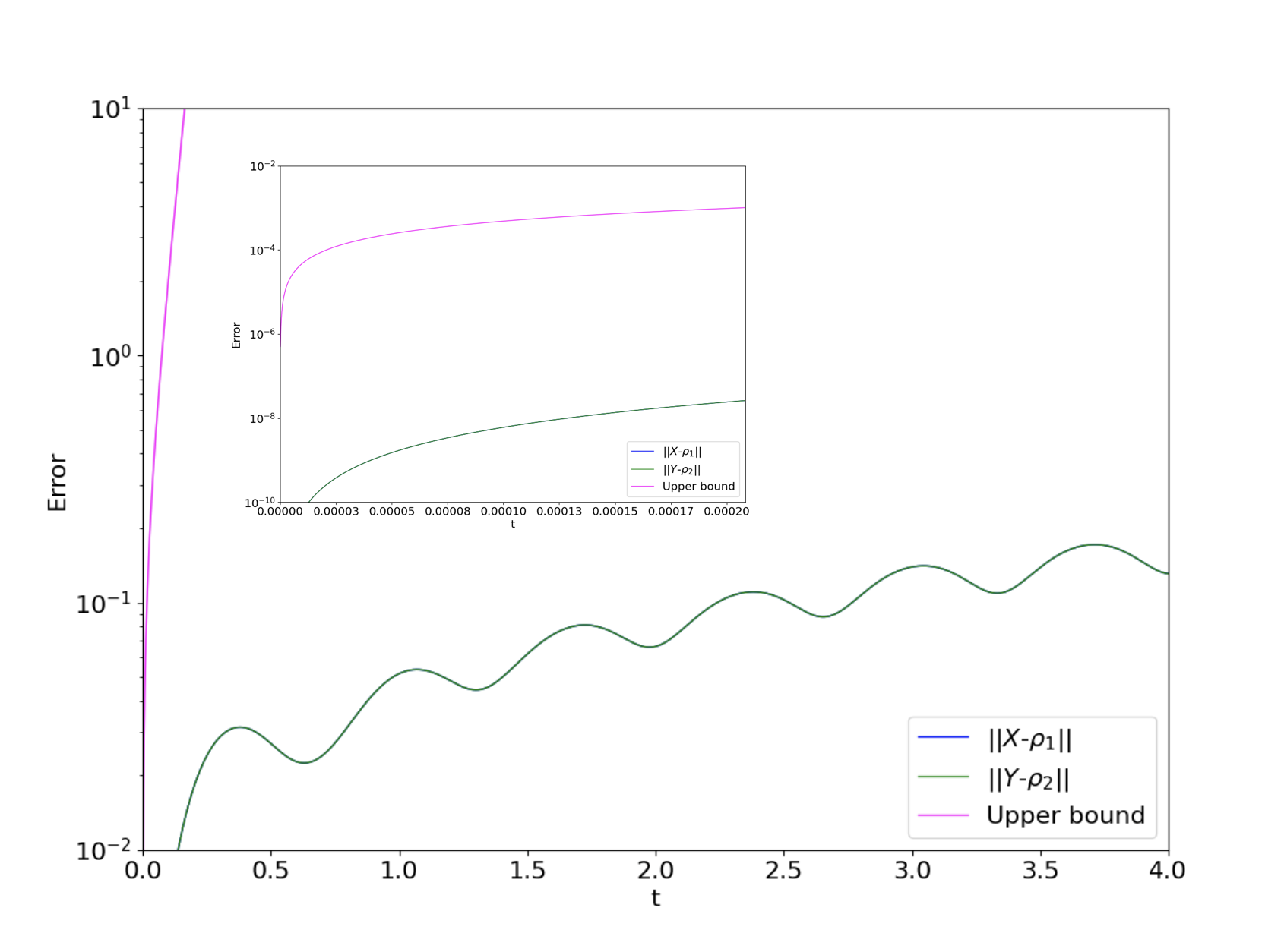
First consider the $\lambda=1$ simulation results shown in Figs. 1 and 2. Here qubit 1 is the central qubit and qubit 2 is an ancilla qubit. To read Fig. 1, note that the exact Bloch vector components ( $x_{1},\cdots,z_{2}$ ) are thicker lines, with qubit 1 solid and qubit 2 dashed. However the qubit 1 (solid) and qubit 2 (dashed) curves in this figure are identical due to permutation symmetry (so the dashed curves are not visible). Overall, mean field theory is very accurate for this 10-qubit system. The entanglement entropy (black curve) shows very little entanglement developing between the central qubit and remaining 9 ancilla. The mean field theory state errors are shown in Fig. 2. Upper bound is the bound (32-32). The inset magnifies the short-time regime corresponding to model error $\epsilon=10^{-3}$ . This is the set of times where the bound is below $\epsilon$ , the regime where the CSM reliably simulates nonlinear quantum mechanics to error $\epsilon$ .

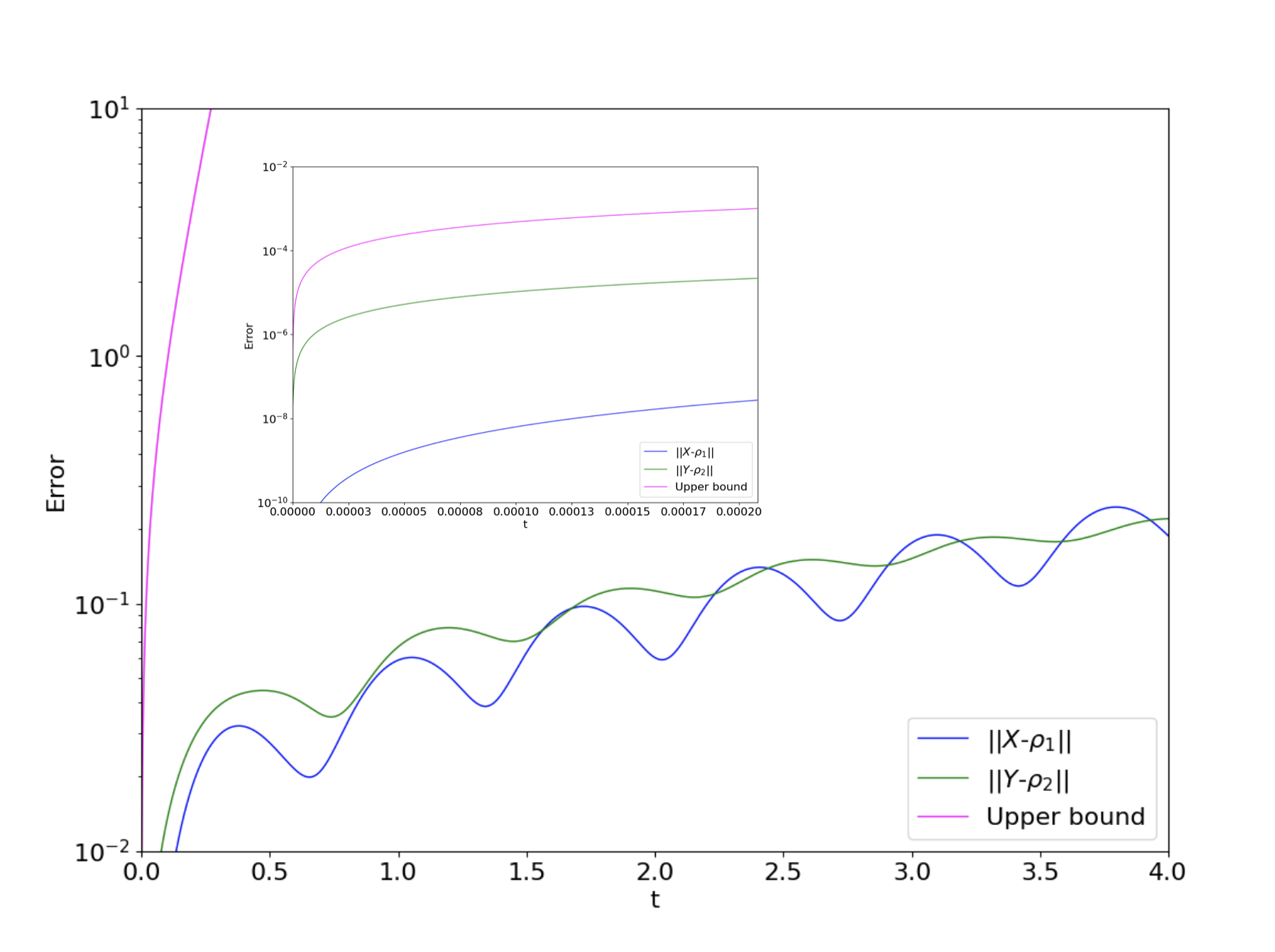
Figures 3 and 4 repeat this analysis for the $\lambda=0$ CSM. The main difference is that now the central qubit and ancilla have different dynamics. Also, the ancilla errors are usually larger than the central qubit state errors. This is a finite-size effect resulting from the $O(1/n)$ term neglected in passing from (24) to (25), which imparts an error on the equation of motion for the ancilla qubit $Y$ , but not on the central qubit $X$ . This asymmetry is especially apparent in the short-time regime.

References

Mielnik (1980) B. Mielnik, “Mobility of nonlinear systems,” J. Math. Phys. 21, 44 (1980).
Abrams and Lloyd (1998) D. S. Abrams and S. Lloyd, “Nonlinear quantum mechanics implies polynomial-time solution for NP-Complete and $\#$ P problems,” Phys. Rev. Lett. 81, 3992 (1998).
Bechmann-Pasquinucci et al. (1998) H. Bechmann-Pasquinucci, B. Huttner, and N. Gisin, “Nonlinear quantum state transformation of spin-1/2,” Phys. Lett. A 242, 198 (1998).
(4) S. Aaronson, “NP-complete problems and physical reality,” arXiv: quant-ph/0502072.
Childs and Young (2016) A. M. Childs and J. Young, “Optimal state discrimination and unstructured search in nonlinear quantum mechanics,” Phys. Rev. A 93, 022314 (2016).
Geller (2023) M. R. Geller, “Fast quantum state discrimination with nonlinear PTP channels,” Adv. Quantum Technol. , 2200156 (2023), arXiv: 2111.05977.
Czachor (1998) M. Czachor, “Notes on nonlinear quantum algorithms,” Acta Phys. Slov. 48, 157 (1998).
(8) M. Czachor, “Local modification of the Abrams-Lloyd nonlinear algorithm,” quant-ph/9803019.
Bacon (2004) D. Bacon, “Quantum computational complexity in the presence of closed timelike curves,” Phys. Rev. A 70, 032309 (2004).
Brun et al. (2009) T. A. Brun, J. Harrington, and M. M. Wilde, “Localized closed timelike curves can perfectly distinguish quantum states,” Phys. Rev. Lett. 102, 210402 (2009).
Bennett et al. (2009) C. H. Bennett, D. Leung, G. Smith, and J. A. Smolin, “Can closed timelike curves or nonlinear quantum mechanics improve quantum state discrimination or help solve hard problems?” Phys. Rev. Lett. 103, 170502 (2009).
Kahou and Feder (2013) M. E. Kahou and D. L. Feder, “Quantum search with interacting Bose-Einstein condensates,” Phys. Rev. A 88, 032310 (2013).
Meyer and Wong (2013) D. A. Meyer and T. G. Wong, “Nonlinear quantum search using the Gross-Pitaevskii equation,” New J. Phys. 15, 063014 (2013).
Meyer and Wong (2014) D. A. Meyer and T. G. Wong, “Quantum search with general nonlinearities,” Phys. Rev. A 89, 012312 (2014).
(15) G. Di Molfetta and B. Herzog, “Searching via nonlinear quantum walk on the 2D-grid,” arXiv: 2009.07800.
Deffner (2022) S. Deffner, “Nonlinear speed-ups in ultracold quantum gases,” Europhys. Lett. 140, 48001 (2022).
Xu and Sanders (2022) J. Xu, S.and Schmiedmayer and B. C. Sanders, “Nonlinear quantum gates for a Bose-Einstein condensate,” Phys. Rev. Research 4, 023071 (2022).
Yukawa et al. (2013) M. Yukawa, K. Miyata, H. Yonezawa, P. Marek, R. Filip, and A. Furusawa, “Emulating quantum cubic nonlinearity,” Phys. Rev. A 88, 053816 (2013).
Lee et al. (2015) C.-W. Lee, P. Kurzyński, and H. Nha, “Quantum walk as a simulator of nonlinear dynamics: Nonlinear Dirac equation and solitons,” Phys. Rev. A 92, 052336 (2015).
Joseph (2020) I. Joseph, “Koopman–von Neumann approach to quantum simulation of nonlinear classical dynamics,” Phys. Rev. Research 2, 043102 (2020).
Gaitan (2020) F. Gaitan, “Finding flows of a Navier–Stokes fluid through quantum computing,” npj Quantum Information 6, 61 (2020).
Liu et al. (2021) J.-P. Liu, H. Kolden, H. K. Krovi, N. F. Loureiro, K. Trivisa, and A. M. Childs, “Efficient quantum algorithm for dissipative nonlinear differential equations,” PNAS 118, e2026805118 (2021).
(23) S. Lloyd, G. De Palma, C. Gokler, B. Kiani, Z.-W. Liu, M. Marvian, F. Tennie, and T. Palmer, “Quantum algorithm for nonlinear differential equations,” arXiv: 2011.06571.
Engel et al. (2021) A. Engel, G. Smith, and S. E. Parker, “Linear embedding of nonlinear dynamical systems and prospects for efficient quantum algorithms,” Phys. Plasmas 28, 062305 (2021).
(25) L. Budinski, “Quantum algorithm for the Navier-Stokes equations,” arXiv: 2103.03804.
(26) I. Y. Dodin and E. A. Startsev, “Quantum computation of nonlinear maps,” arXiv: 2105.07317.
Dodin and Startsev (2021) I. Y. Dodin and E. A. Startsev, “On applications of quantum computing to plasma simulations,” Phys. Plasmas 28, 092101 (2021).
(28) N. Guo, K. Mitarai, and K. Fujii, “Nonlinear transformation of complex amplitudes via quantum singular value transformation,” arXiv: 2107.10764.
Xue et al. (a) C. Xue, Y.-C. Wu, and G.-P. Guo, “Quantum Newton’s method for solving system of nonlinear algebraic equations,” (a), arXiv: 2109.08470.
Xue et al. (b) C. Xue, Y.-C. Wu, and G.-P. Guo, “Quantum homotopy perturbation method for nonlinear dissipative ordinary differential equations,” (b), arXiv: 2111.07486.
(31) A. Shukla and P. Vedula, “A hybrid classical-quantum algorithm for solution of nonlinear ordinary differential equations,” arXiv: 2112.00602.
Holmes et al. (2023) Z. Holmes, N. Coble, A. T. Sornborger, and Y. Subaşı, “Nonlinear transformations in quantum computation,” Phys. Rev. Research 5, 013105 (2023).
(33) Y. T. Lin, R. B. Lowrie, D. Aslangil, Y. Subaşı, and A. T. Sornborger, “Koopman von Neumann mechanics and the Koopman representation: A perspective on solving nonlinear dynamical systems with quantum computers,” arXiv: 2202.02188.
Spohn (1980) H. Spohn, “Kinetic equations from Hamiltonian dynamics: Markovian limits,” Rev. Mod. Phys. 53, 569 (1980).
Bardos et al. (2000) C. Bardos, F. Golse, and N. J. Mauser, “Weak coupling limit of the N-particle Schrodinger equation,” Methods and Applications of Analysis 7, 275 (2000).
(36) C. Gokler, “Mean field limit for many-particle interactions,” arXiv: 2006.05486.
Fröhlich et al. (2007) J. Fröhlich, S. Graffi, and S. Schwarz, “Mean-field and classical limit of many-body Schrödinger dynamics for bosons,” Comm. Math. Phys. 271, 681 (2007).
Erdős et al. (2007) L. Erdős, B. Schlein, and H.-T. Yau, “Rigorous derivation of the Gross-Pitaevskii equation,” Phys. Rev. Lett. 98, 040404 (2007).
Rodnianski and Schlein (2009) I. Rodnianski and B. Schlein, “Quantum fluctuations and rate of convergence towards mean field dynamics,” Comm. Math. Phys. 291, 31 (2009).
Erdős and Schlein (2009) L. Erdős and B. Schlein, “Quantum dynamics with mean field interactions: A new approach,” J. Stat. Phys. 134, 859 (2009).
Knowles and Pickl (2010) A. Knowles and P. Pickl, “Mean-field dynamics: Singular potentials and rate of convergence,” Commun. Math. Phys. 298, 101 (2010).
Chen et al. (2011) L. Chen, J. O. Lee, and B. Schlein, “Rate of convergence towards Hartree dynamics,” J. Stat. Phys. 144, 872 (2011).
(43) Z. Ammari, M. Falconi, and B. Pawilowski, “On the rate of convergence for the mean field approximation of many-body quantum dynamics,” arXiv: 1411.6284v1.
Pickl (2015) P. Pickl, “Derivation of the time dependent Gross–Pitaevskii equation with external fields,” Reviews in Mathematical Physics 27, 1550003 (2015).
Benedikter et al. (2016) N. Benedikter, M. Porta, and B. Schlein, Effective Evolution Equations from Quantum Dynamics (Springer, Berlin, 2016).
Fröhlich et al. (2019) J. Fröhlich, A. Knowles, B. Schlein, and V. Sohinger, “A microscopic derivation of time-dependent correlation functions of the 1D cubic nonlinear Schrödinger equation,” Advances in Mathematics 353, 67 (2019).
Brennecke and Schlein (2019) C. Brennecke and B. Schlein, “Gross-Pitaevskii dynamics for Bose-Einstein condensates,” Analysis and PDE 12, 1513 (2019).
(48) A. Meill and D. A. Meyer, “Mean field approximation for identical bosons on the complete graph,” arXiv: 1910.14521.
Ellis (1985) R. S. Ellis, Entropy, Large Deviations, and Statistical Mechanics, GrundlehrenderMathematischen Wissenschaften, Vol. 271 (Springer, Berlin, 1985).
Gaudin (1976) M. Gaudin, “Diagonalisation d’une classe d’Hamiltoniens de spin,” J. Phys. France 37, 1087 (1976).
Yuzbashyan et al. (2005) E. A. Yuzbashyan, B. L. Altshuler, V. B. Kuznetsov, and V. Z. Enolskii, “Solution for the dynamics of the BCS and central spin problems,” J. Phys. A 38, 7831 (2005).
Bortz et al. (2010) M. Bortz, S. Eggert, C. Schneider, R. Stubner, and J. Stolze, “Dynamics and decoherence in the central spin model using exact methods,” Phys. Rev. B 82, 161308 (2010).
He et al. (2019) W.-B. He, S. Chesi, H.-Q Lin, and X.-W. Guan, “Exact quantum dynamics of XXZ central spin problems,” Phys. Rev. B 99, 174308 (2019).
He et al. (2022) W.-B. He, S. Chesi, H.-Q Lin, and X.-W. Guan, “Quantum dynamics of Gaudin magnets,” Commun. Theor. Phys. 74, 095102 (2022).
(55) N. V. Prokofev and P. C. E. Stamp, “Decoherence in the quantum dynamics of a central spin coupled to a spin environment,” arXiv: cond-mat/9511011.
Bortz and Stolze (2007) M. Bortz and J. Stolze, “Spin and entanglement dynamics in the central-spin model with homogeneous couplings,” J. Stat. Mech. (2007), 10.1088/1742-5468/2007/06/P06018.
(57) J. Ruh, R. Finsterhoelzl, and G. Burkard, “Digital quantum simulation of the BCS model with a central- spin-like quantum processor,” arXiv: 2209.09225.
Kessler et al. (2012) E. M. Kessler, G. Giedke, A. Imamoglu, S. F. Yelin, M. D. Lukin, and J. I. Cirac, “Dissipative phase transition in a central spin system,” Phys. Rev. A 86, 012116 (2012).
Mukhopadhyay et al. (2017) C. Mukhopadhyay, S. Bhattacharya, A. Misra, and A. K. Pati, “Dynamics and thermodynamics of a central spin immersed in a spin bath,” Phys. Rev. A 96, 052125 (2017).
Nachtergaele et al. (2006) B. Nachtergaele, Y. Ogata, and R. Sims, “Propagation of correlations in quantum lattice systems,” J. Stat. Phys. 124, 1 (2006).
Khaneja and Glaser (2001) N. Khaneja and S. J. Glaser, “Cartan decomposition of SU( $2^{n}$ ) and control of spin systems,” Chem. Phys. 267, 11 (2001).
Fesciyan (1973) S. Fesciyan, “The BBGKY hierarchy in quantum statistical mechanics,” Comm. Math. Phys. 30, 11 (1973).
Fernengel and Drossel (2020) B. Fernengel and B. Drossel, “Bifurcations and chaos in nonlinear Lindblad equations,” J. Phys. A: Math. Theor. 53, 385701 (2020).
(64) W. Kłobus, P. Kurzyński, M. Kuś, W. Laskowski, R. Przybycień, and K. Życzkowski, “Transition from order to chaos in reduced quantum dynamics,” arXiv: 2111.13477.
Lieb and Robinson (1972) E. H. Lieb and D. W. Robinson, “The finite group velocity of quantum spin systems,” Comm. Math. Phys. 28, 251 (1972).
Weinberg (1989a) S. Weinberg, “Testing quantum mechanics,” Ann. Phys. 194, 336 (1989a).
Weinberg (1989b) S. Weinberg, “Precision tests of quantum mechanics,” Phys. Rev. Lett. 62, 485 (1989b).
Bollinger et al. (1989) J. J. Bollinger, D. J. Heinzen, W. M. Itano, S. L. Gilbert, and D. J. Wineland, “Test of the linearity of quantum mechanics by rf spectroscopy of the ⁹Be⁺ ground state,” Phys. Rev. Lett. 63, 1031 (1989).
Chupp and Hoare (1990) T. E. Chupp and R. J. Hoare, “Coherence in freely precessing ${}^{21}\mathrm{Ne}$ and a test of linearity of quantum mechanics,” Phys. Rev. Lett. 64, 2261 (1990).
Walsworth et al. (1990) R. L. Walsworth, I. F. Silvera, E. M. Mattison, and R. F. C. Vessot, “Test of the linearity of quantum mechanics in an atomic system with a hydrogen maser,” Phys. Rev. Lett. 64, 2599 (1990).
Majumder et al. (1990) P. K. Majumder, B. J. Venema, S. K. Lamoreaux, B. R. Heckel, and E. N. Fortson, “Test of the linearity of quantum mechanics in optically pumped ²⁰¹Hg,” Phys. Rev. Lett. 65, 2931 (1990).
Forstner et al. (2020) S. Forstner, M. Zych, S. Basiri-Esfahani, K. E. Khosla, and W. P. Bowen, “Nanomechanical test of quantum linearity,” Optica 7, 1427 (2020).
Gisin (1990) N. Gisin, “Weinberg’s nonlinear quantum mechanics and supraluminal communication,” Phys. Lett. A 143, 1 (1990).
Polchinski (1991) J. Polchinski, “Weinberg’s nonlinear quantum mechanics and the Einstein-Podolsky-Rosen paradox,” Phys. Rev. Lett. 66, 397 (1991).
Gisin and Rigo (1995) N. Gisin and M Rigo, “Relevant and irrelevant nonlinear Schrodinger equations,” J. Phys. A 28, 7375 (1995).
Czachor and Doebner (2002) M. Czachor and H.-D. Doebner, “Correlation experiments in nonlinear quantum mechanics,” Phys. Lett. A 301, 139 (2002).
Kent (2005) A. Kent, “Nonlinearity without superluminality,” Phys. Rev. A 72, 012108 (2005).
Doebner et al. (1999) H.-D. Doebner, G. A. Goldin, and P Nattermann, “Gauge transformations in quantum mechanics and the unification of nonlinear Schrödinger equations,” J. Math. Phys. 40, 49 (1999).
Kibble (1978) T. W. B. Kibble, “Relativistic models of nonlinear quantum mechanics,” Comm. Math. Phys. 64, 73 (1978).
(80) G. Svetlichny, “Quantum evolution and space-time structure,” quant-ph/9512004.
(81) S. Lloyd, “The universe as quantum computer,” arXiv: 1312.4455.
(82) W. D. Wick, “On nonlinear quantum mechanics, space-time wavefunctions, and compatibility with general relativity,” arXiv: 2008.08663.
Kaplan and Rajendran (2022) D. E. Kaplan and S. Rajendran, “Causal framework for nonlinear quantum mechanics,” Phys. Rev. D 105, 055002 (2022).

	$\displaystyle\frac{\big\|{\rm tr}\big(A_{1}(X-\rho_{1})\big)\big\|}{\\|A_{1}\\|_{\infty}}\leq 6J_{0}\,\int_{0}^{t}\!d\tau\bigg\{\\|X-\rho_{1}\\|_{1}+\\|Y-\rho_{2}\\|_{1}+4\,\frac{e^{12(1\!+\!\|\lambda\|)J_{0}\tau}-1}{n-1}\bigg\},$		(71)
	$\displaystyle\frac{\big\|{\rm tr}\big(B_{2}(Y-\rho_{2})\big)\big\|}{\\|B_{2}\\|_{\infty}}\leq\frac{6J_{0}}{n-1}\int_{0}^{t}\!d\tau\bigg\{\\|X-\rho_{1}\\|_{1}+\\|Y-\rho_{2}\\|_{1}+4\,\frac{e^{12(1\!+\!\|\lambda\|)J_{0}\tau}-1}{n-1}$
	$\displaystyle+\|\lambda\|(n-2)\bigg(\!2\,\\|Y-\rho_{2}\\|_{1}+4\,\frac{e^{12(1\!+\!\|\lambda\|)J_{0}\tau}-1}{n-1}\bigg)\bigg\}.$		(72)

	$\displaystyle\sup_{A\neq 0}\frac{\big\|{\rm tr}\big(A_{1}(X-\rho_{1})\big)\big\|}{\\|A_{1}\\|_{\infty}}\leq 6J_{0}\,\int_{0}^{t}\!d\tau\bigg\{\\|X-\rho_{1}\\|_{1}+\\|Y-\rho_{2}\\|_{1}+4\,\frac{e^{12(1\!+\!\|\lambda\|)J_{0}\tau}-1}{n-1}\bigg\},$		(73)
	$\displaystyle\sup_{B\neq 0}\frac{\big\|{\rm tr}\big(B_{2}(Y-\rho_{2})\big)\big\|}{\\|B_{2}\\|_{\infty}}\leq\frac{6J_{0}}{n-1}\int_{0}^{t}\!d\tau\bigg\{\\|X-\rho_{1}\\|_{1}+\\|Y-\rho_{2}\\|_{1}+4\,\frac{e^{12(1\!+\!\|\lambda\|)J_{0}\tau}-1}{n-1}$
	$\displaystyle+\|\lambda\|(n-2)\bigg(\!2\,\\|Y-\rho_{2}\\|_{1}+4\,\frac{e^{12(1\!+\!\|\lambda\|)J_{0}\tau}-1}{n-1}\bigg)\bigg\}.$		(74)

	$\displaystyle\\|X-\rho_{1}\\|_{1}\leq 6J_{0}\,\int_{0}^{t}\!d\tau\bigg\{\\|X-\rho_{1}\\|_{1}+\\|Y-\rho_{2}\\|_{1}+4\,\frac{e^{12(1\!+\!\|\lambda\|)J_{0}\tau}-1}{n-1}\bigg\},$		(75)
	$\displaystyle\\|Y-\rho_{2}\\|_{1}\leq\frac{6J_{0}}{n-1}\int_{0}^{t}\!d\tau\bigg\{\\|X-\rho_{1}\\|_{1}+\\|Y-\rho_{2}\\|_{1}+4\,\frac{e^{12(1\!+\!\|\lambda\|)J_{0}\tau}-1}{n-1}$
	$\displaystyle+\|\lambda\|(n-2)\bigg(\!2\,\\|Y-\rho_{2}\\|_{1}+4\,\frac{e^{12(1\!+\!\|\lambda\|)J_{0}\tau}-1}{n-1}\bigg)\bigg\}.$		(76)

The universe as a nonlinear quantum simulation: Large nn limit of the central spin model