DProST: Dynamic Projective Spatial Transformer Network for 6D Pose Estimation

The overall process of DProST is shown in Fig. 2. We follow the zoom-in setting used in [22, 19, 21]. Hence, the off-the-shelf detector is first used to find the bounding box area of the object $I_{B}$ from the overall image $I$, where the bounding box is $B=(x,y,w,h)$.

Then, the space-carving-based reconstruction stage generates a reference feature $\mathcal{F}$ in the object space’s unit sphere based on the reference set $\mathcal{R}=\left\{\left(I^{\mathcal{R}}_{k},M^{\mathcal{R}}_{k},\bar{T}^{\mathcal{R}}_{k},K^{\mathcal{R}}_{k}\right)|k\in\left[1,N^{\mathcal{R}}\right]\right\}$ consists of $N^{\mathcal{R}}$ tuples of images $I^{\mathcal{R}}_{k}$ and masks $M^{\mathcal{R}}_{k}$ with known poses $\bar{T}^{\mathcal{R}}_{k}$ and intrinsic matrices $K^{\mathcal{R}}_{k}$ sampled from training set, which can be written as

We will discuss the details about the reconstruction stage in Section 3.3.

Subsequently, we iteratively refine the initial pose $T_{0}$ based on the $\mathcal{F}$ and $I_{B}$. Each pose refinement iteration $i$ consists of three submodules. First, based on a bounding box $B$, object pose $T_{i}=\{R_{i},t_{i}\}$, and intrinsic camera parameter $K$, grid generator extracts a localized RoI grid as

on the rays from the camera to the image plane in object space. Grid generator is composed of four sub-steps, grid forming, grid cropping, grid pushing, and grid transformation, and we will discuss the details of each step in Section 3.2.

The projector renders object appearance $X_{i}$ of each iteration by sampling features from $\mathcal{F}$ based on $\mathcal{G}_{i}^{obj}$ that can be written as

The projection stage plays a similar role to mesh rendering in [21, 19]. It can also be replaced with mesh rendering methods when the reference pose is not diverse enough to carve the object shape in the reconstruction stage.

Finally, to refine the pose, the pose estimator network of the $i$-th iteration with parameter $\theta_{i}$ predicts the relative pose $\Delta T_{i}$ between $X_{i}$ and $I_{B}$ as

The details of the projection stage and pose estimator are discussed in Section 3.4. Finally, we will address the overall objective function in Section 3.5.

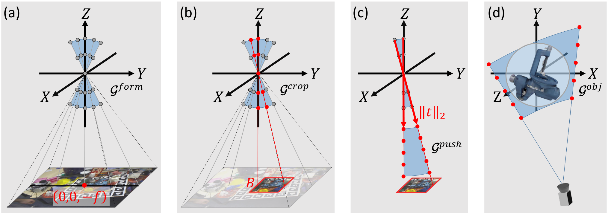
Grid generator in DProST converts the given intrinsic matrix ($K$), object pose ($T$), and bounding box ($B$) to the RoI grid in object space ($\mathcal{G}^{obj}$). Two key ideas are used for RoI grid localization. First, as the object’s projection is included in the bounding box, the object in camera space is in the ray’s direction, which passes through the bounding box area. Second, the distance to the object is the size of the translation vector in object pose.

In this section, we present a non-learning-required and a simple space-carving-based reference feature generation method. To generate the reference feature $\mathcal{F}$ in the unit sphere of the object space, we use pose-known reference images $\{X^{k}|k\in[1,N^{\mathcal{R}}]\}$ and corresponding masks $\{M^{k}|k\in[1,N^{\mathcal{R}}]\}$ sampled from the training set. The reference quality is improved when the various views and fine details are included. Hence, we set the first reference image as the sample with the largest object mask in the training set. Then, based on the geodesic distance of the rotation matrix, we use the farthest point sampling (FPS) algorithm in [31] to select the other reference images. We generate a 3D canvas as a normalized voxel grid $\mathcal{A}\in\mathbb{R}^{S\times S\times S\times 3}$, which is divided uniformly into $S^{3}$ voxels, and each contains the coordinates of itself. Then, for each reference mask and image, $\mathcal{A}$ is projected with the given $K$ and the pose of the $k$-th reference $\bar{T}^{k}$ to find the region where the canvas grid is projected. Hence, we assign the projected canvas location in $A^{k}$ as

where $\pi(p,K)$ represents the projection of the point $p$ with the intrinsic matrix $K$ in the pinhole camera model. Then, using $A^{k}$ as a grid, we apply the grid sampling method proposed in [17] to generate a 3D RGB feature $\mathcal{X}^{k}\in\mathbb{R}^{S\times S\times S\times 3}$ from $X^{k}$ and a 3D mask feature $\mathcal{M}^{k}\in\mathbb{R}^{S\times S\times S\times 1}$ from $M^{k}$ as follows:

where $\left(a^{k}\right)_{x}$ and $\left(a^{k}\right)_{y}$ are $\left(x,y\right)$ coordinates in $A^{k}$. Note that we use nearest-neighbor interpolation to extract values from non-integer locations. Then, we average the $\mathcal{X}^{k\in[1,N^{\mathcal{R}}]}$’s to obtain the integrated 3D RGB feature $\mathcal{X}$, and multiply $\mathcal{M}^{k\in[1,N^{\mathcal{R}}]}$’s to get the shape-carved 3D mask feature $\mathcal{M}$. Finally, the 3D features of the object are calculated as

where $\mathcal{F}\in\mathbb{R}^{S\times S\times S\times 3}$ is an RGB 3D feature with a carved shape with the object information in voxel fashion, and $\odot$ is an element-wise multiplication. The concept of carving process is visualized in Fig. 4.

With the $\mathcal{G}^{obj}$ obtained from grid generator and the reference feature $\mathcal{F}$, we apply the grid sampling [9], which can be written as

where $\mathcal{F}^{interp}\in\mathbb{R}^{h\times w\times N_{z}\times 3}$ is the sampled feature of the object and $interp$ is the trilinear interpolation-based grid sampling function.

Then, to compare the estimated pose and $I_{B}$, we project $\mathcal{F}^{interp}$ into a 2D feature $F\in\mathbb{R}^{h\times w\times 3}$ by choosing the closest valid point to the camera on each ray as

where $\delta\left(l,m\right)=\{n|\mathcal{F}^{interp}\left(l,m,n\right)\neq 0\}$.

For each iteration $i$, we use a ResNet34 [11] based pose estimator to refine the pose $T_{i-1}$ to $T_{i}$ to match the projected reference $F_{i-1}$ to the detected object image $I_{B}$. The last layer of ResNet34 is replaced with a fully connected layer that outputs nine values, each of which is image space translation, scale factor, and two axis-based relative rotation representation as in [19]. See the supplementary materials for more details about the pose estimator’s output format.

Instead of PM loss based on the mesh vertices of the object, we propose GM loss for mesh-less training. For each iteration $i$, we use the Euclidean distance of the object space grid as the GM loss, which can be written as

where $|\mathcal{G}^{obj}_{i}|$ is the number of points in the grid, $\mathcal{\bar{G}}^{obj}$ is a grid from the ground-truth pose $\bar{T}$, and $\mathcal{G}^{obj}_{i}$ is the predicted object space grid. Note that, as the DProST module is based on fully differentiable operations, the $i$-th GM loss is used as an objective function for the $i$-th pose estimator, as shown in Fig. 2.

Additionally, to help the pose estimator determine the distance from the camera to the object in the grid pushing step, we use an auxiliary loss called GD loss as

which is the absolute difference between the predicted distance and ground-truth distance in the grid pushing step.

Finally, the overall loss $\mathcal{L}_{i}$ for training our network on each iteration $i$ is the combination of the above two losses as

where $\lambda^{GD}$ is the balance factor. The $\mathcal{L}_{i}$ is applied to outputs of each iterations’ pose estimator.

The performance is tested on LINEMOD (LM) [12], LINEMOD-OCCLUSION (LMO) [1], and YCB-video (YCBV) dataset [42]. The LM consists of 13 objects with approximately 1.2K images per object. We follow the settings described in [2], which uses 15% of the data for training and the rest for testing. The LMO dataset is a subset of the LM dataset consisting of eight objects in more cluttered scenes. The YCBV dataset consists of 21 objects with between 10k and 20k real images per object. The YCBV dataset is very hard compared to the LM dataset because of the hard occluded samples. Also, the views in YCBV dataset are not as various as the LM dataset. We used the official pbr dataset from the BOP challenge [13] in training along with the real image training set. For the LM dataset, we also report the performance trained on the synthetic training dataset introduced from [21].

The $ADD(\textbf{-}S)$ score [12] is used to measure the performance, which is the most widely employed metric in the object pose estimation [42, 21, 37, 40, 37, 16]. In particular, we use the $ADD$ score for non-symmetric objects, which computes the pair-wise distance of vertices transformed by the predicted pose and ground-truth pose. And we use the $ADD\textbf{-}S$ score for symmetric objects, which measures the nearest distance of transformed vertices by predicted pose and ground-truth pose. The predicted pose is considered correct if the mean distance is less than the threshold ratio $thr$ of the object diameter in the $ADD(\textbf{-}S)^{thr}$ metric. The area-under-curve of the $ADD(\textbf{-}S)$ metric [42] is additionally used for the YCBV dataset.

We also compare the projection error $Proj2D$ [21], which measures the pixel-level discrepancy of the projected vertices in the image space.

Table 1 presents the results on the LM dataset. As shown in the table, our method shows state-of-the-art accuracy on the LM dataset even without mesh data. Compared to a point matching-based method [21], which uses mesh vertices, our method shows more accurate results for almost every object.

Also, the accuracy of the LMO dataset is described in Table 2, and our method shows state-of-the-art performance. Some qualitative results on the LMO dataset are shown in Fig. 5. The figure shows that even the low-quality texture reference from the simple space-carving is enough for most samples.

However, we confirm that the reference feature-based projection is vulnerable to some conditions. For example, when the overall training view is similar, such as a video-based training set, or when majority of the samples are occluded, the shape of the reference quality is degraded. Because the YCBV has these characteristics, our reconstruction module fails to generate a plausible shape of the reference feature of some objects as shown in Fig. 6(a), therefore we used the mesh-based renderer in pytorch3d instead of our projector in the YCBV dataset. As stated in Table 3, our model shows comparable performance to other state-of-the-art methods on the YCBV dataset. We also visualize some qualitative results of the YCBV dataset in Fig. 6(b). More qualitative results and comparisons with the other state-of-the-art methods are included in the supplementary material.

We conduct several ablation studies on the LM dataset. First, we test our method with the number of iterations as shown in Table 4 $left$. The result shows that the performance is improved in the second iteration but saturates in more iterations. We visualize an example of iterative refinement in Fig. 6(c).

We also visualize $\mathcal{G}^{obj}$s of the qualitative results in Fig. 6(b), (c). As shown in the figure, the difference of the grid area toward the camera and the opposite is caused by projective geometry. And since the ratio of two areas is inversely proportional to the object’s distance, the shape of the $\mathcal{G}^{obj}$ reflects the object distance information. Consequently, as the GM loss leverages the shape of the $\mathcal{G}^{obj}$ to learn the distance, training even without GD loss is successful, as shown in Table 4 $middle$. In other words, projective geometry helps our method to learn the distance to the object. We also confirm that $L^{GD}$ improves the performance, especially on the $ADD(\textbf{-}S)$ score, since it helps estimate more accurate distance of the grid in camera space. Additionally, the effect of GM loss compared to PM loss and image matching loss is reported in the supplementary material.

The performance about the number of points per ray ($N_{z}$) is in Table 4 $right$, and $N_{z}=64$ shows the best in both $ADD(\textbf{-}S)$ and $Proj2D$ score.

Table 5 $left$ shows the experiment on the source of projection and view sampling method in reference feature. As demonstrated, a simple space-carving-based reference feature can replace the mesh without significant performance degradation, and FPS outperforms the random sampling of reference.

Finally, we conduct an ablation study of the number of views ($N^{\mathcal{R}}$) for the reference image in Table 5 $right$. As shown in the table, eight reference images show the best performance. Note that because each voxel value of the reference feature is the average of the reference image, if there are too many references, the texture becomes blurry, and performance suffer. The quality of the reference feature depending on the number of views is demonstrated in the supplementary material.

The experiments is conducted on an AMD Ryzen 9 3900X 12-Core CPU with an NVIDIA Geforce RTX 2080Ti GPU. In addition to the 1.21 s for space carving and 15 ms in detection, our method takes 0.22 ms in grid generator, 2.06ms in the projector, and 3.86 ms in the pose estimator for each step. Note that, since our method focuses on the seen object scenario, the reference feature is created only once for each object in training phase and used repeatedly without additional generation. Because the grid from the grid generator is directly used as a sampling grid, our projector is faster than the mesh rendering function in pytorch3d, which takes 3.14 ms.

References

- [1] Brachmann, E., Krull, A., Michel, F., Gumhold, S., Shotton, J., Rother, C.: Learning 6d object pose estimation using 3d object coordinates. In: European conference on computer vision. pp. 536–551. Springer (2014)
- [2] Brachmann, E., Michel, F., Krull, A., Yang, M.Y., Gumhold, S., et al.: Uncertainty-driven 6d pose estimation of objects and scenes from a single rgb image. In: Proceedings of the IEEE conference on computer vision and pattern recognition. pp. 3364–3372 (2016)
- [3] Cai, Z., Vasconcelos, N.: Cascade r-cnn: Delving into high quality object detection. In: Proceedings of the IEEE conference on computer vision and pattern recognition. pp. 6154–6162 (2018)
- [4] Chen, X., Ma, H., Wan, J., Li, B., Xia, T.: Multi-view 3d object detection network for autonomous driving. In: Proceedings of the IEEE conference on Computer Vision and Pattern Recognition. pp. 1907–1915 (2017)
- [5] Chen, X., Dong, Z., Song, J., Geiger, A., Hilliges, O.: Category level object pose estimation via neural analysis-by-synthesis. In: European Conference on Computer Vision. pp. 139–156. Springer (2020)
- [6] Cheng, Y., Zhu, H., Sun, Y., Acar, C., Jing, W., Wu, Y., Li, L., Tan, C., Lim, J.H.: 6d pose estimation with correlation fusion. In: 2020 25th International Conference on Pattern Recognition (ICPR). pp. 2988–2994. IEEE (2021)
- [7] Deng, J., Dong, W., Socher, R., Li, L.J., Li, K., Fei-Fei, L.: Imagenet: A large-scale hierarchical image database. In: 2009 IEEE conference on computer vision and pattern recognition. pp. 248–255. Ieee (2009)
- [8] Di, Y., Manhardt, F., Wang, G., Ji, X., Navab, N., Tombari, F.: So-pose: Exploiting self-occlusion for direct 6d pose estimation. In: Proceedings of the IEEE/CVF International Conference on Computer Vision. pp. 12396–12405 (2021)
- [9] Gao, C., Liu, X., Gu, W., Killeen, B., Armand, M., Taylor, R., Unberath, M.: Generalizing spatial transformers to projective geometry with applications to 2d/3d registration. In: International Conference on Medical Image Computing and Computer-Assisted Intervention. pp. 329–339. Springer (2020)
- [10] He, K., Gkioxari, G., Dollár, P., Girshick, R.: Mask r-cnn. In: Proceedings of the IEEE international conference on computer vision. pp. 2961–2969 (2017)
- [11] He, K., Zhang, X., Ren, S., Sun, J.: Deep residual learning for image recognition. In: Proceedings of the IEEE conference on computer vision and pattern recognition. pp. 770–778 (2016)
- [12] Hinterstoisser, S., Lepetit, V., Ilic, S., Holzer, S., Bradski, G., Konolige, K., Navab, N.: Model based training, detection and pose estimation of texture-less 3d objects in heavily cluttered scenes. In: Asian conference on computer vision. pp. 548–562. Springer (2012)
- [13] Hodaň, T., Sundermeyer, M., Drost, B., Labbé, Y., Brachmann, E., Michel, F., Rother, C., Matas, J.: Bop challenge 2020 on 6d object localization. In: European Conference on Computer Vision. pp. 577–594. Springer (2020)
- [14] Hu, Y., Fua, P., Wang, W., Salzmann, M.: Single-stage 6d object pose estimation. In: Proceedings of the IEEE/CVF conference on computer vision and pattern recognition. pp. 2930–2939 (2020)
- [15] Hu, Y., Hugonot, J., Fua, P., Salzmann, M.: Segmentation-driven 6d object pose estimation. In: Proceedings of the IEEE/CVF Conference on Computer Vision and Pattern Recognition. pp. 3385–3394 (2019)
- [16] Iwase, S., Liu, X., Khirodkar, R., Yokota, R., Kitani, K.M.: Repose: Fast 6d object pose refinement via deep texture rendering. In: Proceedings of the IEEE/CVF International Conference on Computer Vision. pp. 3303–3312 (2021)
- [17] Jaderberg, M., Simonyan, K., Zisserman, A., et al.: Spatial transformer networks. Advances in neural information processing systems 28, 2017–2025 (2015)
- [18] Kingma, D.P., Ba, J.: Adam: A method for stochastic optimization. arXiv preprint arXiv:1412.6980 (2014)
- [19] Labbé, Y., Carpentier, J., Aubry, M., Sivic, J.: Cosypose: Consistent multi-view multi-object 6d pose estimation. In: European Conference on Computer Vision. pp. 574–591. Springer (2020)
- [20] Lepetit, V., Moreno-Noguer, F., Fua, P.: Epnp: An accurate o (n) solution to the pnp problem. International journal of computer vision 81(2), 155 (2009)
- [21] Li, Y., Wang, G., Ji, X., Xiang, Y., Fox, D.: Deepim: Deep iterative matching for 6d pose estimation. In: Proceedings of the European Conference on Computer Vision (ECCV). pp. 683–698 (2018)
- [22] Li, Z., Wang, G., Ji, X.: Cdpn: Coordinates-based disentangled pose network for real-time rgb-based 6-dof object pose estimation. In: Proceedings of the IEEE/CVF International Conference on Computer Vision. pp. 7678–7687 (2019)
- [23] Marchand, E., Uchiyama, H., Spindler, F.: Pose estimation for augmented reality: a hands-on survey. IEEE transactions on visualization and computer graphics 22(12), 2633–2651 (2015)
- [24] Mildenhall, B., Srinivasan, P.P., Tancik, M., Barron, J.T., Ramamoorthi, R., Ng, R.: Nerf: Representing scenes as neural radiance fields for view synthesis. In: European conference on computer vision. pp. 405–421. Springer (2020)
- [25] Nguyen-Phuoc, T., Li, C., Balaban, S., Yang, Y.L.: Rendernet: A deep convolutional network for differentiable rendering from 3d shapes. In: Advances in Neural Information Processing Systems 31 (2018)
- [26] Oberweger, M., Rad, M., Lepetit, V.: Making deep heatmaps robust to partial occlusions for 3d object pose estimation. In: Proceedings of the European Conference on Computer Vision (ECCV). pp. 119–134 (2018)
- [27] Park, K., Mousavian, A., Xiang, Y., Fox, D.: Latentfusion: End-to-end differentiable reconstruction and rendering for unseen object pose estimation. In: Proceedings of the IEEE/CVF conference on computer vision and pattern recognition. pp. 10710–10719 (2020)
- [28] Park, K., Patten, T., Vincze, M.: Pix2pose: Pixel-wise coordinate regression of objects for 6d pose estimation. In: Proceedings of the IEEE/CVF International Conference on Computer Vision. pp. 7668–7677 (2019)
- [29] Park, K., Patten, T., Vincze, M.: Neural object learning for 6d pose estimation using a few cluttered images. In: European Conference on Computer Vision. pp. 656–673. Springer (2020)
- [30] Paszke, A., Gross, S., Massa, F., Lerer, A., Bradbury, J., Chanan, G., Killeen, T., Lin, Z., Gimelshein, N., Antiga, L., et al.: Pytorch: An imperative style, high-performance deep learning library. Advances in neural information processing systems 32, 8026–8037 (2019)
- [31] Peng, S., Liu, Y., Huang, Q., Zhou, X., Bao, H.: Pvnet: Pixel-wise voting network for 6dof pose estimation. In: Proceedings of the IEEE/CVF Conference on Computer Vision and Pattern Recognition. pp. 4561–4570 (2019)
- [32] Rad, M., Lepetit, V.: Bb8: A scalable, accurate, robust to partial occlusion method for predicting the 3d poses of challenging objects without using depth. In: Proceedings of the IEEE International Conference on Computer Vision. pp. 3828–3836 (2017)
- [33] Ravi, N., Reizenstein, J., Novotny, D., Gordon, T., Lo, W.Y., Johnson, J., Gkioxari, G.: Accelerating 3d deep learning with pytorch3d. arXiv preprint arXiv:2007.08501 (2020)
- [34] Redmon, J., Farhadi, A.: Yolov3: An incremental improvement. arXiv preprint arXiv:1804.02767 (2018)
- [35] Ren, S., He, K., Girshick, R., Sun, J.: Faster r-cnn: Towards real-time object detection with region proposal networks. Advances in neural information processing systems 28, 91–99 (2015)
- [36] Sitzmann, V., Thies, J., Heide, F., Nießner, M., Wetzstein, G., Zollhofer, M.: Deepvoxels: Learning persistent 3d feature embeddings. In: Proceedings of the IEEE/CVF Conference on Computer Vision and Pattern Recognition. pp. 2437–2446 (2019)
- [37] Song, C., Song, J., Huang, Q.: Hybridpose: 6d object pose estimation under hybrid representations. In: Proceedings of the IEEE/CVF conference on computer vision and pattern recognition. pp. 431–440 (2020)
- [38] Tremblay, J., To, T., Sundaralingam, B., Xiang, Y., Fox, D., Birchfield, S.: Deep object pose estimation for semantic robotic grasping of household objects. In: Conference on Robot Learning. pp. 306–316. PMLR (2018)
- [39] Wang, C., Xu, D., Zhu, Y., Martín-Martín, R., Lu, C., Fei-Fei, L., Savarese, S.: Densefusion: 6d object pose estimation by iterative dense fusion. In: Proceedings of the IEEE/CVF conference on computer vision and pattern recognition. pp. 3343–3352 (2019)
- [40] Wang, G., Manhardt, F., Tombari, F., Ji, X.: Gdr-net: Geometry-guided direct regression network for monocular 6d object pose estimation. In: Proceedings of the IEEE/CVF Conference on Computer Vision and Pattern Recognition. pp. 16611–16621 (2021)
- [41] Wang, H., Sridhar, S., Huang, J., Valentin, J., Song, S., Guibas, L.J.: Normalized object coordinate space for category-level 6d object pose and size estimation. In: Proceedings of the IEEE/CVF Conference on Computer Vision and Pattern Recognition. pp. 2642–2651 (2019)
- [42] Xiang, Y., Schmidt, T., Narayanan, V., Fox, D.: Posecnn: A convolutional neural network for 6d object pose estimation in cluttered scenes. In: Proceedings of Robotics: Science and Systems. Pittsburgh, Pennsylvania (June 2018). https://doi.org/10.15607/RSS.2018.XIV.019
- [43] Xu, D., Anguelov, D., Jain, A.: Pointfusion: Deep sensor fusion for 3d bounding box estimation. In: Proceedings of the IEEE conference on computer vision and pattern recognition. pp. 244–253 (2018)
- [44] Yen-Chen, L., Florence, P., Barron, J.T., Rodriguez, A., Isola, P., Lin, T.Y.: inerf: Inverting neural radiance fields for pose estimation. In: 2021 IEEE/RSJ International Conference on Intelligent Robots and Systems (IROS). pp. 1323–1330. IEEE (2021)
- [45] Zakharov, S., Shugurov, I., Ilic, S.: Dpod: 6d pose object detector and refiner. In: Proceedings of the IEEE/CVF International Conference on Computer Vision. pp. 1941–1950 (2019)
- [46] Zhou, Y., Barnes, C., Lu, J., Yang, J., Li, H.: On the continuity of rotation representations in neural networks. In: Proceedings of the IEEE/CVF Conference on Computer Vision and Pattern Recognition. pp. 5745–5753 (2019)
- [47] Zhu, M., Derpanis, K.G., Yang, Y., Brahmbhatt, S., Zhang, M., Phillips, C., Lecce, M., Daniilidis, K.: Single image 3d object detection and pose estimation for grasping. In: 2014 IEEE International Conference on Robotics and Automation (ICRA). pp. 3936–3943. IEEE (2014)
Supplementary Material - DProST: Dynamic Projective Spatial Transformer Network for
6D Pose Estimation
Appendix 0.A Details of Pose Estimator
The disentangled representation is used for the pose estimator output as in [19]. For each iteration , our ResNet34 [11] based pose estimator predicts relative translation on image space, which can be written as follows: