Self-Supervised Dynamic Graph Representation Learning via Temporal Subgraph ContrastDOI: 10.1145/1122445.1122456Conference: Woodstock ’18: ACM Symposium on Neural Gaze Detection; June 03–05, 2018; Woodstock, NYWoodstock ’18: ACM Symposium on Neural Gaze Detection, June 03–05, 2018, Woodstock, NYPrice: 15.00ISBN: 978-1-4503-XXXX-X/18/06CCS: Theory of computation Dynamic graph algorithmsCCS: Computing methodologies Unsupervised learningCCS: Computing methodologies Learning latent representations
Abstract.
Self-supervised learning on graphs has recently drawn a lot of attention due to its independence from labels and its robustness in representation. Current studies on this topic mainly use static information such as graph structures but cannot well capture dynamic information such as timestamps of edges. Realistic graphs are often dynamic, which means the interaction between nodes occurs at a specific time. This paper proposes a self-supervised dynamic graph representation learning framework (DySubC), which defines a temporal subgraph contrastive learning task to simultaneously learn the structural and evolutional features of a dynamic graph. Specifically, a novel temporal subgraph sampling strategy is firstly proposed, which takes each node of the dynamic graph as the central node and uses both neighborhood structures and edge timestamps to sample the corresponding temporal subgraph. The subgraph representation function is then designed according to the influence of neighborhood nodes on the central node after encoding the nodes in each subgraph. Finally, the structural and temporal contrastive loss are defined to maximize the mutual information between node representation and temporal subgraph representation. Experiments on five real-world datasets demonstrate that (1) DySubC performs better than the related baselines including two graph contrastive learning models and four dynamic graph representation learning models in the downstream link prediction task, and (2) the use of temporal information can not only sample more effective subgraphs, but also learn better representation by temporal contrastive loss.
Keywords:
self-supervised learning, temporal subgraph contrast, dynamic graph representation learning1. Introduction
Graph-structured data, such as social networks (Chen et al. 2018), collaboration networks (Newman 2001) and chemical molecular graphs (Liao et al. 2019), are ubiquitous in the real world. They naturally represent entities and their relationships. Graph representation learning aims to transform nodes into low-dimensional dense embeddings that preserve attributive and structural features of the graph. The method of using graph neural networks (GNN) (Velickovic et al. 2018; Wu et al. 2019; Kipf and Welling 2017; Qu et al. 2019) has recently drawn considerable attention and achieved excellent performance. However, the supervised or semi-supervised GNNs heavily rely on labels with high acquisition cost, which could lead to poor generalization and weak robustness under label-related adversarial attacks (Liu et al. 2021).
Self-supervised learning can effectively alleviate the above problems. By designing appropriate training tasks on the graph, the self-supervised model can learn a more generalized graph representation in the absence of labels. Most of the existing methods focus on learning representations from the structural perspective by contrasting graph elements of different scales, such as node and local subgraph contrasting (Jiao et al. 2020), and node and global graph contrasting (Velickovic et al. 2019; Hassani and Ahmadi 2020).
However, neither graph sampling nor graph contrastive learning in these methods take the graph dynamics (especially the temporal information of edge generation) into account. As a result, the learned node representation cannot reflect the graph evolution. Take the social network in Figure 1 as an example, where the edge represents the friend relationship of two person nodes. Each edge is marked with a timestamp (), indicating the moment when they became friends. The central node Mary used to be an engineer, and most of her neighbor nodes were engineers before . Recently, Mary changed her career to become a teacher and started to have teacher neighbor nodes (e.g., she will friend a teacher at time ). The static graph representation learning model samples subgraphs and encodes the nodes only based on structures, so it could predict that Mary will friend an engineer instead of a teacher at time . By using temporal information, the dynamic subgraph sampling and node representation method can capture Mary’s relationship evolution, which may give a more accurate prediction.

Nodes are usually more closely related to their regional neighbors (Jiao et al. 2020). So intuitionally, frequent changes of neighbors will reflect potential changes of the central node and the latest neighbors that interacted with the central node are more valuable in node representation. This paper proposes a novel self-supervised dynamic graph representation learning method (DySubC), which learns node representation by sampling and contrasting with temporal subgraphs. To be specific, a temporal subgraph sampling strategy is firstly proposed, which takes each node as the central node to sample the corresponding temporal subgraph. The subgraphs are sampled by considering not only the local structure but also the temporal information of neighborhood interactions. Then, a certain GNN encoder is used to learn node representation for each temporal subgraph, thus output the representation of the central node and the summary of the temporal subgraph calculated by a time-aware readout function defined in this paper. Finally, the central node is paired with (a) its corresponding time-weighted subgraph as a positive sample, (b) any other temporal subgraph in a shuttled sampling set as a structural negative sample and (c) its corresponding unweighted subgraph as a temporal negative sample to train the whole model by maximizing the mutual information of the central node and its temporal subgraph.
In summary, the main contributions of the DySubC framework include:
- •
This paper studies the problem of dynamic graph contrast learning for the first time and better captures the structural evolution characteristics of graphs by introducing temporal information.
- •
A temporal subgraph sampling method is proposed, which simultaneously uses the structural and temporal information of neighborhoods.
- •
A new readout function is defined to get the summary of a temporal subgraph, which takes the influence of the neighborhood nodes on the central node into account.
- •
A temporal subgraph contrast loss is defined including structure contrast loss and time contrast loss.
- •
Extensive experiments verify the superiority of DySubC in link prediction compared to the related continuous time graph representation learning models and graph contrastive learning models. The ablation study further proves the effectiveness of each time-enhanced module.
The rest of this paper includes the following sections. In Section 2, the related work on dynamic graph representation learning and self-supervised graph learning is briefly reviewed. Section 3 introduces the proposed DySubC framework in detail. The experimental results are shown and analyzed in Section 4. Section 5 concludes the paper.
2. RELATED WORK
2.1. Dynamic Graph Representation Learning
Graph neural networks (GNNs) (Velickovic et al. 2018; Wu et al. 2019; Kipf and Welling 2017; Qu et al. 2019) have achieved the competitive performance in static graph representation learning (Perozzi et al. 2014; Grover and Leskovec 2016; Tang et al. 2015; Wang et al. 2016). Recently, the dynamic graph representation learning has drawn more and more attentions due to its ability to incorporate temporal information into representations. There are two different types of dynamic graphs, i.e., discrete time graphs and continuous time graphs. Accordingly, dynamic graph representation learning is also roughly divided into two categories.
Discrete time graph refers to a dynamic graph formalized as a series of multiple graph snapshots with the same time interval between them. This type of methods generally conduct representation learning on each snapshot first and then learns the evolution features of the graph structure over time through a sequence learning model (e.g., RNN (Zaremba et al. 2014), self-attention (Vaswani et al. 2017), etc.). Representative methods include DynGEM (Goyal et al. 2018), DynamicTriad (Zhou et al. 2018), EvolveGCN (Pareja et al. 2020), DySAT (Sankar et al. 2020) and so on. These methods focus more on capturing the global evolution features rather than the features of local continuous changes.
The continuous time graph is another formalization of dynamic graph where edges are marked with continuous timestamps. CTDNE (Nguyen et al. 2018) proposes a temporal random walk method and then uses skip-gram to obtain node representation. HTNE (Zuo et al. 2018) introduces the Hawkes process theory into the dynamic graph model and learns node representation based on the fact that the influence of neighbors on the central node will change over time. DyRep (Trivedi et al. 2019) captures the interleaved dynamics of communication processes and correlation processes, thereby updating node representation. TGN (Rossi et al. 2020) combines the memory module and graph-based operators to update node representations and improves the computational efficiency. The method proposed in this paper also falls into the category of continuous time graph representation learning, which mainly uses the changes of regional neighbors to learn node representations.
2.2. Self-supervised Graph Learning
Self-supervised learning uses pretext tasks to train the model with constructed supervised information from large-scale unsupervised data. It not only alleviates the problem of high cost of acquiring data labels, but also learns effective features. It has been successfully used in computer vision (Jing and Tian 2021) and natural language processing (Liu et al. 2020). For graph representation learning, DGI (Velickovic et al. 2019) is the first graph self-supervised learning method that uses the pretext task of maximizing mutual information between node representations and global graph representations. After that, a series of graph contrastive learning models emerged. Sankararaman et al. (Hassani and Ahmadi 2020) propose a multi-view graph contrastive learning model MVGRL, which treats the original graph structure and graph diffusion as two different views to maximize mutual information between nodes and cross-view representations of large-scale graphs. The graph contrastive learning in GMI (Peng et al. 2020) is achieved by maximizing the mutual information between the representation of each node and the original features of its one-hop neighbors. Sub-Con (Jiao et al. 2020) maximizes the mutual information between node representations and subgraph representations, which can be used for large-scale graphs.
In addition to the above methods, (Qiu et al. 2020; Zhu et al. 2020; Zhu et al. 2021) introduce the contrastive learning method (Chen et al. 2020) in machine vision into graph representation learning, which adopts different strategies for positive and negative sample construction and different loss functions.
However, the existing graph self-supervised methods do not take into consideration the fact that graphs in real world are often dynamic. The temporal information is not well used not only in the pretext task but also in the definition of the objective function. The work of this paper attempts to bridge this gap.
3. THE PROPOSED METHOD
3.1. Preliminaries
Before detailing the model, a formal definition of dynamic graph is given. Considering that the interaction between nodes occurs at a specific time and the graph is constantly changing over time, this paper models the dynamic graph as a continuous time graph.
Definition 1 (Dynamic Graphs). Given a graph , is a set of vertices, is a set of edges with timestamp and denotes the matrix of node attributes. represents the interaction between node and at time . Note that when the nodes are not attributed, one-hot encoding is often used to initialize .
Problem 1 (Continuous-time dynamic graph representation learning). For a dynamic graph , the task is to learn the mapping function to embed the node in a -dimensional vector space. The node representation is supposed to contain both structural and temporal information and suitable for downstream machine learning tasks such as link prediction.
3.2. Overview
The proposed DySubC (Dynamic graph representation learning via temporal Subgraph Contrast) framework uses graph contrastive learning that captures the structural and temporal features from continuous-time graphs during the training phase without additional supervision. An overview of the DySubC framework is shown in Figure 2, which mainly includes three time-enhanced modules.
- •
Temporal subgraph sampling. Firstly, a temporal subgraph for each node in the original graph is sampled using both structural and temporal information, generating a time-weighted subgraph and an unweighted counterpart .
- •
Node and subgraph representation. Secondly, and are encoded through GNN and then the summary of each subgraph is represented by a readout function, respectively. For each node , we have its representation , a time-weighted subgraph representation and an unweighted subgraph representation .
- •
Temporal contrastive learning. Finally, a positive sample , a temporal negative sample and a structural negative sample are constructed for each central node represented by . The model is trained by maximizing the mutual information of the central node representation and the time-weighted subgraph representation.
Note that the temporal subgraph sampling can be completed independently before the start of training. Thus, it does not take up the running time of the model.

3.3. Temporal Subgraph Sampling
The temporal subgraph sampling module is first proposed for each node to generate training samples for self-supervised learning.
By considering both the structure of neighbors and the timestamp of edge interactions, the temporal subgraph sampler (see Algorithm 1) can sample a temporal subgraph with a fixed number of nodes for each central node . The specific steps are as follows.
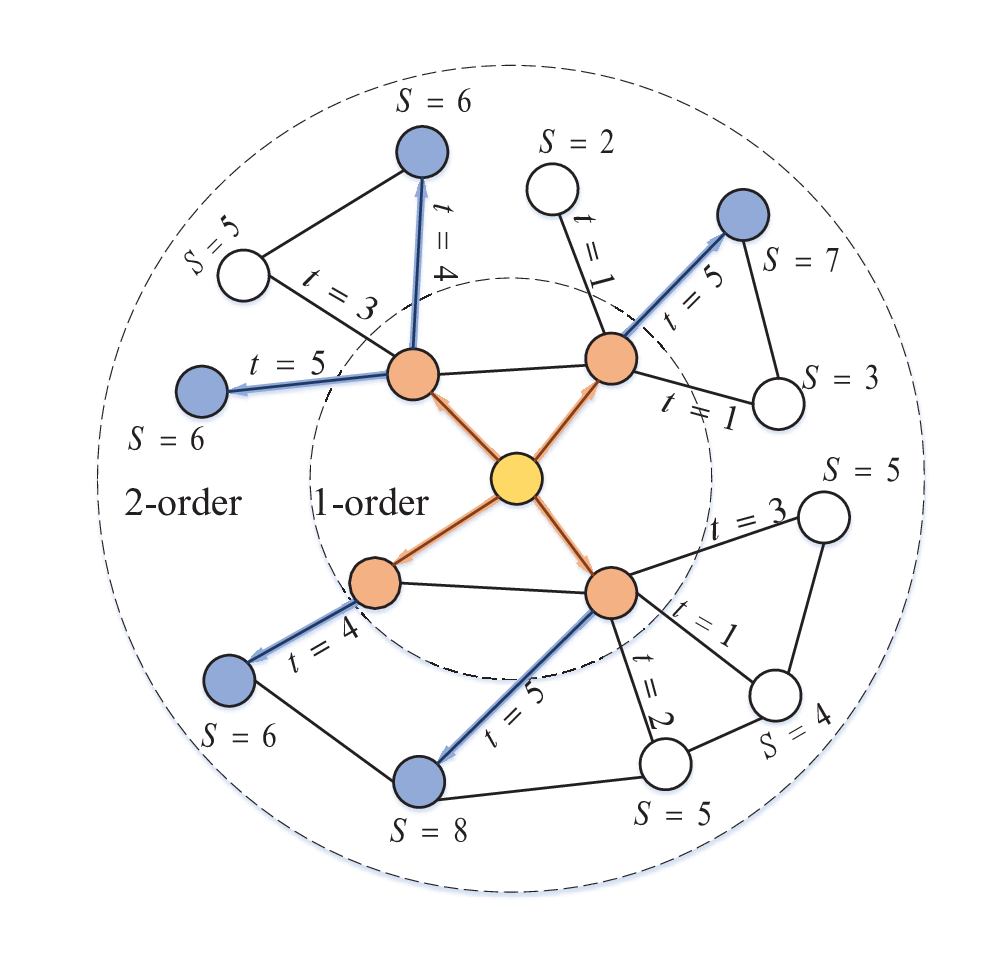
Firstly, all first-order neighbors of are sampled. Since the number of first-order neighbors is usually less than , the second-order or even the higher-order neighbors of may be sampled until the number of candidate nodes is greater than or equal to .
Then, if the number of candidate nodes exceeds , a selection strategy is adopted to select more important candidate nodes into the sampling pool according to their importance score, which is defined as the combination of structural importance score (Eq. 1) and temporal importance score (described below), where is the node id in the sampling path.
The structural importance score is simply defined as the degree of the node:
| (1) |
Actually, can also be defined using other measures such as the eigenvector centrality (Newman 2018) , influence in PageRank (Newman 2018), etc.
The temporal importance score is a normalized largest timestamp of the edge connected to node .
As a result, the importance score of node is denoted as:
| (2) |
where, is the hyperparameter used to balance the influence of structure and time.
An example is shown in Figure 3, where represents the timestamp and represents the importance score. Assuming that , for the yellow central node, its 4 first-order neighbors are first sampled and then its 11 second-order neighbors are also sampled, increasing to 16 nodes in the candidate set. According to Eq. 2, 5 blue nodes with the highest importance score will be saved as the sampling nodes.
Finally, after the nodes are sampled, the time-weighted subgraph and unweighted subgraph of node are obtained referring to the original graph (Jiao et al. 2020), represented by the adjacency matrix and respectively. The edge weight in is the normalization of its latest timestamp. The feature matrix and the adjacency matrix of are:
| (3) |
where, represents the index of the sampled node. is the row-wise (i.e. node-wise) indexed feature matrix. is the row-wise and col-wise indexed adjacency matrix. Similarly, the feature matrix and adjacency matrix of are also obtained.
As a result, the output of the temporal subgraph sampling module for each node includes a time-weighted subgraph and an unweighted subgraph . Both of them will be used in the subsequent contrastive learning task.
3.4. Node and Subgraph Representation
After obtaining and , the encoder and are used to output their representation and , respectively:
| (4) |
For simplicity, both and adopt a one-layer graph convolutional network (GCN) (Kipf and Welling 2017) that can efficiently aggregate neighbor information. Take as an example, the propagation rules are as follows:
| (5) |
where is the adjacency matrix inserted into a self-loop, is the corresponding degree matrix. The non-linear function is the perametric ReLU (PReLU) function (He et al. 2015) and is a learnable linear transformation.
The representation of the central node is then picked out from the representation matrix :
| (6) |
where denotes the pick-out operation.
To facilitate the subsequent contrast learning tasks, the time-weighted subgraph representation and the unweighted subgraph representation are represented by using two readout functions and , respectively.
is a time-aware readout function designed in this paper, which calculates the influence score of any node on the central node (Eq. 7) and then performs a weighted average of node representations to get (Eq. 8).
| (7) |
where, represents the latest interaction timestamp between and , represents the shortest distance between and and is a hyperparameter.
| (8) |
where, is the number of nodes in .
is used to simply average all node representations in the subgraph :
| (9) |
3.5. Temporal Contrastive Learning
Pretext tasks and the generation of positive and negative samples are crucial for self-supervised learning. As mentioned above, the dynamics of neighborhood nodes has greater influence on the central node than that of distant nodes. The pretext task is designed to make the central node strongly correlated to its regional neighbors. In our method, the mutual information of the central node and its corresponding temporal subgraph is maximized.
For the central node , the pretext task is to contrast its real temporal subgraph to its fake temporal subgraph. Specifically, a positive sample, a structural negative sample and a temporal negative sample are constructed for . The positive sample is the time-weighted subgraph representation . The structural negative sample is generated by shuffling the representation set of time-weighted subgraphs, denoted as:
| (10) |
The temporal negative sample is the unweighted subgraph representation , with the purpose to make the node representation closer to the time-weighted subgraph representation and farther away from the unweighted subgraph representation . The temporal contrast information is therefore emphasized.
Finally, the margin triplet loss is used to train the model as it is more favorable for subgraph contrastive learning (Jiao et al. 2020). The margin loss of the structural negative sample is defined as:
| (11) |
where is the sigmoid function and is the margin value. Similarly, the margin loss of the temporal negative sample is defined as:
| (12) |
where is the margin value. As a result, the total loss function of the model is:
| (13) |
where is a hyperparameter to balance two loss.
The process of DySubC is summarized in Algorithm 2.
4. EXPERIMENTS
The following experiments are conducted to evaluate our model from various aspects.
- •
The performance of DynSubC and the related baseline methods in link prediction is compared, thereby reflecting their representation learning ability.
- •
The effectiveness of each proposed time-enhanced module and how it affects the overall model is evaluated.
- •
In the temporal subgraph sampling module, the impact of the subgraph size on the model is explored, and the balance between memory and performance is analyzed.
- •
The sensitivity of the model to hyperparameters is analyzed.
- •
The visualization of node representations obtained by DySubC and Sub-Con is compared.
Before detailing the experimental results and analysis, we start with a brief introduction of the datasets, the experimental settings and the baselines.
4.1. Datasets
For a comprehensive comparison, we use five widely used datasets collected from different types of real networks. The detailed statistics of the datasets are summarized in Table 1.
- •
fb-forum (Opsahl 2013). The dataset is a forum network similar to Facebook, obtained from online social networks. The directed edge means that user and user interacted at time .
- •
soc-sign-bitcoinalpha (Kumar et al. 2016; Kumar et al. 2018). This is a who-trusts-whom network among people who trade using Bitcoin on a platform called Bitcoin Alpha. The directed edge indicates that user trusted user at time .
- •
soc-wiki-elec (Rossi and Ahmed 2015). The dataset contains the administrator election and voting data based on the latest complete dump of Wikipedia page edit history (from January 3, 2008). The directed edge indicates that voted for at time .
- •
ia-movielens-user2tags-10m (Rossi and Ahmed 2015). This bipartite network represents the tagging behaviors of MovieLens users. The nodes represent users and movies. The directed edge means that the user tagged the movie at time.
- •
sx-mathoverflow-c2q (Paranjape et al. 2017). It is a temporal interaction network on the stack exchange website Math Overflow. The directed edge means that user commented on user ’s question at time .
| Dynamic graph | Timespan (days) | ||
|---|---|---|---|
| fb-forum | 899 | 33,720 | 164.49 |
| soc-sign-bitcoinalpha | 3,783 | 24,186 | 1,901.00 |
| soc-wiki-elec | 7,118 | 107,071 | 1,378.34 |
| ia-movielens-user2tags-10m | 16,528 | 95,580 | 1,108.97 |
| sx-mathoverflow-c2q | 16,836 | 203,639 | 2,349.00 |
| fb-forum | soc-sign-bitcoinalpha | soc-wiki-elec | ia-movielens-user2tags-10m | sx-mathoverflow-c2q | ||||||
| AUC | Accuracy | AUC | Accuracy | AUC | Accuracy | AUC | Accuracy | AUC | Accuracy | |
| node2vec | 0.7351 | 0.6703 | 0.7001 | 0.6514 | 0.6877 | 0.6439 | 0.7118 | 0.6477 | 0.7521 | 0.6932 |
| graphSAGE | 0.7465 | 0.6815 | 0.7389 | 0.6887 | 0.7454 | 0.7014 | 0.7648 | 0.6994 | 0.7863 | 0.7258 |
| DGI | 0.8118 | 0.7589 | 0.7948 | 0.7428 | 0.8828 | 0.8127 | 0.8975 | 0.8484 | 0.8392 | 0.7803 |
| Sub-Con | 0.8506 | 0.7802 | 0.8735 | 0.8092 | 0.8784 | 0.8084 | 0.8052 | 0.7321 | 0.8281 | 0.7725 |
| CTDNE | 0.7522 | 0.6897 | 0.7334 | 0.6891 | 0.7225 | 0.6854 | 0.7855 | 0.7234 | 0.8507 | 0.7987 |
| HTNE | 0.7756 | 0.7023 | 0.7365 | 0.6872 | 0.8253 | 0.7673 | 0.8271 | 0.7562 | 0.8429 | 0.7904 |
| DyRep | 0.7592 | 0.6814 | 0.8274 | 0.7684 | 0.8381 | 0.7794 | 0.8395 | 0.7883 | 0.8766 | 0.8237 |
| TGN | 0.8678 | 0.7895 | 0.8375 | 0.7776 | 0.8794 | 0.8116 | 0.8659 | 0.8017 | 0.9371 | 0.8821 |
| DySubC | 0.8861 | 0.8082 | 0.9221 | 0.8457 | 0.9229 | 0.8558 | 0.9524 | 0.8902 | 0.9302 | 0.8791 |
| fb-forum | soc-sign-bitcoinalpha | soc-wiki-elec | ia-movielens-user2tags-10m | sx-mathoverflow-c2q | ||||||
|---|---|---|---|---|---|---|---|---|---|---|
| AUC | Accuracy | AUC | Accuracy | AUC | Accuracy | AUC | Accuracy | AUC | Accuracy | |
| DySubC-S-N-R | 0.8442 | 0.7661 | 0.8967 | 0.8186 | 0.8874 | 0.8264 | 0.9301 | 0.8705 | 0.8815 | 0.8156 |
| DySubC-N-R | 0.8572 | 0.7782 | 0.9149 | 0.8388 | 0.9124 | 0.8462 | 0.9395 | 0.8751 | 0.9017 | 0.8458 |
| DySubC-R | 0.8821 | 0.8051 | 0.9203 | 0.8415 | 0.9218 | 0.8543 | 0.9511 | 0.8877 | 0.9283 | 0.8768 |
| DySubC | 0.8861 | 0.8082 | 0.9221 | 0.8457 | 0.9229 | 0.8558 | 0.9524 | 0.8902 | 0.9302 | 0.8791 |
4.2. Experimental settings
Since the nodes in the above datasets have no features, we use one-hot encoding as the initial features of the node. Considering that the downstream task is link prediction, we first sort the edges in the graph in ascending order of time, using the recent 25% randomly divided as validation set (10%) and test set (15%) and the remaining 75% as the training set. For the recent 25% edges (i.e. positive samples), we randomly sample the same number of negative samples (unconnected node pairs).
For each experiment, the dimension of node representations is set to 128. A simple logistic regression classifier is trained and tested for link prediction using the embedding results. We train the model for 10 times on different data splits and report the average performance for fair evaluation. Consistent with previous work (Rossi et al. 2020; Trivedi et al. 2019; Nguyen et al. 2018; Zuo et al. 2018), we also use AUC and accuracy indicator to evaluate the performance of link prediction.
In training, the Adam optimizer is used with an initial learning rate of 0.001. For all datasets, the size of subgraphs is set to 20. Both the margin value and for the loss function are set to 0.75 and is 0.5.
4.3. Baselines
We use three types of representative baseline methods for comparison: (1) Continuous-time dynamic graph representation learning methods: TGN (Rossi et al. 2020), DyRep (Trivedi et al. 2019), CTDNE (Nguyen et al. 2018) and HTNE (Zuo et al. 2018); (2) State-of-art static graph self-supervised methods: DGI (Velickovic et al. 2019) and Sub-Con (Jiao et al. 2020); (3) Static graph representation learning benchmarks: Node2vec (Grover and Leskovec 2016) and GraphSAGE (Hamilton et al. 2017). Note that when reproducing the codes of different models, we carefully select the reported optimal hyperparameters to ensure a fair comparison.
4.4. Performance on Link Prediction
The comparative results of all methods in link prediction performance are summarized in Table 2. Overall, our proposed model shows a competitive performance. Except that the AUC and accuracy of DySubC is slightly lower than that of TGN on the sx-mathoverflow-c2q dataset, the model is superior to all baselines on the remaining datasets. The possible reason for the good performance of TGN on the sx-mathoverflow-c2q dataset is that its memory module will be more advantageous for datasets with a large time span. The methods that use self-supervised learning (DGI, Sub-Con and DySubC) perform better than methods that do not use self-supervised learning (node2vec and graphSAGE).
More detailed observations and analysis are as follows. Firstly, the performance of our model is significantly higher than static self-supervised graph representation learning methods (i.e. DGI and Sub-Con). Especially on the sx-mathoverflow-c2q dataset, the AUC score of DySubC is nearly 0.9 higher than DGI and 0.1 higher than Sub-Con. It verifies the importance of temporal information for graph representation learning models and the temporal subgraph contrastive method in this paper can effectively capture temporal information. Secondly, on the bipartite graph dataset (i.e., ia-movielens-user2tags-10m), the performance of most continuous-time dynamic graph representation learning methods is poor. In contrast, the DySubC model achieves the best performance, which indicates that our method is more robust and can be applied to different types of graphs. Thirdly, DySubC performs significantly better than other models on soc-sign-bitcoinalpha and ia-movielens-user2tags-10m datasets. These two graphs are relatively sparse, which could cause the deterioration in model performance. However, DySubC may alleviate the above problem caused by the graph sparsity since it learns at the sub-graph level. Finally, the performance of Sub-Con on the ia-movielens-user2tags-10m dataset is poor, probably because its subgraph sampling strategy is a personalized PageRank algorithm (Newman 2018). It may not sample sufficient first-order neighbors, which are particularly important for the central node in the bipartite graph.
4.5. Ablation Studies
In order to further observe the impact of three time-enhanced modules (i.e., temporal subgraph sampling, time-weighted subgraph representation and temporal contrastive learning) of DySubC, we conduct a series of ablation experiments by replacing each of the three modules with the counterpart that does not utilize the time information. The subscript -S represents that the model replaces the temporal subgraph sampling with a subgraph sampling that only uses structural information. The subscript -N means that the model does not use the negative sample for contrastive learning. The subscript -R stands for replacing our designed readout function with a simple average function in time-weighted subgraph representation. It is worth noting that DySubC-S-N-R and Sub-Con (Jiao et al. 2020) are not equivalent, as their subgraph sampling strategies are different.
The ablation results are listed in Table 3. It verifies the effectiveness of each time-enhanced module, which consistently improves the model performance on all datasets. Especially when considering the negative sample , the performance of the model is significantly improved (see the comparative results of DySubC-R and DySubC-N-R). The combination of three modules achieves the best performance. On the sx-mathoverflow-c2q dataset, the final DySubC model gains an improvement of 0.05 AUC score compared to the base model with no time-enhanced module enabled.
4.6. Subgraph Size Analysis
This section studies the impact of the subgraph size in DynSubC on the five datasets. We adjust the subgraph size from 10 to 100 (including the central node), and the evaluation results are shown in Figure 4. Note that in the experiment on ia-movielens-user2tags-10m and sx-mathoverflow-c2q datasets, the maximum subgraph size is set as 50 due to limited computational memory. The corresponding result with size 100 in the figure is approximated by the result with size 50, since the model performance tends to be stable.
As shown in the figure, the model achieves better performance when the size of the subgraph is larger. It is probably because neighborhood nodes contain more structural and temporal information, which helps to obtain a higher quality representation. However, in the fb-forum dataset, the model with the subgraph size 100 performs worse than the model with the subgraph size 50. It may be because the dataset is small in size, a large size subgraph will contain nodes far away from the central node, which could be not beneficial to representation learning. When the size of subgraph is too small (e.g., 10), the performance of the model in all datasets is poor, which indicates that necessary information for learning is lost. When the subgraph size is 20, the model performs quite well on all five datasets and consumes less system memory than the model with a larger subgraph size.

4.7. Sensitivity Analysis
In this section, the sensitivity analysis is conducted on critical hyperparameters in DynSubC, i.e., and , which determine the quality of temporal subgraph sampling and time-weighted subgraph representation. Specifically, the value of is increased from 2 to 20 with the step size 2 and the value of is increased from 0.4 to 3.6 with the step size 0.4.
The stability of the model under the perturbation of the two hyperparameters is observed. The results on the fb-forum dataset are shown in Figure 5. The model performs best when is 10 and is 1.6, both of which are around the median of their respective value ranges. It demonstrates that DynSubC is sensitive to these two hyperparameters. As we mentioned before, is used to balance the structural and temporal information in the subgraph sampling. The result shows that the temporal information is at least as important as structural information when sampling and should be considered. is used to balance the influence of the latest interaction and its distance to the central node. Both are verified to be indispensable in subgraph representation.

4.8. Visualization Analysis
Finally, we use the tSNE algorithm (Maaten and Hinton 2008) to visualize the node representation and the latest interactions obtained by DySubC and Sub-Con. Figure 6 shows the result on the soc-sign-bitcoinalpha dataset. The red lines denote the latest 10 interactions. The visualization result shows that DySubC can better embed the evolutional features of nodes into the representation, so that the latest interacted nodes are also closer in the embedding space compared to Sub-Con, which is a static subgraph contrast method. Moreover, it is observed that the nodes that are recently active are more clustered in the visualization of DySubC than that of Sub-Con. It is consistent with the characteristics of the dataset, that is, users who trust each other are often in a community structure, so they are supposed to be closer in the embedding space.


5. CONCLUSION
In this paper, a novel self-supervised dynamic graph representation learning framework (DySubC) based on temporal subgraph contrast is proposed. The model learns the representation with both structural and temporal information by maximizing the mutual information of the node representation and its temporal subgraph representation. DySubC proposes three time-enhanced modules, which can not only sample more effective subgraphs, but also learn better representation by temporal contrast loss. The effectiveness of DySubC compared with related graph contrast learning methods and dynamic graph representation learning methods is demonstrated by empirical evaluation on multiple datasets. The success of DySubC provides an insight for the future study on continuous-time graph representation learning.
References
- (1)
- Chen et al. (2018) Jie Chen, Tengfei Ma, and Cao Xiao. 2018. FastGCN: Fast Learning with Graph Convolutional Networks via Importance Sampling. In 6th International Conference on Learning Representations, ICLR 2018, Vancouver, BC, Canada, April 30 - May 3, 2018, Conference Track Proceedings. OpenReview.net. https://openreview.net/forum?id=rytstxWAW
- Chen et al. (2020) Ting Chen, Simon Kornblith, Mohammad Norouzi, and Geoffrey E. Hinton. 2020. A Simple Framework for Contrastive Learning of Visual Representations. 119 (2020), 1597–1607. http://proceedings.mlr.press/v119/chen20j.html
- Goyal et al. (2018) Palash Goyal, Nitin Kamra, Xinran He, and Yan Liu. 2018. DynGEM: Deep Embedding Method for Dynamic Graphs. CoRR abs/1805.11273 (2018). arXiv:1805.11273 http://arxiv.org/abs/1805.11273
- Grover and Leskovec (2016) Aditya Grover and Jure Leskovec. 2016. node2vec: Scalable Feature Learning for Networks. (2016), 855–864. https://doi.org/10.1145/2939672.2939754
- Hamilton et al. (2017) William L. Hamilton, Zhitao Ying, and Jure Leskovec. 2017. Inductive Representation Learning on Large Graphs. (2017), 1024–1034. https://proceedings.neurips.cc/paper/2017/hash/5dd9db5e033da9c6fb5ba83c7a7ebea9-Abstract.html
- Hassani and Ahmadi (2020) Kaveh Hassani and Amir Hosein Khas Ahmadi. 2020. Contrastive Multi-View Representation Learning on Graphs. 119 (2020), 4116–4126. http://proceedings.mlr.press/v119/hassani20a.html
- He et al. (2015) Kaiming He, Xiangyu Zhang, Shaoqing Ren, and Jian Sun. 2015. Delving Deep into Rectifiers: Surpassing Human-Level Performance on ImageNet Classification. (2015), 1026–1034. https://doi.org/10.1109/ICCV.2015.123
- Jiao et al. (2020) Yizhu Jiao, Yun Xiong, Jiawei Zhang, Yao Zhang, Tianqi Zhang, and Yangyong Zhu. 2020. Sub-graph Contrast for Scalable Self-Supervised Graph Representation Learning. (2020), 222–231. https://doi.org/10.1109/ICDM50108.2020.00031
- Jing and Tian (2021) Longlong Jing and Yingli Tian. 2021. Self-Supervised Visual Feature Learning With Deep Neural Networks: A Survey. IEEE Trans. Pattern Anal. Mach. Intell. 43, 11 (2021), 4037–4058. https://doi.org/10.1109/TPAMI.2020.2992393
- Kipf and Welling (2017) Thomas N. Kipf and Max Welling. 2017. Semi-Supervised Classification with Graph Convolutional Networks. (2017). https://openreview.net/forum?id=SJU4ayYgl
- Kumar et al. (2018) Srijan Kumar, Bryan Hooi, Disha Makhija, Mohit Kumar, Christos Faloutsos, and V. S. Subrahmanian. 2018. REV2: Fraudulent User Prediction in Rating Platforms. In Proceedings of the Eleventh ACM International Conference on Web Search and Data Mining, WSDM 2018, Marina Del Rey, CA, USA, February 5-9, 2018, Yi Chang, Chengxiang Zhai, Yan Liu, and Yoelle Maarek (Eds.). ACM, 333–341. https://doi.org/10.1145/3159652.3159729
- Kumar et al. (2016) Srijan Kumar, Francesca Spezzano, V. S. Subrahmanian, and Christos Faloutsos. 2016. Edge Weight Prediction in Weighted Signed Networks. In IEEE 16th International Conference on Data Mining, ICDM 2016, December 12-15, 2016, Barcelona, Spain, Francesco Bonchi, Josep Domingo-Ferrer, Ricardo Baeza-Yates, Zhi-Hua Zhou, and Xindong Wu (Eds.). IEEE Computer Society, 221–230. https://doi.org/10.1109/ICDM.2016.0033
- Liao et al. (2019) Renjie Liao, Zhizhen Zhao, Raquel Urtasun, and Richard S. Zemel. 2019. LanczosNet: Multi-Scale Deep Graph Convolutional Networks. (2019). https://openreview.net/forum?id=BkedznAqKQ
- Liu et al. (2020) Xiao Liu, Fanjin Zhang, Zhenyu Hou, Zhaoyu Wang, Li Mian, Jing Zhang, and Jie Tang. 2020. Self-supervised Learning: Generative or Contrastive. CoRR abs/2006.08218 (2020). arXiv:2006.08218 https://arxiv.org/abs/2006.08218
- Liu et al. (2021) Yixin Liu, Shirui Pan, Ming Jin, Chuan Zhou, Feng Xia, and Philip S. Yu. 2021. Graph Self-Supervised Learning: A Survey. CoRR abs/2103.00111 (2021). arXiv:2103.00111 https://arxiv.org/abs/2103.00111
- Maaten and Hinton (2008) van der Laurens Maaten and Geoffrey Hinton. 2008. Visualizing Data using t-SNE. JOURNAL OF MACHINE LEARNING RESEARCH (2008), 2579–2605.
- Newman (2001) M. E. J. Newman. 2001. The structure of scientific collaboration networks. Proceedings of the National Academy of Sciences 98, 2 (2001), 404–409. https://doi.org/10.1073/pnas.98.2.404 arXiv:https://www.pnas.org/content/98/2/404.full.pdf
- Newman (2018) Mark E. J. Newman. 2018. Networks: An Introduction (Second Edition). Oxford University Press.
- Nguyen et al. (2018) Giang Hoang Nguyen, John Boaz Lee, Ryan A. Rossi, Nesreen K. Ahmed, Eunyee Koh, and Sungchul Kim. 2018. Continuous-Time Dynamic Network Embeddings. (2018), 969–976. https://doi.org/10.1145/3184558.3191526
- Opsahl (2013) Tore Opsahl. 2013. Triadic closure in two-mode networks: Redefining the global and local clustering coefficients. Soc. Networks 35, 2 (2013), 159–167. https://doi.org/10.1016/j.socnet.2011.07.001
- Paranjape et al. (2017) Ashwin Paranjape, Austin R. Benson, and Jure Leskovec. 2017. Motifs in Temporal Networks. (2017), 601–610. https://doi.org/10.1145/3018661.3018731
- Pareja et al. (2020) Aldo Pareja, Giacomo Domeniconi, Jie Chen, Tengfei Ma, Toyotaro Suzumura, Hiroki Kanezashi, Tim Kaler, Tao B. Schardl, and Charles E. Leiserson. 2020. EvolveGCN: Evolving Graph Convolutional Networks for Dynamic Graphs. (2020), 5363–5370. https://aaai.org/ojs/index.php/AAAI/article/view/5984
- Peng et al. (2020) Zhen Peng, Wenbing Huang, Minnan Luo, Qinghua Zheng, Yu Rong, Tingyang Xu, and Junzhou Huang. 2020. Graph Representation Learning via Graphical Mutual Information Maximization. (2020), 259–270. https://doi.org/10.1145/3366423.3380112
- Perozzi et al. (2014) Bryan Perozzi, Rami Al-Rfou, and Steven Skiena. 2014. DeepWalk: online learning of social representations. (2014), 701–710. https://doi.org/10.1145/2623330.2623732
- Qiu et al. (2020) Jiezhong Qiu, Qibin Chen, Yuxiao Dong, Jing Zhang, Hongxia Yang, Ming Ding, Kuansan Wang, and Jie Tang. 2020. GCC: Graph Contrastive Coding for Graph Neural Network Pre-Training. (2020), 1150–1160. https://doi.org/10.1145/3394486.3403168
- Qu et al. (2019) Meng Qu, Yoshua Bengio, and Jian Tang. 2019. GMNN: Graph Markov Neural Networks. 97 (2019), 5241–5250. http://proceedings.mlr.press/v97/qu19a.html
- Rossi et al. (2020) Emanuele Rossi, Ben Chamberlain, Fabrizio Frasca, Davide Eynard, Federico Monti, and Michael M. Bronstein. 2020. Temporal Graph Networks for Deep Learning on Dynamic Graphs. CoRR abs/2006.10637 (2020). arXiv:2006.10637 https://arxiv.org/abs/2006.10637
- Rossi and Ahmed (2015) Ryan A. Rossi and Nesreen K. Ahmed. 2015. The Network Data Repository with Interactive Graph Analytics and Visualization. In Proceedings of the Twenty-Ninth AAAI Conference on Artificial Intelligence, January 25-30, 2015, Austin, Texas, USA, Blai Bonet and Sven Koenig (Eds.). AAAI Press, 4292–4293. http://www.aaai.org/ocs/index.php/AAAI/AAAI15/paper/view/9553
- Sankar et al. (2020) Aravind Sankar, Yanhong Wu, Liang Gou, Wei Zhang, and Hao Yang. 2020. DySAT: Deep Neural Representation Learning on Dynamic Graphs via Self-Attention Networks. (2020), 519–527. https://doi.org/10.1145/3336191.3371845
- Tang et al. (2015) Jian Tang, Meng Qu, Mingzhe Wang, Ming Zhang, Jun Yan, and Qiaozhu Mei. 2015. LINE: Large-scale Information Network Embedding. (2015), 1067–1077. https://doi.org/10.1145/2736277.2741093
- Trivedi et al. (2019) Rakshit Trivedi, Mehrdad Farajtabar, Prasenjeet Biswal, and Hongyuan Zha. 2019. DyRep: Learning Representations over Dynamic Graphs. (2019). https://openreview.net/forum?id=HyePrhR5KX
- Vaswani et al. (2017) Ashish Vaswani, Noam Shazeer, Niki Parmar, Jakob Uszkoreit, Llion Jones, Aidan N. Gomez, Lukasz Kaiser, and Illia Polosukhin. 2017. Attention is All you Need. (2017), 5998–6008. https://proceedings.neurips.cc/paper/2017/hash/3f5ee243547dee91fbd053c1c4a845aa-Abstract.html
- Velickovic et al. (2018) Petar Velickovic, Guillem Cucurull, Arantxa Casanova, Adriana Romero, Pietro Liò, and Yoshua Bengio. 2018. Graph Attention Networks. https://openreview.net/forum?id=rJXMpikCZ
- Velickovic et al. (2019) Petar Velickovic, William Fedus, William L. Hamilton, Pietro Liò, Yoshua Bengio, and R. Devon Hjelm. 2019. Deep Graph Infomax. https://openreview.net/forum?id=rklz9iAcKQ
- Wang et al. (2016) Daixin Wang, Peng Cui, and Wenwu Zhu. 2016. Structural Deep Network Embedding. (2016), 1225–1234. https://doi.org/10.1145/2939672.2939753
- Wu et al. (2019) Felix Wu, Amauri H. Souza Jr., Tianyi Zhang, Christopher Fifty, Tao Yu, and Kilian Q. Weinberger. 2019. Simplifying Graph Convolutional Networks. 97 (2019), 6861–6871. http://proceedings.mlr.press/v97/wu19e.html
- Zaremba et al. (2014) Wojciech Zaremba, Ilya Sutskever, and Oriol Vinyals. 2014. Recurrent Neural Network Regularization. CoRR abs/1409.2329 (2014). arXiv:1409.2329 http://arxiv.org/abs/1409.2329
- Zhou et al. (2018) Le-kui Zhou, Yang Yang, Xiang Ren, Fei Wu, and Yueting Zhuang. 2018. Dynamic Network Embedding by Modeling Triadic Closure Process. (2018), 571–578. https://www.aaai.org/ocs/index.php/AAAI/AAAI18/paper/view/16572
- Zhu et al. (2020) Yanqiao Zhu, Yichen Xu, Feng Yu, Qiang Liu, Shu Wu, and Liang Wang. 2020. Deep Graph Contrastive Representation Learning. CoRR abs/2006.04131 (2020). arXiv:2006.04131 https://arxiv.org/abs/2006.04131
- Zhu et al. (2021) Yanqiao Zhu, Yichen Xu, Feng Yu, Qiang Liu, Shu Wu, and Liang Wang. 2021. Graph Contrastive Learning with Adaptive Augmentation. (2021), 2069–2080. https://doi.org/10.1145/3442381.3449802
- Zuo et al. (2018) Yuan Zuo, Guannan Liu, Hao Lin, Jia Guo, Xiaoqian Hu, and Junjie Wu. 2018. Embedding Temporal Network via Neighborhood Formation. (2018), 2857–2866. https://doi.org/10.1145/3219819.3220054