Geometric energy transfer in two-component systems

Exposing a molecule to a visible or UV electromagnetic pulse excites primarily the electronic degrees of freedom. On a longer time scale, the electrons transfer energy to the nuclei. While energy transfer can be evaluated with knowledge of the electron-nuclear wave function, given a choice of nuclear subsystem, to gain deeper insight into excited state molecular dynamics, optimize control of molecular motion and bond breaking, and engineer molecular scale mechanical motion, it would be valuable to have a formula expressing the energy transfer in terms of simple fundamental quantities.

Using the exact factorization (EF) formalism Gidopoulos and Gross 2014; Abedi et al. 2010, which involves the factorization of a two-component wave function into a product of marginal and conditional amplitudes Hunter 1975, we have derived Ehrenfest identities Li et al. 2019 for the time rate of change of the kinetic energy, momentum and angular momentum of the nuclear subsystem. By evaluating the commutators in the Heisenberg equations of motion, we found that a novel quantum mechanical force operator appeared in all three identities. In terms of this force operator, all three identities could be put in a form directly analogous to the classical equations of motion $dE/dt=\mathbf{F}\cdot\mathbf{v}$, $d\mathbf{P}/dt=\mathbf{F}$ and $d\mathbf{L}/dt=\mathbf{R}\times\mathbf{F}$.

One wrinkle in those results was the fact that the classical force-times-velocity form could only be achieved for the rate of change of one part of the nuclear kinetic energy, namely the term

where $|\chi\rangle$ is the nuclear wave function that satisfies the effective Schrödinger equation

of the exact factorization method; $R$ denotes the set $\{\mathbf{R}_{i}\}$ of $N_{n}$ nuclear coordinates. $T_{n,marg}$ is the kinetic energy of a fictitious closed quantum system acted upon by scalar and vector potentials $\mathcal{E}(R,t)$ and $\mathbf{A}_{i}(R,t)$ (defined below). In other words, it is simply the kinetic energy one would write down if one were given the Schrödinger equation (2) but not told it describes only one component of a two-component system. Since $\chi$ is the marginal probability amplitude for the nuclear component of a system of electrons and nuclei, we call $T_{n,marg}$ the marginal nuclear kinetic energy.

The closed system described by equation (2) reproduces the true $N_{n}$-body density and $N_{n}$-body current density of the nuclear subsystem, but it is fictitious in the sense that off-diagonal elements of the nuclear density matrix and hence nonlocal observables of the nuclear subsystem cannot be calculated directly from the wave function $\chi$. A prime example is the true nuclear kinetic energy as obtained from the full wave function $|\Psi\rangle$ which obeys the identity Abedi et al. 2012; Agostini et al. 2015

where the additional contribution is

with $\mathbf{A}_{i}=\mathrm{Re}\langle\Phi|\mathbf{P}_{i}\Phi\rangle$ and $\Phi(r|R)=\Psi(r,R)/\chi(R)$ being the electronic wavefunction conditional on $R$. The Ehrenfest identity of Ref. Li et al. 2019 provides a straightforward way to calculate $dT_{n,marg}/dt$ but gives no information about $dT_{n,geo}/dt$.

Our main result is an exact identity for $dT_{n,geo}/dt$, expressed in terms of primitive quantities. An interesting outcome of the derivation is the appearance of a new rank-3 quantum geometric quantity that cannot be expressed in terms of lower-rank quantities.

The integrand of (4) has geometric significance itself, as it can be expressed Requist et al. 2016; Requist and Gross 2016 in terms of a tensor contraction between $\mathcal{I}^{\mu\nu}$, a symmetric inverse inertia tensor, and a Riemannian metric Provost and Vallee 1980

on nuclear configuration space, i.e. the manifold $\mathcal{Q}$ with generalized coordinates $\{Q^{\mu}\}$ collectively denoted $Q$. Thus, we have

which we call the geometric part of the nuclear kinetic energy. As all quantities except $\mathcal{I}^{\mu\nu}$ are time dependent, we suppress the time argument here and hereafter. In (5) and (6), we have switched to a tensor calculus notation, i.e. subscripts/superscripts correspond to the covariant/contravariant indices of a tensor on $\mathcal{Q}$, and we have generalized to a Watsonian kinetic energy operator $\hat{T}_{n}=(1/2)\mathcal{I}^{\mu\nu}P_{\mu}P_{\nu}$ Watson 1968 with $P_{\mu}=-i\partial/\partial Q^{\mu}$ and an implicit summation convention. The metric in equation (5) is the EF counterpart of the quantum metric tensor originally studied in the Born-Oppenheimer (BO) approximation Berry 1989; Shapere and Wilczek 1989; Berry and Lim 1990; Berry and Robbins 1993. The quantum metric tensor has recently attracted attention in condensed matter physics, where its applications are too numerous to cite here.

The usual laboratory frame kinetic energy operator, cf. equation (3), is a special case of the Watsonian kinetic energy, in which the set of $Q^{\mu}$ is $\{R_{1x},R_{1y},R_{1z},R_{2x},R_{2y},R_{2z},\ldots\}$ and $\mathcal{I}^{\mu\nu}$ is diagonal and $Q^{\mu}$-independent, i.e. $\mathcal{I}^{\mu\nu}=\mathcal{I}^{i\alpha,j\beta}=M_{i}^{-1}\delta_{ij}\delta_{\alpha\beta}$ with $i$ labeling the nucleus and $\alpha=x,y,z$. The Watson form encompasses two additional cases: (1) an isolated molecule after removing the center-of-mass and overall rotational coordinates Sutcliffe 2000; and (2) a system described by a distinguished set of relevant collective coordinates. The phonon modes of a crystalline solid described with Born-von Karman boundary conditions are an example of case (2) in which $Q^{\mu}$ comprise the normal mode amplitudes $U_{\mathbf{q}\lambda}$ with quasimomentum $\mathbf{q}$ and branch $\lambda$, $\mathcal{I}^{\mu\nu}=\mathcal{I}^{\mathbf{q}\lambda,\mathbf{q}^{\prime}\lambda^{\prime}}=\mathcal{M}_{\mathbf{q}\lambda}^{-1}\delta_{\mathbf{q},-\mathbf{q}}\delta_{\lambda,\lambda^{\prime}}$ is off-diagonal and $\mathcal{M}_{\mathbf{q}\lambda}$ is the effective mass of the normal mode Requist et al. 2019. In case (2), $\mathcal{I}^{\mu\nu}$ will be $Q^{\mu}$-dependent when $\mathcal{Q}$ is non-Euclidean, which can arise e.g. in an approximate reduced description in terms of a restricted set of collective coordinates. In the case of an isolated molecule in which only the center-of-mass coordinate is removed, it is always possible to choose translationally-invariant coordinates such that $\mathcal{I}^{\mu\nu}$ is $Q^{\mu}$-independent Requist and Gross 2016; Sutcliffe 2000; such an $\mathcal{I}^{\mu\nu}$ is generally non-diagonal but can be further diagonalized. Here, for simplicity, we assume $\mathcal{I}^{\mu\nu}$ is $Q^{\mu}$-independent but not necessarily diagonal.

To derive an identity for $dT_{n,geo}/dt$ that does not invoke the BO approximation, we make use of the exact factorization formalism Hunter 1975; Gidopoulos and Gross 2014; Abedi et al. 2010, the essential elements of which we briefly review here.

Starting from the full wavefunction $\Psi(q,Q)=\langle q,Q|\Psi\rangle$, where $q$ and $Q$ denote the sets of electronic and nuclear coordinates, one defines the nuclear wavefunction

which is the marginal probability amplitude corresponding to the marginal probability

and the arbitrary gauge $\lambda(Q)$. The conditional electronic wavefunction

depends parametrically on $Q$ and satisfies the equation

where $\hat{H}^{BO}=\hat{H}-\hat{T}_{n}$ and $\mathcal{E}(Q)=\langle\Phi(Q)|\hat{H}^{BO}|\Phi(Q)\rangle+\mathcal{E}_{geo}(Q)$ with $\mathcal{E}_{geo}(Q)=(1/2)\mathcal{I}^{\mu\nu}g_{\mu\nu}$; $\hat{H}$ is the usual nonrelativistic molecular Hamiltonian in atomic units. Time and other arguments of functions will often be suppressed.

Starting from equation (6), we obtain

where $J^{\mu}$ is the nuclear current density

In the second line of equation (11), we have used the continuity equation, and in the third line, we have performed integration by parts and assumed that the boundary term vanishes; this is generally true for finite systems. Focusing on $\mathcal{E}_{geo}=(1/2)\mathcal{I}^{\mu\nu}g_{\mu\nu}$ in the second term and noting that $\mathcal{I}^{\mu\nu}$ is time-independent, our first step is to evaluate $\partial g_{\mu\nu}/\partial t$:

After contraction with $\mathcal{I}^{\mu\nu}$, these two terms give equal contributions to $\partial_{t}\mathcal{E}_{geo}$. There are no $\partial_{t}A_{\mu}$ contributions because $\mathrm{Re}\langle\Phi|(P_{\mu}-A_{\mu})\Phi\rangle=0$. The terms on the right-hand side of equation (10) give the following contributions to the first term in equation (13):

The (1a) term can be put in various forms but none is simpler than the others. The second term on the right-hand side of $\partial g_{\mu\nu}^{(1a)}/\partial t$ vanishes upon contraction with the symmetric tensor $\mathcal{I}^{\mu\nu}$ because

is real. Turning to the (1b) term and moving $(P_{\nu}-A_{\nu})$ into the bra, we obtain

The second term drops out upon contraction with the symmetric tensor $\mathcal{I}^{\mu\nu}$ because

is real. Therefore, the contribution of the (1b) term to $\partial\mathcal{E}_{geo}/\partial t$ is

where we defined

a manifestly gauge invariant quantity that will be examined in section V.

For the (1c) term, we obtain

The first term simplifies to

where we introduced the definition

The second term of equation (20) gives

where $B_{\mu\nu}=\partial_{\mu}A_{\nu}-\partial_{\nu}A_{\mu}$ is the Berry curvature. Summing equations (21) and (23) and contracting with $\frac{1}{2}\mathcal{I}^{\mu\nu}$, we obtain

where we used equation (47), derived in the section V, to relate $D_{\mu\nu\tau}$ to derivatives of $g_{\mu\nu}$, and hence to $\partial_{\tau}\mathcal{E}_{geo}$. The antisymmetry of $B_{\mu\nu}$ makes the contribution from the second term of equation (23) vanish. The second term of equation (24) will be seen to cancel with the first term of equation (11).

Putting equations (14), (18) and (24) together, we obtain

Substituting this into equation (11) yields the final result

We used the identity

to combine the second and third terms of equation (25), after contraction with $\mathcal{I}^{\mu\nu}$, into the divergence of the vector field

whose volume integral, converted into a surface integral via Gauss’s theorem, generally vanishes for finite systems.

We illustrate the identity (26) for an exactly solvable one-dimensional model with two electronic states. The Schrödinger equation is

Our strategy is to reverse engineer the functions $h_{0}(x,t)$, $h_{1}(x,t)$ and $h_{3}(x,t)$ such that the dynamics lead to a state

with a gaussian nuclear density

that undergoes damped oscillations determined by the functions

Substituting into equation (IV), leads to the following equations:

where subscripts denote partial differentiation, e.g. $\alpha_{x}=\partial_{x}\alpha$. The first equation is equivalent to the continuity equation $\partial_{t}|\chi|^{2}=-\partial_{x}J$ with the nuclear current density

and vector potential

With $|\chi(x,t)|^{2}$ given by equation (33), we have

Defining $w=\cos\theta$, we choose a state $\Psi(x,t)$ with

The Hamiltonian parameters that follow from equation (35) are

The identity in equation (26), adapted to the present model, is

The geometric quantities needed to evaluate the right-hand side are

and for completeness we also record

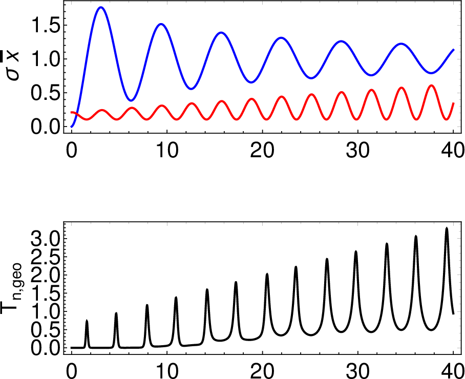
Using the above formulas, we have numerically verified Eq. (41) for $\eta=0.1$, $M=10$ a.u. and $\gamma=40$. The functions $\overline{x}(t)$ and $\sigma(t)$ defining the damped oscillations and the time dependence of $T_{n,geo}$ are shown in Fig. 1.

Here we briefly investigate some properties of the rank-3 quantities $C_{\mu\nu\tau}$ and $D_{\mu\nu\tau}$ that appeared in the last section. Beginning with $D_{\mu\nu\tau}$, we can show that

Thus, $D_{\mu\nu\tau}$ is symmetric with respect to interchange of its second two indices. To further simplify $D_{\mu\nu\tau}$, we derive the following identity:

Taking the real part, we find

With this identity and equation (44), we obtain

Thus, $D_{\mu\nu\tau}$ has been expressed in terms of $g_{\mu\nu}$. In fact, we have

where $\Gamma_{\mu\nu\tau}$ is the Christoffel symbol of the first kind in classical Riemannian geometry.

Turning to $C_{\mu\nu\tau}$, we find the expression

This is also symmetric with respect to the interchange of the second two indices. However, due to the presence of the irreducible third-order quantity $\mathrm{Im}\langle\partial_{\mu}\Phi|\partial_{\nu}\partial_{\tau}\Phi\rangle$, $C_{\mu\nu\tau}$ cannot be expressed in terms of lower-order geometric quantities and their derivatives.

We derived an identity for the rate that energy is transferred to $T_{n,geo}$, the so-called geometric part of the nuclear kinetic energy. This is the part that derives from the gradient with respect to a nuclear coordinate acting on the parametric dependence of an electronic wave function, the latter arising from the factorization of the full wave function. Our identity complements the Ehrenfest-like identity previously derived Li et al. 2019 for $dT_{n,marg}/dt$, the “marginal” part of the nuclear kinetic energy.

Ehrenfest identities for the expectation values of position and momentum resemble Newton’s laws. Similarly, the Ehrenfest-like identity for $dT_{n,marg}/dt$ has a suggestive force-times-velocity form, paralleling the classical formula for the rate of work done by a force, and therefore appears to lend itself to a classical interpretation of the nuclear motion. Indeed, the terms that appear in the force operator have a close resemblance to the corresponding terms in the force on classical nuclei Agostini et al. 2014; Abedi et al. 2014.

It is not yet clear if identity (26) for $dT_{n,geo}/dt$ has a simple classical interpretation. We have not been able to put it in a force-times-velocity form. In the course of evaluating $dT_{n,geo}/dt$, we derived the equation of motion for the quantum metric $g_{\mu\nu}$. This equation involves a new quantity, the rank-3 geometric quantity $C_{\mu\nu\tau}$, which appears to be a purely quantum object.

Putting together the identities for $dT_{n,marg}/dt$ and $dT_{n,geo}/dt$ allow us to calculate the total rate of change of the nuclear kinetic energy. It is hoped that these identities and the insights derived from them will help scientists control energy transfer in quantum systems.

References

• Gidopoulos and Gross (2014) N. I. Gidopoulos and E. K. U. Gross, Phil. Trans. Roy. Soc. A 372, 20130059 (2014).
• Abedi et al. (2010) A. Abedi, N. T. Maitra, and E. K. U. Gross, Phys. Rev. Lett. 105, 123002 (2010).
• Hunter (1975) G. Hunter, Int. J. Quantum Chem. 9, 237 (1975).
• Li et al. (2019) C. Li, R. Requist, and E. K. U. Gross, “Energy, momentum and angular momentum transfer between electrons and nuclei,” arxiv:1908.04077v1 (2019).
• Abedi et al. (2012) A. Abedi, N. T. Maitra, and E. K. U. Gross, J. Chem. Phys. 137, 22A530 (2012).
• Agostini et al. (2015) F. Agostini, A. Abedi, Y. Suzuki, S. K. Min, N. T. Maitra, and E. K. U. Gross, J. Chem. Phys. 142, 084303 (2015).
• Requist et al. (2016) R. Requist, F. Tandetzky, and E. K. U. Gross, Phys. Rev. A 93, 042108 (2016).
• Requist and Gross (2016) R. Requist and E. K. U. Gross, Phys. Rev. Lett. 117, 193001 (2016).
• Provost and Vallee (1980) J. P. Provost and G. Vallee, Commun. Math. Phys. 76, 289 (1980).
• Watson (1968) J. K. G. Watson, Molec. Phys. 15, 479 (1968).
• Berry (1989) M. V. Berry, “The quantum phase, five years after,” (1989) pp. 7–28, in ref. Shapere and Wilczek 1989.
• Shapere and Wilczek (1989) A. Shapere and F. Wilczek, eds., Geometric phases in physics (World Scientific, Singapore, 1989).
• Berry and Lim (1990) M. V. Berry and R. Lim, J. Phys. A: Math. Gen 23, L655 (1990).
• Berry and Robbins (1993) M. V. Berry and J. M. Robbins, Proc. R. Soc. Lond. A 442, 641 (1993).
• Sutcliffe (2000) B. T. Sutcliffe, Adv. Chem. Phys. 114, 97 (2000).
• Requist et al. (2019) R. Requist, C. R. Proetto, and E. K. U. Gross, Phys. Rev. B 99, 165136 (2019).
• Agostini et al. (2014) F. Agostini, A. Abedi, and E. K. U. Gross, J. Chem. Phys. 141, 214101 (2014).
• Abedi et al. (2014) A. Abedi, F. Agostini, and E. K. U. Gross, Europhys. Lett. 106, 33001 (2014).