Model-free Bootstrap Prediction Regions for Multivariate Time Series
Abstract
In [3], a model-free bootstrap(MFB) paradigm was proposed for generating prediction intervals of univariate, (locally) stationary time series. Theoretical guarantees for this algorithm was resolved in [11] under stationarity and weak dependence condition. Following this line of work, here we extend MFB for predictive inference under a multivariate time series setup. We describe two algorithms, the first one works for a particular class of time series under any fixed dimension ; the second one works for a more generalized class of time series under low-dimensional setting. We justify our procedure through theoretical validity and simulation performance.
1 Introduction
Time series forecasting(prediction) is widely applicable in many different fields where the prediction is carried out by conditioning on previous observations. Traditional approaches for time series prediction often rely on a parametric model assumption that can describe the explicit dependence relations of the data. The space of viable time series models that have been studied in the past is huge, therefore the search of good models that can describe the data requires both good understanding of domain knowledge as well as statistical expertise in order to execute model fitting and goodness-of-fit tests.
In a recent monograph, [9] proposed the idea of model-free prediction in the context of regression and time series problems. The idea behind it is to find a one-to-one transform that takes the original data into a new sequence of data that are i.i.d.(independent and identically distributed), then the (inverse) transform along with resampling in the i.i.d. world can be combined to construct both valid point predictors and prediction intervals. Following this, [3] proposed a model-free bootstrap(MFB) algorithm for generating prediction intervals for locally stationary time series that outperforms model-based approach. This algorithm was further studied in [11] under stationary weakly-dependent setting, where bootstrap validity was proved for both prediction interval and confidence intervals for linear statistics and spectral density. In this paper, we extend the model-free bootstrap algorithm of [11] for prediction regions of multivariate time series. We demonstrate the effectiveness of the algorithm by both showing theoretical bootstrap validity and also numerical simulations.
2 Description of algorithm
2.1 Models of interest
Let represent a -dimensional time series. We consider to be from one of the following models:
Model 1: Let be strictly monotone, continuous functions. is a purely non-deterministic, strictly stationary Gaussian process. satisfies
| (1) |
Model 1 is nothing more than a multivariate analog of the class of time series models studied in [11]. Interestingly, it also has connection with copula models for multivariate time series, which we will investigate later. Let us introduce a second class of model:
Model 2: Let be strictly monotone(increasing) functions whose parameters also depend on the previous dimensional entries of : , with the exception of , where is a deterministic function. The time series are defined sequentially in dimensional order in the following manner:
| (2) | ||||
Model 2 is more complicated than model 1 in that we allow for the parameters of subsequent transfer functions to be dependent on previous entries of . Model 1 can be recovered by setting .
Because of the monotonicity of transfer functions, the map is invertible for both models, thus the information set generated by is equivalent to the one generated by , i.e.,
2.2 Connection to copula-based models
Another active line of research for forecasting multivariate time series involves utilizing a copula representation. By Skyler’s theorem, an arbitrary time series can be fully described by the conditional distributions of , and a conditional copula function such that ,
The copula representation offers an approach to decorrelate spatial dependence and serial dependence. Note that in the econometrics literature, the conditional distribution of each dimension are often assumed to be fixed, i.e., , to guarantee effectiveness of valid statistical procedures, see [7]. One of the most famous copulas is the Gaussian copula: a centered dimensional Gaussian random vector with correlation matrix has distribution function
| (3) |
where with ; and is the Gaussian copula with correlation matrix . Generalizing this to the case of a stationary Gaussian processes denoted by , since the conditional distribution of is multivariate normal, it can be fully represented by the Gaussian copula (3) above, where will be the correlation matrix of the conditional normal distribution. Thus .
Another well known fact is that the copula of a joint distribution stays unchanged under monotone function transformations of each marignal random variable. To put it under the setup of model (1) and assume that ,
where is the conditional Gaussian copula of . Thus, the time series of model 1 inherits the same conditional copula as the Gaussian process . is also referred to as the Gaussian copula process, see [12]. However, this does not apply to the case of model 2 where the transfer function parameters depends on other indices of . Therefore, model 2 can be more complicated in that the conditional copula function can go beyond the Gaussian copula.
Notably, the model-free bootstrap to be introduced in the next section shares the same spirit of the semi-parametric method (cf [7] for more details) for copula process prediction. To elaborate, the model-free bootstrap under model (1) requires both estimation of the marginal CDFs via nonparametric method, as well as consistent estimation for the autocovariance structure of the underlying Gaussian process. Similarly, the semi-parametric approach in [7] assumes general distributions for the CDF which are estimated via nonparametric methods, while the copula function is assumed to belong to a particular parametric family(e.g, Gaussian), and then estimation for the copula is carried out parametrically.
2.3 The model-free bootstrap algorithm
The model-free bootstrap of [9] offers a general principle for conducting bootstrap resampling procedure for parameter inference and predictive inference under regression or time series setups. In the univariate time series setting, the algorithm relies on an invertible transform between a length time series data , and a set of i.i.d. random variables , where is sample size adaptive. For parameter inference, let be the parameter of interest which is estimated by some statistic . The model-free bootstrap is first performed in the space of i.i.d. random variables to generate , and then we use the to get bootstrap samples . Then the distribution of can be approximated by , where is calculated based on the bootstrap sample.
Predictive inference is in a more difficult situation, as valid predictions should be carried out conditioning on the entire observed series . First of all, we need a notion called the predictive root, an analog to the pivot random variable in previous setting, which is defined as
where is the next unobserved data, and is a sample point predictor for the future observation, such that
Here is the estimated conditional CDF based on the estimated transform . Examples for the loss function include the and loss minimizers, for which we have /-optimal predictors, respectively. Essentially, is the sample estimator for the actual -step ahead predictor:
By approximating the conditional distribution of via bootstrap, we can construct a two-sided prediction interval of size around the point predictor as follows:
where and are the lower/higher -quantiles for the distribution of , the bootstrap version of .
The foremost problem is how to construct the invertible transform towards i.i.d.-ness. As [9] points out, such an invertible transform always exists. However, needs to be estimated based on data, and further structural assumptions both simplifies the estimation procedure and also guarantees certain level of efficiency required for the bootstrap to be valid. [3] proposed the following based on the probability integral transform(PIT) under the structural assumption that is a monotone transform of a stationary Gaussian process:
- 1.
Let be the CDF of ; Let .
- 2.
Let . [3] showed that is a Gaussian process. Let
- 3.
Let be the -dimensional autocovariance matrix of , and the upper Cholesky decomposition matrix of . Then consists of i.i.d. standard normal random variables.
will map i.i.d. normal random variables back to in the following way:
- 1.
Let ;
- 2.
let , .
[11] showed that under certain weakly dependence assumption of , one can efficiently estimate the CDF with a nonparametric estimator. By using an augmented version of in the transform, and its inverse can also be efficiently estimated, thereby showing consistency of the estimated transforms and , and also validity of the model-free bootstrap.
To create the predictive root , both and need to be resampled separately. To sample , with being sampled from , we can use the above to get the bootstrap samples , which is used to re-estimate to get . Then
As for , we first extend to , which is then used to map the vector back to . It is easy to see that by doing this, .
We next extend the MFB to multivariate time series under model 1 or 2 following a similar route as above. Specifically, we first transform to a centered multivariate Gaussian process using the PIT, and then further whiten it to get i.i.d. normal vectors by decorrelating with its covariance structure. The inverse of the above transforms are used to construct the transform bootstrap samples from the i.i.d. space back to the space of time series.
In order to whiten the Gaussian process which has observations, we need the following technique adapted from [5]. The entire sequence can be flattened by stacking the observations into one row vector: . is a multivariate normal vector, whose covariance matrix is symmetric block Toeplitz, and has the following form:
| (4) |
where is the lag- autocovariance matrix of . Next, can be whitened through left-multiplying , which results in i.i.d. standard normal variables.
To consistently estimate , we require to use the flat-top estimator introduced in [6]. The autocovariance matrix at lag can be estimated through the usual estimator
While for we can use . Let be the flat-top kernel with base function and bandwidth parameter , such that . The new estimator is defined as
| (5) |
i.e., the autocovariance matrices at large lags are shrunk towards . It is well known that with appropriate rate of divergence for as , the flat-top estimator is consistent to in operator norm:
A common tapering function is the following trapezoid function:
| (6) |
We also extend the concept of (1-step ahead) predictive root to the multivariate scenario. Let , where is the future observation conditioning on ; and is the -step ahead predictor that satisfies
| (7) |
where is the estimated conditional CDF. Similarly, is an estimator for the true -step ahead predictor
Algorithm 1.
Bootstrap algorithm for step ahead prediction region under model 1.
- 1.
For each dimension , estimate the marginal CDFs via empirical or the nonparametric CDF estimator, denoted by .
- 2.
- 3.
Flatten as . Let Also, based on the estimations in previous steps, calculate by equation (7).
- 4.
(bootstrap)
- (a)
Let be a vector of i.i.d. random variables uniformly sampled with replacement from the entries of . Let , based on which we get , . Then . Use to re-estimate the transforms above to get , then get by equation (7).
- (b)
Let , with indices uniformly sampled from , and . Then , where is the bootstrap sample for the -step ahead future observation for the Gaussian process . Let for .
- (c)
Let .
- (a)
- 5.
Use step 4 to bootstrap times. Let and the upper -quantile for . The -norm based prediction region for is
Remark 1.
(Choice of -norm) Different values will affect the shape of the prediction region. Some common choices for include the , , and . For example, using will produce a dimensional ball; while using will produce a dimensional rectangle.
Remark 2.
(Prediction region based on studentized root) Step 5 of algorithm 1 can be augmented to produce predictive region based on studentized predictive root. Let be the estimated covariance matrix of , and the estimated covariance matrix of , then the studentized root can be used to replace 4(c). The corresponding prediction region is then
where is the analog of for the studentized root.
Remark 3.
(Limit model-free bootstrap) The entries of and can also be sampled from , which will be the limiting distribution for the entries of . This is called the limit model-free bootstrap in [9] and has superior performance under certain scenarios.
Remark 4.
(Generalization to -step ahead prediction region) The above bootstrap algorithm can be generalized to replicate the -step ahead predictive root
based on which -step ahead prediction region can be constructed as well. This is useful for the next section, where we propose a new approach for constructing joint prediction bands for univariate time series.
Remark 5.
(MFB with fixed predictor) Another variant to bootstrap is to generate
for faster execution time, more stability, and (possibly) better performance. We compare the bootstrap performance of both procedures in Section 4.
Algorithm 1 will work under model assumption (1). In order to perform bootstrap for the more complicated model (2), certain changes need to be applied to the above algorithm detailed below:
Algorithm 2.
Bootstrap algorithm under model 2:
Replace each , by and its inverse. Possible estimator choices for include the nonparametric conditional CDF estimator, and estimator based on quantile/distributional regression.
2.4 Generating joint prediction band for univariate time series
Apart from producing prediction regions for multivariate time series, the above algorithm can also be used under a univariate time series setup. For this section, consider to be realizations from model 1 with . The problem of interest now is to generate a joint prediction band(JPB) for observations from time up until .
First of all, the algorithm described in [11] can be used to generate prediction intervals(PI) of level for observations up to step ahead, , such that asymptotic validity holds for all the PIs: as ,
A straightforward solution to adapting towards a JPB is through the Bonferroni correction: let
Then by simple union bounds, for large enough ,
| (8) |
However, equation (8) does not guarantee an exact coverage; it is also well recognized that Bonferroni correction is a conservative method that produces prediction regions with coverage much larger than nominal levels, particularly so when the prediction intervals are correlated, which is indeed the case for this time series setting.
A different perspective for generating valid JPBs is through controlling errors arising from multiple testing, such as family-wise errors(FWE) or false discovery rate. For example, [13] proposed general bootstrap methods for producing JPBs with guaranteed control for k-FWE: the error associated with false coverage for at least future observations.
Here, we offer a new approach for generating JPB with guaranteed coverage level utilizing the model-free bootstrap algorithm described above, through stacking the univariate time series. With a slight abuse of notation, for this section, let
Then are current observations stacked into vectors of dimension , and the -step ahead data vector consists of the next future observations. Since follows model 1 with , the stacked version also satisfies model 1 with . This facilitates using algorithm 1 to construct a prediction region for , which is also the JPB for the next observations of .
3 Theoretical Results
In this section, we prove bootstrap prediction region validity of algorithm 1 by using the same technique of [11]. The proof mostly follows from the proof of Theorem 5.1 in [11]. The main challenge is to show
under certain assumptions. The additional difference under multivariate setting is that is no longer a Toeplitz matrix, as is the case in [11], but rather a block Toeplitz matrix.
We list the following general assumptions:
Assumption 1.
(A1). follows model (1), with each continuously differentiable and strictly monotone.
(A2). For all , the estimator satisfies a uniform consistency condition with rate:
| (9) |
(A3).
(A4). , such that for all , and all ,
(A5). , such that the eigenvalues of are uniformly bounded and bounded away from for all , i.e.
(A6). Both and diverge to infinity as , such that , , and .
Proposition 3.1.
Under assumptions (A1) and (A2), is a multivariate Gaussian process, and
Lemma 3.1.
Under assumptions (A1)-(A5), as , is positive definite in probability; also, both and converge to in probability.
Proof.
First of all, since is symmetric,
By block Toeplitz property,
| (10) |
Notice that is the entry-wise norm, thus the RHS of equation (10) equals
The second sum was proved to converge to in probability by Theorem 2.1, [5] under (A3), (A4) and (A6). We only need to show the first sum converges to as well.
| (11) |
As we assume the dimension is fixed, we only need to show the second sum converges to for all pairs of . Under the result of proposition 3.1 and (A6), [11] shows the sum does converge to 0 in probability. Thus , and . ∎
Remark 6.
Theorem 3.2.
4 Numerical Results
4.1 Synthetic data experiment
Experiment setup. Our main focus in this section is to numerically demonstrate the coverage performance of the multivariate MFB. Consider the following nonlinear time series model with dimension :
where , and is a VAR(1) process with Gaussian innovations:
where we set , with . Since the s are continuous monotone functions and is a Gaussian process, satisfies model 1.
Let be an arbitrary sample path drawn from above. By applying algorithm 1 we then generate a two sided prediction region: . Let be a set of future observations sampled directly from the above model conditioning on , namely . The coverage probability of is estimated by the empirical coverage rate for , i.e.,
To achieve stable estimations for the coverage probability, we generate multiple realizations of and calculate the average of the estimations as our metric.
Parameter selection. The following parameters need to be properly selected in algorithm 1: the bandwidths for the nonparametric CDFs ; the banding parameter in ; the choice of optimal predictor as well as the norm when evaluating the root .
While there are both sample-based rules as well as cross-validation for selecting and , see e.g, [3] and [6], in this experiment we take another approach. We use a fixed set of parameters for the bandwidths , and evaluate the performance of the MFB algorithm with various combinations of the remaining parameters. This way, we can see the effect of each parameter on the performance of MFB. The coverage metrics are obtained for a range of sample sizes . We set which means the nominal coverage should be . Results of our simulations are plotted below in Figure 1 to 5 .
As expected, as increases, the coverage probability converges to the nominal , showing asymptotic validity. For this particular example, the choice of norm and predictor type has effect on the relative advantage between MFB with resampled/fixed predictor. Note that if we compare the best performance of the two algorithms according to closeness of coverage probability with respect to the nominal level, both seem to work very well under certain parameter combinations.


4.2 Joint prediction band for heavy-tailed financial returns
A lot of real world time series data exhibit heavy-tailed phenomena, particularly exemplified under the realm of financial time series, wherein a common characteristic is the so-called leptokurtosis, i.e.,
where is the centered fourth moment of the univariate time series , and is the standard deviation. Under a leptokurtic situation, the marginal distribution of the time series has heavier tail than the normal distribution. Accurate modeling for heavy-tailedness is of great importance in the financial market. For example, Value-at-Risk(VaR) is a fundamental metric commonly used to measure the risk associated with an asset, defined as
Clearly, VaR captures the (left) heavy-tailedness of the CDF .
A common approach for modeling heavy-tailedness of financial data is through a Gaussian mixture model: Let , where is random and -measurable; . Then is distributed according to a Gaussian mixture, thus leptokurtic. The famous ARCH/GARCH model, and the more recent NoVaS transformation of [8] are both paragons of this approach.
A different approach is to model heavy-tailedness via nonlinear transformation models. In particular,
of model 1 is a classic nonlinear model studied by many, both from a theoretical perspective (cf. [10], [1]) and also an applied perspective(cf. [4]). As previously discussed in Section 2.4, the multivariate MFB algorithm can be used to generate JPB under this setup. The JPB will be useful to describe probable region of future paths and thus provide more information for trading. In this section, we present some numerical results on the empirical coverage performance of the MFB-based JPB for daily stock returns. We also compare them with a benchmark method, which is JPB based on a garch(1,1)-bootstrap – see [2] for details.
The details of our experiments goes as follows. We pick the following stocks: AAPL, AMZN, TSLA, GME as candidate datasets, where we gathered daily stock returns from 2018-01-01 to 2021-08-31, denoted as with . We then sequentially generate a collection of pairs:
| (14) |
The parameter represents the number of days used to backtrack past data for prediction purpose; and represents the dimension of future data we try to predict. By using the data generation scheme in (14), the future observations are non-overlapping and are better suited for calculating the empirical coverage. To simplify notations, we let and The JPB calculated from the data is denoted by . Finally, the empirical coverage rate(ECVR) based on data and parameters , is calculated by
We plot the ECVR against a range of values for different stocks and . In the MFB algorithm, we choose to use the -optimal predictor and the norm for root evaluation; the bandwidth and banding parameter are determined via cross validation. The results of our experiments are presented in Figure 6 - 9.
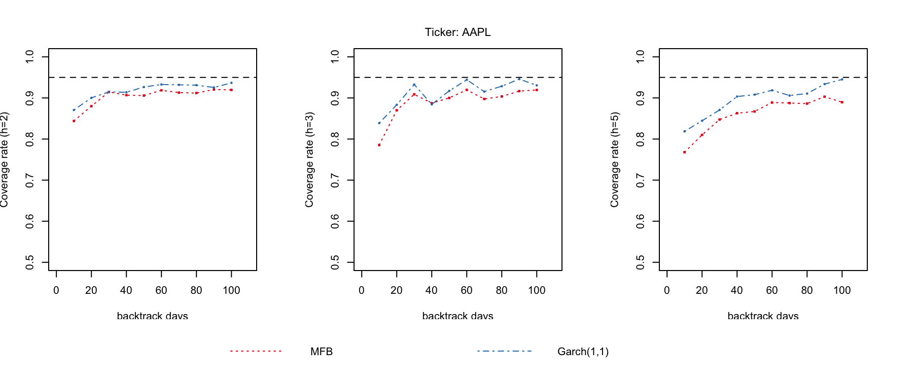
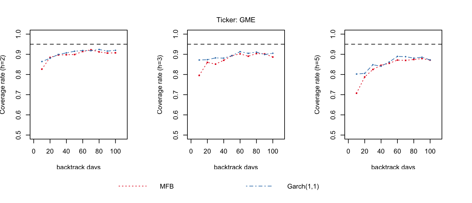
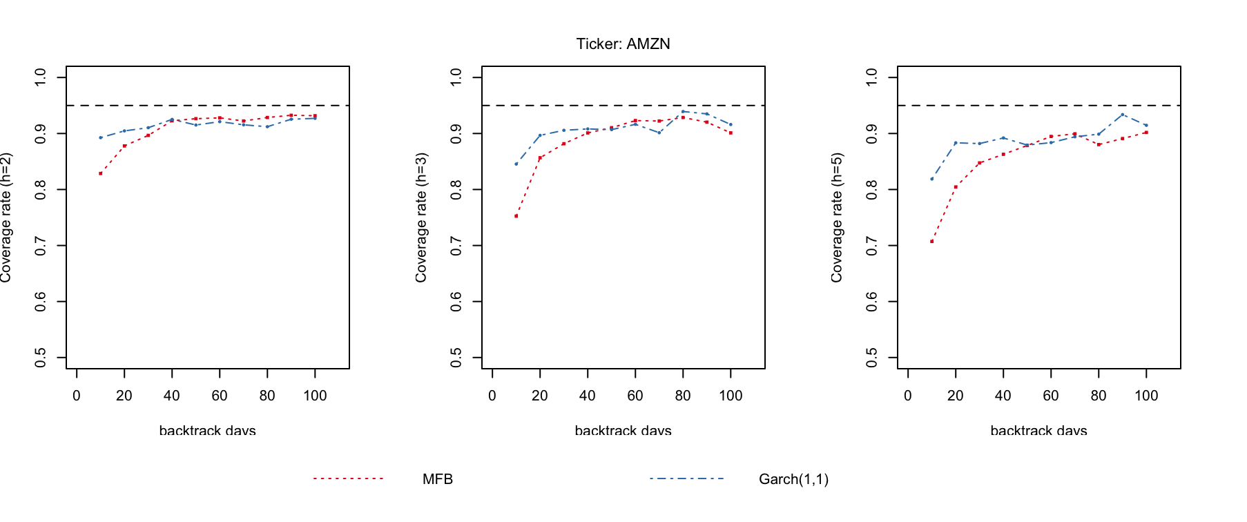
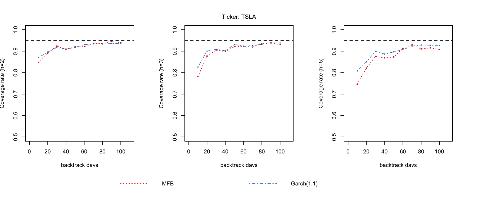
We can see that as the number of backtracking days increases, the empirical coverage also grows towards because of asymptotic validity. However, both methods still have under coverage issue, partially due to the fact that the stationarity assumption does not perfectly fit the stock market. We also observe that for and , the performance of the two methods are on par with each other. However, for the garch-based bootstrap has superior performance comparing with the MFB. This is due to the more efficient parameter searching scheme in garch fitting, whereas for the MFB, the process of parameter searching mostly relies on cross validation, which can be inefficient and suboptimal.
References
- Breuer and Major [1983] P. Breuer and P. Major. Central limit theorems for non-linear functionals of gaussian fields. Journal of Multivariate Analysis, 13(3):425–441, 1983.
- Chen and Politis [2019] J. Chen and D. N. Politis. Optimal multi-step-ahead prediction of arch/garch models and novas transformation. Econometrics, 7(3), 2019.
- Das and Politis [2020] S. Das and D. N. Politis. Predictive inference for locally stationary time series with an application to climate data. Journal of the American Statistical Association, 2020. To appear.
- Hull and White [1998] J. C. Hull and A. D. White. Value at risk when daily changes in market variables are not normally distributed. The Journal of Derivatives, 5(3):9–19, 1998.
- Jentsch and Politis [2015] C. Jentsch and D. N. Politis. Covariance matrix estimation and linear process bootstrap for multivariate time series of possibly increasing dimension. Ann. Statist., 43(3):1117–1140, 06 2015.
- McMurry and Politis [2010] T. L. McMurry and D. N. Politis. Banded and tapered estimates for autocovariance matrices and the linear process bootstrap. Journal of Time Series Analysis, 31(6):471–482, 2010.
- Patton [2013] A. Patton. Chapter 16 - copula methods for forecasting multivariate time series. In G. Elliott and A. Timmermann, editors, Handbook of Economic Forecasting, volume 2 of Handbook of Economic Forecasting, pages 899–960. Elsevier, 2013.
- Politis [2007] D. N. Politis. Model-free versus Model-based Volatility Prediction. Journal of Financial Econometrics, 5(3):358–359, 03 2007.
- Politis [2015] D. N. Politis. Model-Free Prediction and Regression: A Transformation-Based Approach to Inference. Springer, New York, 2015.
- Samorodnitsky and Taqqu [1994] G. Samorodnitsky and M. S. Taqqu. Stable Non-Gaussian Random Processes. Routledge, New York, 1994.
- Wang and Politis [2019] Y. Wang and D. N. Politis. Model-free bootstrap for a general class of stationary time series, 2019.
- Wilson and Ghahramani [2010] A. G. Wilson and Z. Ghahramani. Copula processes. In Advances in Neural Information Processing Systems(NIPS), volume 23. Curran Associates, Inc., 2010.
- Wolf and Wunderli [2015] M. Wolf and D. Wunderli. Bootstrap joint prediction regions. Journal of Time Series Analysis, 36(3):352–376, 2015.