Systematically Testing Singlet Models for Preprint: FERMILAB-PUB-21-012-T
Abstract
We comprehensively study all viable new-physics scenarios that resolve the muon anomaly with only Standard Model singlet particles coupled to muons via renormalizable interactions. Since such models are only viable in the MeV – TeV mass range and require sizable muon couplings, they predict abundant accelerator production through the same interaction that resolves the anomaly. We find that a combination of fixed-target (NA64, ), -factory (BABAR, Belle II), and collider (LHC, muon collider) searches can cover nearly all viable singlets scenarios, independently of their decay modes. In particular, future muon collider searches offer the only certain test of singlets above the GeV scale, covering all higher masses up to the TeV-scale unitarity limit for these models. Intriguingly, we find that muon colliders may yield better coverage for GeV-scale singlets compared to TeV-scale concepts, which has important implications for the starting center-of-mass energy of a staged muon collider program.
1 Introduction
The Fermilab Muon collaboration has recently released its first measurement of the muon’s anomalous magnetic moment Muong-2:2021vma; Muong-2:2021ojo; Muong-2:2021ovs; Muong-2:2021xzz. Their new results are consistent with previous Brookhaven measurements Muong-2:2006rrc, so the world average for now deviates from its Standard Model (SM) phenomenological prediction Aoyama:2020ynm; Aoyama:2012wk; Aoyama:2019ryr; Czarnecki:2002nt; Gnendiger:2013pva; Davier:2017zfy; Keshavarzi:2018mgv; Colangelo:2018mtw; Hoferichter:2019mqg; Davier:2019can; Keshavarzi:2019abf; Kurz:2014wya; Melnikov:2003xd; Masjuan:2017tvw; Colangelo:2017fiz; Hoferichter:2018kwz; Bijnens:2019ghy; Colangelo:2019uex; Pauk:2014rta; Danilkin:2016hnh; Jegerlehner:2017gek; Knecht:2018sci; Eichmann:2019bqf; Roig:2019reh; Colangelo:2014qya by
| (1) |
which yields a statistically significant discrepancy and may be the first laboratory evidence of physics beyond the SM (BSM).11 1 Lattice calculations of the Hadronic light-by-light contribution to Gerardin:2019vio; Blum:2019ugy; Chao:2021tvp as well as previous lattice calculations of the Hadronic Vacuum Polarization (HVP) FermilabLattice:2017wgj; Budapest-Marseille-Wuppertal:2017okr; RBC:2018dos; Giusti:2019xct; Shintani:2019wai; FermilabLattice:2019ugu; Gerardin:2019rua; Aubin:2019usy; Giusti:2019hkz are in agreement with the phenomenological values. However, a more recent calculation of the HVP from the BMW collaboration Borsanyi:2020mff implies a value of that is consistent with the measured value. This calculation might be in tension with the SM electroweak fit Passera:2008jk; Crivellin:2020zul; Keshavarzi:2020bfy, for which future lattice calculations and improved -ratio data will likely be needed to clarify this situation. If the anomaly is due to BSM states, their presence induces the effective operator
| (2) |
where and are the muon Weyl spinors, GeV is the Higgs vacuum expectation value (VEV), is a dimensionless coefficient and is a BSM mass scale. This effective operator generates a contribution to that can in principle resolve the anomaly by setting . If the BSM states are charged under the electroweak (EW) gauge group, there is a vast landscape of models that can resolve the anomaly (see Refs. Capdevilla:2020qel; Capdevilla:2021rwo; Athron:2021iuf for a review), hereafter referred to as electroweak (EW) models. Such models tend to have multiple free parameters and can, in principle, span a mass range for anywhere between 100 GeV100 TeV Capdevilla:2020qel; Capdevilla:2021rwo; Athron:2021iuf; Dermisek:2013gta; Freitas:2014pua; Queiroz:2014zfa; Calibbi:2018rzv; Dermisek:2021ajd; Arkani-Hamed:2021xlp; Dermisek:2021mhi.
However, if the BSM states that generate Eq. (2) are singlets under the SM gauge group (singlet models), the Higgs VEV and chirality flip in Eq. (2) must both arise from the muon mass, so Eq. (2) becomes proportional to ,
| (3) |
where is the mass of a SM singlet particle that has been integrated out to generate these operators. This feature greatly simplifies the model landscape down to two renormalizable interactions:
| (4) |
corresponding to BSM scalars () and vectors (), respectively, and greatly compresses the parameter space compared to EW models because of the muon mass suppression.22 2 Alternative possibilities involving pseudo-scalars or axial vectors contribute the wrong sign to and do not resolve the anomaly, and interactions whose leading contribution to involves two-loop diagrams are severely constrained – see Appendix A for a discussion.

In this paper, we systematically analyze all singlet models that resolve the anomaly and survey how numerous proposed experiments can cover much of the remaining viable parameter space. Every singlet model can be uniquely specified by a dimensionless coupling , a corresponding singlet mass , and a possible additional decay width of the singlet to other non-muonic particles. Thus, singlet models are generically more predictive than electroweak models and can be studied without specifying many model-dependent features (for instance, the particle spectra of supersymmetric models). However, because the scalar singlet interaction in Eq. (4) is not gauge-invariant under the SM, it must be UV-completed, and the extra particles required for this UV completion will play an important role in further restricting the parameter space of the scalar singlet model once constraints from e.g. electroweak precision observables are taken into account.
This paper is organized as follows. In Section 2 we summarize the landscape of singlet models and identify the allowed parameter space in each scenario, which is bounded from below by cosmology and from above by unitarity. In Sections 3, 4, and 5 we discuss future prospects for fixed target experiments, -factories, and collider experiments, respectively. We conclude in Section 6 with an outlook on the types of experiments needed to fill any remaining gaps in parameter space to conclusively test singlet explanations for . Our main results are summarized in Figure 3. The Appendices contain discussions of 2-loop models, searches for singlets with non-muonic visible decays, and UV completions of the scalar singlet models.
2 Singlet Models
Throughout this paper, Singlet Models refers to the family of models where one of the interactions in Eq. (4) generates in Eq. (1). In this section, we outline the general properties of these models and identify their viable parameter space for resolving the anomaly.
2.1 Vector Singlets
For a vector singlet with no axial couplings, the partial decay width to di-muons is
| (5) |
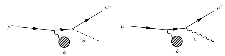
for . The vector contribution to from Fig. 1 (left) can be written
| (6) |
and the favored parameter space for resolving the anomaly is shown in the orange band of Fig. 2. In principle, there are many possible choices for abelian SM extensions that contain a vector-muon interaction. However, for anomaly-free U(1) gauge extensions to the SM, the favored parameter space for resolving is already excluded in most variants.
- •
Kinetically-mixed dark photon
The popular kinetically-mixed “dark photon” model features a new vector singlet corresponding to a secluded U(1) gauge group under which SM fermions carry no charges Pospelov:2008zw. In this scenario the muon-dark photon coupling is induced through kinetic mixing between dark and visible photons, so the dark photon couples to all charged fermions with equal strength. Consequently, this model is excluded as a solution to by a variety of -factory, beam dump, and rare meson decay searches – see Ilten:2018crw; Bauer:2018onh for a summary of constraints. This conclusion holds regardless of whether the dark photon decays visibly or invisibly.33 3 However, there is a limited parameter space for exotic decays that yield both visible and invisible particles via dark sector cascades in each decay event and may be tested with dedicated factory and fixed target searches Mohlabeng:2019vrz.Figure 2: Left: Parameter space for which one SM singlet scalar or vector particle resolves the anomaly. The thickness of each band represents the confidence interval and the vertical axis is the corresponding muon-singlet coupling from Eq. (4). The vertical shaded region represents the bound on light relativistic species present in equilibrium during big bang nucleosynthesis. The horizontal shaded region is the bound from partial wave unitarity. For a discussion of these bounds, see Section 2.3. Right: Minimum di-muon branching fraction for vector and scalar couplings that resolve the anomaly, from Eqs. (9) and (15). - •
Anomaly-free U(1) extensions
Minimal abelian extensions to the SM promote an anomaly-free linear combination of baryon , lepton , and lepton flavor quantum numbers, where , to a gauge symmetry. Some examples include , , . Since nearly all of these options include some coupling to first-generation SM fermions, they are subject to the same constraints that apply to the dark photon and are, therefore, also excluded He:1990pn; Dror:2017nsg; Ballett:2019xoj (unless new fields are introduced Allanach:2015gkd; Raby:2017igl; Kawamura:2019rth; Bodas:2021fsy; Mondal:2021vou; Greljo:2021xmg; Lee:2021gnw). A well known exception is gauged Altmannshofer:2014pba; Escudero:2019gzq; Krnjaic:2019rsv; Holst:2021lzm, which has no tree-level couplings to first-generation particles and evades many of the bounds that arise from couplings to protons and electrons. This model is viable for vector masses in the 15 – 210 MeV range Escudero:2019gzq in which decays exclusively to neutrinos and can be tested with low-energy fixed-target experiments – see Sec. 3 for more details.In the case of the most general extension for including right-handed neutrinos (needed for anomaly cancellation) one can have a vast family of models Greljo:2021npi. These can be classified as dark photon-like or -like in case they include (former) or not (latter) interactions with first generation leptons. Most of these models are either excluded or highly constrained Greljo:2021npi.
- •
Anomalous U(1) extensions
Since most bounds on anomaly-free U(1) models involve constraints on their non-muonic interactions, in principle it is possible to open up parameter space by coupling the vector only to muons. However, such an approach introduces interactions that grow with energy via non-decoupling triangle diagrams that amplify otherwise rare SM processes Dror:2017nsg; Kahn:2016vjr; Dror:2017ehi. While such models have not been studied exhaustively in the context of explaining , it is expected that they would be strongly constrained by existing bounds (e.g. rare meson decays involving muon final states). We note that a fully unitary theory with anomalous interactions at low energies must ultimately invoke additional SM charged states to cancel triangle diagrams at some scale; however, there is considerable model dependence in how this is achieved.
For the remainder of this paper, we will take an agnostic approach towards the models that realize the vector-muon coupling, while noting that specific realizations of vector singlets might have additional bounds beyond those that we present. Taking into account only the irreducible coupling to muons which generates , we will present a phenomenological treatment that studies only di-muon decays or invisible decays,
| (7) | |||||
| (8) |
where also allows for a long-lived that effectively gives rise to missing energy signatures. For in this agnostic approach, the total width is bounded by unitarity at Schwartz:2014sze. Saturating this maximum width, even if the dominant branching fraction is into other channels (visible or invisible), the minimum vector branching fraction to di-muons is
| (9) |
where we have used Eq. (5) in the limit and expressed Eq. (6) in terms of the central value in Eq. (1); this minimum value applies to any vector singlet that resolves the anomaly. In Fig. 2 (right panel) we show the minimum branching fraction as a function of singlet mass.
As an example of how this general analysis becomes constrained in the context of particular models, if is the gauge boson of an anomaly-free group involving , then the only viable parameter space is for with predominantly invisible decays, since is excluded by the irreducible visible decay channel. Other channels due to, for example, a small kinetic mixing between and the photon, are strongly suppressed.
2.2 Scalar Singlets
For scalar singlets, the partial decay width to di-muons is
| (10) |
for , and the corresponding contribution to from Fig. 1 (right) can be written
| (11) |
The favored parameter space for resolving the anomaly is shown in the green band of Fig. 2. This contribution is comparable to the corresponding expression for vector singlets in Eq. (6).
Unlike in the vector case, the scalar Yukawa interaction in Eq. (4) is not gauge-invariant under SU(2) U(1)Y and must arise from a higher-dimension operator. In principle, this could be avoided if mass-mixes with the SM Higgs. However, the SM Higgs-muon Yukawa coupling is , so from Fig. 2, such a contribution is too small for all but the lightest masses, even before taking into account strong suppression from the singlet mass or its tiny mixing angle with the Higgs Krnjaic:2015mbs. Thus, the lowest-dimension operator that can generate a flavor-specific coupling to muons is
| (12) |
where is the second-generation lepton doublet and is a BSM mass scale generated by heavier particles that are integrated out to generate the singlet-muon Yukawa coupling after electroweak symmetry breaking.
We defer a detailed discussion of UV completions for the scalar singlet scenarios to Section 5.2 and Appendix C. Here we only point out that since scalar Yukawa interactions are not constrained by anomaly cancellation requirements, the flavor structure of these interactions is only constrained by experimental considerations:
- •
Mass Proportional Couplings:
As noted above, cannot mass-mix with the SM Higgs because the muon Yukawa is too small to explain , but a larger muon coupling can be achieved if is part of a two-Higgs doublet model with leptophilic couplings. In such a model, the scalar couplings are proportional to charged lepton masses and can be larger than their nominal SM values (see Batell:2016ove; Chen:2017awl for an example). However, the parameter space for resolving the anomaly within this model has been excluded by the BABAR experiment in a null search for BSM events BaBar:2020jma. - •
Flavor Specific Couplings:
The interaction in Eq. (12) can also arise by coupling the singlet to new electroweak-charged fermions that mix with the muon, followed by integrating them out at some scale . In principle, such an approach allows any flavor structure (subject to empirical constraints) and many options have been considered in the literature Chen:2015vqy; Batell:2017kty; Hiller:2019mou; Egana-Ugrinovic:2019wzj; Liu:2020qgx; Hiller:2020fbu; Bissmann:2020lge; Batell:2021xsi.
Thus, for the remainder of this paper, we will not assume any particular flavor structure in the couplings. For light scalars below the di-muon threshold, we will consider
| (13) |
As before, represents invisible decays or a long-lived . Note that for singlet scalars, the di-photon coupling arises at one-loop through the coupling to muons, which is required for .44 4 Of course, this contribution can be tuned against an additional higher-dimension term present in the Lagrangian, but this term would require its own UV completion, and fine-tuning the photon coupling away entirely requires an exquisite coincidence of scales. As we will see in Sec. 3.1, the decay length assuming only the channel is macroscopic, such that it may manifest as missing energy in a collider experiment but be visible at a beam-dump experiment. Note also that the channel is forbidden for vectors by the Landau-Yang theorem. Since is not required by and depends on the flavor structure of the model, in our model-agnostic treatment we will not consider it in detail in this work, but we briefly comment on this channel in Appendix B. For scalars above the di-muon threshold, we will consider the irreducible decay channel
| (14) |
As in the vector case discussed above, the minimum muon couplings required for and the unitarity upper limit on the singlet’s total width imply a minimum di-muon branching fraction independently of other decay channels
| (15) |
where we have used Eq. (10) in the limit and followed the same logic that leads to Eq. (9) in the vector case. In Fig. 2 (right panel), we show the minimum branching fraction as a function of singlet mass.
2.3 Viable Mass Range
Although the couplings required to explain for light singlets are feeble from a collider perspective, they nonetheless suffice to thermalize these new states with the SM radiation bath in the early universe, provided the initial temperature exceeds a given choice of singlet mass. For light singlets (), the early universe production and annihilation rates scales as , where is the temperature of the radiation bath. Comparing this rate to Hubble expansion implies thermalization for temperatures
| (16) |
where is the number of relativistic species in the bath and GeV is the Planck mass. Thus, for singlet masses below the MeV scale with couplings that resolve the anomaly in Fig. 2 (left panel), there will be a thermal number density of singlets in the early universe at temperatures , which increases the expansion rate during Big Bang Nucleosynthesis (BBN) and spoils the successful SM prediction of light element yields. Avoiding the BBN bound requires Escudero:2019gzq; Krnjaic:2019dzc
| (17) |
which are represented in the shaded regions labeled “cosmology” in Figs. 2 and 3.
For singlets above the muon mass, the BSM contribution to scales as so, in principle, any choice of mass can resolve the anomaly. However, for sufficiently large couplings, singlet interactions violate partial wave unitarity. As shown in Capdevilla:2021rwo, imposing tree-level unitarity constraints on muonic Bhabha scattering through an - or -channel yields and . This implies an upper bound of and , or a UV completion involving additional states at the same mass scale as the singlet itself. The combination of cosmology and unitarity constraints provides a robust two-sided boundary to the viable mass range for singlet solutions to :
| (18) |
In Fig. 3, we show the viable parameter space for both visibly- and invisibly-decaying and , along with constraints and projections from fixed-target experiments, -factories, and colliders, which we discuss in detail in the following sections.
3 Fixed Targets
Fixed-target experiments are a promising strategy to search for new light ( GeV) weakly-coupled SM singlet particles in a variety of contexts Altmannshofer:2014pba; Chen:2017awl; Kahn:2018cqs; Battaglieri:2017aum; Izaguirre:2013uxa; Berlin:2018bsc; BDX:2019afh; Berlin:2018pwi; NA64:2017vtt; Proceedings:2012ulb; Blumlein:2011mv; Celentano:2014wya; Gninenko:2014pea; Gninenko:2019qiv; Kahn:2012br; Balewski:2014pxa; Batell:2014mga; Izaguirre:2014bca, including the idea of using the ATLAS calorimeters as a fixed-target Galon:2019owl. As discussed in Sec. 2, viable models for with light singlets require muon-philic interactions, but most fixed-target experiments involve beams of electrons or protons and are, therefore, insensitive to the remaining parameter space that resolves the anomaly. However, several new muon-beam fixed-target experiments have recently been proposed to address this shortcoming by exploiting singlet production in muon-nucleus scattering, see Fig. 4.
3.1 Beam Dump Searches for
In a beam dump experiment, a high-intensity muon beam impinges on a large, dense target which is surrounded by shielding material to block SM particles. If a long-lived, visibly-decaying singlet is produced in the dump, it can travel unimpeded through the shielding and decay to visible SM particles in a downstream detector.
Such a setup can cover nearly all of the remaining parameter space for scalar singlets with that decay via , induced at one-loop through the minimal scalar-muon Yukawa coupling required to address the anomaly Chen:2017awl:
| (19) |
where is an order-one number and in the second expression the muon has been integrated out. If the - Yukawa coupling is the only contribution to this operator, then for that resolve anomaly, the decay length is Chen:2017awl
| (20) |
where is the energy of the particle and the fiducial values for and are chosen to match the favored parameter space in Fig. 2 (left panel).
In the top-right plot of Fig. 3 we show the projections from Ref. Chen:2017awl for a proposed beam dump search for long lived particles with a 3 GeV beam and muons on target, assuming only the minimal muon-induced coupling to di-photons (Model B from Ref. Chen:2017awl). However, note that if other model-dependent decay processes are introduced, the singlet might not be a long-lived particle and this search strategy would lose sensitivity. Similar sensitivity could be achieved for the channel if the singlet-electron coupling is chosen to reproduce the same decay length as in Eq. (20), but unlike the minimal muon-induced di-photon decay, this displacement scale does not automatically follow from the same coupling that resolves the anomaly (also see Appendix B for further discussion).
3.2 Missing Momentum Searches for
The proposed NA64 Gninenko:2014pea; Gninenko:2019qiv and Kahn:2018cqs experiments aim to test the remaining parameter space for invisibly-decaying singlet particles. In these experiments, a muon beam of moderate intensity impinges on an active target, which monitors the beam energy as it passes through. Signal events are those where the outgoing muon energy is reduced by and no other SM particles are observed in downstream veto detectors; the limiting factor for the luminosity is the requirement to only have a single muon per bunch to mitigate pileup. In Figure 3, we show the NA64 and projections for and muons on target, respectively; these reference values match the ultimate reach projections from Refs. Gninenko:2014pea and Kahn:2018cqs, where Ref. Gninenko:2014pea only considered invisibly-decaying vectors. Note that these projections cover the remaining parameter space that resolves the discrepancy within the anomaly-free gauge extension discussed in Sec. 2.1, where there is an order-1 invisible branching fraction to neutrinos for . Preliminary data is expected from NA64 Sieber:2021fue in the very near future.
4 -Factories
We now discuss -factory searches for singlets decaying to muons. Singlet models generate new contributions to events from processes in which the singlet or is radiated from a final-state muon line and decays via , as depicted in Fig. 5. This search strategy can test the favored parameter space for light singlets with appreciable branching fractions to di-muons, but other search strategies are necessary for invisibly-decaying singlets. We briefly comment on other visible final-state searches at -factories in Appendix B.
The BABAR collaboration has performed a search for muon-philic vectors with gauge interactions and excluded the favored parameter space for masses between and 10 GeV with 514 fb-1 of data BaBar:2016sci. Since an gauge boson in this mass range can decay to muons, taus, and their corresponding neutrino flavors, in Fig. 3 (left panel) we rescale their limit for our vector for which BR; for models in which has a smaller branching fraction, the limit on gets weaker by a factor of .
In the right panel of Fig. 3, we reinterpret the BABAR limits from Ref. BaBar:2016sci in the context of our scalar singlet model.55 5 Similar BABAR limits on muon-philic scalars were also calculated in Refs. Chen:2017awl and Krnjaic:2019rsv. Unlike Ref. Krnjaic:2019rsv, which approximated the BABAR limit with a smooth curve, we apply the full mass dependence of the limit from the reported bounds from BaBar:2016sci, which results in a more jagged curve in our Fig. 3 (right). Also in contrast to Ref. Krnjaic:2019rsv, we apply the full geometric acceptance to the rescaling. Having already obtained the limit for vectors , we can obtain the limit for scalars by applying the rescaling
| (21) |
where is the singlet production cross section, is the geometric acceptance, and each of the quantities here is mass-dependent. To obtain the necessary quantities for this rescaling, we simulated production events using MadGraph5 Alwall:2014hca; Alwall:2011uj which enable us to extract the cross sections and geometric acceptances assuming angular coverage in the BABAR lab frame, where is the polar angle of the final-state muon defined with respect to the incident electron beamline. We have also have verified that our simulated events adequately reproduce the limits reported in Ref. BaBar:2016sci when adapted to that scenario.
In both panels of Fig. 3 we also show future projections for a 4 search at Belle II with 50 ab-1 of luminosity. Here we assume that the BABAR background model and statistical uncertainties from Ref. BaBar:2016sci can be adapted to the Belle II experimental setup with a rescaled luminosity. To place a limit on the singlet couplings, we demand that the signal in each bin of di-muon reduced mass not exceed the expected SM background by more than 2, where is the reduced mass of an opposite state di-muon pair in the final state. A more rigorous, Belle II-specific systematic analysis is beyond the scope of this paper, but would be interesting for future work. Since the Belle II luminosity improves upon the BABAR data set by a factor of , this search alone will cover all remaining scalar singlets with mass between and 10 GeV unless their branching fraction is to di-muons is less than 1%.
5 Collider Searches
We now discuss direct singlet searches at the LHC in the 3- and 4-muon final states, as well as inclusive singlet searches at future muon colliders. Since LHC searches have limited mass reach for scalars, it is important to take electroweak precision constraints from all possible types of UV completions for singlet scalar models into account, which sets a more restrictive upper mass limit than unitarity alone. Even so, we find that future muon colliders are required to exhaustively probe singlet explanations of the anomaly.
5.1 Singlet Production at the LHC
In order to produce or at a hadron collider, one needs to produce either one or two muons via charged or neutral Drell-Yan processes and then let one of the muons radiate a singlet. These processes are depicted in Fig. 6. Because the singlets can decay promptly back to a muon pair, the overall reactions look like three- and four-muon production, respectively. Backgrounds for these reactions include similar processes to those in Fig. 6, replacing the singlets by a boson that further decays into a pair of muons, as well as production where the vector bosons decay leptonically. These irreducible backgrounds combined can be sizeable compared to the signals, but with proper cuts on the invariant mass of opposite-charge di-muon pairs, one can isolate the signals with great sensitivity in the case where the singlets decay 100% to muons.
For our analysis, we implemented the Lagrangian Eq. (4) in FeynRules2 Christensen:2008py; Alloul:2013bka and generated charged and neutral Drell-Yan events with MadGraph5 Alwall:2014hca; Alwall:2011uj. (For this clean muon signal, detector resolution and efficiency effects play a subdominant role and can be neglected in our estimates.) The cross sections for three- (left) and four-muon (right) production are presented in Fig. 7 where the SM background is shown in dashed gray and the vector and scalar singlets are shown in orange and green, respectively. These cross sections were obtained using the same loose cuts implemented in the four-lepton search by ATLAS in ATLAS:2021kog: GeV (leading muon), GeV (sub-leading muon), GeV (the other muons), , , and GeV, where the small angular acceptance is required to allow topologies where a boosted particle decays into a pair of muons, and the cut in the invariant mass of any pair of opposite-sign muons is imposed to exclude leptons from quarkonia. These cross sections show that even without further cuts, the high-luminosity LHC (HL-LHC) should be able to probe singlet scalar masses up to , but as we show below, the mass reach can be significantly increased by making use of the resonant nature of on-shell singlet production.
Note that in Fig. 7, the vector and the scalar production cross sections differ by about two orders of magnitude. This is for two reasons. First, the coupling fixed by is larger for vector singlets than for scalars by about a factor of three in the region above GeV as shown in Fig. 2 (left). Second, due to the chiral flip at the scalar vertex in Eq. (4), the overall scalar production is a helicity-1 to a helicity-0 transition, so it is -wave suppressed. This does not happen in vector models where an -wave transition is possible, because the vector does not flip the chirality of the fermion lines. Also note that the charged Drell-Yan process () has a larger cross section than the neutral one (). This is because couplings to fermions are larger than couplings, and because the process includes two channels () whereas includes only one channel () and an extra suppression by statistical factors for identical particles in the final states.
Amongst recent LHC searches, the most relevant ones for this signal are two analyses conducted by ATLAS searching for new physics in and final states ATLAS:2021kog; ATLAS:2021wob, as well as a search for gauge bosons by CMS CMS:2018yxg. The CMS search can be applied almost verbatim to our singlet vector scenario. Assuming the acceptances do not change significantly, we can also recast this search for the singlet scalar using the ratio between the vector and scalar singlet cross sections in Figure 7. The resulting limits are shown in Figure 3 and already exclude singlet scalar (vector) explanations of the anomaly in the mass range (), if these singlets decay exclusively to muons.
The mass reach can be significantly extended by dropping the requirement of an intermediate on-shell boson, and also considering final states. This means that recent multi-muon ATLAS analyses ATLAS:2021kog; ATLAS:2021wob have great exclusion power for these singlet scenarios. Unfortunately, these analyses do not explicitly look for an intermediate di-muon resonance. However, if the di-muon invariant mass distribution we describe below were made public for this or future such analyses, then these searches could supply the best limits on singlet scenarios that resolve the anomaly.
To demonstrate this, we derive sensitivity projections by considering the combined distribution of invariant masses of all possible opposite-sign di-muon pairs in each event. Because there are multiple muons in the final states, the combinatorial background tends to spread the invariant mass spectrum over a wide range of values. Even so, the singlet- and -resonances remain clearly visible in the signal and background. For each singlet mass, we define a signal region in this combined distribution that is centered on . The signal region has a variable width, ranging from 10 GeV for the lowest up to 30% of the singlet mass for larger values of .66 6 This is highly conservative for narrow-width singlets. For singlets with decay width near the unitarity bound, our signal region as defined will not cover the full resonance width, but as our results indicate, for singlets with large invisible width, direct LHC searches for the muon final state are completely ineffective anyway.
Fig. 8 shows the LHC luminosity required using this strategy to exclude singlet scenarios that resolve the anomaly for masses above 5 GeV. This corresponds to a combined analysis of bump hunts in both charged and neutral Drell-Yan events, which we refer to from here on as a search. The events dominate the constraints for low singlet masses, whereas events dominate for large masses. The solid curve corresponds to the optimistic scenario where the singlets decay with a 100% branching ratio to muons, while the dashed curve corresponds to the minimum irreducible branching fraction to muons as shown in Fig. 2 (right).
In the optimistic scenario, one can see that searches at the LHC can probe singlet vector masses up to 700 GeV with current luminosity , whereas with the expected luminosity at HL-LHC the search could probe the entire parameter space up to the perturbativity limit at about 1 TeV. As discussed above, the signal cross section for scalars is much smaller than for vectors for a given singlet mass. For this reason the reach of the search is not as promising in the case of scalar singlets. With current (future) luminosity, the LHC could probe masses up to 50 (60) GeV. If the singlets only have the minimum irreducible branching ratio to muons, direct searches at the LHC have almost no power to probe this scenario. Even so, it is clear that this strategy greatly increases the mass reach compared to a search that is restricted to exotic decays. Figure 3 shows these HL-LHC projections as bounds on .
5.2 Electroweak Precision Constraints and Singlet Scalar UV Completions
As we can see from Fig. 8, singlet scalars can only be directly probed with searches at the HL-LHC if . It seems very difficult to directly probe heavier scalars coupling only to muons at a proton collider. Fortunately, we can exploit the fact that the scalar singlet model must have a UV completion featuring new electroweak charged states.
As discussed in Section 2.2, the scalar Yukawa interaction in Eq. (4) is not gauge-invariant and must arise from the dimension-5 operator
| (22) |
where is some BSM mass scale. We will assume that this operator is generated by tree-level exchange of some heavy mediator; if this interaction is somehow generated at higher loop level, the resulting electroweak states will be much lighter, resulting in even tighter constraints. There are only three possible types of diagrams that can generate this operator at tree-level, shown in Figure 9: exchange of a fermion mediator that is an singlet, a doublet fermion mediator, or a doublet scalar mediator. The top two diagrams to the right correspond to what we call fermion UV completions and the bottom-right diagram is the scalar UV completion for the singlet scalar model. After electroweak symmetry breaking, the former class features heavy fermions that mix with the muon, whereas the latter features a heavy scalar doublet that mixes with the scalar singlet .

It is easy to understand why electroweak precision tests (EWPT) ParticleDataGroup:2020ssz can constrain these UV completions. If the singlet accounts for the anomaly via an effective coupling to the muon as in Figure 2, then heavier singlets require lower masses and/or larger couplings for the new mediator states. To derive indirect constraints on scalar singlet scenarios, we make the minimal assumption that the scenario is UV-completed by a single one of these three mediator types.
The main EWPT we focus on in our analysis is the modified lepton universality ratio
| (23) |
In the SM, this ratio is close to unity except for small phase space differences and small loop corrections. Under the assumption that the singlet scalar resolves the anomaly, both scalar and fermion UV completions generate significant vertex corrections that can be probed by LEP measurements ParticleDataGroup:2020ssz. For scalar UV completions, the presence of additional scalars with electroweak charges also gives additional contributions to production at the LHC. The details of this analysis are provided in Appendix C. The important point is that we always consider the minimal size of allowed by adjusting the various mediator couplings within the bounds set by unitarity, and that the simple singlet scalar model of Eq. (4) is a good IR effective theory in the non-excluded regions of parameter space. Our main results are the following:
- •
Fermion UV completions of the singlet scalar violate EWPT for .
- •
Scalar UV completions of the singlet scalar violate EWPT for .
- •
If the singlet scalar only couples to the muons, then additional contributions to production at the LHC, together with EWPT, exclude .
Since these constraints were derived by directly relating the required size of the dimension-5 operator Eq. (12) (to generate ) to the corresponding minimal vertex correction, it is unlikely that these constraints would be greatly affected by considering more non-minimal UV completions, since additional couplings generally lead to additional observable effects unless deliberate cancellations are enforced. Therefore, it appears that with current LEP constraints, singlet scalar scenarios cannot be consistent with masses above roughly 615 GeV, which has implications for future colliders that could aim to directly produce these singlets. We indicate this upper mass bound as the vertical dashed gray line in Figure 3.
5.3 Future Muon Colliders
Muon colliders have recently attracted considerable interest as successor machines to the LHC Alexahin:2018svu; Buttazzo:2018qqp; Boscolo:2018ytm; Neuffer:2018yof; DiLuzio:2018jwd; Delahaye:2019omf; Shiltsev:2019rfl; Costantini:2020stv; Han:2020uid; Han:2020pif; Han:2020uak; Bandyopadhyay:2020otm; Buttazzo:2020uzc; Huang:2021nkl; Liu:2021jyc; Chen:2021rnl; Han:2021udl; Collamati:20216A; Capdevilla:2021fmj; Huang:2021biu; Han:2021kes; Bottaro:2021srh; AlAli:2021let; Chiesa:2020awd; Long:2020wfp; Asadi:2021gah; Franceschini:2021aqd; Collamati:2021rbr; Sen:2021fha; Bandyopadhyay:2021pld; Qian:2021ihf; Chiesa:2021qpr; Liu:2021akf; Zaza:2021bj; Mastrapasqua:2021uvs; Zaza:2021nnq; Ruiz:2021tdt; Casarsa:2021rud. Representative muon colliders concepts at the energy frontier may feature multi-TeV scale center-of-mass energies and luminosities of order . Such facilities would be ideal laboratories for studying heavy, muon-philic interactions that cannot be probed robustly with existing proton or electron collider concepts Capdevilla:2021rwo. Indeed, it has been shown that such machines can perform model-independent tests of the anomaly via muonic Bhabha scattering Capdevilla:2021rwo and the channel Buttazzo:2020ibd; Yin:2020afe.
We have also shown in previous work that heavy singlets responsible for the anomaly can be directly tested through production independently of how the singlets decay Capdevilla:2021rwo. Since 2-body particle production yields back-to-back final-state recoils, this strategy triggers on events where the final-state photon is the only object in a detector hemisphere surrounding its momentum vector. Due to the large couplings required for heavy singlets (see Fig. 2), such production events can exceed the SM prediction for hemispherically-isolated single photons. Furthermore, since the observable is the isolated photon, the sensitivity of this strategy is independent of how the singlet decays as it recoils away from the photon. In Fig. 3 we show muon collider projections for singlet sensitivity assuming a 215 GeV (3 TeV) center-of-mass energy and 0.4 ab-1 (1 ab-1) of integrated luminosity as purple solid (dashed) curves. For the 215 GeV muon collider, singlets below are probed via direct production, while heavier singlets are probed through their virtual contributions to muonic Bhabha scattering (). At a 3 TeV muon collider, direct production is always more sensitive as long as the singlet can be produced on-shell, so the analogous Bhabha projections do not contribute to the exclusion curve we show.
6 Conclusions
In this paper we have systematically investigated solutions to in which a SM singlet generates the dominant contribution to the observed discrepancy via renormalizable interactions with muons. There are only two such classes of models, involving a singlet scalar or a vector , and both are highly restricted by general principles: scalars by the requirement of UV completion, and vectors by anomaly cancellation or non-decoupling triangle diagrams. Using only robust arguments from cosmology and unitarity, we constrain the viable mass range for singlets to lie between a few MeV and a few TeV Capdevilla:2020qel; Capdevilla:2021rwo. We have then surveyed a program of existing and future experiments to cover this parameter space, illustrated in Figure 3 and summarized here:
- •
Model-Independent Probes:
A future 215 GeV muon collider could cover the entire favored region above for vectors and about 1 GeV for scalars. A 3 TeV muon collider is less sensitive to light singlets, excluding all favored masses above about 1 GeV for vectors and 10 GeV for scalars. Notably, this is independent of how the singlet decays, as it only relies on the photon kinematics in events Capdevilla:2021rwo, or singlet contributions to Bhabha scattering. - •
Di-muon Decays:
If the singlet decays predominantly to di-muons (when kinematically allowed), the parameter space can be probed with a combination of -factory and high-energy collider searches. Current BABAR and LHC data, together with future Belle II and HL-LHC searches, can cover nearly the entire parameter space for vectors above ; scalar singlets will be robustly covered for masses between and . - •
Invisible Decays:
Missing energy/momentum experiments (including NA64, which will be taking preliminary data imminently) will cover the entire region below , for both scalars and vectors which decay invisibly on the scale of the experiment, and have additional reach into the GeV scale if the dominant decay is invisible, as is true for viable anomaly-free vector models such as an gauge boson. - •
Other Visible Decays:
The only remaining gap in the coverage presented here involves prompt visible decays to , and (or other visible exotics) for singlets in the MeV–10 GeV mass window; higher masses will be robustly covered with muon colliders, and displaced decays will be covered by missing-energy/momentum experiments at which long-lived particles yield missing energy. However, it is generically difficult to engineer prompt and visible decays for singlets that resolve in this mass range. All anomaly-free vector models with visible decays in this range have already been ruled out Bauer:2018onh, and anomalous vectors are likely subject to severe constraints from non-decoupling triangle diagrams. Scalar singlets can be viable, but the electron coupling is generically required to be smaller than the muon coupling, which would yield macroscopic decay lengths for much of the allowed mass range. Similarly, long decay lengths are expected if the scalar decays through the minimal di-photon coupling induced by integrating out the muon Chen:2017awl. We leave a more detailed study of this remaining parameter space with non-muonic decay channels for future work.
Thus, a broad program of energy and intensity frontier probes can robustly cover all the currently viable parameter space with only a few narrow exceptions.
We have also studied how the singlet scalar model may be UV completed, and there are just three classes of possibilities if the singlet-muon coupling is generated by tree-level exchange of heavy mediators. Electroweak precision measurements then suggest that the singlet scalar mass has to be less than about 600 GeV, a factor of five lower than the upper bound provided by naive unitarity arguments alone.
Our analyses show that even without a muon collider, the parameter space of singlets that solve the anomaly can be significantly probed by beam dumps, -factories, and HL-LHC searches. However, this leaves large gaps in coverage. For the optimistic scenario where the new singlet decays entirely to muons, scalars above 60 GeV are inaccessible. In the pessimistic scenario where the singlet only has the irreducible minimum branching ratio to muons required by unitarity, vectors between are inaccessible, while scalars represent something of a nightmare scenario, apparently impossible to see above with this suite of experimental probes.
On the other hand, it is clear that a muon collider is required to probe singlet scalar solutions to the anomaly. They are straightforward to UV complete with masses much larger than the HL-LHC reach, and it is similarly easy to imagine scenarios where they have other decays that hide them from muon searches. Furthermore, probing singlet solutions particularly motivates a staggered approach in center-of-mass energy for the muon collider program. A 3 TeV machine is obviously preferred to push the boundaries of the energy frontier, as well as to start probing solutions to that involve dominant contributions by new electroweak charged states Capdevilla:2021rwo. However, such a high-energy machine actually has more difficulty discovering light singlet scalars below 10 GeV, while direct production at a 215 GeV muon collider is sensitive down to the upper mass limit of proposed muon fixed-target experiments.
It is interesting to consider whether other experimental probes could fill the gap up to scalar masses of 10 GeV, so that no gap in coverage remains if only a multi-TeV muon collider were built. For both the scalar and the vector, the limited number of visible final states available in this narrow mass range should allow a complete enumeration of all of the possible visible and invisible decays for total widths approaching the unitarity limit. The outcome of such a study could have major implications for the future muon collider program by setting the minimum mass scale of new physics that such a high-energy machine would have to probe in order to leave no gaps in coverage. We leave this for future investigation.
The anomaly is quite possibly our best hint of new BSM physics in the laboratory. Our work highlights the need for muon colliders to comprehensively probe the new physics that must exist if the anomaly is real, from very high masses Capdevilla:2020qel; Capdevilla:2021rwo all the way down to the GeV scale. No other kind of experiment has such a wide dynamic range in energy and precision, and if SM explanations of the anomaly are ultimately excluded, a comprehensive muon collider program would be well motivated as a top priority for the international particle physics community.
Acknowledgements: We thank Nikita Blinov, Brian Shuve, Nathaniel Craig, and Kohsaku Tobioka for helpful conversations. The research of RC and DC was supported in part by a Discovery Grant from the Natural Sciences and Engineering Research Council of Canada, the Canada Research Chair program, the Alfred P. Sloan Foundation, and the Ontario Early Researcher Award. The work of RC was supported in part by the Perimeter Institute for Theoretical Physics (PI). Research at PI is supported in part by the Government of Canada through the Department of Innovation, Science and Economic Development Canada and by the Province of Ontario through the Ministry of Colleges and Universities. The work of YK was supported in part by US Department of Energy grant DE-SC0015655. This manuscript has been authored by Fermi Research Alliance, LLC under Contract No. DE-AC02-07CH11359 with the U.S. Department of Energy, Office of High Energy Physics.
Appendix A Appendix: Two-Loop Models
Throughout this paper, we have studied singlet particles that couple linearly to muon currents and resolve the anomaly at one loop through the Feynman diagrams shown in Fig. 1. However, it is logically possible that the leading contribution to involves two-loop diagrams instead. In this appendix we assess the feasibility of two representative two-loop scenarios.77 7 We thank Nathaniel Craig for posing this challenge.
A.1 Bilinear Scalar Couplings
In principle, a quadratic (or higher polynomial) scalar coupling could yield appreciable contributions to involving two-loop diagrams with no corresponding one-loop contributions. By SM gauge invariance, the lowest-dimension operator that yields a two-loop correction to involves a scalar with the interaction
| (24) |
where is a mass scale that arises from integrating out particles charged under SU(2) U(1)Y and we assume that the simpler Yukawa coupling is negligibly suppressed or forbidden due to a or other symmetry under which the is charged.
By naive dimensional analysis, the contribution to from the interaction in Eq. (24) is estimated to be
| (25) |
where the prefactor arises from the two-loop phase space and we demand GeV to avoid model-independent LEP bounds on new electroweak charged particles Egana-Ugrinovic:2018roi while maximizing their contribution to . Furthermore, this correction to saturates to a fixed value for , so the normalization in Eq. (25) represents the maximum contribution to the anomaly due to this interaction. Despite these extremal choices, the magnitude of the effect in Eq. (25) appears barely large enough to account for the necessary from Eq. (1) even if is sizeable, but is sufficiently close that a more careful calculation would be needed before fully excluding this possibility.
However, the interaction in Eq. (24) assumes that the two-loop interaction arises from integrating out a single particle with a coupling-to-mass ratio of order , without introducing any intermediate steps. In practice, resolving this higher-dimension operator with renormalizable and gauge-invariant interactions at energies above the scale is more challenging and further suppresses the BSM contribution to , effectively resulting in . Indeed, the only single-particle UV completion of Eq. (24) involves coupling to the Higgs doublet and integrating out the Higgs boson after EWSB to obtain
| (26) |
where GeV is the Higgs mass, is the SM muon Yukawa coupling, and is a dimensionless parameter. Here and , and for any unitary choice of , the contribution of Eq. (25) is much too small to explain the anomaly.
Avoiding this Yukawa suppression requires adding additional SM charged states that couple to both the muon and the Higgs (for example, chiral fermions which mass-mix with the muon). These states must also couple to the SM-singlet operator , which is dimension-2 and cannot couple to a dimension-3 fermion bilinear with a renormalizable interaction, so an additional scalar must also be added and then integrated out to generate at low energies. However, if this additional scalar couples linearly to the bilinear, it introduces quantitatively larger one-loop contributions to , which invalidates our motivation; if its coupling to this bilinear arises from some other interaction, even more fields must be added to the theory and integrated out. Furthermore, despite these difficulties, the net effect of performing all these steps must still yield in Eq. (24), which seems implausible. While we have not presented a rigorous theorem to eliminate such a possibility, even if it were possible to generate a large prefactor and suppress all one-loop corrections to , its contribution would still be too small based on Eq. (25), subject to the same caveats mentioned above.
A.2 Millicharged Particles
It has also been argued that a two-loop contribution to could arise from a large multiplicity of MeV-scale fermions with electromagnetic millicharges Bai:2021nai. In this scenario, loops of introduce new QED-like vacuum polarization diagrams whose contribution resolves the anomaly if .
However, such particles are subject to stringent limits from the E137 electron beam-dump experiment Bjorken:1988as; Batell:2014mga, which were not considered in Ref. Bai:2021nai. At E137, millicharged particles could be radiatively produced in the beam dump via electron-nucleus scattering , pass unimpeded through the beam dump, and scatter in the downstream detector. Since E137 reported null results, there are nontrivial limits on similar models involving MeV-scale scalars, as studied in Ref. Batell:2014mga. It is expected that this limit would also impose nontrivial bounds on the millicharge model that explains with two-loop diagrams. Such an analysis is beyond the scope of this paper, but is worth studying in future work.
Appendix B Appendix: -factory Searches for
For it may be possible to perform a -factory search for and decays, but understanding the relevant SM backgrounds calls for a dedicated analysis, which is beyond the scope of this paper. Since the singlet coupling to electrons is, in principle, unrelated to the muon coupling that resolves the anomaly, the decays can be appreciably displaced at -factory energies. For example, if the singlet decays dominantly to electrons, its decay length is approximately
| (27) |
where we have used the rest frame width and is the singlet coupling to electrons. Thus, a major challenge of this search strategy is distinguishing the displaced decay signal from SM photon conversion backgrounds in which an pair is produced in photon-nucleus interactions in the detector. Similar considerations apply to decays which proceed through a higher-dimension operator (see Sec. 3.1) and are expected to be similarly long-lived if the only couplings in the model are the muon coupling and the loop-induced coupling. We emphasize again that the singlet lifetime is unrelated to the singlet-muon coupling and can vary considerably, so it is not currently known whether a direct search strategy is possible for these specific final states.
In the context of discovering singlets responsible for , these visible non-muonic decay searches require where it is still possible for singlets to decay to or with a large branching fraction; viable singlets above the di-muon threshold will always have a larger branching fraction to di-muons88 8 Various searches for singlets decaying to have excluded the parameter space for particles that couple with equal strength to muons and electrons Bauer:2018onh. While the analyses in Ref. Bauer:2018onh emphasize vector particles, the bounds on equal muon/electron coupling models greatly exceed the parameter space favored by and, therefore, also apply to scalar singlets whose signal strength only differs by order-one amounts. or to invisible final states, in which case the search described in Sec. 4 or the invisible missing energy/momentum searches from Sec. 3.2 are better strategies, respectively. Furthermore, singlets with very displaced decays to final states can also be discovered or falsified at missing energy/momentum experiments if they decay downstream of the detector to fake a missing energy signature (see Sec. 3.2). Thus, the -factory searches for or final states described here are only sensible for singlets that decay promptly to these particles in the regime.
Appendix C Appendix: Scalar Singlet UV Completions
As discussed in Sec. 5.2, we will investigate the constraints on singlet scalars in the context of the fermion and scalar UV completions illustrated in Fig. 9. Some of these models were studied in detail in Bissmann:2020lge. The Lagrangians for these interactions are
| (28) | ||||
for the fermion singlet mediator, fermion doublet mediator and scalar doublet mediator respectively (for simplicity we are suppressing the “” in all Lagrangians in this section). Here and are the new fermions, and their corresponding vector-like partners, and is the scalar doublet.
C.1 Fermion UV Completions
The first two Lagrangians above can be expanded into
| (29) | ||||
| (30) |
where the second lines are written in four-component spinors. After integrating out and (the down component of the doublet ) one generates the dimension-5 operator
| (31) |
where represents either the mass of or . Once the Higgs gets a VEV, the scalar singlet Yukawa interaction is generated, and we can identify the coupling as
| (32) |
Fermion Singlet UV Completion
The mass matrix for is given by
where and . We can diagonalize this matrix with two real rotations , where
and we can expand to obtain
| (41) | |||
| (42) |
The couplings between the boson and the muon are
| (43) |
Due to the mixing with the coupling gets shifted:
| (44) |
This shift is what modifies the ratio defined in Eq. (23) with respect to its SM value.
Fermion Doublet UV Completion
The mass matrix for is given by
where this time the rotations are given by
| (50) | |||
| (51) |
In this case the right-handed coupling gets shifted:
| (52) |
Constraints
Fig. 10 shows the SM expectation for the ratio and the corresponding minimum deviation from the fermion UV completions (solid) and (dashed). These constraints were derived in the following way. For the UV completion, the relevant mixing angle of the new fermion with the muon is , while . To resolve the anomaly, is fixed as a function of the singlet mass, see Figure 2 (left). Therefore, for a given , the mixing angle is fully determined , and is minimized by choosing to be as large as possible, in our case at the unitarity limit of . For the argument is identical up to . The green lines in Fig. 10 translate into deviations in the ratio for singlet masses above 167 GeV for the fermion UV completion , and above 181 GeV for the fermion UV completion .
C.2 Scalar UV Completion
The third Lagrangian in Eq. (C) can be expanded as follows:
| (53) |
where are the up and down components of the scalar doublet . The parameter space of this UV completion is defined by the mass of the singlet , the mass of the doublet , the trilinear parameter , and the doublet-muon coupling . For simplicity, we trade for the mixing parameter
| (54) |
where represents no mixing and represents maximal mixing so that one of the eigenstates in the theory becomes massless. (We do not consider values of for which the new scalars acquire VEVs and contribute to electroweak symmetry breaking.) For a given choice of (the mass parameter, not the mass eigenvalue) one can scan the plane by fixing the coupling so that at each point in that plane.
The summary of constraints on the parameter space of the scalar doublet UV completion is shown in Fig. 11. Grey regions at the bottom and top of the figures are excluded by perturbative unitarity in the and couplings respectively. The region below the solid black line is excluded by EWPT. After mixing, this model contains four scalar eigenstates (mostly ), (mostly CP-even), ( CP-odd), and (the charged component of ). The blue contours represent the mass of the eigenstate and the orange contours show the coupling of this eigenstate to muons, corresponding to and in the singlet scalar effective theory (4). The regions to the left of the red lines would be excluded from searches at the LHC with current luminosity (dashed) and high luminosity (solid), which we discuss in more detail below.
The plots in Fig. 11 show that for GeV and GeV, the multiple constraints do not leave any viable parameter space for the model to generate , provided the new scalars do not have additional couplings to hidden sector states that reduce the branching fraction to muons. This is the reason why the scalar UV completion is only valid in the interval GeV, where is the mass of the eigenstate . (Note the blue contours in Fig. 11 for the GeV and GeV panels.) If the singlet has additional couplings to invisible states, then the 3+4 constraints would be weaker. We do not study this in detail, and therefore conservatively drop the lower bound on in this case. The upper bound is set by EWPT and is unaffected.
We now provide more details on each of the constraints shown in Fig. 11.
- •
Perturbative unitarity in : In principle, the interaction in Eq. (53) can produce the required contribution to by itself. This interaction requires a non-perturbative coupling for masses above 560 GeV. By increasing the mixing between and via increasing , one reduces the contribution to from the doublet and increases the contribution from the singlet . This means that the larger the mixing, the larger the allowed by perturbativity of the coupling . This explains the ascending behavior of the “ unitarity” constraint in the plots.
- •
EWPT: When the mixing is small and the coupling is large, the presence of the extra scalars gives sizeable one-loop vertex corrections to the coupling. Such a loop effect modifies the ratio in a significant way for large enough values of the coupling . This implies that EWPT constraints push the viable parameter space into the large mixing region, meaning large values of to allow small values of , except in two limiting regions: when is small (hence is also small), which suppresses the loop effect, and when GeV where there is a dip due to an accidental cancellation between the different loop contributions to .
- •
Perturbative unitarity in : For a given , increasing the mixing implies decreasing the mass of the lightest eigenstate while increasing . When a trilinear coupling is large compared to the mass scales in the theory, it can be constrained by perturbative unitarity. Our analysis is similar to the one in Capdevilla:2021rwo; Capdevilla:2020qel. We consider the scattering of the lightest eigenstate via Higgs exchange. From the scattering amplitude we calculate the partial wave expansion coefficient
(55) where are the initial momentum, final momentum, and center of mass energy of the process, and is the scattering angle. All these quantities are defined in the center of mass frame. To find the constraints from unitarity on , for a given set of masses and , we find the value that saturates the unitarity condition .
- •
LHC: Due to the four new scalars one gets contributions to production in proton collisions. This happens through radiating some of the scalars off muon lines in charged and neutral Drell-Yan production (through similar diagrams to those in Fig. 6) or by pair producing scalars that subsequently decay down to muons and/or neutrinos. Similar to the singlet-strahlung production analysis in Section 5.1, we derive the projected sensitivity of the LHC and HL-LHC. Unlike the singlet-only analysis we only require that the total BSM contribution to the production rate is smaller than a upward fluctuation of the SM contribution. This conservative choice reflects the fact that the BSM production of 3 and 4 muons includes both resonant and non-resonant processes, and a more comprehensive analysis of this scenario may yield stronger constraints. The BSM production cross section is dominated by the charged component of the doublet , which is why the constraint vanishes for large . The zigzag behavior comes from the fact that the neutral scalars contribute and can in principle interfere with the contributions from the charged scalar in non-trivial ways. In any case, the trend holds that the constraints vanish for large . If the singlet has significant couplings to particles other than muons, e.g. invisible sector states, then these bounds would be weakened.
References
- (1) Muon g-2 collaboration, Measurement of the anomalous precession frequency of the muon in the Fermilab Muon g-2 Experiment, Phys. Rev. D 103 (2021) 072002 [2104.03247].
- (2) Muon g-2 collaboration, Measurement of the Positive Muon Anomalous Magnetic Moment to 0.46 ppm, Phys. Rev. Lett. 126 (2021) 141801 [2104.03281].
- (3) Muon g-2 collaboration, Magnetic-field measurement and analysis for the Muon g-2 Experiment at Fermilab, Phys. Rev. A 103 (2021) 042208 [2104.03201].
- (4) Muon g-2 collaboration, Beam dynamics corrections to the Run-1 measurement of the muon anomalous magnetic moment at Fermilab, Phys. Rev. Accel. Beams 24 (2021) 044002 [2104.03240].
- (5) Muon g-2 collaboration, Final Report of the Muon E821 Anomalous Magnetic Moment Measurement at BNL, Phys. Rev. D 73 (2006) 072003 [hep-ex/0602035].
- (6) T. Aoyama et al., The anomalous magnetic moment of the muon in the Standard Model, Phys. Rept. 887 (2020) 1 [2006.04822].
- (7) T. Aoyama, M. Hayakawa, T. Kinoshita and M. Nio, Complete Tenth-Order QED Contribution to the Muon g-2, Phys. Rev. Lett. 109 (2012) 111808 [1205.5370].
- (8) T. Aoyama, T. Kinoshita and M. Nio, Theory of the Anomalous Magnetic Moment of the Electron, Atoms 7 (2019) 28.
- (9) A. Czarnecki, W. J. Marciano and A. Vainshtein, Refinements in electroweak contributions to the muon anomalous magnetic moment, Phys. Rev. D 67 (2003) 073006 [hep-ph/0212229].
- (10) C. Gnendiger, D. Stöckinger and H. Stöckinger-Kim, The electroweak contributions to after the Higgs boson mass measurement, Phys. Rev. D 88 (2013) 053005 [1306.5546].
- (11) M. Davier, A. Hoecker, B. Malaescu and Z. Zhang, Reevaluation of the hadronic vacuum polarisation contributions to the Standard Model predictions of the muon and using newest hadronic cross-section data, Eur. Phys. J. C 77 (2017) 827 [1706.09436].
- (12) A. Keshavarzi, D. Nomura and T. Teubner, Muon and : a new data-based analysis, Phys. Rev. D 97 (2018) 114025 [1802.02995].
- (13) G. Colangelo, M. Hoferichter and P. Stoffer, Two-pion contribution to hadronic vacuum polarization, JHEP 02 (2019) 006 [1810.00007].
- (14) M. Hoferichter, B.-L. Hoid and B. Kubis, Three-pion contribution to hadronic vacuum polarization, JHEP 08 (2019) 137 [1907.01556].
- (15) M. Davier, A. Hoecker, B. Malaescu and Z. Zhang, A new evaluation of the hadronic vacuum polarisation contributions to the muon anomalous magnetic moment and to , Eur. Phys. J. C 80 (2020) 241 [1908.00921].
- (16) A. Keshavarzi, D. Nomura and T. Teubner, of charged leptons, , and the hyperfine splitting of muonium, Phys. Rev. D 101 (2020) 014029 [1911.00367].
- (17) A. Kurz, T. Liu, P. Marquard and M. Steinhauser, Hadronic contribution to the muon anomalous magnetic moment to next-to-next-to-leading order, Phys. Lett. B 734 (2014) 144 [1403.6400].
- (18) K. Melnikov and A. Vainshtein, Hadronic light-by-light scattering contribution to the muon anomalous magnetic moment revisited, Phys. Rev. D 70 (2004) 113006 [hep-ph/0312226].
- (19) P. Masjuan and P. Sanchez-Puertas, Pseudoscalar-pole contribution to the : a rational approach, Phys. Rev. D 95 (2017) 054026 [1701.05829].
- (20) G. Colangelo, M. Hoferichter, M. Procura and P. Stoffer, Dispersion relation for hadronic light-by-light scattering: two-pion contributions, JHEP 04 (2017) 161 [1702.07347].
- (21) M. Hoferichter, B.-L. Hoid, B. Kubis, S. Leupold and S. P. Schneider, Dispersion relation for hadronic light-by-light scattering: pion pole, JHEP 10 (2018) 141 [1808.04823].
- (22) J. Bijnens, N. Hermansson-Truedsson and A. Rodríguez-Sánchez, Short-distance constraints for the HLbL contribution to the muon anomalous magnetic moment, Phys. Lett. B 798 (2019) 134994 [1908.03331].
- (23) G. Colangelo, F. Hagelstein, M. Hoferichter, L. Laub and P. Stoffer, Longitudinal short-distance constraints for the hadronic light-by-light contribution to with large- Regge models, JHEP 03 (2020) 101 [1910.13432].
- (24) V. Pauk and M. Vanderhaeghen, Single meson contributions to the muon‘s anomalous magnetic moment, Eur. Phys. J. C 74 (2014) 3008 [1401.0832].
- (25) I. Danilkin and M. Vanderhaeghen, Light-by-light scattering sum rules in light of new data, Phys. Rev. D 95 (2017) 014019 [1611.04646].
- (26) F. Jegerlehner, The Anomalous Magnetic Moment of the Muon, vol. 274. Springer, Cham, 2017, 10.1007/978-3-319-63577-4.
- (27) M. Knecht, S. Narison, A. Rabemananjara and D. Rabetiarivony, Scalar meson contributions to a from hadronic light-by-light scattering, Phys. Lett. B 787 (2018) 111 [1808.03848].
- (28) G. Eichmann, C. S. Fischer and R. Williams, Kaon-box contribution to the anomalous magnetic moment of the muon, Phys. Rev. D 101 (2020) 054015 [1910.06795].
- (29) P. Roig and P. Sanchez-Puertas, Axial-vector exchange contribution to the hadronic light-by-light piece of the muon anomalous magnetic moment, Phys. Rev. D 101 (2020) 074019 [1910.02881].
- (30) G. Colangelo, M. Hoferichter, A. Nyffeler, M. Passera and P. Stoffer, Remarks on higher-order hadronic corrections to the muon g2, Phys. Lett. B 735 (2014) 90 [1403.7512].
- (31) A. Gérardin, H. B. Meyer and A. Nyffeler, Lattice calculation of the pion transition form factor with Wilson quarks, Phys. Rev. D 100 (2019) 034520 [1903.09471].
- (32) T. Blum, N. Christ, M. Hayakawa, T. Izubuchi, L. Jin, C. Jung et al., Hadronic Light-by-Light Scattering Contribution to the Muon Anomalous Magnetic Moment from Lattice QCD, Phys. Rev. Lett. 124 (2020) 132002 [1911.08123].
- (33) E.-H. Chao, R. J. Hudspith, A. Gérardin, J. R. Green, H. B. Meyer and K. Ottnad, Hadronic light-by-light contribution to from lattice QCD: a complete calculation, Eur. Phys. J. C 81 (2021) 651 [2104.02632].
- (34) Fermilab Lattice, LATTICE-HPQCD, MILC collaboration, Strong-Isospin-Breaking Correction to the Muon Anomalous Magnetic Moment from Lattice QCD at the Physical Point, Phys. Rev. Lett. 120 (2018) 152001 [1710.11212].
- (35) Budapest-Marseille-Wuppertal collaboration, Hadronic vacuum polarization contribution to the anomalous magnetic moments of leptons from first principles, Phys. Rev. Lett. 121 (2018) 022002 [1711.04980].
- (36) RBC, UKQCD collaboration, Calculation of the hadronic vacuum polarization contribution to the muon anomalous magnetic moment, Phys. Rev. Lett. 121 (2018) 022003 [1801.07224].
- (37) D. Giusti, V. Lubicz, G. Martinelli, F. Sanfilippo and S. Simula, Electromagnetic and strong isospin-breaking corrections to the muon from Lattice QCD+QED, Phys. Rev. D 99 (2019) 114502 [1901.10462].
- (38) PACS collaboration, Hadronic vacuum polarization contribution to the muon with 2+1 flavor lattice QCD on a larger than (10 fm lattice at the physical point, Phys. Rev. D 100 (2019) 034517 [1902.00885].
- (39) Fermilab Lattice, LATTICE-HPQCD, MILC collaboration, Hadronic-vacuum-polarization contribution to the muon’s anomalous magnetic moment from four-flavor lattice QCD, Phys. Rev. D 101 (2020) 034512 [1902.04223].
- (40) A. Gérardin, M. Cè, G. von Hippel, B. Hörz, H. B. Meyer, D. Mohler et al., The leading hadronic contribution to from lattice QCD with flavours of O() improved Wilson quarks, Phys. Rev. D 100 (2019) 014510 [1904.03120].
- (41) C. Aubin, T. Blum, C. Tu, M. Golterman, C. Jung and S. Peris, Light quark vacuum polarization at the physical point and contribution to the muon , Phys. Rev. D 101 (2020) 014503 [1905.09307].
- (42) D. Giusti and S. Simula, Lepton anomalous magnetic moments in Lattice QCD+QED, PoS LATTICE2019 (2019) 104 [1910.03874].
- (43) S. Borsanyi et al., Leading hadronic contribution to the muon magnetic moment from lattice QCD, Nature 593 (2021) 51 [2002.12347].
- (44) M. Passera, W. J. Marciano and A. Sirlin, The Muon g-2 and the bounds on the Higgs boson mass, Phys. Rev. D 78 (2008) 013009 [0804.1142].
- (45) A. Crivellin, M. Hoferichter, C. A. Manzari and M. Montull, Hadronic Vacuum Polarization: versus Global Electroweak Fits, Phys. Rev. Lett. 125 (2020) 091801 [2003.04886].
- (46) A. Keshavarzi, W. J. Marciano, M. Passera and A. Sirlin, Muon and connection, Phys. Rev. D 102 (2020) 033002 [2006.12666].
- (47) R. Capdevilla, D. Curtin, Y. Kahn and G. Krnjaic, Discovering the physics of at future muon colliders, Phys. Rev. D 103 (2021) 075028 [2006.16277].
- (48) R. Capdevilla, D. Curtin, Y. Kahn and G. Krnjaic, A No-Lose Theorem for Discovering the New Physics of at Muon Colliders, 2101.10334.
- (49) P. Athron, C. Balázs, D. H. J. Jacob, W. Kotlarski, D. Stöckinger and H. Stöckinger-Kim, New physics explanations of a? in light of the FNAL muon g 2 measurement, JHEP 09 (2021) 080 [2104.03691].
- (50) R. Dermisek and A. Raval, Explanation of the Muon g-2 Anomaly with Vectorlike Leptons and its Implications for Higgs Decays, Phys. Rev. D 88 (2013) 013017 [1305.3522].
- (51) A. Freitas, J. Lykken, S. Kell and S. Westhoff, Testing the Muon g-2 Anomaly at the LHC, JHEP 05 (2014) 145 [1402.7065].
- (52) F. S. Queiroz and W. Shepherd, New Physics Contributions to the Muon Anomalous Magnetic Moment: A Numerical Code, Phys. Rev. D 89 (2014) 095024 [1403.2309].
- (53) L. Calibbi, R. Ziegler and J. Zupan, Minimal models for dark matter and the muon g2 anomaly, JHEP 07 (2018) 046 [1804.00009].
- (54) R. Dermisek, K. Hermanek and N. McGinnis, Muon g-2 in two-Higgs-doublet models with vectorlike leptons, Phys. Rev. D 104 (2021) 055033 [2103.05645].
- (55) N. Arkani-Hamed and K. Harigaya, Naturalness and the muon magnetic moment, JHEP 09 (2021) 025 [2106.01373].
- (56) R. Dermisek, K. Hermanek and N. McGinnis, Di-Higgs and tri-Higgs boson signals of muon g-2 at a muon collider, Phys. Rev. D 104 (2021) L091301 [2108.10950].
- (57) M. Pospelov, Secluded U(1) below the weak scale, Phys. Rev. D 80 (2009) 095002 [0811.1030].
- (58) P. Ilten, Y. Soreq, M. Williams and W. Xue, Serendipity in dark photon searches, JHEP 06 (2018) 004 [1801.04847].
- (59) M. Bauer, P. Foldenauer and J. Jaeckel, Hunting All the Hidden Photons, JHEP 07 (2018) 094 [1803.05466].
- (60) G. Mohlabeng, Revisiting the dark photon explanation of the muon anomalous magnetic moment, Phys. Rev. D 99 (2019) 115001 [1902.05075].
- (61) X. G. He, G. C. Joshi, H. Lew and R. R. Volkas, NEW Z-prime PHENOMENOLOGY, Phys. Rev. D 43 (1991) 22.
- (62) J. A. Dror, R. Lasenby and M. Pospelov, Dark forces coupled to nonconserved currents, Phys. Rev. D 96 (2017) 075036 [1707.01503].
- (63) P. Ballett, M. Hostert, S. Pascoli, Y. F. Perez-Gonzalez, Z. Tabrizi and R. Zukanovich Funchal, s in neutrino scattering at DUNE, Phys. Rev. D 100 (2019) 055012 [1902.08579].
- (64) B. Allanach, F. S. Queiroz, A. Strumia and S. Sun, models for the LHCb and muon anomalies, Phys. Rev. D 93 (2016) 055045 [1511.07447].
- (65) S. Raby and A. Trautner, Vectorlike chiral fourth family to explain muon anomalies, Phys. Rev. D 97 (2018) 095006 [1712.09360].
- (66) J. Kawamura, S. Raby and A. Trautner, Complete vectorlike fourth family and new U(1)’ for muon anomalies, Phys. Rev. D 100 (2019) 055030 [1906.11297].
- (67) A. Bodas, R. Coy and S. J. D. King, Solving the electron and muon anomalies in models, Eur. Phys. J. C 81 (2021) 1065 [2102.07781].
- (68) T. Mondal and H. Okada, Inverse seesaw and anomalies in extended two Higgs doublet model, 2103.13149.
- (69) A. Greljo, P. Stangl and A. E. Thomsen, A model of muon anomalies, Phys. Lett. B 820 (2021) 136554 [2103.13991].
- (70) H. M. Lee, J. Song and K. Yamashita, Seesaw lepton masses and muon from heavy vector-like leptons, J. Korean Phys. Soc. 79 (2021) 1121 [2110.09942].
- (71) W. Altmannshofer, S. Gori, M. Pospelov and I. Yavin, Neutrino Trident Production: A Powerful Probe of New Physics with Neutrino Beams, Phys. Rev. Lett. 113 (2014) 091801 [1406.2332].
- (72) M. Escudero, D. Hooper, G. Krnjaic and M. Pierre, Cosmology with A Very Light Lμ Lτ Gauge Boson, JHEP 03 (2019) 071 [1901.02010].
- (73) G. Krnjaic, G. Marques-Tavares, D. Redigolo and K. Tobioka, Probing Muonphilic Force Carriers and Dark Matter at Kaon Factories, Phys. Rev. Lett. 124 (2020) 041802 [1902.07715].
- (74) I. Holst, D. Hooper and G. Krnjaic, The Simplest and Most Predictive Model of Muon and Thermal Dark Matter, 2107.09067.
- (75) A. Greljo, Y. Soreq, P. Stangl, A. E. Thomsen and J. Zupan, Muonic Force Behind Flavor Anomalies, 2107.07518.
- (76) Y. Kahn, G. Krnjaic, S. Mishra-Sharma and T. M. P. Tait, Light Weakly Coupled Axial Forces: Models, Constraints, and Projections, JHEP 05 (2017) 002 [1609.09072].
- (77) J. A. Dror, R. Lasenby and M. Pospelov, New constraints on light vectors coupled to anomalous currents, Phys. Rev. Lett. 119 (2017) 141803 [1705.06726].
- (78) M. D. Schwartz, Quantum Field Theory and the Standard Model. Cambridge University Press, 3, 2014.
- (79) G. Krnjaic, Probing Light Thermal Dark-Matter With a Higgs Portal Mediator, Phys. Rev. D 94 (2016) 073009 [1512.04119].
- (80) B. Batell, N. Lange, D. McKeen, M. Pospelov and A. Ritz, Muon anomalous magnetic moment through the leptonic Higgs portal, Phys. Rev. D 95 (2017) 075003 [1606.04943].
- (81) C.-Y. Chen, M. Pospelov and Y.-M. Zhong, Muon Beam Experiments to Probe the Dark Sector, Phys. Rev. D 95 (2017) 115005 [1701.07437].
- (82) BaBar collaboration, Search for a Dark Leptophilic Scalar in Collisions, Phys. Rev. Lett. 125 (2020) 181801 [2005.01885].
- (83) C.-Y. Chen, H. Davoudiasl, W. J. Marciano and C. Zhang, Implications of a light “dark Higgs” solution to the -2 discrepancy, Phys. Rev. D 93 (2016) 035006 [1511.04715].
- (84) B. Batell, A. Freitas, A. Ismail and D. Mckeen, Flavor-specific scalar mediators, Phys. Rev. D 98 (2018) 055026 [1712.10022].
- (85) G. Hiller, C. Hormigos-Feliu, D. F. Litim and T. Steudtner, Anomalous magnetic moments from asymptotic safety, Phys. Rev. D 102 (2020) 071901 [1910.14062].
- (86) D. Egana-Ugrinovic, S. Homiller and P. Meade, Light Scalars and the Koto Anomaly, Phys. Rev. Lett. 124 (2020) 191801 [1911.10203].
- (87) J. Liu, N. McGinnis, C. E. M. Wagner and X.-P. Wang, A light scalar explanation of and the KOTO anomaly, JHEP 04 (2020) 197 [2001.06522].
- (88) G. Hiller, C. Hormigos-Feliu, D. F. Litim and T. Steudtner, Model Building from Asymptotic Safety with Higgs and Flavor Portals, Phys. Rev. D 102 (2020) 095023 [2008.08606].
- (89) S. Bißmann, G. Hiller, C. Hormigos-Feliu and D. F. Litim, Multi-lepton signatures of vector-like leptons with flavor, Eur. Phys. J. C 81 (2021) 101 [2011.12964].
- (90) B. Batell, A. Freitas, A. Ismail, D. McKeen and M. Rai, Renormalizable models of flavor-specific scalars, Phys. Rev. D 104 (2021) 115032 [2107.08059].
- (91) A. Caputo, G. Raffelt and E. Vitagliano, Muonic boson limits: Supernova redux, Phys. Rev. D 105 (2022) 035022 [2109.03244].
- (92) Y. Kahn, G. Krnjaic, N. Tran and A. Whitbeck, M3: a new muon missing momentum experiment to probe (g 2)? and dark matter at Fermilab, JHEP 09 (2018) 153 [1804.03144].
- (93) S. N. Gninenko, D. V. Kirpichnikov and N. V. Krasnikov, Probing millicharged particles with NA64 experiment at CERN, Phys. Rev. D 100 (2019) 035003 [1810.06856].
- (94) I. Galon, E. Kajamovitz, D. Shih, Y. Soreq and S. Tarem, Searching for muonic forces with the ATLAS detector, Phys. Rev. D 101 (2020) 011701 [1906.09272].
- (95) G. Krnjaic and S. D. McDermott, Implications of BBN Bounds for Cosmic Ray Upscattered Dark Matter, Phys. Rev. D 101 (2020) 123022 [1908.00007].
- (96) M. Battaglieri et al., US Cosmic Visions: New Ideas in Dark Matter 2017: Community Report, in U.S. Cosmic Visions: New Ideas in Dark Matter, 7, 2017, 1707.04591.
- (97) E. Izaguirre, G. Krnjaic, P. Schuster and N. Toro, New Electron Beam-Dump Experiments to Search for MeV to few-GeV Dark Matter, Phys. Rev. D 88 (2013) 114015 [1307.6554].
- (98) A. Berlin, N. Blinov, G. Krnjaic, P. Schuster and N. Toro, Dark Matter, Millicharges, Axion and Scalar Particles, Gauge Bosons, and Other New Physics with LDMX, Phys. Rev. D 99 (2019) 075001 [1807.01730].
- (99) BDX collaboration, Dark Matter Search in a Beam-Dump EXperiment (BDX) at Jefferson Lab – 2018 Update to PR12-16-001, 1910.03532.
- (100) A. Berlin, S. Gori, P. Schuster and N. Toro, Dark Sectors at the Fermilab SeaQuest Experiment, Phys. Rev. D 98 (2018) 035011 [1804.00661].
- (101) NA64 collaboration, Search for vector mediator of Dark Matter production in invisible decay mode, Phys. Rev. D 97 (2018) 072002 [1710.00971].
- (102) Fundamental Physics at the Intensity Frontier, 5, 2012. 10.2172/1042577.
- (103) J. Blumlein and J. Brunner, New Exclusion Limits for Dark Gauge Forces from Beam-Dump Data, Phys. Lett. B 701 (2011) 155 [1104.2747].
- (104) HPS collaboration, The Heavy Photon Search experiment at Jefferson Laboratory, J. Phys. Conf. Ser. 556 (2014) 012064 [1505.02025].
- (105) S. N. Gninenko, N. V. Krasnikov and V. A. Matveev, Muon g-2 and searches for a new leptophobic sub-GeV dark boson in a missing-energy experiment at CERN, Phys. Rev. D 91 (2015) 095015 [1412.1400].
- (106) S. N. Gninenko, D. V. Kirpichnikov, M. M. Kirsanov and N. V. Krasnikov, Combined search for light dark matter with electron and muon beams at NA64, Phys. Lett. B 796 (2019) 117 [1903.07899].
- (107) Y. Kahn and J. Thaler, Searching for an invisible A’ vector boson with DarkLight, Phys. Rev. D 86 (2012) 115012 [1209.0777].
- (108) J. Balewski et al., The DarkLight Experiment: A Precision Search for New Physics at Low Energies, 12, 2014, 1412.4717.
- (109) B. Batell, R. Essig and Z. Surujon, Strong Constraints on Sub-GeV Dark Sectors from SLAC Beam Dump E137, Phys. Rev. Lett. 113 (2014) 171802 [1406.2698].
- (110) E. Izaguirre, G. Krnjaic, P. Schuster and N. Toro, Testing GeV-Scale Dark Matter with Fixed-Target Missing Momentum Experiments, Phys. Rev. D 91 (2015) 094026 [1411.1404].
- (111) H. Sieber, D. Banerjee, P. Crivelli, E. Depero, S. N. Gninenko, D. V. Kirpichnikov et al., Prospects in the search for a new light boson with the NA64 experiment at the CERN SPS, 2110.15111.
- (112) BaBar collaboration, Search for a muonic dark force at BABAR, Phys. Rev. D 94 (2016) 011102 [1606.03501].
- (113) J. Alwall, R. Frederix, S. Frixione, V. Hirschi, F. Maltoni, O. Mattelaer et al., The automated computation of tree-level and next-to-leading order differential cross sections, and their matching to parton shower simulations, JHEP 07 (2014) 079 [1405.0301].
- (114) J. Alwall, M. Herquet, F. Maltoni, O. Mattelaer and T. Stelzer, MadGraph 5 : Going Beyond, JHEP 06 (2011) 128 [1106.0522].
- (115) N. D. Christensen and C. Duhr, FeynRules - Feynman rules made easy, Comput. Phys. Commun. 180 (2009) 1614 [0806.4194].
- (116) A. Alloul, N. D. Christensen, C. Degrande, C. Duhr and B. Fuks, FeynRules 2.0 - A complete toolbox for tree-level phenomenology, Comput. Phys. Commun. 185 (2014) 2250 [1310.1921].
- (117) ATLAS collaboration, Measurements of differential cross-sections in four-lepton events in 13 TeV proton-proton collisions with the ATLAS detector, JHEP 07 (2021) 005 [2103.01918].
- (118) ATLAS collaboration, Search for new phenomena in three- or four-lepton events in pp collisions at s=13 TeV with the ATLAS detector, Phys. Lett. B 824 (2022) 136832 [2107.00404].
- (119) CMS collaboration, Search for an gauge boson using Z events in proton-proton collisions at 13 TeV, Phys. Lett. B 792 (2019) 345 [1808.03684].
- (120) Particle Data Group collaboration, Review of Particle Physics, PTEP 2020 (2020) 083C01.
- (121) Y. Alexahin, E. Gianfelice-Wendt and V. Kapin, Muon Collider Lattice Concepts, JINST 13 (2018) P11002 [1806.08717].
- (122) D. Buttazzo, D. Redigolo, F. Sala and A. Tesi, Fusing Vectors into Scalars at High Energy Lepton Colliders, JHEP 11 (2018) 144 [1807.04743].
- (123) M. Boscolo, J.-P. Delahaye and M. Palmer, The future prospects of muon colliders and neutrino factories, Rev. Accel. Sci. Tech. 10 (2019) 189 [1808.01858].
- (124) D. Neuffer and V. Shiltsev, On the feasibility of a pulsed 14 TeV c.m.e. muon collider in the LHC tunnel, JINST 13 (2018) T10003 [1811.10694].
- (125) L. Di Luzio, R. Gröber and G. Panico, Probing new electroweak states via precision measurements at the LHC and future colliders, JHEP 01 (2019) 011 [1810.10993].
- (126) J. P. Delahaye, M. Diemoz, K. Long, B. Mansoulié, N. Pastrone, L. Rivkin et al., Muon Colliders, 1901.06150.
- (127) V. Shiltsev and F. Zimmermann, Modern and Future Colliders, Rev. Mod. Phys. 93 (2021) 015006 [2003.09084].
- (128) A. Costantini, F. De Lillo, F. Maltoni, L. Mantani, O. Mattelaer, R. Ruiz et al., Vector boson fusion at multi-TeV muon colliders, JHEP 09 (2020) 080 [2005.10289].
- (129) T. Han, Y. Ma and K. Xie, High energy leptonic collisions and electroweak parton distribution functions, Phys. Rev. D 103 (2021) L031301 [2007.14300].
- (130) T. Han, D. Liu, I. Low and X. Wang, Electroweak couplings of the Higgs boson at a multi-TeV muon collider, Phys. Rev. D 103 (2021) 013002 [2008.12204].
- (131) T. Han, Z. Liu, L.-T. Wang and X. Wang, WIMPs at High Energy Muon Colliders, Phys. Rev. D 103 (2021) 075004 [2009.11287].
- (132) P. Bandyopadhyay and A. Costantini, Obscure Higgs boson at Colliders, Phys. Rev. D 103 (2021) 015025 [2010.02597].
- (133) D. Buttazzo, R. Franceschini and A. Wulzer, Two Paths Towards Precision at a Very High Energy Lepton Collider, JHEP 05 (2021) 219 [2012.11555].
- (134) G.-y. Huang, F. S. Queiroz and W. Rodejohann, Gauged at a muon collider, Phys. Rev. D 103 (2021) 095005 [2101.04956].
- (135) W. Liu and K.-P. Xie, Probing electroweak phase transition with multi-TeV muon colliders and gravitational waves, JHEP 04 (2021) 015 [2101.10469].
- (136) N. Chen, B. Wang and C.-Y. Yao, The collider tests of a leptophilic scalar for the anomalous magnetic moments, 2102.05619.
- (137) T. Han, S. Li, S. Su, W. Su and Y. Wu, Heavy Higgs bosons in 2HDM at a muon collider, Phys. Rev. D 104 (2021) 055029 [2102.08386].
- (138) F. Collamati, C. Aime, P. Andreetto, N. Bartosik, L. Buonincontri, M. Casarsa et al., A flexible tool for Beam Induced Background Simulations at a Muon Collider, PoS ICHEP2020 (2021) 684.
- (139) R. Capdevilla, F. Meloni, R. Simoniello and J. Zurita, Hunting wino and higgsino dark matter at the muon collider with disappearing tracks, JHEP 06 (2021) 133 [2102.11292].
- (140) G.-y. Huang, S. Jana, F. S. Queiroz and W. Rodejohann, Probing the RK(*) anomaly at a muon collider, Phys. Rev. D 105 (2022) 015013 [2103.01617].
- (141) T. Han, Y. Ma and K. Xie, Quark and Gluon Contents of a Lepton at High Energies, 2103.09844.
- (142) S. Bottaro, A. Strumia and N. Vignaroli, Minimal Dark Matter bound states at future colliders, JHEP 06 (2021) 143 [2103.12766].
- (143) H. Al Ali et al., The Muon Smasher’s Guide, 2103.14043.
- (144) M. Chiesa, F. Maltoni, L. Mantani, B. Mele, F. Piccinini and X. Zhao, Measuring the quartic Higgs self-coupling at a multi-TeV muon collider, JHEP 09 (2020) 098 [2003.13628].
- (145) K. Long, D. Lucchesi, M. Palmer, N. Pastrone, D. Schulte and V. Shiltsev, Muon colliders to expand frontiers of particle physics, Nature Phys. 17 (2021) 289 [2007.15684].
- (146) P. Asadi, R. Capdevilla, C. Cesarotti and S. Homiller, Searching for leptoquarks at future muon colliders, JHEP 10 (2021) 182 [2104.05720].
- (147) R. Franceschini and M. Greco, Higgs and BSM Physics at the Future Muon Collider, Symmetry 13 (2021) 851 [2104.05770].
- (148) F. Collamati et al., A Flexible Tool for Beam Induced Background Simulations at a Muon Collider, PoS ICHEP2020 (2021) 684.
- (149) C. Sen, P. Bandyopadhyay, S. Dutta and A. KT, Displaced Higgs production in Type-III Seesaw at the LHC/FCC, MATHUSLA and Muon collider, 2107.12442.
- (150) P. Bandyopadhyay, A. Karan and R. Mandal, Distinguishing signatures of scalar leptoquarks at hadron and muon colliders, 2108.06506.
- (151) S. Qian, C. Li, Q. Li, F. Meng, J. Xiao, T. Yang et al., Searching for heavy leptoquarks at a muon collider, JHEP 12 (2021) 047 [2109.01265].
- (152) M. Chiesa, B. Mele and F. Piccinini, Multi Higgs production via photon fusion at future multi-TeV muon colliders, 2109.10109.
- (153) W. Liu, K.-P. Xie and Z. Yi, Testing leptogenesis at the LHC and future muon colliders: a scenario, 2109.15087.
- (154) A. Zaza, A. Colaleo, F. Errico, P. Mastrapasqua and R. Venditti, Search for at a Multi-TeV Muon Collider, PoS LHCP2021 (2021) 203.
- (155) Muon Collider collaboration, Search for at a Multi-TeV Muon Collider, PoS LHCP2021 (2021) 256.
- (156) Muon Collider collaboration, Search for at a Multi-TeV Muon Collider, PoS LHCP2021 (2021) 203.
- (157) R. Ruiz, A. Costantini, F. Maltoni and O. Mattelaer, The Effective Vector Boson Approximation in High-Energy Muon Collisions, 2111.02442.
- (158) M. Casarsa, M. Fabbrichesi and E. Gabrielli, Mono-chromatic single photon events at the muon collider, 2111.13220.
- (159) D. Buttazzo and P. Paradisi, Probing the muon anomaly with the Higgs boson at a muon collider, Phys. Rev. D 104 (2021) 075021 [2012.02769].
- (160) W. Yin and M. Yamaguchi, Muon at multi-TeV muon collider, 2012.03928.
- (161) D. Egana-Ugrinovic, M. Low and J. T. Ruderman, Charged Fermions Below 100 GeV, JHEP 05 (2018) 012 [1801.05432].
- (162) Y. Bai, S. J. Lee, M. Son and F. Ye, Muon g-2 from Millicharged Hidden Confining Sector, JHEP 11 (2021) 019 [2106.15626].
- (163) J. D. Bjorken, S. Ecklund, W. R. Nelson, A. Abashian, C. Church, B. Lu et al., Search for Neutral Metastable Penetrating Particles Produced in the SLAC Beam Dump, Phys. Rev. D 38 (1988) 3375.