跳到论文正文
W Papers独立论文阅读器 arXiv:2112.08049 论文正文 计算阅读时间 · 0%
引用这篇论文根据当前论文元数据生成,正式投稿前建议核对。


License: CC BY 4.0
arXiv:2112.08049v2 [math.AP] 15 May 2022

On two coupled degenerate parabolic equations
motivated by thermodynamicsThanks: The research was partially supported by Deutsche Forschungsgemeinschaft (DFG) via the Collaborative Research Center SFB 910 “Control of self-organizing nonlinear systems” (project no. 163436311), subproject A5 “Pattern formation in coupled parabolic systems”.

Alexander Mielke Thanks: Weierstraß-Institut für Angewandte Analysis und Stochastik, Mohrenstraße 39, D–10117 Berlin, alexander.mielke@wias-berlin.de and Institut für Mathematik, Humboldt-Universität zu Berlin, Rudower Chaussee 25, D–12489 Berlin (Adlershof), Germany
13. Mai 2022
Abstract

We discuss a system of two coupled parabolic equations that have degenerate diffusion constants depending on the energy-like variable. The dissipation of the velocity-like variable is fed as a source term into the energy equation leading to conservation of the total energy. The motivation of studying this system comes from Prandtl’s and Kolmogorov’s one and two-equation models for turbulence, where the energy-like variable is the mean turbulent kinetic energy.

Because of the degeneracies there are solutions with time-dependent support like in the porous medium equation, which is contained in our system as a special case. The motion of the free boundary may be driven by either self-diffusion of the energy-like variable or by dissipation of the velocity-like variable. The cross-over of these two phenomena is exemplified for the associated planar traveling fronts. We provide existence of suitably defined weak and very weak solutions. After providing a thermodynamically motivated gradient structure we also establish convergence into steady state for bounded domains and provide a conjecture on the asymptotically self-similar behavior of the solutions in ℝd{\mathbb{R}}^{d} for large times.

1 Introduction

On a smooth domain Ω⊂ℝd\Omega\subset{\mathbb{R}}^{d} we consider the degenerate parabolic system

v˙=div(η(w)∇v),\displaystyle\dot{v}=\mathop{\mathrm{div}}\nolimits\big(\eta(w)\nabla v\big), for (t,x)∈]0,∞[×Ω,\displaystyle(t,x)\in{]0,\infty[}{\times}\Omega, (1.1a)
w˙=div(κ(w)∇w)+η(w)|∇v|2\displaystyle\dot{w}=\mathop{\mathrm{div}}\nolimits\big(\kappa(w)\nabla w\big)+\eta(w)|\nabla v|^{2} for (t,x)∈]0,∞[×Ω,\displaystyle(t,x)\in{]0,\infty[}{\times}\Omega, (1.1b)
0=η(w)∇u⋅n,0=κ(w)∇w⋅n\displaystyle 0=\eta(w)\nabla u\cdot{\mathrm{n}},\hskip 10.00002pt0=\kappa(w)\nabla w\cdot{\mathrm{n}} for (t,x)∈]0,∞[×∂Ω,\displaystyle(t,x)\in{]0,\infty[}{\times}\partial\Omega, (1.1c)

where v⁡(t,x)∈ℝv(t,x)\in{\mathbb{R}} can be considered as a shear velocity and w⁡(t,x)≥0w(t,x)\geq 0 is an internal energy. Here the functions w↦η⁡(w)w\mapsto\eta(w) and w↦κ⁡(w)w\mapsto\kappa(w) describe the viscosity law for vv and the energy-transport coefficient for ww. Throughout this work we will mainly restrict to the choice

η⁡(w)=η0​wαandκ⁡(w)=κ0​wβ,\eta(w)=\eta_{0}w^{\alpha}\hskip 10.00002pt\text{and}\hskip 10.00002pt\kappa(w)=\kappa_{0}w^{\beta}, (1.2)

where α,β,η0,κ0>0\alpha,\beta,\eta_{0},\kappa_{0}>0 are given parameters.

The main feature of the model is that the shearing dissipation η⁡(w)​|∇v|2\eta(w)|\nabla v|^{2} is feeding into the energy equation such that in addition to the total momentum 𝒱⁡(v,w){\mathcal{V}}(v,w) also the total energy ℰ⁡(v,w){\mathcal{E}}(v,w) are conserved along solutions:

𝒱⁡(v,w):=∫Ωv⁡(x)​𝑑xandℰ⁡(v,w):=∫Ω(12​v2+w)​𝑑x{\mathcal{V}}(v,w):=\int_{\Omega}v(x)\;\!\mathrm{d}x\hskip 10.00002pt\text{and}\hskip 10.00002pt{\mathcal{E}}(v,w):=\int_{\Omega}\big(\frac{1}{2}v^{2}+w\big)\;\!\mathrm{d}x

One difficulty of the coupled system is that the viscosity coefficient η⁡(w)\eta(w) and the energy-transport coefficient κ⁡(w)\kappa(w) can be unbounded, but this problem will play a minor role in our work. The main emphasis is on the degeneracies arising from the fact that η⁡(0)=κ⁡(0)=0\eta(0)=\kappa(0)=0 and that the solutions of our interest have a nontrivial support. Thus, we are deriving a theory for solutions that have (v⁡(t,x),w⁡(t,x)=(0,0))(v(t,x),w(t,x)=(0,0)) in regions of the QT=[0,T]×ΩQ_{T}=[0,T]{\times}\Omega of full measure. In particular, we are interested in the free boundary arising at the boundary of the time-dependent support of w⁡(t,⋅)w(t,\cdot). There is already some existence theory for related models motivated by turbulence in fluids, see [GL∗03, LeL07, DrN09] for stationary models and [Nau13, MiN15, BuM19, MiN20] for time-dependent models. However, there it is either assumed that w0​(x)≥w¯>0w^{0}(x)\geq\underline{w}>0 for all x∈Ωx\in\Omega or that w0​(x)=0w^{0}(x)=0 for all x∈∂Ωx\in\partial\Omega and w0​(x)>0w^{0}(x)>0 a.e. in Ω\Omega such that ∫Ωlog⁡w0​(x)​𝑑x>−∞\int_{\Omega}\log w^{0}(x)\;\!\mathrm{d}x>-\infty, see Remark 5.6.

We provide a preliminary existence theory for our coupled system in Section 6 which allows for solution with nontrivial support, Ω∖sppt⁡(w⁡(t))\Omega\setminus\mathrm{sppt}(w(t)) has nonempty interior. However, we emphasize that this is just for completeness and we rather focus on the growth behavior of the support, i.e. the moving free boundary. Moreover, we emphasize that the present paper is not a typical paper in applied analysis, but rather a paper in modeling. Many of the statements in this paper are in fact conjectures, and only a few results are formulated rigorously as propositions or theorems. Nevertheless, we believe that the degenerate coupled system is relevant in applications and open up new avenues for developing the tools in applied analysis, in particular in the field of free-boundary problems. The system specific enough to analyze it in more detail, it is close enough to the porous medium equation (PME) to lend some of the tools from there, but it displays a richer structure of nontrivial effects stemming from the coupling between the two scalar equations.

To start with we remark that (1.1) contains the PME, when restricting to the case v≡0v\equiv 0:

w˙=div(κ(w)∇w)in ]0,∞[×Ω,κ(w)∇w⋅n=0on ]0,∞[×∂Ω,\dot{w}=\mathop{\mathrm{div}}\nolimits\big(\kappa(w)\nabla w\big)\hskip 10.00002pt\text{in }{]0,\infty[}{\times}\Omega,\hskip 20.00003pt\kappa(w)\nabla w\cdot{\mathrm{n}}=0\hskip 10.00002pt\text{on }{]0,\infty[}{\times}\partial\Omega, (1.3)

which is known for its solutions with time-dependent support. For Ω=ℝd\Omega={\mathbb{R}}^{d} and κ⁡(w)=(β+1)​wβ\kappa(w)=(\beta{+}1)w^{\beta} we have the celebrated self-similar Barenblatt solutions (see [Váz07, Eqn. (1.8)])

w⁡(t,x)=1(t+t∗)d​δ​(max⁡{C−k​|x|2(t+t∗)2​δ, 0})1/β​ with ​δ=12+d​β,k=δ​β2​(β+1).w(t,x)=\frac{1}{(t{+}t_{*})^{d\delta}}\Big(\!\max\Big\{C-\frac{k|x|^{2}}{(t{+}t_{*})^{2\delta}}\,,\,0\,\Big\}\Big)^{1/\beta}\text{ with }\delta=\frac{1}{2{+}d\beta},\ k=\frac{\delta\beta}{2(\beta{+}1)}. (1.4)

Here C>0C>0 determines the conserved total mass ∫ℝdw⁡(t,x)​𝑑x=E0\int_{{\mathbb{R}}^{d}}w(t,x)\;\!\mathrm{d}x=E_{0}, see Section 7.1.

For v≠0v\neq 0 there is a true coupling between the two scalar equations, and its structure is discussed in Section 2. In addition to the conservation laws for momentum and energy and symmetries, we show that all entropies of the form 𝒮⁡(v,w)=∫Ωσ⁡(w⁡(x))​𝑑x{\mathcal{S}}(v,w)=\int_{\Omega}\sigma(w(x))\;\!\mathrm{d}x with nondecreasing and concave σ\sigma are growing along solutions (v,w)(v,w) of (1.1). Moreover, we establish a gradient structure the the coupled system: For given σ\sigma with σ′​(w)>0\sigma^{\prime}(w)>0 and σ′′​(w)<0\sigma^{\prime\prime}(w)<0 there exists a state-dependent Onsager operator 𝕂=𝕂∗≥0{\mathbb{K}}={\mathbb{K}}^{*}\geq 0 describing the dissipation mechanisms:

(v˙w˙)=𝕂⁡(v,w)​D​𝒮​(v,w)=𝕂⁡(v,w)​(0σ′​(w))with\displaystyle\binom{\dot{v}}{\dot{w}}={\mathbb{K}}(v,w){\mathrm{D}}{\mathcal{S}}(v,w)={\mathbb{K}}(v,w)\binom{0}{\sigma^{\prime}(w)}\hskip 10.00002pt\text{with } (1.5)
𝕂⁡(v,w)​(ζξ)=(−div(p1(w)(∇ζ−ξ∇v))−p1(w)∇v⋅∇ζ+p1(w)|∇v|2ξ−div(p2(w)∇ξ))\displaystyle{\mathbb{K}}(v,w)\binom{\zeta}{\xi}=\binom{-\mathop{\mathrm{div}}\nolimits\big(p_{1}(w)(\nabla\zeta-\xi\nabla v)\big)}{-p_{1}(w)\nabla v\cdot\nabla\zeta+p_{1}(w)|\nabla v|^{2}\xi-\mathop{\mathrm{div}}\nolimits\big(p_{2}(w)\nabla\xi\big)}

for suitably chosen functions w↦pj​(w)w\mapsto p_{j}(w), see Section 2.4.

Sections 2.2 and 2.3 are devoted to scaling invariances and self-similar solutions of the coupled system (1.1). We argue that even for general η\eta and κ\kappa there are solutions of the form (v⁡(t,x),w⁡(t,x))=(V⁡(x/(t+1)1/2),W⁡((x/(t+1)1/2))CLOSE(v(t,x),w(t,x))=\big(V(x/(t{+}1)^{1/2}),W((x/(t{+}1)^{1/2})\big) where (V,W)(V,W) may attain nontrivial limits for y→±∞y\to\pm\infty. For η⁡(w)=κ⁡(w)=w\eta(w)=\kappa(w)=w an explicit family of solutions with nontrivial support of WW is provided in Example 2.2.

In Section 2.4 we consider the case of bounded Ω\Omega and exploit the gradient structure for the case α=β=1/2\alpha=\beta=1/2 to show that most solutions converge exponentially to constants states (v⁡(t),w⁡(t))→(v^V0,E0​𝟏Ω,w^V0,E0​𝟏Ω)(v(t),w(t))\to(\widehat{v}_{V_{0},E_{0}}\mathbf{1}_{\Omega},\widehat{w}_{V_{0},E_{0}}\mathbf{1}_{\Omega}), where v^V0,E0\widehat{v}_{V_{0},E_{0}} and w^V0,E0\widehat{w}_{V_{0},E_{0}} are given explicitly in terms of V0=𝒱⁡(v0)V_{0}={\mathcal{V}}(v^{0}) and E0=ℰ⁡(v0,w0)E_{0}={\mathcal{E}}(v^{0},w^{0}). The exponential decay rate is quite explicit. However, we also show that the decay does not hold for all solutions: for instance, because of non-uniqueness we may have v​(t,x)=v0​(x)v(t,x)=v^{0}(x) while w≡0w\equiv 0, which is certainly not decaying to the thermodynamic equilibrium.

We also compare our model to the plasma model discussed [RoH85, RoH86, HyR86] for the mass density ρ≥0\rho\geq 0 and the temperature θ≥0\theta\geq 0:

ρt=div(ργϕ1(ρ,θ)∇ρ)and(ρθ)t=div(ρδϕ2(ρ,θ)∇θ+θργϕ1(ρ,θ)∇ρ),\rho_{t}=\mathop{\mathrm{div}}\nolimits\big(\rho^{\gamma}\phi_{1}(\rho,\theta)\nabla\rho\big)\hskip 10.00002pt\text{and}\hskip 10.00002pt\big(\rho\theta\big)_{t}=\mathop{\mathrm{div}}\nolimits\big(\rho^{\delta}\phi_{2}(\rho,\theta)\nabla\theta+\theta\rho^{\gamma}\phi_{1}(\rho,\theta)\nabla\rho\big), (1.6)

see Section 2.5 for more details.

Section 3 is devoted to steady states and traveling fronts. Because of the degeneracy it is obvious that all function of the form (v,w)=(v0,0)(v,w)=(v^{0},0) are steady states, which we call trivial steady states. Nontrivial steady states are necessarily spatially constant, i.e. (v,w)=(v∗,w∗)=(v,w)=(v_{*},w_{*})= const., which provides, for bounded domains, a unique steady state (v^V0,E0,w^V0,E0)(\widehat{v}_{V_{0},E_{0}},\widehat{w}_{V_{0},E_{0}}) as introduced above.

In Section 3.2 we study planar traveling fronts of the form

(v⁡(t,x),w⁡(t,x))=(V⁡(z),W⁡(z))with ​z=x1+cF​t,\big(v(t,x),w(t,x)\big)=\big(V(z),W(z)\big)\hskip 10.00002pt\text{with }z=x_{1}{+}c_{\mathrm{F}}t,

where cF∈ℝc_{\mathrm{F}}\in{\mathbb{R}} is the front speed. It is well-known that the planar fronts play an important role in the theory of the PME (cf. [Váz07, Sec. 4.3]), and we expect a similar role for our coupled system (1.1), in particular, for the understanding of the propagation of the boundary of the support. Inserting this ansatz into (1.1) and assuming V⁡(z)=W⁡(z)=0V(z)=W(z)=0 for z≤0z\leq 0, which simulates a support propagating with front speed cFc_{\mathrm{F}}, we obtain after integrating each equations once (see Section 3 for details) the two ODEs

cF​V=η⁡(W)​V′,cF​(W−12​V2)=κ⁡(W)​W′.c_{\mathrm{F}}\,V=\eta(W)V^{\prime},\hskip 10.00002ptc_{\mathrm{F}}\,\big(W-\frac{1}{2}V^{2})=\kappa(W)W^{\prime}.

We analyze all solutions of this system, for the different cases occurring for the choices in (1.2). To highlight one of the results, we consider the case η⁡(w)=w\eta(w)=w and κ⁡(w)=κ0​w\kappa(w)=\kappa_{0}w, i.e. α=β=1\alpha=\beta=1. For κ0≥1/2\kappa_{0}\geq 1/2 all traveling fronts have the form (V⁡(z),W⁡(z))=(0,1κ0​cF​z)(V(z),W(z))=(0,\frac{1}{\kappa_{0}}\,c_{\mathrm{F}}z) for z≥0z\geq 0, which corresponds to the case of the pure PME with v≡0v\equiv 0. These solutions still exists for κ0∈[0,1/2[\kappa_{0}\in{[0,1/2[}, but now additional, truly coupled solutions exists:

(V⁡(z),W⁡(z))=(2​(1−2​κ0)​cF​z, 2​cF​z)for ​z≥0.(V(z),W(z))=\Big(2\sqrt{(1{-}2\kappa_{0})\,c_{\mathrm{F}}z\,}\>,\>2c_{\mathrm{F}}z\Big)\hskip 10.00002pt\text{for }z\geq 0.

For these solutions, the propagation of the support of ww is not only driven by self-diffusion as for the PME, but is is driven also by the generation of ww via the source term η⁡(w)​|∇u|2\eta(w)|\nabla u|^{2}. This is best seen in the limit κ0→0\kappa_{0}\to 0, where self-diffusion disappears but propagation is still possible. In particular we obtain cF=max⁡{κ0,1/2}​W′​(0)c_{\mathrm{F}}=\max\{\kappa_{0},1/2\}W^{\prime}(0), which again shows that for κ0<1/2\kappa_{0}<1/2 the propagation speed is no longer dominated by self-diffusion alone.

In Section 3.3 we conjecture that the typical behavior of ww near the boundary of its support is given by w⁡(t,x)=w0​(z+)γw(t,x)=w_{0}(z_{+})^{\gamma} with γ=max⁡{1/α,1/β}\gamma=\max\{1/\alpha,1/\beta\}, which clearly shows that the front is driven by the vv-diffusion in case of β>α\beta>\alpha. In the critical case α=β\alpha=\beta the switch between the two regimes occurs for η0=2​κ0\eta_{0}=2\kappa_{0}.

Our definitions of weak and very weak solutions are given in Section 4 and are based on a reformulation of the coupled system (1.1) in terms of (1.1a) and a conservation law (2.1) for the energy density e=12+we=\frac{1}{2}+w, thus following the ideas in [FeM06, BFM09]. This allows us to avoid defect measures. The notion of very weak solutions is based on the weak weighted gradient Gwα​vG_{w^{\alpha}}v, where wα∇vw^{\alpha}\nabla v is defined in terms of the distributional form of ∇(wαv)−v∇(wα)\nabla(w^{\alpha}v)-v\nabla(w^{\alpha}), thus avoiding any derivatives of vv but using ∇w\nabla w instead, see Definition 4.1, where Ga​v∈L1​(Ω)G_{a}v\in{\mathrm{L}}^{1}(\Omega) is defined for a∈W1,q​(Ω)a\in{\mathrm{W}}^{1,q}(\Omega) and v∈Lq∗​(Ω)v\in{\mathrm{L}}^{q^{*}}(\Omega). Section 4.3 provides an explicit example for nonuniqueness of very weak solutions.

Before showing existence of solution, we provide a series of natural a priori bounds for strong solutions satisfying w>0w>0 in Q¯T=[0,T]×Ω¯\overline{Q}_{T}=[0,T]{\times}\overline{\Omega}. Section 5.1 establishes Lp{\mathrm{L}}^{p} bounds for vv and, in the case α=β\alpha=\beta, also for ww. Section 5.2 provides comparison. Here, we also show that the case η=κ\eta=\kappa is very special, as for this case an estimate |v0​(x)|≤M∗​w0​(x)|v^{0}(x)|\leq M_{*}w^{0}(x) for all x∈Ωx\in\Omega propagates for positive time, i.e. we have |v⁡(t,x)|≤Mx​w​(t,x)|v(t,x)|\leq M_{x}w(t,x) in all of QTQ_{T}. The crucial dissipation estimates are discussed in Section 5.3. In particular, for α∈]0,1[\alpha\in{]0,1[} and bounded Ω\Omega we obtain ∫QT|∇v|2​𝑑x​𝑑t≤C⁡(Ω,α,v0,w0)\int_{Q_{T}}|\nabla v|^{2}\;\!\mathrm{d}x\;\!\mathrm{d}t\leq C(\Omega,\alpha,v^{0},w^{0}).

In Section 6 we develop our (rather preliminary) existence theory for bounded Ω\Omega. For this we approximate the initial data be smooth functions (vε0,wε0)(v^{0}_{\varepsilon},w^{0}_{\varepsilon}) which additionally satisfy wε0​(x)≥εw^{0}_{\varepsilon}(x)\geq\varepsilon. Using the comparison principles derived earlier we find classical solutions (vε,wε):QT→ℝ2(v_{\varepsilon},w_{\varepsilon}):Q_{T}\to{\mathbb{R}}^{2} still satisfying wε​(t,x)≥εw_{\varepsilon}(t,x)\geq\varepsilon. For passing to the limit ε→0+\varepsilon\to 0^{+} we use the appropriate a priori bounds proving spatial and temporal compactness such that a suitable version of the Aubin-Lions-Simon lemma provides strong convergence. So far, we are only able to treat the case α∈]0,1[\alpha\in{]0,1[}, where one can exploit the L2{\mathrm{L}}^{2} a priori bound for ∇vε\nabla v_{\varepsilon}, which was also used in [Nau13]. This approach allows us to construct weak solutions. For α=1\alpha=1 we only able to handle the case η≡κ\eta\equiv\kappa and we are only able to establish very weak solutions, where the weak weighted gradient Gwα​vG_{w^{\alpha}}v is well-defined but ∇v\nabla v may be not. From the expected behavior of the solutions near the boundary of the support, it is clear that gradients may have a blow-up, so that the difference between weak and very weak solutions may be essential.

Hence, our existence theory is different from the one developed in [BeK90, DaG99] for the plasma model (1.6), because we enforce global Sobolev regularity, while the latter as for local regularity of θ\theta on the support of ρ\rho only.

Section 7 provides a few conjectures concerning the longtime behavior in the case Ω=ℝd\Omega={\mathbb{R}}^{d} and η⁡(w)=η0​wα\eta(w)=\eta_{0}w^{\alpha} and κ⁡(w)=κ0​wβ\kappa(w)=\kappa_{0}w^{\beta}. The whole system does not have any self-similar solution, however we expect that in many cases vv and ww behave self-similar in the limit t→∞t\to\infty. In these cases we expect that v⁡(t)v(t) converges to 00 in L2​(Ω){\mathrm{L}}^{2}(\Omega) while the momentum is conserved 𝒱⁡(v⁡(t))=∫Ωv⁡(t,x)​𝑑x=𝒱⁡(v0){\mathcal{V}}(v(t))=\int_{\Omega}v(t,x)\;\!\mathrm{d}x={\mathcal{V}}(v^{0}). Then ∫Ωw⁡(t,x)→ℰ⁡(v0,w0)\int_{\Omega}w(t,x)\to{\mathcal{E}}(v^{0},w^{0}) and we expect that ww behaves like the solution of the PME obtained from (1.1) for v≡0v\equiv 0, but now the total energy is fixed to ℰ⁡(v0,w0){\mathcal{E}}(v^{0},w^{0}).

Finally, in Section 8 we show how our coupled model (1.1) is motivated by models from turbulence modeling, where ww plays the role of the mean turbulent kinetic energy, such that e=12​v2+we=\frac{1}{2}v^{2}+w denotes the total kinetic energy. Our model is obtained when the solutions 𝐮{\mathbf{u}} of the Navier-Stokes equation are assumed to be parallel flows, namely 𝐮⁡(t,x)=(0,…,0,v​(t,x1,…,xd)⊤∈ℝd+1CLOSE{\mathbf{u}}(t,x)=(0,...,0,v(t,x_{1},...,x_{d})^{\top}\in{\mathbb{R}}^{d+1} with d∈{1,2}d\in\{1,2\}. Prandtl’s model for turbulence (cf. [Pra46, Nau13]) is discussed in Section 8.1 relating to our case α=β=1/2\alpha=\beta=1/2, while Kolmogorov’s two-equation model ([Kol42, Spa91]) is discussed in Section 8.2 relating to our case α=β=1\alpha=\beta=1. For the rich theory of these models we refer to [Lew97, Nau13, ChL14, MiN15, BuM19, MiN20] and the references therein.

2 The model and its thermodynamical formulation

Here we discuss the basic properties of system (1.1), namely the conservation laws for total linear momentum and the total energy, the symmetries and scalings, as well as exact similarity solutions. Section (2.4) provides gradient structures which allows us to show convergence into steady state for the case α=β=12\alpha=\beta=12 and Ω\Omega bounded, see Theorem 2.3.

2.1 Conservation laws

We first observe that the divergence structure of the equation for vv and the no-flux boundary condition provide the conservation of the integral over vv, namely

𝒱⁡(v,w):=∫Ωv⁡(x)​𝑑x.{\mathcal{V}}(v,w):=\int_{\Omega}v(x)\;\!\mathrm{d}x.

We call this conserved quantity the a momentum because in the thermodynamical interpretation below vv should be considered as a velocity, and it should not be mistaken for a concentration of a diffusing species.

In fact, ww should be considered as an internal energy such that the energy density

e=12​v2+we=\frac{1}{2}v^{2}+w

plays an important role. It satisfies a conservation law without source term, namely

e˙=div(κ(w)∇w+η(w)v∇v)=div(η(w)∇e+(κ(w)−η(w))∇w).\dot{e}=\mathop{\mathrm{div}}\nolimits\!\big(\kappa(w)\nabla w+\eta(w)v\nabla v\big)=\mathop{\mathrm{div}}\nolimits\!\big(\eta(w)\nabla e+(\kappa(w){-}\eta(w))\nabla w\big). (2.1)

Integration over Ω\Omega and exploiting the no-flux boundary conditions gives conservation of the total energy

ℰ⁡(v,w):=∫Ω(12​v​(x)2+w⁡(x))​𝑑x=const.{\mathcal{E}}(v,w):=\int_{\Omega}\big(\,\frac{1}{2}v(x)^{2}+w(x)\,\big)\;\!\mathrm{d}x=\text{const.}

2.2 Symmetries and scaling properties

The full set symmetries of system (1.1) are given for Ω=ℝd\Omega={\mathbb{R}}^{d}. For subsets Ω≠ℝd\Omega\neq{\mathbb{R}}^{d} only those symmetries survive that are valid for Ω\Omega. These symmetries hold for general functions η\eta and κ\kappa.
Euclidean symmetry: For all x∗∈ℝdx_{*}\in{\mathbb{R}}^{d} and Q∈O⁡(d):={R∈ℝd×d|R⊤​R=I}Q\in{\mathrm{O}}(d):=\big\{\,R\in{\mathbb{R}}^{d{\times}d}\>\big|\>R^{\top}R=I\,\big\} and solutions (v,w)(v,w) of (1.1), the rigidly moved pair

(v^Q,x∗,w^Q,x∗)​(t,x):=(v⁡(t,Q​x+x∗),w⁡(t,Q​x+x∗))\big(\widehat{v}^{Q,x_{*}},\widehat{w}^{Q,x_{*}}\big)(t,x):=\big(v(t,Qx{+}x_{*}),w(t,Qx{+}x_{*})\big)

is a solution again.
Time and Galilean invariance: For all t∗≥0t_{*}\geq 0 and V∗∈ℝV_{*}\in{\mathbb{R}} the time and velocity shifted pair

(v~t∗,V∗,w~t∗,V∗)​(t,x):=(v⁡(t+t∗,x)+V∗,w⁡(t+t∗,x))\big(\widetilde{v}^{t_{*},V_{*}},\widetilde{w}^{t_{*},V_{*}}\big)(t,x):=\big(v(t{+}t_{*},x)+V_{*}\,,\;w(t{+}t_{*},x)\big)

is a solution again.

Now we discuss scaling properties. Observing that all terms involve either one time derivative or two spatial derivatives we have the following invariance of (1.1):
Scaling S1 (parabolic scaling): Assume Ω=ℝd\Omega={\mathbb{R}}^{d}. If the pair (v,w)(v,w) is a solution of (1.1) and λ>0\lambda>0, then the pair (vλ,wλ)(v_{\lambda},w_{\lambda}) is a solution as well, where

(vλ,wλ)​(t,x)=(v,w)​(λ2​t,λ​x).(v_{\lambda},w_{\lambda})(t,x)=(v,w)(\lambda^{2}t,\lambda x).

A more complex symmetry occurs if the viscosity η\eta and the diffusion constant κ\kappa are of the same power-law type.
Scaling S2 (nonlinear scaling): Assume that η⁡(w)=η0​wα\eta(w)=\eta_{0}w^{\alpha} and κ⁡(w)=κ0​wα\kappa(w)=\kappa_{0}w^{\alpha} for some α>0\alpha>0 and η0,κ0≥0\eta_{0},\kappa_{0}\geq 0. If the pair (v,w)(v,w) is a solution of (1.1) and μ,λ>0\mu,\lambda>0 and λ=1\lambda=1 in the case Ω≠ℝd\Omega\neq{\mathbb{R}}^{d}, then the pair (vμ,λ,wμ,λ)\big(v^{\mu,\lambda},w^{\mu,\lambda}\big) is a solution as well, where

(vμ,λ,wμ,λ)​(t,x)=(μ​v​(μ2​α​λ2​t,λ​x),μ2​w​(μ2​α​λ2​t,λ​x)).\big(v^{\mu,\lambda},w^{\mu,\lambda}\big)(t,x)=\big(\mu\,v(\mu^{2\alpha}\lambda^{2}t,\lambda x),\mu^{2}w(\mu^{2\alpha}\lambda^{2}t,\lambda x)\big).

Note that the energy density e=12​v2+we=\frac{1}{2}v^{2}+w scales similarly to ww and the total conserved quantities satisfy

𝒱⁡(vμ,λ,wμ,λ)=μλd​𝒱​(v,w)andℰ⁡(vμ,λ,wμ,λ)=μ2λd​ℰ​(v,w).{\mathcal{V}}(v^{\mu,\lambda},w^{\mu,\lambda})=\frac{\mu}{\lambda^{d}}{\mathcal{V}}(v,w)\hskip 10.00002pt\text{and}\hskip 10.00002pt{\mathcal{E}}(v^{\mu,\lambda},w^{\mu,\lambda})=\frac{\mu^{2}}{\lambda^{d}}{\mathcal{E}}(v,w).

The main observation is that the two conserved functionals scale differently. Hence, it is not possible to have exact similarity solutions with both, 𝒱⁡(v,w){\mathcal{V}}(v,w) and ℰ⁡(v,w){\mathcal{E}}(v,w) being finite and different from 00. As nontrivial solutions satisfy ℰ⁡(v,w)>0{\mathcal{E}}(v,w)>0 the only choice for similarity solutions is 𝒱⁡(v,w)=0{\mathcal{V}}(v,w)=0, see also Section 7.

2.3 Exact similarity solutions

In general, the scaling symmetries can be used to transform into so-called scaling variables via

τ=log(t+t∗),y=(t+t∗)−δxand\displaystyle\tau=\log(t{+}t_{*}),\ \ y=(t{+}t_{*})^{-\delta}x\hskip 10.00002pt\text{and}\hskip 10.00002pt (2.2)
(v(t,x),w(t,x))=((t+t∗)−γ/2v~(τ,y),(t+t∗)−γw~(τ,y)).\displaystyle\big(v(t,x),w(t,x)\big)=\big((t{+}t_{*})^{-\gamma/2}\,\widetilde{v}(\tau,y)\,,\,(t{+}t_{*})^{-\gamma}\,\widetilde{w}(\tau,y)\big).
Parabolic Scaling S1.

According to scaling S1 have to choose γ=0\gamma=0 and δ=1/2\delta=1/2 and arrive at the transformed parabolic equation

∂τv~−12y⋅∇v~=div(η(w~)∇v~),∂τw~−12y⋅∇w~=div(κ(w~)∇w~)+η(w~)|∇v~|2.\displaystyle\partial_{\tau}\widetilde{v}-\frac{1}{2}\,y{\cdot}\nabla\widetilde{v}=\mathop{\mathrm{div}}\nolimits\!\big(\eta(\widetilde{w})\nabla\widetilde{v}\big),\hskip 10.00002pt\partial_{\tau}\widetilde{w}-\frac{1}{2}\,y{\cdot}\nabla\widetilde{w}=\mathop{\mathrm{div}}\nolimits\!\big(\kappa(\widetilde{w})\nabla\widetilde{w}\big)+\eta(\widetilde{w})\big|\nabla\widetilde{v}\big|^{2}. (2.3)

Exact similarity solutions are steady states of this coupled system; however the existence of nontrivial steady states (i.e. with v~≢0\widetilde{v}\not\equiv 0 and w~≢0\widetilde{w}\not\equiv 0) is largely open.

Note that (2.3) cannot have steady states with compact support (or more generally finite energy), because e~=w~+12​v~2\widetilde{e}=\widetilde{w}+\frac{1}{2}\widetilde{v}^{2} satisfies ∂τe~−12​y⋅∇e~=div(⋯)\partial_{\tau}\widetilde{e}-\frac{1}{2}\,y{\cdot}\nabla\widetilde{e}=\mathop{\mathrm{div}}\nolimits(\cdots) and integrating over ℝd{\mathbb{R}}^{d} and setting ℰ~​(τ):=∫ℝde~​(τ,y)​𝑑y\widetilde{\mathcal{E}}(\tau):=\int_{{\mathbb{R}}^{d}}\widetilde{e}(\tau,y)\;\!\mathrm{d}y gives dd​τℰ~(τ)=−12∫ℝdy⋅∇e~dx=−d2ℰ~(τ)\frac{{\mathrm{d}}}{{\mathrm{d}}\tau}\widetilde{\mathcal{E}}(\tau)=-\frac{1}{2}\int_{{\mathbb{R}}^{d}}y{\cdot}\nabla\widetilde{e}\;\!\mathrm{d}x=-\frac{d}{2}\widetilde{\mathcal{E}}(\tau).

For the case d=1d=1 one can obtain some results for steady states (v~​(τ,y),w~​(τ,y))=(V⁡(y),W⁡(y)CLOSE(\widetilde{v}(\tau,y),\widetilde{w}(\tau,y))=(V(y),W(y) for y∈ℝy\in{\mathbb{R}}, because the problem reduces to the ODE system

−y2​V′=(η⁡(W)​V′)′,−y2​W′=(κ⁡(W)​W′)′+η⁡(W)​(V′)2​ for ​y∈ℝ.-\frac{y}{2}V^{\prime}=\big(\eta(W)V^{\prime}\big)^{\prime},\ \ -\frac{y}{2}W^{\prime}=\big(\kappa(W)W^{\prime}\big)^{\prime}+\eta(W)(V^{\prime})^{2}\ \text{ for }y\in{\mathbb{R}}. (2.4)

We first introduce c⁡(y):=η⁡(W⁡(y))​V′​(y)c(y):=\eta(W(y))V^{\prime}(y) such that the first equation reduces to c′​(y)=−(y/η⁡(W⁡(y)))​c​(y)c^{\prime}(y)=-\big(y/\eta(W(y))\big)c(y). Thus, cc cannot change sign, which implies that V′V^{\prime} doesn’t change sign because η⁡(W)≥0\eta(W)\geq 0. Hence, for any solution (V,W)(V,W) the function y↦V⁡(y)y\mapsto V(y) must be monotone. This implies that for any nontrivial solution VV cannot lie in Lp​(ℝ){\mathrm{L}}^{p}({\mathbb{R}}) for any p<∞p<\infty. Nevertheless, the function WW may be integrable (or even have compact support); then we can integrate the second equation in (2.4) over ℝ{\mathbb{R}} and find

12​∫ℝW⁡(y)​𝑑y=∫ℝη⁡(W⁡(y))​(V′​(y))2​𝑑y.\frac{1}{2}\int_{\mathbb{R}}W(y)\;\!\mathrm{d}y=\int_{\mathbb{R}}\eta(W(y))\big(V^{\prime}(y)\big)^{2}\;\!\mathrm{d}y.

Typical solutions of (2.4) will be such that WW and V′V^{\prime} are even functions. By Galilean invariance we may assume V⁡(0)=0V(0)=0 such that VV is odd and E=W+12​V2E=W+\frac{1}{2}V^{2} is even again. A special case is given by η≡κ\eta\equiv\kappa, because by (2.1) we then have −y2​E′=(η⁡(W)​E′)′-\frac{y}{2}\,E^{\prime}=\big(\eta(W)E^{\prime}\big)^{\prime} which has the unique even solution solution E≡E⁡(0)E\equiv E(0).

Theorem 2.1 (Similarity solutions)

Consider the case η≡κ\eta\equiv\kappa. Then, for each pair (V−,V+)∈ℝ2(V_{-},V_{+})\in{\mathbb{R}}^{2} and each E0>12​max⁡{V−2,V+2}E_{0}>\frac{1}{2}\max\{V_{-}^{2},V_{+}^{2}\} there exists a unique solution (V,W)(V,W) of (2.4) satisfying

V⁡(y)→V±​ for ​x→±∞andW⁡(y)+12​V​(y)2=E0.V(y)\to V_{\pm}\text{ for }x\to\pm\infty\hskip 10.00002pt\text{and}\hskip 10.00002ptW(y)+\frac{1}{2}V(y)^{2}=E_{0}.

In particular, if V−≠V+V_{-}\neq V_{+}, then y↦V⁡(y)y\mapsto V(y) is strictly monotone and W⁡(y)>E0−12​max⁡{V−2,V+2}>0W(y)>E_{0}-\frac{1}{2}\max\{V_{-}^{2},V_{+}^{2}\}>0.

Proof. It suffices to solve the scalar ODE for VV namely

−y2V′=(η(E0−12V2)V′)′ for y∈ℝ,V(y)→V± for y→±∞.-\frac{y}{2}V^{\prime}=\big(\eta\big(E_{0}{-}\frac{1}{2}V^{2}\big)V^{\prime}\big)^{\prime}\text{ for }y\in{\mathbb{R}},\hskip 20.00003ptV(y)\to V_{\pm}\text{ for }y\to\pm\infty.

Then, setting W⁡(y)=E0−12​V2W(y)=E_{0}-\frac{1}{2}V^{2}, the pair (V,W)(V,W) solves (2.4).

The existence and uniqueness of VV follows by applying [GaM98, Thm. 3.1] or [MiS21]. For this may assume V−≤V+V_{-}\leq V_{+} and define A∈Cloc1,Lip​(ℝ)A\in{\mathrm{C}}^{1,\mathrm{Lip}}_{\mathrm{loc}}({\mathbb{R}}) via

A⁡(V)=∫V−Vη⁡(E0−12​v2)​𝑑v​ for ​V∈[V−,V+]​ and\displaystyle A(V)=\int_{V_{-}}^{V}\eta(E_{0}{-}\frac{1}{2}v^{2})\;\!\mathrm{d}v\text{ for }V\in[V_{-},V_{+}]\text{ and }
OPENA′​(V)=η​(E0−12​V±)2)+(V−V±)​ for ±V≥±V±.\displaystyle A^{\prime}(V)=\eta\big(E_{0}{-}\frac{1}{2}V_{\pm})^{2}\big)+(V{-}V_{\pm})\text{ for }\pm V\geq\pm V_{\pm}.

Thus, AA is uniformly convex with upper and lower quadratic bound, and the above-mentioned results are applicable. Since the VV is monotone its range stays inside [V−,V+][V_{-},V_{+}], hence the choice of AA outside of [V−,V+][V_{-},V_{+}] is irrelevant.  

For an illustration of these solutions we refer to the left plot in Figure 2.1.

Unfortunately the previous result does not apply to the degenerate case. For this we would need E0=12​max⁡{V−2,V+2}E_{0}=\frac{1}{2}\max\{V_{-}^{2},V_{+}^{2}\}. which implies W⁡(y)→0W(y)\to 0 for y→∞y\to\infty or y→−∞y\to-\infty. We expect that in the case V−=−V+V_{-}=-V_{+} and E0=12​V−2=12​V+2E_{0}=\frac{1}{2}V_{-}^{2}=\frac{1}{2}V_{+}^{2} we still have a solution (V,W)(V,W) and that WW has compact support. For the special case η⁡(w)=κ⁡(w)=w\eta(w)=\kappa(w)=w this can be confirmed by an explicit solution.

Example 2.2 (The case η⁡(w)=κ⁡(w)=w\eta(w)=\kappa(w)=w)

In this case we exploit that E⁡(y)=B2E(y)=B^{2} for all yy, where BB is arbitrary. Indeed, (2.4) has a one-parameter family of explicit solutions:

(V⁡(y),W⁡(y))={(y/2,B2−y2/4)for ​|y|≤2​B,(±2​B, 0)for ±y≥2​B,\big(V(y),W(y)\big)=\left\{\begin{array}[]{cl}\big(y/\sqrt{2}\;,\;B^{2}{-}y^{2}/4\big)&\text{for }|y|\leq 2B,\\ \big(\pm\sqrt{2}\,B\;,\;0\big)&\text{for }\pm y\geq 2B,\end{array}\right. (2.5)

However, this solution is untypical even for our special case η⁡(w)=κ⁡(w)=w\eta(w)=\kappa(w)=w. To see this, we solve (2.4) as an initial-value problem for y∈[0,∞[y\in{[0,\infty[} with 𝑂𝑃𝐸𝑁(V⁡(0),W⁡(0),W′​(0)))=(0,B2,0)(V(0),W(0),W^{\prime}(0)))=(0,B^{2},0) and V′​(0)>0V^{\prime}(0)>0. As V′​(y)>0V^{\prime}(y)>0 and B2=W⁡(y)+12​V​(y)2B^{2}=W(y)+\frac{1}{2}V(y)^{2} the solutions stay bounded with W⁡(y)∈[0,B2]W(y)\in[0,B^{2}] and V⁡(y)∈[0,2​B]V(y)\in[0,\sqrt{2}B] as long as they exist.

Starting with V′​(0)∈]0,1/2[V^{\prime}(0)\in{]0,1/\sqrt{2}[} we find smooth solutions with W⁡(ξ)≥W⁡(+∞)>0W(\xi)\geq W(+\infty)>0. These are the solutions given by Theorem 2.1. When starting with V′​(0)>1/2V^{\prime}(0)>1/\sqrt{2} the solution (V,W)(V,W) reaches the point (2​B,0)(\sqrt{2}\,B,0) at a point y∗∈]0,2​B[y_{*}\in{]0,2B[} with a square-root type behavior, see Figure 2.1 for some plots. In particular, W⁡(y)​V′​(y)W(y)V^{\prime}(y) remains bounded from below by a positive constant, which means that the solution cannot be extended by (V⁡(y),W⁡(y))=(2​B,0)(V(y),W(y))=(\sqrt{2}\,B,0) for y≥y∗y\geq y_{*}.

Figure 2.1: Solutions y↦(V⁡(y),W⁡(y))y\mapsto(V(y),W(y)) (blue,orange) of (2.4) for V⁡(0)=W′​(0)=0V(0)=W^{\prime}(0)=0, W⁡(0)=1W(0)=1, and V′​(0)∈{0.5,1/2,1.0}V^{\prime}(0)\in\{0.5,1/\sqrt{2},1.0\} (left, middle, right). The green curve displays W⁡(y)​V′​(y)W(y)V^{\prime}(y), which for V′​(0)=1.0V^{\prime}(0)=1.0 has a positive limit at y∗y_{*} where W⁡(y∗)=0W(y_{*})=0.

Returning to the case of general η\eta and κ\kappa, it remains an open question to discuss whether for all pairs (V⁡(∞),W⁡(∞))∈]0,∞[(V(\infty),W(\infty))\in{]0,\infty[} there exists a unique solution (V,W)(V,W) (VV odd and WW even) of (2.4) that attain these limits for ξ→∞\xi\to\infty. Moreover, one may prescribe the limits (V⁡(∞),0)(V(\infty),0) and the integral ∫0∞W⁡(y)​𝑑y∈]0,∞[\int_{0}^{\infty}W(y)\;\!\mathrm{d}y\in{]0,\infty[}. Clearly none of these solutions will have finite energy ℰ⁡(V,W)=∫ℝ(W+12​V2)​𝑑y{\mathcal{E}}(V,W)=\int_{\mathbb{R}}(W{+}\frac{1}{2}V^{2})\;\!\mathrm{d}y.

Parabolic Scaling S2.

In the case η⁡(w)=η0​wα\eta(w)=\eta_{0}w^{\alpha} and κ⁡(w)=κ0​wα\kappa(w)=\kappa_{0}w^{\alpha}, it is natural to search for similarity solutions induced by the nonlinear scaling S2. We again can use the transformation (2.2), where we are no longer forced to use γ=0\gamma=0 because we can exploit the scaling properties of η\eta and κ\kappa. It suffices to chose 2​δ+α​γ=12\delta+\alpha\gamma=1 to obtain an equation that is autonomous with respect to τ\tau:

∂τv~−γ2​v~−δ​y⋅∇v~\displaystyle\partial_{\tau}\widetilde{v}\>-\frac{\gamma}{2}\widetilde{v}\>-\delta\,y\!\;{\cdot}\nabla\widetilde{v} =div(η0w~α∇v~), where 2δ+αγ=1,\displaystyle=\mathop{\mathrm{div}}\nolimits\!\big(\eta_{0}\widetilde{w}^{\alpha}\,\nabla\widetilde{v}\big),\hskip 10.00002pt\text{ where }2\delta+\alpha\gamma=1, (2.6)
∂τw~−γ​w~−δ​y⋅∇w~\displaystyle\partial_{\tau}\widetilde{w}-\gamma\widetilde{w}-\delta\,y\!\;{\cdot}\nabla\widetilde{w} =div(κ0w~α∇w~)+η0w~α|∇v~|2.\displaystyle=\mathop{\mathrm{div}}\nolimits\!\big(\kappa_{0}\widetilde{w}^{\alpha}\!\nabla\widetilde{w}\big)+\eta_{0}\widetilde{w}^{\alpha}\big|\nabla\widetilde{v}\big|^{2}.

Again, the existence for nontrivial steady state solutions is totally open.

However, we can say something for finite-energy solutions. If we look for solutions respecting energy conservation, i.e. ℰ⁡(v~​(τ),w~​(τ))=ℰ⁡(v⁡(t),w⁡(t))=ℰ⁡(v⁡(0),w⁡(0))∈]0,∞[{\mathcal{E}}(\widetilde{v}(\tau),\widetilde{w}(\tau))={\mathcal{E}}(v(t),w(t))={\mathcal{E}}(v(0),w(0))\in{]0,\infty[}, then we additionally have to impose γ=d​δ\gamma=d\delta. Together with 2​δ+α​γ=12\delta+\alpha\gamma=1 we obtain

δ=12+d​αandγ=d2+d​α.\delta=\frac{1}{2{+}d\alpha}\hskip 10.00002pt\text{and}\hskip 10.00002pt\gamma=\frac{d}{2{+}d\alpha}.

Again we can show that there are no nontrivial steady states (v~,w~)(\widetilde{v},\widetilde{w}) with compact support. To see this, we test the steady-state equation for v~\widetilde{v} in (2.6) by |v~|−θ​v~|\widetilde{v}|^{-\theta}\widetilde{v} for θ∈]0,1[\theta\in{]0,1[}. Integrating by parts the convective part on the left-hand side and the divergence term on the right-hand side leads to the relation

(−γ2+d​δ2−θ)∫ℝd|v~|2−θdy=−∫ℝdη0w~α(1−θ)|v~|−θ|∇v~|2dy.\big({-}\frac{\gamma}{2}+\frac{d\delta}{2{-}\theta}\big)\int_{{\mathbb{R}}^{d}}|\widetilde{v}|^{2-\theta}\;\!\mathrm{d}y=-\int_{{\mathbb{R}}^{d}}\eta_{0}\widetilde{w}^{\alpha}(1{-}\theta)|\widetilde{v}|^{-\theta}|\nabla\widetilde{v}\big|^{2}\;\!\mathrm{d}y.

The prefactor on the left-hand side equals θ​d/(2​(2−θ)​(2+d​α))>0\theta d/(2(2{-}\theta)(2{+}d\alpha))>0 whereas the right-hand side is non-positive. Thus, we conclude v~=0\widetilde{v}=0 for all compactly supported steady states. For v~≡0\widetilde{v}\equiv 0 the system reduces to the scaled PME and it is well-known that all similarity solutions are given by (1.4).

In Section 7 we provide some evidence for our conjecture that all finite energy solutions (v~,w~)(\widetilde{v},\widetilde{w}) of (2.6) with γ=d​δ\gamma=d\delta convergence to the corresponding steady state (0,WE0)(0,W_{E_{0}}).

2.4 Gradient structure and convergence into steady state

We now show that the coupled system can be generated by a gradient system (𝐐,𝒮,𝕂)({\mathbf{Q}},{\mathcal{S}},{\mathbb{K}}), where 𝐐=L2​(Ω)×L1​(Ω){\mathbf{Q}}={\mathrm{L}}^{2}(\Omega){\times}{\mathrm{L}}^{1}(\Omega) is the state space, 𝒮{\mathcal{S}} is an entropy functional, and 𝕂{\mathbb{K}} is the Onsager operator satisfying 𝕂=𝕂∗≥0{\mathbb{K}}={\mathbb{K}}^{*}\geq 0. The latter defines the dual entropy-production potential 𝒫∗​(v,w,ζv,ζw):=12​⟨𝜻,𝕂​𝜻⟩{\mathcal{P}}^{*}(v,w;\zeta_{v},\zeta_{w}):=\frac{1}{2}\big\langle{\boldsymbol{\zeta}},{\mathbb{K}}{\boldsymbol{\zeta}}\big\rangle. The aim is to show that the coupled system (1.1) can be written in the form

(v˙w˙)=𝕂⁡(v,w)​D​𝒮​(v,w)\binom{\dot{v}}{\dot{w}}={\mathbb{K}}(v,w){\mathrm{D}}{\mathcal{S}}(v,w)

for a suitable choice of 𝒮{\mathcal{S}} and 𝕂{\mathbb{K}}, see [Pel14, Mie16] for the general theory on gradient systems. For this, we consider entropies in the form 𝒮⁡(w)=∫Ωσ⁡(w)​𝑑x{\mathcal{S}}(w)=\int_{\Omega}\sigma(w)\;\!\mathrm{d}x and obtain, along solutions,

dd​t​𝒮​(w⁡(t))=∫Ω{−σ′′​(w)​κ​(w)​|∇w|2+σ′​(w)​η​(w)​|∇v|2}​𝑑x=:𝔓⁡(v,w).\frac{{\mathrm{d}}}{{\mathrm{d}}t}{\mathcal{S}}(w(t))=\int_{\Omega}\Big\{{-}\sigma^{\prime\prime}(w)\kappa(w)|\nabla w|^{2}+\sigma^{\prime}(w)\eta(w)|\nabla v|^{2}\Big\}\;\!\mathrm{d}x=:\mathfrak{P}(v,w). (2.7)

Thus, we have entropy production whenever σ\sigma is nondecreasing and concave.

For finding suitable Onsager operators 𝕂{\mathbb{K}} we consider dual entropy-production potentials in the form

𝒫∗(v,w;ζv,ζw):=12∫Ω{p1(w)|∇ζv−ζw∇v|2+p2(w)|∇ζw|2}dx{\mathcal{P}}^{*}(v,w;\zeta_{v},\zeta_{w}):=\frac{1}{2}\int_{\Omega}\Big\{p_{1}(w)\big|\nabla\zeta_{v}{-}\zeta_{w}\nabla v\big|^{2}+p_{2}(w)|\nabla\zeta_{w}|^{2}\Big\}\;\!\mathrm{d}x

with suitable mobilities p1p_{1} and p2p_{2}. Here ζv\zeta_{v} and ζw\zeta_{w} are the variables dual to vv and ww, respectively. The conservation laws for 𝒱{\mathcal{V}} and ℰ{\mathcal{E}} are reflected in the properties

𝒫∗​(v,w;D​𝒱​(v,w)≡0and𝒫∗​(v,w,D​ℰ​(v,w))≡0CLOSE,{\mathcal{P}}^{*}(v,w;{\mathrm{D}}{\mathcal{V}}(v,w)\equiv 0\hskip 10.00002pt\text{and}\hskip 10.00002pt{\mathcal{P}}^{*}(v,w;{\mathrm{D}}{\mathcal{E}}(v,w))\equiv 0,

where we use D​𝒱​(v,w)=(1,0)⊤{\mathrm{D}}{\mathcal{V}}(v,w)=(1,0)^{\top} and D​ℰ​(v,w)=(v,1)⊤{\mathrm{D}}{\mathcal{E}}(v,w)=(v,1)^{\top}.

From the formula of 𝒫∗{\mathcal{P}}^{*} we calculate 𝕂{\mathbb{K}} via 𝕂⁡(u,k)=D𝜻2​𝒫∗​(v,w,𝜻){\mathbb{K}}(u,k)={\mathrm{D}}^{2}_{{\boldsymbol{\zeta}}}{\mathcal{P}}^{*}(v,w;{\boldsymbol{\zeta}}), which results in

𝕂⁡(v,w)​(ζvζw)\displaystyle{\mathbb{K}}(v,w)\binom{\zeta_{v}}{\zeta_{w}} =(−div(p1(w)(∇ζv−ζw∇v))−p1(w)∇v⋅∇ζv+p1(w)|∇v|2ϰ−div(p2(w)∇ζw))\displaystyle=\binom{-\mathop{\mathrm{div}}\nolimits\!\big(p_{1}(w)(\nabla\zeta_{v}{-}\zeta_{w}\nabla v)\big)}{-p_{1}(w)\nabla v\cdot\nabla\zeta_{v}+p_{1}(w)|\nabla v|^{2}\varkappa-\mathop{\mathrm{div}}\nolimits(p_{2}(w)\nabla\zeta_{w}\big)}
=(−div(p1(w)∇□)div(□p1(w)∇v)−p1(w)∇v⋅∇□□p1(w)|∇v|2−div(p2(w)∇□))​(ζvζw),\displaystyle=\left(\begin{array}[]{cc}-\mathop{\mathrm{div}}\nolimits\!\big(p_{1}(w)\nabla\Box\big)&\mathop{\mathrm{div}}\nolimits\!\big(\Box p_{1}(w)\nabla v\big)\\ -p_{1}(w)\nabla v\cdot\nabla\Box&\Box p_{1}(w)|\nabla v|^{2}-\mathop{\mathrm{div}}\nolimits\!\big(p_{2}(w)\nabla\Box\big)\end{array}\right)\binom{\zeta_{v}}{\zeta_{w}},

where □\Box indicates the position into which the corresponding component of 𝜻=(ζv,ζw)⊤{\boldsymbol{\zeta}}=(\zeta_{v},\zeta_{w})^{\top} has to be inserted.

Now, calculating 𝕂⁡(v,w)​D​𝒮​(v,w){\mathbb{K}}(v,w){\mathrm{D}}{\mathcal{S}}(v,w) with D​𝒮​(v,w)=(0,σ′​(w))⊤{\mathrm{D}}{\mathcal{S}}(v,w)=(0,\sigma^{\prime}(w))^{\top} we see that we obtain our coupled problem (1.1) if the relations

η⁡(w)=σ′​(w)​p1​(w)andκ⁡(w)=−σ′′​(w)​p2​(w)for all ​w>0\eta(w)=\sigma^{\prime}(w)p_{1}(w)\hskip 10.00002pt\text{and}\hskip 10.00002pt\kappa(w)=-\sigma^{\prime\prime}(w)p_{2}(w)\hskip 10.00002pt\text{for all }w>0

hold. Moreover, we see that the above entropy entropy-production relation (2.7) takes the general form

dd​t​𝒮​(v⁡(t),w⁡(t))\displaystyle\frac{{\mathrm{d}}}{{\mathrm{d}}t}{\mathcal{S}}(v(t),w(t)) =⟨D​𝒮​(v,w),𝕂⁡(v,w)​D​𝒮​(v,w)⟩=2​𝒫∗​(v,w,(0,σ′​(w))⊤)\displaystyle=\big\langle{\mathrm{D}}{\mathcal{S}}(v,w),{\mathbb{K}}(v,w){\mathrm{D}}{\mathcal{S}}(v,w)\big\rangle=2{\mathcal{P}}^{*}\big(v,w;(0,\sigma^{\prime}(w))^{\top}\big)
=∫Ω(p1(w)|0−σ′(w)∇v|2+p2(w)|∇σ′(w)|2)dx=𝔓(v,w).\displaystyle=\int_{\Omega}\Big(p_{1}(w)\big|0-\sigma^{\prime}(w)\nabla v\big|^{2}+p_{2}(w)\big|\nabla\sigma^{\prime}(w)\big|^{2}\Big)\;\!\mathrm{d}x=\mathfrak{P}(v,w).

The gradient structure for general choices of σ\sigma can be used to obtain a priori estimates, see Section 5.3. Moreover, it can be used to prove convergence into steady state on bounded domains Ω⊂ℝd\Omega\subset{\mathbb{R}}^{d}. For this we observe that taking an increasing and strictly convex σ\sigma given the momentum V0:=𝒱⁡(v⁡(0),w⁡(0))V_{0}:={\mathcal{V}}(v(0),w(0)) and the initial energy E0:=ℰ⁡(u⁡(0),w⁡(0))E_{0}:={\mathcal{E}}(u(0),w(0)) there is a unique maximizer of the entropy 𝒮⁡(v,w){\mathcal{S}}(v,w) on all states in L2​(Ω)×L≥01​(Ω){\mathrm{L}}^{2}(\Omega){\times}{\mathrm{L}}^{1}_{\geq 0}(\Omega) satisfying the constraints 𝒱⁡(v,w)=V0{\mathcal{V}}(v,w)=V_{0} and ℰ⁡(v,w)=E0{\mathcal{E}}(v,w)=E_{0}, namely the spatially solutions

v^V0,E0=1|Ω|​V0andw^V0,E0=1|Ω|​W0​ with ​W0:=(E0−12​|Ω|​V02)≥0.\widehat{v}_{V_{0},E_{0}}=\frac{1}{|\Omega|}V_{0}\hskip 10.00002pt\text{and}\hskip 10.00002pt\widehat{w}_{V_{0},E_{0}}=\frac{1}{|\Omega|}W_{0}\text{ with }W_{0}:=\big(E_{0}-\frac{1}{2|\Omega|}V_{0}^{2}\big)\geq 0.

By integrating the equation for ww over Ω\Omega and using η⁡(w)​|∇v|2≥0\eta(w)|\nabla v|^{2}\geq 0 and the no-flux boundary conditions, we easily obtain

0≤∫Ωw⁡(0,x)​𝑑x≤∫Ωw⁡(t1,x)​𝑑x≤∫Ωw⁡(t2,x)​𝑑x≤W0for ​0<t1<t2<∞,0\leq\int_{\Omega}w(0,x)\;\!\mathrm{d}x\leq\int_{\Omega}w(t_{1},x)\;\!\mathrm{d}x\leq\int_{\Omega}w(t_{2},x)\;\!\mathrm{d}x\leq W_{0}\hskip 10.00002pt\text{for }0<t_{1}<t_{2}<\infty, (2.8)

where we used energy conservation for the last estimate.

Moreover, under natural conditions all solutions of 𝔓⁡(v,w)=0\mathfrak{P}(v,w)=0 are given by the constant function pair (v,w)≡(v0,w0)(v,w)\equiv(v^{0},w^{0}) or by pairs of the form (v~​(⋅),0)(\widetilde{v}(\cdot),0) for arbitrary v~∈L2​(Ω)\widetilde{v}\in{\mathrm{L}}^{2}(\Omega). The latter solutions will be excluded by assuming ∫Ωw⁡(0,x)​𝑑x>0\int_{\Omega}w(0,x)\;\!\mathrm{d}x>0. Hence, in good situations one can hope for convergence of all solutions into the unique thermal equilibrium state (v^V0,E0,w^V0,E0)(\widehat{v}_{V_{0},E_{0}},\widehat{w}_{V_{0},E_{0}}) depending on the constraint given by the initial conditions.

The following results provides a first results and explains the main idea in the simplest case, but we expect that this method generalizes to more general situations, see [MiM18, HH∗18] for related convergence results for systems of diffusion equations. It is surprising that the exponential decay holds globally for our degenerate parabolic system and that the decay rate Λ\Lambda is even close to the lower bound for the rate dictated by the linearization at the steady state.

Theorem 2.3 (Convergence to steady state)

Consider a bounded Lipschitz domain Ω⊂ℝd\Omega\subset{\mathbb{R}}^{d} and assume that

∃cη,cκ>0​∀w≥0:η⁡(w)≥cη​w1/2​ and ​κ​(w)≥cκ​w1/2.\exists\,c_{\eta},c_{\kappa}>0\ \forall\,w\geq 0:\hskip 10.00002pt\eta(w)\geq c_{\eta}w^{1/2}\text{ and }\kappa(w)\geq c_{\kappa}w^{1/2}. (2.9)

Let λN:=λN​(Ω)>0\lambda_{N}:=\lambda_{\mathrm{N}}(\Omega)>0 be the first nontrivial eigenvalue of the Neumann Laplacian on Ω\Omega, then all solutions converge exponentially to a spatially constant equilibrium. More precisely, solutions with 𝒱⁡(v⁡(0))=V0{\mathcal{V}}(v(0))=V_{0}, ℰ⁡(v⁡(0),w⁡(0))=E0{\mathcal{E}}(v(0),w(0))=E_{0}, and w⁡(0,x)≥c>0w(0,x)\geq c>0 a.e. in Ω\Omega satisfy

∫Ω(12​|v⁡(t,⋅)−v^V0,E0|2+|w⁡(t,⋅)−w^V0,E0|2)​𝑑x\displaystyle\int_{\Omega}\Big(\frac{1}{2}\big|v(t,\cdot){-}\widehat{v}_{V_{0},E_{0}}\big|^{2}+\big|\sqrt{w(t,\cdot)}{-}\sqrt{\widehat{w}_{V_{0},E_{0}}}\big|^{2}\Big)\;\!\mathrm{d}x (2.10)
≤e−Λ​t∫Ω(12|v(0,⋅)−v^V0,E0|2+|w⁡(0,⋅)−w^V0,E0|2)dx for all t≥0,\displaystyle\leq\mathrm{e}^{-\Lambda t}\int_{\Omega}\Big(\frac{1}{2}\big|v(0,\cdot){-}\widehat{v}_{V_{0},E_{0}}\big|^{2}+\big|\sqrt{w(0,\cdot)}{-}\sqrt{\widehat{w}_{V_{0},E_{0}}}\big|^{2}\Big)\;\!\mathrm{d}x\text{ for all }t\geq 0,

where Λ=w^V0,E0​min⁡{cη,cκ}​λN\Lambda=\sqrt{\widehat{w}_{V_{0},E_{0}}}\,\min\{c_{\eta},c_{\kappa}\}\,\lambda_{\mathrm{N}}.

Proof. We use the entropy density function σ⁡(w)=w\sigma(w)=\sqrt{w} and assume V0=0V_{0}=0 by Galileian invariance. We introduce a relative entropy as an the auxiliary functional, which depends on the initial values (v⁡(0),w⁡(0))(v(0),w(0)) via (v^0,E0,w^0,E0)(\widehat{v}_{0,E_{0}},\widehat{w}_{0,E_{0}}) where E0=ℰ⁡(v⁡(0),w⁡(0))E_{0}={\mathcal{E}}(v(0),w(0)):

ℋ⁡(v,w)=ℰ⁡(v,w)−2​w^V0,E0​𝒮​(v,w)+w^V0,E0​|Ω|=∫Ω(12​v2+(w−w^V0,E0)2)​𝑑x,{\mathcal{H}}(v,w)={\mathcal{E}}(v,w)-2\sqrt{\widehat{w}_{V_{0},E_{0}}}{\mathcal{S}}(v,w)+\widehat{w}_{V_{0},E_{0}}|\Omega|=\int_{\Omega}\!\Big(\frac{1}{2}v^{2}+\big(\sqrt{w}{-}\sqrt{\widehat{w}_{V_{0},E_{0}}}\big)^{2}\Big)\;\!\mathrm{d}x,

where we heavily used σ⁡(w)=w1/2\sigma(w)=w^{1/2} such that the linear term ww inside ℰ{\mathcal{E}} equals σ​(w)2\sigma(w)^{2}. Clearly, ℋ{\mathcal{H}} is a Liapunov function, and along solutions (2.7) provides the relation

dd​t​ℋ​(v⁡(t),w⁡(t))=−2​w^V0,E0​𝔓​(v⁡(t),w⁡(t)).\frac{{\mathrm{d}}}{{\mathrm{d}}t}{\mathcal{H}}(v(t),w(t))=-2\sqrt{\widehat{w}_{V_{0},E_{0}}}\>\mathfrak{P}(v(t),w(t)). (2.11)

We now show that 𝔓\mathfrak{P} can be estimated from below by ℋ{\mathcal{H}} as follows. To simplify notation we introduce z=wz=\sqrt{w} and z0=w^V0,E0z_{0}=\sqrt{\widehat{w}_{V_{0},E_{0}}}. First, we can use the explicit form of 𝔓\mathfrak{P}, σ⁡(w)=w\sigma(w)=\sqrt{w}, ∇w=2z∇z\nabla w=2z\nabla z, and the lower estimates for η\eta and κ\kappa and arrive at

𝔓⁡(v,w)≥∫Ω(cη2​|∇v|2+cκ​|∇z|2)​𝑑x.\mathfrak{P}(v,w)\geq\int_{\Omega}\!\big(\,\frac{c_{\eta}}{2}\big|\nabla v\big|^{2}+c_{\kappa}\big|\nabla z\big|^{2}\,\big)\;\!\mathrm{d}x.

Here, we use the assumption w⁡(0,⋅)≥c>0w(0,\cdot)\geq c>0 with implies by Section 5.2 (C2) that w⁡(t,x)≥c>0w(t,x)\geq c>0 for all (t,x)∈[0,∞[×Ω¯(t,x)\in{[0,\infty[}{\times}\overline{\Omega}.

Secondly, setting z¯:=1|Ω|​∫Ωz​𝑑x>0\overline{z}:=\frac{1}{|\Omega|}\int_{\Omega}z\;\!\mathrm{d}x>0 we exploit energy conservation ℰ⁡(v,z2)=E0{\mathcal{E}}(v,z^{2})=E_{0} along solutions and find

E0=|Ω|z02=|Ω|(z¯2+A2)​ with ​|Ω|​A2:=∫Ω(12​v2+z2−z¯2)​𝑑x=∫Ω(12​v2+(z−z¯)2)​𝑑x.E_{0}=|\Omega|\,z_{0}^{2}=|\Omega|\big(\overline{z}^{2}{+}A^{2}\big)\text{ with }|\Omega|A^{2}:=\int_{\Omega}\!\big(\frac{1}{2}v^{2}+z^{2}-\overline{z}^{2}\big)\;\!\mathrm{d}x=\int_{\Omega}\!\big(\frac{1}{2}v^{2}+(z{-}\overline{z})^{2}\big)\;\!\mathrm{d}x.

Clearly, we have z¯=(z02−A2)1/2∈[0,z0]\overline{z}=\big(z_{0}^{2}{-}A^{2}\big)^{1/2}\in[0,z_{0}], and z0≤(z02−A2)1/2+Az_{0}\leq\big(z_{0}^{2}{-}A^{2}\big)^{1/2}+A yields 0≤z0−z¯≤A0\leq z_{0}-\overline{z}\leq A.

Thus, for all (v,z)(v,z) satisfying ℰ⁡(v,z2)=E0{\mathcal{E}}(v,z^{2})=E_{0} we have the following chain of estimates

ℋ⁡(v,z2)\displaystyle{\mathcal{H}}(v,z^{2}) =∫Ω(12​v2+(z−z0)2)​𝑑x=∫Ω(12​v2+z2−z¯2+(z0−z¯)2)​𝑑x\displaystyle=\int_{\Omega}\big(\frac{1}{2}v^{2}+(z{-}z_{0})^{2}\big)\;\!\mathrm{d}x=\int_{\Omega}\big(\frac{1}{2}v^{2}+z^{2}-\overline{z}^{2}+(z_{0}{-}\overline{z})^{2}\big)\;\!\mathrm{d}x
=|Ω|​A2+|Ω|(z0−z¯)2≤2​|Ω|​A2\displaystyle=|\Omega|A^{2}+|\Omega|(z_{0}{-}\overline{z})^{2}\leq 2|\Omega|A^{2}
=∫Ω(v2+2​(z−z¯)2)​𝑑x≤1λN​∫Ω(|∇v|2+2​|∇z|2)​𝑑x,\displaystyle=\int_{\Omega}\big(v^{2}+2(z{-}\overline{z})^{2}\big)\;\!\mathrm{d}x\leq\frac{1}{\lambda_{N}}\int_{\Omega}\big(|\nabla v|^{2}+2|\nabla z|^{2}\big)\;\!\mathrm{d}x,

where we used the Poincaré–Wirtinger inequality for the Neumann Laplacian on Ω\Omega and our assumption ∫Ωv​𝑑x=V0=0\int_{\Omega}v\;\!\mathrm{d}x=V_{0}=0.

Combining all the estimates we obtain the lower bound

𝔓⁡(v,w)≥λN2​min⁡{cη,cκ}​ℋ​(v,w).\mathfrak{P}(v,w)\geq\frac{\lambda_{\mathrm{N}}}{2}\min\{c_{\eta},c_{\kappa}\}\,{\mathcal{H}}(v,w).

Together with (2.11) and the definition of Λ\Lambda we find dd​t​ℋ​(v⁡(t),w⁡(t))≤−Λ​ℋ​(v⁡(t),w⁡(t))\frac{{\mathrm{d}}}{{\mathrm{d}}t}{\mathcal{H}}(v(t),w(t))\leq-\Lambda{\mathcal{H}}(v(t),w(t)), which implies the desired exponential decay estimate (2.10).  

We emphasize that the global decay rate Λ\Lambda obtained in Theorem 2.3 is optimal up to a possible factor of 22, because the linearization of the coupled system at the steady state (v^V0,E0,w^V0,E0)(\widehat{v}_{V_{0},E_{0}},\widehat{w}_{V_{0},E_{0}}) reads

c~˙=η⁡(w^V0,E0)​ΔN​c~,w~˙=κ⁡(w^V0,E0)​ΔN​w~,∫Ωc~​𝑑x=0=∫Ωw~​𝑑x.\dot{\widetilde{c}}=\eta(\widehat{w}_{V_{0},E_{0}})\Delta_{\mathrm{N}}\widetilde{c},\hskip 10.00002pt\dot{\widetilde{w}}=\kappa(\widehat{w}_{V_{0},E_{0}})\Delta_{\mathrm{N}}\widetilde{w},\hskip 10.00002pt\int_{\Omega}\widetilde{c}\;\!\mathrm{d}x=0=\int_{\Omega}\widetilde{w}\;\!\mathrm{d}x.

Thus, the decay rate Λ\Lambda cannot be larger than 2​min⁡{η⁡(w^V0,E0),κ⁡(w^V0,E0)}​λN​(Ω)2\min\{\eta(\widehat{w}_{V_{0},E_{0}}),\kappa(\widehat{w}_{V_{0},E_{0}})\}\lambda_{\mathrm{N}}(\Omega), because (2.10) measures quadratic distances from equilibrium.

Example 2.4 (Worse decay if supports are disjoint)

We want to emphasize that some assumption on the positivity of w⁡(t,x)w(t,x) is necessary in Theorem 2.3, since otherwise the stated decay may not hold. As an example consider the case Ω=]−ℓ,ℓ[\Omega={]{-}\ell,\ell[} for fixed ℓ≫1\ell\gg 1, η⁡(w)=κ⁡(w)=32​w1/2\eta(w)=\kappa(w)=\frac{3}{2}w^{1/2} such that cκ=cη=3/2c_{\kappa}=c_{\eta}=3/2, and initial data (v0,w0)∈H1​(Ω)2(v^{0},w^{0})\in{\mathrm{H}}^{1}(\Omega)^{2}:

v0(x)=sign(x)(max{0,2|x|−ℓ})andw0(x)=(115max{1−x2,0})2 for x∈Ω.v^{0}(x)=\mathrm{sign}(x)\big(\max\{0,2|x|{-}\ell\}\big)\hskip 10.00002pt\text{and}\hskip 10.00002ptw^{0}(x)=\Big(\frac{1}{15}\max\big\{1{-}x^{2},0\big\}\Big)^{2}\text{ for }x\in\Omega.

We set Tℓ=(ℓ/2)5/2−1T_{\ell}=(\ell/2)^{5/2}-1 and observe that for t∈[0,Tℓ]t\in[0,T_{\ell}] we have the explicit solution

v⁡(t,x)=v0​(x)​ and ​w​(t,x)=1(t+1)2/5​(115​max⁡{1−x2(t+1)4/5,0})2.v(t,x)=v^{0}(x)\ \text{ and }\ w(t,x)=\frac{1}{(t{+}1)^{2/5}}\Big(\frac{1}{15}\max\big\{1-\frac{x^{2}}{(t{+}1)^{4/5}},0\big\}\Big)^{2}.

Indeed, we have sppt(v(t,⋅))=Ω¯∖]−ℓ/2,ℓ/2[\mathrm{sppt}(v(t,\cdot))=\overline{\Omega}\setminus{]{-}\ell/2,\ell/2[} and sppt⁡(w⁡(t,⋅))=[−(t+1)2/5,(t+1)2/5]\mathrm{sppt}(w(t,\cdot))=[{-}(t{+}1)^{2/5},(t{+}1)^{2/5}], such that the supports are disjoint for t<Tℓt<T_{\ell}. Hence, it is easy to see that both equations are satisfied because of η⁡(w)=0\eta(w)=0 on the support of v⁡(t,⋅)v(t,\cdot): in the equation vv the dynamics is trivial with v˙=0\dot{v}=0, and in the equation for ww we simply have the similarity solution for the PME with β=1/2\beta=1/2, see (1.4).

To see that this solution contradicts the expoential decay estimate, it is sufficient to calculate the involved terms only in there main term in ℓ\ell, which we indicate by ∼ℓα\sim\ell^{\alpha}:

λN=π24​ℓ2∼ℓ−2,V0=0,E0∼ℓ2,v^V0,E0=0,w^V0,E0∼ℓ2.\lambda_{\mathrm{N}}=\frac{\pi^{2}}{4\ell^{2}}\sim\ell^{-2},\hskip 10.00002ptV_{0}=0,\hskip 10.00002ptE_{0}\sim\ell^{2},\hskip 10.00002pt\widehat{v}_{V_{0},E_{0}}=0,\hskip 10.00002pt\widehat{w}_{V_{0},E_{0}}\sim\ell^{2}.

With this we find the exponential decay rate Λ∼ℓ−1\Lambda\sim\ell^{-1}. Because in (2.10) the integrals over Ω\Omega on both sides are of order ℓ3\ell^{3} for all t∈[0,Tℓ]t\in[0,T_{\ell}] and Tℓ∼ℓ5/2T_{\ell}\sim\ell^{5/2}, we easily obtain a contradiction because Λ​Tℓ∼ℓ3/2\Lambda T_{\ell}\sim\ell^{3/2} such that e−Λ​Tℓ​ℓ3\mathrm{e}^{-\Lambda T_{\ell}}\ell^{3} is smaller than 11, whereas it is still of order ℓ3\ell^{3} for the given solution.

Nevertheless, we conjecture that the above decay estimate can be extended to solutions with sppt⁡(w0)⫋Ω¯\mathrm{sppt}(w^{0})\subsetneqq\overline{\Omega}. The point is that solutions are not unique because of the nonlinearity w1/2​|∇v|2w^{1/2}|\nabla v|^{2}. Constructing solutions by approximating the initial conditions from above as sketched in Section 6 one may obtain solutions satisfying sppt⁡(w⁡(t,⋅))⊃sppt⁡(∇v​(t,⋅))\mathrm{sppt}(w(t,\cdot))\supset\mathrm{sppt}(\nabla v(t,\cdot)) for all t>0t>0, which then satisfy the exponential decay estimate (2.10).

2.5 A related plasma model

In a series of papers starting with [RoH85, RoH86, HyR86] a model of the diffusion of the mass density ρ≥0\rho\geq 0 and the heat transport for the temperature in a plasma is developed:

ρt=div(ργϕ1(ρ,θ)∇ρ)and(ρθ)t=div(ρδϕ2(ρ,θ)∇θ+θργϕ1(ρ,θ)∇ρ),\rho_{t}=\mathop{\mathrm{div}}\nolimits\big(\rho^{\gamma}\phi_{1}(\rho,\theta)\nabla\rho\big)\hskip 10.00002pt\text{and}\hskip 10.00002pt\big(\rho\theta\big)_{t}=\mathop{\mathrm{div}}\nolimits\big(\rho^{\delta}\phi_{2}(\rho,\theta)\nabla\theta+\theta\rho^{\gamma}\phi_{1}(\rho,\theta)\nabla\rho\big), (2.12)

that conserves mass and energy, namely ∫Ωρ⁡(t,x)​𝑑x=M0\int_{\Omega}\rho(t,x)\;\!\mathrm{d}x=M_{0} and ∫Ωρ⁡(t,x)​θ​(t,x)​𝑑x=E0\int_{\Omega}\rho(t,x)\theta(t,x)\;\!\mathrm{d}x=E_{0}.

Note that the model is such that it allow one to consider a constant temperature θ⁡(t,x)=θ∗\theta(t,x)=\theta_{*}, and it is then sufficient to study the remaining PME for ρ\rho:

ρ˙=div(ργϕ1(ρ,θ∗)∇ρ).\dot{\rho}=\mathop{\mathrm{div}}\nolimits\big(\rho^{\gamma}\phi_{1}(\rho,\theta_{*})\nabla\rho\big). (2.13)

Thus, asymptotic self-similar behavior follows if ϕ0(,θ∗)≠0\phi_{0}(,\theta_{*})\neq 0. Moreover, if ϕ⁡(ρ,θ∗)\phi(\rho,\theta_{*}) is constant, we even have Barenblatt solutions as in (1.4), see [RoH86, Eqn. (5)-(7)].

To have better comparison with our model, we can introduce the energy density e=ρ​θe=\rho\theta and obtain the system,

ρ˙=div(ργφ1(ρ,e)∇ρ)and\displaystyle\dot{\rho}=\mathop{\mathrm{div}}\nolimits\big(\rho^{\gamma}\varphi_{1}(\rho,e)\nabla\rho\big)\hskip 10.00002pt\text{and}\hskip 10.00002pt (2.14)
e˙=div(ρδ−1φ2(ρ,e)∇e+e(ργ−1φ1(ρ,e)−ρδ−2φ2(ρ,e))∇ρ),\displaystyle\dot{e}=\mathop{\mathrm{div}}\nolimits\Big(\rho^{\delta-1}\varphi_{2}(\rho,e)\nabla e+e\big(\rho^{\gamma-1}\varphi_{1}(\rho,e)-\rho^{\delta-2}\varphi_{2}(\rho,e)\big)\nabla\rho\Big),

where φj​(ρ,e)=ϕj​(ρ,e/ρ)\varphi_{j}(\rho,e)=\phi_{j}(\rho,e/\rho). Thus, our case η⁡(w)=κ⁡(w)\eta(w)=\kappa(w) corresponds here to the case ργ​φ1=ρδ−1​φ2\rho^{\gamma}\varphi_{1}=\rho^{\delta-1}\varphi_{2} leading to the special system

ρ˙=div(ργφ1(ρ,e)∇ρ)ande˙=div(ργφ1(ρ,e)∇e)\dot{\rho}=\mathop{\mathrm{div}}\nolimits\big(\rho^{\gamma}\varphi_{1}(\rho,e)\nabla\rho\big)\hskip 10.00002pt\text{and}\hskip 10.00002pt\dot{e}=\mathop{\mathrm{div}}\nolimits\big(\rho^{\gamma}\varphi_{1}(\rho,e)\nabla e\big)

which obviously has solutions with e⁡(t,x)=ρ⁡(t,x)​θ∗e(t,x)=\rho(t,x)\theta_{*} if ρ\rho satisfies (2.13).

For an existence theory for the model (2.12) we refer to [BeK90, DaG99]. However, to the best of the knowledge of the author a systematic study of the motion of the moving front does not exist.

3 Steady states and traveling fronts

Here we provide a few special solutions that will highlight the coupling between the two degenerate equations. To obtain a first feeling about the nontrivial interaction between the two equations we study some simple explicit solutions, namely steady states and traveling fronts.

3.1 Steady states

Steady states are all the solutions of the coupled degenerate elliptic system

0\displaystyle 0 =div(η(w)∇v),\displaystyle=\mathop{\mathrm{div}}\nolimits\!\big(\eta(w)\nabla v\big), 0\displaystyle\hskip 10.00002pt0 =div(κ(w)∇w)+η(w)|∇v|2\displaystyle=\mathop{\mathrm{div}}\nolimits\!\big(\kappa(w)\nabla w\big)+\eta(w)|\nabla v|^{2} in ​Ω,\displaystyle\text{in }\Omega, (3.1)
0\displaystyle 0 =η(w)∇v⋅n\displaystyle=\eta(w)\nabla v\cdot{\mathrm{n}} 0\displaystyle 0 =κ(w)∇w⋅n\displaystyle=\kappa(w)\nabla w\cdot{\mathrm{n}} on ​∂Ω.\displaystyle\text{on }\partial\Omega.

We cause of η⁡(0)=0\eta(0)=0 it is easy to construct steady states in the form

(v,w)=(Vst,0)where Vst is arbitrary.(v,w)=(V_{\mathrm{st}},0)\hskip 10.00002pt\text{where $V_{\mathrm{st}}$ is arbitrary.} (3.2)

Thus, there is an infinite-dimensional family of trivial steady states, but this family is exceptional. If we assume w0≢0w^{0}\not\equiv 0. i.e. ∫Ωw0​𝑑x>0\int_{\Omega}w^{0}\;\!\mathrm{d}x>0, we find ℰ⁡(v⁡(t),w⁡(t))≥ℰ⁡(v0,w0)≥∫Ωw0​𝑑x>0{\mathcal{E}}(v(t),w(t))\geq{\mathcal{E}}(v^{0},w^{0})\geq\int_{\Omega}w^{0}\;\!\mathrm{d}x>0 and conclude that these solutions are not relevant any more.

For bounded domains we have the following uniqueness result for nontrivial steady states.

Proposition 3.1 (Steady states for Ω\Omega bounded)

Assume that Ω⊂ℝd\Omega\subset{\mathbb{R}}^{d} is a bounded Lipschitz domain. Then, all steady states are given either by the trivial ones in (3.2) or by the spatially constant ones, namely

(v,w)≡(1|Ω|​V0,1|Ω|​W0),(v,w)\ \equiv\ \big(\frac{1}{|\Omega|}V_{0}\,,\frac{1}{|\Omega|}W_{0}\big), (3.3)

where V0V_{0} and W0W_{0} are uniquely given by the conserved quantities 𝒱⁡(v,w)=V0{\mathcal{V}}(v,w)=V_{0} and ℰ⁡(v,w)=E0=W0+12​|Ω|​V02{\mathcal{E}}(v,w)=E_{0}=W_{0}+\frac{1}{2|\Omega|}V_{0}^{2}, see Section 2.4.

Proof. We use the pressure function π^​(x)=Π​(w​(x))\widehat{\pi}(x)=\Pi(w(x)) with Π⁡(w)=∫0wη⁡(u)​𝑑u\Pi(w)=\int_{0}^{w}\eta(u)\;\!\mathrm{d}u and observe that for a steady state (v,w)(v,w) the function π^\widehat{\pi} satisfies the linear Neumann problem

−Δπ^=η(w)|∇v|2 in Ω,∇π^⋅n=0 on ∂Ω.-\Delta\widehat{\pi}=\eta(w)|\nabla v|^{2}\ \text{ in }\Omega,\hskip 20.00003pt\nabla\widehat{\pi}\cdot{\mathrm{n}}=0\ \text{ on }\partial\Omega.

The classical solvability condition for the Neumann problem requires ∫Ωη⁡(w)​|∇v|2​𝑑x=0\int_{\Omega}\eta(w)|\nabla v|^{2}\;\!\mathrm{d}x=0. Since the integrand is nonnegative we conclude η⁡(w)​|∇v|2=0\eta(w)|\nabla v|^{2}=0 a.e. in Ω\Omega and π^=π∗=\widehat{\pi}=\pi_{*}=const. Because of the strict monotonicity of Π\Pi we obtain w=w∗=w=w_{*}=const. and deduce either w∗=0w_{*}=0 given the trivial steady states (3.2) or w∗>0w_{*}>0 and v=v∗=v=v_{*}= const.  

In the case of unbounded Ω\Omega we have to allow for solutions with infinite energy and the result is less complete.

Proposition 3.2 (Steady states for Ω=ℝd\Omega={\mathbb{R}}^{d})

Assume Ω=ℝd\Omega={\mathbb{R}}^{d} with d∈{1,2}d\in\{1,2\}. Then, all steady states (i.e. solutions of (3.1)) are given either by the trivial ones in (3.2) or by the spatially constant ones, namely (v,w)≡(v∗,w∗)=(v,w)\ \equiv\ (v_{*},w_{*})= const.

Proof. The pressure π^\widehat{\pi} introduced in the previous proof still satisfies −Δ​π^=η⁡(w)​|∇v|2≥0-\Delta\widehat{\pi}=\eta(w)|\nabla v|^{2}\geq 0. Moreover, we know π^≥0\widehat{\pi}\geq 0. Hence, −π^-\widehat{\pi} is a subharmonic function that is bounded from above. For d=1d=1 the function −π^:ℝ→]−∞,0]-\widehat{\pi}:{\mathbb{R}}\to{]{-}\infty,0]} is convex and hence can only be bounded if it is constant. For d=2d=2 we invoke [Ran95, Cor. 2.3.4] which shows that bounded subharmonic functions on ℝ2{\mathbb{R}}^{2} are constant. In both cases we conclude η⁡(w)​|∇v|2=0\eta(w)|\nabla v|^{2}=0 a.e. in ℝd{\mathbb{R}}^{d} and the result concerning vv follows.  

It is unclear whether the last result is still true in ℝd{\mathbb{R}}^{d} with d≥3d\geq 3.

3.2 Traveling fronts

The importance of traveling fronts in the PME arises from the fact that they can be used as comparison functions and that they serve as models for the local behavior near the boundary of the support of ww. By isotropy of our system (1.1) it is sufficient to study the one-dimensional case x∈ℝ1x\in{\mathbb{R}}^{1}. We start from the traveling-wave ansatz

v⁡(t,x)=V⁡(x+cF​t)andw⁡(t,x)=W⁡(x+cF​t),v(t,x)=V(x{+}c_{\mathrm{F}}t)\hskip 10.00002pt\text{and}\hskip 10.00002ptw(t,x)=W(x{+}c_{\mathrm{F}}t),

where cFc_{\mathrm{F}} is the front speed. We obtain a coupled system of ODEs for z=x+cF​tz=x+c_{\mathrm{F}}t with the unknowns

cF​V′=(η⁡(W)​V′)′andcF​W′=(κ⁡(W)​W′)′+η⁡(W)​(V′)2.c_{\mathrm{F}}V^{\prime}=\big(\eta(W)\,V^{\prime}\big)^{\prime}\hskip 10.00002pt\text{and}\hskip 10.00002ptc_{\mathrm{F}}W^{\prime}=\big(\kappa(W)\,W^{\prime}\big)^{\prime}+\eta(W)(V^{\prime})^{2}. (3.4)

Clearly, the speed cFc_{\mathrm{F}} needs to be determined together with the nontrivial solution (V,W)(V,W) of (3.4). However, we observe that both right-hand sides in (3.4) contain two derivatives while both left-hand sides contain only one derivative and one factor cFc_{\mathrm{F}}. Hence, we can rescale solutions in such a way that for a solution (cF,V,W)(c_{\mathrm{F}},V,W) also (λcF,V(λ⋅),W(λ⋅))(\lambda c_{\mathrm{F}},V(\lambda\,\cdot),W(\lambda\,\cdot)) is a solution for all λ∈ℝ\lambda\in{\mathbb{R}}. Since the case cF=0c_{\mathrm{F}}=0 leads to steady states that were investigated already in Section 3.1, it suffices to consider the case cF=1c_{\mathrm{F}}=1, only.

To analyze the solution set of (3.4), we integrate the first equation obtaining the integration constant v∗v_{*} and substitute the result for η⁡(W)​V′\eta(W)V^{\prime} in the second equation. Then, the second equation can also be integrated with an integration constant w∗w_{*}:

V−v∗=η⁡(W)​V′,W−w∗=κ⁡(W)​W′+12​(V−v∗)2.V-v_{*}=\eta(W)V^{\prime},\hskip 20.00003ptW-w_{*}=\kappa(W)W^{\prime}+\frac{1}{2}(V{-}v_{*})^{2}. (3.5)

The integration constants were chosen such that (V,W)≡(v∗,w∗)(V,W)\equiv(v_{*},w_{*}) is the only constant solution. The system can be analyzed in the (V,W)(V,W) phase plane. To see whether (3.5) has other solutions that are defined for all z∈ℝz\in{\mathbb{R}}, we treat for the three cases α=β\alpha=\beta, α<β\alpha<\beta, and α>β\alpha>\beta separately.

Case α=β\alpha=\beta: For η⁡(w)=wα\eta(w)=w^{\alpha} and κ⁡(w)=κ0​wα\kappa(w)=\kappa_{0}w^{\alpha}, there is the following helpful observation: the parabola

ℙκ0:V↦w^​(V):=w∗+12​(1−2​κ0)​(V−v∗)2{\mathbb{P}}_{\kappa_{0}}:V\mapsto\widehat{w}(V):=w_{*}+\frac{1}{2(1{-}2\kappa_{0})}\,(V{-}v_{*})^{2}

is invariant by the flow of (3.5). In the case κ0<1/2\kappa_{0}<1/2 all points starting above ℙκ0{\mathbb{P}}_{\kappa_{0}} stay above, which means they cannot reach W=0W=0 in finite time and hence exist for all z∈ℝz\in{\mathbb{R}}.

For w∗>0w_{*}>0, the solutions lying above ℙκ0{\mathbb{P}}_{\kappa_{0}} behave as follows (where ρ∗=w∗−α\rho_{*}=w_{*}^{-\alpha})

(V⁡(z),W⁡(z))=(v∗,w∗)+(c1​eρ∗​z,c12​e2​ρ∗​z2​(1−2​κ0)+c2​eρ∗​z/κ0)+h.o.t. for ​z→−∞,\displaystyle(V(z),W(z))=(v_{*},w_{*})+\big(c_{1}\mathrm{e}^{\rho_{*}z},\frac{c_{1}^{2}\,\mathrm{e}^{2\rho_{*}z}}{2(1{-}2\kappa_{0})}+c_{2}\mathrm{e}^{\rho_{*}z/\kappa_{0}}\big)+\text{h.o.t.\ for }z\to-\infty,
(V⁡(z),W⁡(z))=(c3​zκ0/α,(ακ0​z)1/α)+l.o.t. for ​z→∞,\displaystyle(V(z),W(z))=\big(c_{3}z^{\kappa_{0}/\alpha},(\tfrac{\alpha}{\kappa_{0}}\;\!z)^{1/\alpha}\big)+\text{l.o.t.\ for }z\to\infty,

where c1,c3∈ℝc_{1},c_{3}\in{\mathbb{R}} and c2>0c_{2}>0. The two solutions lying exactly on ℙκ0:W=w^​(V){\mathbb{P}}_{\kappa_{0}}:W=\widehat{w}(V) have a slightly different asymptotics. Still in the case κ0<1/2\kappa_{0}<1/2 one can show that all solutions starting below of ℙη0{\mathbb{P}}_{\eta_{0}} reach W=0W=0 in finite time and cannot be extended for all z∈ℝz\in{\mathbb{R}}, see Figure 3.1 (right picture).

Figure 3.1: Phase portraits for (3.5) with κ⁡(w)=κ0​η​(w)\kappa(w)=\kappa_{0}\eta(w) including the parabola ℙκ0{\mathbb{P}}_{\kappa_{0}}.
Left: κ0=1\kappa_{0}=1.
Right: κ0=1/4\kappa_{0}=1/4.

For the case κ0≥1/2\kappa_{0}\geq 1/2, it can be shown that only one solution satisfies w⁡(z)≥0w(z)\geq 0 for all zz, namely the one with V≡v∗V\equiv v_{*} and W⁡(z)>w∗W(z)>w_{*}, see Figure 3.1 (left picture).

The situation w∗=0w_{*}=0 is special, as now we can construct solutions with (v⁡(z),w⁡(z))=(v∗,0)(v(z),w(z))=(v_{*},0) for z≤0z\leq 0 (by Galileian invariance we can set v∗=0v_{*}=0 subsequently). These solutions are in particular interesting, because they provide solutions with time-dependent support. Of course, for all κ0\kappa_{0} we have the pure PME traveling wave (V⁡(z),W⁡(z))=(0,(ακ0​z+)1/α)(V(z),W(z))=\big(0,(\frac{\alpha}{\kappa_{0}}z_{+})^{1/\alpha}\big) where z+=max⁡{0,z}z_{+}=\max\{0,z\}.

For κ0<1/2\kappa_{0}<1/2 the two solutions lying on ℙκ0{\mathbb{P}}_{\kappa_{0}} have the explicit form

(V⁡(z),W⁡(z))={(±2−4​κ0​(2​α​z)1/(2​α),(2​α​z)1/α)for ​z≥0,( 0, 0)for ​z≤0.(V(z),W(z))=\left\{\begin{array}[]{cl}\big(\pm\sqrt{2{-}4\kappa_{0}}\,(2\alpha z)^{1/(2\alpha)},(2\alpha z)^{1/\alpha}\big)&\text{for }z\geq 0,\\ \big(\ 0\ ,\ 0\ \big)&\text{for }z\leq 0.\end{array}\right.

These solutions will serve as the prototype of solutions with time-dependent support.

As above there are more traveling waves from the solutions lying above the parabola ℙκ0{\mathbb{P}}_{\kappa_{0}}, which is now touching the axis w=0w=0 in the origin (V,W)=(0,0)(V,W)=(0,0). All these other solutions have the asymptotics

(V⁡(z),W⁡(z))=(c​(z+)κ0/α,(ακ0​z+)1/α+c22​(z+)2​κ0/α)+h.o.t. for ​z→0+,(V(z),W(z))=\big(c(z_{+})^{\kappa_{0}/\alpha},(\tfrac{\alpha}{\kappa_{0}}z_{+})^{1/\alpha}+\tfrac{c^{2}}{2}(z_{+})^{2\kappa_{0}/\alpha}\big)+\text{h.o.t.\hskip 10.22217ptfor }z\to 0^{+},

where c∈ℝc\in{\mathbb{R}} is a parameter for choosing the individual solutions above ℙκ0{\mathbb{P}}_{\kappa_{0}}.

Case α<β\alpha<\beta: In the case η⁡(w)=wα\eta(w)=w^{\alpha} and κ⁡(w)=wβ\kappa(w)=w^{\beta} the ODE reads

V′=VW−α,W′=(W−12V2)W−β,(V(0)),W(0))=(0,0).V^{\prime}=V\,W^{-\alpha},\hskip 10.00002ptW^{\prime}=\big(W{-}\frac{1}{2}V^{2}\big)W^{-\beta},\hskip 20.00003pt(V(0)),W(0))=(0,0). (3.6)

In the cases with α≠β\alpha\neq\beta, we may assume η0=κ0\eta_{0}=\kappa_{0} without loss of generality.

As usual, there is the trivial solution with V≡0V\equiv 0, but all nontrivial solutions of (3.6) only exist on a subinterval of ℝ{\mathbb{R}}, see the right phase plane in Figure 3.2. Nontrivial solutions first have to lie above the parabola W=12​V2W=\frac{1}{2}V^{2} to allow for W′>0W^{\prime}>0, but after finite time they return to the parabola and then W′W^{\prime} remains negative until W⁡(z∗)=0W(z_{*})=0 is reached in finite time, where the solution ceases to exist.

The solutions can be constructed in the form W​(z)=w~​(V​(z))W(z)=\widetilde{w}(V(z)) where w~\widetilde{w} satisfies the ODE w~(V)′=w~(V)−12V2/(Vw~(V)β−α)\widetilde{w}{}^{\prime}(V)=\widetilde{w}(V)-\frac{1}{2}V^{2}/(V\widetilde{w}(V)^{\beta-\alpha}). From this one sees that all solutions with w~​(0)=0\widetilde{w}(0)=0 satisfy the expansion

w~​(V)=12​V2+2α−β​V2​(1+β−α)+h.o.t.\widetilde{w}(V)=\frac{1}{2}V^{2}+2^{\alpha-\beta}V^{2(1+\beta-\alpha)}+\text{h.o.t.}

Inserting this into V′=V​w~​(V)−αV^{\prime}=V\widetilde{w}(V)^{-\alpha} we obtain the expansion

(V⁡(z),W⁡(z))=((α​21+α)1/(2​α)​z+1/(2​α),(2​α)1/α​z+1/α)+h.o.t.\big(V(z),W(z)\big)=\Big((\alpha 2^{1+\alpha})^{1/(2\alpha)}\,z_{+}^{1/(2\alpha)}\,,\>(2\alpha)^{1/\alpha}\,z_{+}^{1/\alpha}\Big)+\text{h.o.t.} (3.7)

We observe that the local front behavior only depends on the smaller of the two values α\alpha and β\beta.

Case α>β\alpha>\beta: In this case we again obtain a one-parameter family of traveling fronts for (3.6) with half-line support.

Proposition 3.3 (Fronts for α>β\alpha>\beta)

Assume η⁡(w)=wα\eta(w)=w^{\alpha} and κ⁡(w)=wβ\kappa(w)=w^{\beta} with α>β\alpha>\beta. Then for all v∞v_{\infty} there exists a unique traveling front (V,W)(V,W) solving (3.6), (V⁡(z),W⁡(z))=(0,0)(V(z),W(z))=(0,0) for z≤0z\leq 0, and V⁡(z)→v∞V(z)\to v_{\infty} for z→∞z\to\infty. Moreover, for v∞≠0v_{\infty}\neq 0, the functions sign⁡(v∞)​V​(⋅)\mathrm{sign}(v_{\infty})V(\cdot) and W⁡(⋅)W(\cdot) are strictly increasing on [0,∞[{[0,\infty[} and we have the expansion

W(z)≈(βz)1/β for z≪1 and for z≫1,V(z)≈cexp(−βα−βz−(α−β)/β) for z≪1.W(z)\approx(\beta z)^{1/\beta}\text{ for }z\ll 1\text{ and for }z\gg 1,\hskip 10.00002ptV(z)\approx c\exp\big(-\frac{\beta}{\alpha{-}\beta}\!\;z^{-(\alpha-\beta)/\beta}\big)\text{ for }z\ll 1.

Moreover, there are two traveling fronts (±VB,WB)(\pm V_{\mathrm{B}},W_{\mathrm{B}}) with the expansion

(VB​(z),WB​(z))≈((2​α​z)1/(2​α),12​(2​α​z)1/α)​ for ​z≫1.(V_{\mathrm{B}}(z),W_{\mathrm{B}}(z))\approx\big((2\alpha\,z)^{1/(2\alpha)},\frac{1}{2}(2\alpha\,z)^{1/\alpha}\big)\text{ for }z\gg 1.

All other solutions are not defined for all z∈ℝz\in{\mathbb{R}}, see Figure 3.2 (left).

Again we see that the smaller of the two exponents α\alpha and β\beta dominates the local behavior of the traveling fronts.

Figure 3.2: Phase planes for (3.6) with (α,β)=(2,1)(\alpha,\beta)=(2,1) (left) and (α,β)=(1,2)(\alpha,\beta)=(1,2) (right).

3.3 Conjectured behavior near boundary of growing supports

Here we collect conjectured consequences of the above established behavior of traveling fronts. Throughout we assume that we are considering sufficiently smooth solutions (v,w)(v,w) that have the property that S⁡(t):=sppt⁡(v⁡(t))=sppt⁡(w⁡(t))⋐ΩS(t):=\mathrm{sppt}(v(t))=\mathrm{sppt}(w(t))\Subset\Omega.

We conjecture that t↦S⁡(t)t\mapsto S(t) has similarly good properties as the support of solutions of the PME, see e.g. [Váz07]. In particular, t↦S⁡(t)t\mapsto S(t) is non-decreasing and the boundary ∂S⁡(t)\partial S(t) becomes smooth after a suitable waiting time. However, in our coupled system the growth of the support can be steered by different mechanisms depending on the relative size of η⁡(w)\eta(w) and κ⁡(w)\kappa(w) for w≪1w\ll 1.

To explain the conjectured behavior in more detail, we consider a point x∗∈∂S⁡(t∗)x_{*}\in\partial S(t_{*}) and assume that ∂S⁡(t∗)\partial S(t_{*}) is smooth. Without loss of generality we may assume x∗=0x_{*}=0 and that the the outer normal vector to S⁡(t∗)S(t_{*}) at x∗x_{*} is given by n∗=−e1{\mathrm{n}}_{*}=-e_{1}.

In the PME (1.3) with κ⁡(w)=κ0​wβ\kappa(w)=\kappa_{0}w^{\beta} the typical behavior (after waiting time) is that w⁡(t∗,x)=w0​(x1)+1/β+h.o.t.w(t_{*},x)=w_{0}(x_{1})_{+}^{1/\beta}+\text{h.o.t.} The support S⁡(t)S(t) is then growing with propagation speed cF=κ0​w0β/βc_{\mathrm{F}}=\kappa_{0}w_{0}^{\beta}/\beta.

The behavior for the coupled system depends strongly on the exponents α\alpha and β\beta in η⁡(w)=η0​wα\eta(w)=\eta_{0}w^{\alpha} and κ⁡(w)=κ0​wβ\kappa(w)=\kappa_{0}w^{\beta}. In all cases we will address the question of local integrability of ∇vγ\nabla v^{\gamma} and ∇wγ\nabla w^{\gamma} near the boundary of S⁡(t)S(t). These integrability properties will nicely fit together with the a priori estimates to be derived below, see (5.17) in Proposition 5.5.

α>β\alpha>\beta: support is driven by ww as in PME. In the case α>β\alpha>\beta and w≪1w\ll 1 the energy-transport coefficient κ⁡(w)\kappa(w) is much bigger than the viscosity coefficient η⁡(w)\eta(w). Hence, ww will diffuse fast and vv will try to keep up by following the growing support. As in the PME the conjectured behavior (after waiting times) is

(v⁡(t∗,x),w⁡(t,x))=(0,w0​(x1)+1/β)+h.o.t.,(v(t_{*},x),w(t,x))=\big(0,w_{0}\>(x_{1})_{+}^{1/\beta}\big)+\text{h.o.t.},

where vv vanishes faster than O⁡(|x|m)O(|x|^{m}) for any m∈ℕm\in{\mathbb{N}}, see Proposition 3.3. Again the front speed is solely controlled by ww alone, namely c∗=κ0​w0β/βc_{*}=\kappa_{0}w_{0}^{\beta}/\beta.

The expansion does not give any information about the integrability of ∇vγ\nabla v^{\gamma}, however we see that ∇wγ∈Lp​(Br​((t∗,0)))\nabla w^{\gamma}\in{\mathrm{L}}^{p}(B_{r}((t_{*},0))) for γ>β⁡(1−1/p)\gamma>\beta\,(1{-}1/p).

α<β\alpha<\beta: support is driven by vv. Now η⁡(w)≫κ⁡(w)\eta(w)\gg\kappa(w) for w≪1w\ll 1, hence hence, vv can easily diffuse to the boundary of the support and pile up there. We conjecture that the typical behavior (after waiting times) is given by (3.7), namely

(v⁡(t∗,x),w⁡(t,x))=(v0​(x1)+1/(2​α),12​v02​(x1)+1/α)+h.o.t..(v(t_{*},x),w(t,x))=\big(v_{0}\>(x_{1})_{+}^{1/(2\alpha)},\frac{1}{2}v_{0}^{2}\>(x_{1})_{+}^{1/\alpha}\big)+\text{h.o.t.}.

The corresponding propagation speed is then given by c∗=η0​v02​α−2/(α​2α+1)c_{*}=\eta_{0}v_{0}^{2\alpha-2}/(\alpha 2^{\alpha+1}).

The reason of this behavior is that in the equation for ww the energy transport via κ\kappa can be neglected and the growth of the support is controlled by the source term η⁡(w)​|∇v|2\eta(w)|\nabla v|^{2}. This leads to a equipartition of energy near the boundary of the support giving w≈12​v2w\approx\frac{1}{2}v^{2}, or using e=12​v2+we=\frac{1}{2}v^{2}+w we have 12​v2≈12​e≈w\frac{1}{2}v^{2}\approx\frac{1}{2}e\approx w.

In this case, we see that ∇vγ∈Lp​(Br​((t∗,0)))\nabla v^{\gamma}\in{\mathrm{L}}^{p}(B_{r}((t_{*},0))) for γ>2​α​(1−1/p)\gamma>2\alpha\,(1{-}1/p) and ∇wγ∈Lp​(Br​((t∗,0)))\nabla w^{\gamma}\in{\mathrm{L}}^{p}(B_{r}((t_{*},0))) for γ>α⁡(1−1/p)\gamma>\alpha\,(1{-}1/p).

Critical case α=β\alpha=\beta. We now consider η⁡(w)=wα\eta(w)=w^{\alpha} and κ⁡(w)=κ0​wα\kappa(w)=\kappa_{0}w^{\alpha} and will see that the both previous cases appear, because κ⁡(w)/η⁡(w)=κ0\kappa(w)/\eta(w)=\kappa_{0} may be large or small depending on κ0\kappa_{0}.

For κ0>1/2\kappa_{0}>1/2 the support is driven by ww as in the PME, however, now vv can follow fast enough. The conjectured behavior is

(v⁡(t∗,x),w⁡(t∗,x))=(v0​(x1)+κ0/α,w0​(x1)+1/α)+h.o.t.(v(t_{*},x),w(t_{*},x))=(v_{0}(x_{1})_{+}^{\kappa_{0}/\alpha},w_{0}(x_{1})_{+}^{1/\alpha})+\text{h.o.t.}

Here v0∈ℝv_{0}\in{\mathbb{R}} is arbitrary, and the propagation speed c∗=κ0​w0α/αc_{*}=\kappa_{0}w_{0}^{\alpha}/\alpha depends only on w0w_{0} as for the PME.

For κ0<1/2\kappa_{0}<1/2 the front is driven by a combination of vv and ww. The conjectured expansion takes the form

(v⁡(t∗,x),w⁡(t∗,x))=(v0​(x1)+1/(2​α),v022​(1−2​κ0)​(x1)+1/α)+h.o.t.\big(v(t_{*},x),w(t_{*},x)\big)=\Big(v_{0}\>(x_{1})_{+}^{1/(2\alpha)}\>,\>\frac{v_{0}^{2}}{2(1{-}2\kappa_{0})}\>(x_{1})_{+}^{1/\alpha}\Big)+\text{h.o.t.}

We observe that the leading terms of vv and ww are coupled together by the relation w≈v2/(2−4​κ0)w\approx v^{2}/(2{-}4\kappa_{0}). Moreover, the limit κ0→0+\kappa_{0}\to 0^{+} is consistent with the equipartition in the case α<β\alpha<\beta. The propagation speed is given by c∗=w0α/(2​α)c_{*}=w_{0}^{\alpha}/(2\alpha) which is different from c∗=κ0​w0α/(2​α)c_{*}=\kappa_{0}w_{0}^{\alpha}/(2\alpha) in the case κ0>1/2\kappa_{0}>1/2. Thus, the interaction with the vv component prevents the deterioration of the wave speed for the limit κ0→0+\kappa_{0}\to 0^{+}.

In both subcases, we see that ∇vγ∈Lp​(Br​((t∗,0)))\nabla v^{\gamma}\in{\mathrm{L}}^{p}(B_{r}((t_{*},0))) for γ>2​α​(1−1/p)\gamma>2\alpha\,(1{-}1/p) and ∇wγ∈Lp​(Br​((t∗,0)))\nabla w^{\gamma}\in{\mathrm{L}}^{p}(B_{r}((t_{*},0))) for γ>α⁡(1−1/p)\gamma>\alpha\,(1{-}1/p).

In summary, we find that the behavior of ww near the boundary of the support is given by w⁡(t,x)=w0​(x1)+γw(t,x)=w_{0}(x_{1})_{+}^{\gamma} with γ=max⁡{1/α,1/β}\gamma=\max\{1/\alpha,1/\beta\}, which clearly shows that the front is driven by the vv-diffusion in case of β>α\beta>\alpha. In the critical case a​l​p​h​a=βalpha=\beta the switch between the two regimes occurs for η0=2​κ0\eta_{0}=2\kappa_{0}.

4 Weak and very weak solutions

In general, we cannot expect to have strong solutions for our degenerate coupled parabolic system. Hence, we define a suitable notions of weak and very solutions. The problem is that the degeneracies of the viscosity η\eta and the energy-transport coefficient κ\kappa, do not allows us to use parabolic regularity, which is most easily seen for the trivial solutions (v⁡(t,x),w⁡(t,x))=(v0​(x),0)(v(t,x),w(t,x))=(v^{0}(x),0) that do not regularize at all. Hence, we provide a proper definition of weak and very weak solutions in Section 4.1, then discuss a compactly supported explicit solution in Section 4.2, and finally show non-uniqueness of very weak solutions in Section 4.3.

4.1 Definition of weak and very weak solutions

Moreover, there is an intrinsic problem in passing to the limit in the the “L1{\mathrm{L}}^{1}” source term η⁡(w)​|∇v|2\eta(w)|\nabla v|^{2}, which typically generates a nonnegative defect measure. This is particularly difficult because of the degeneracies η⁡(0)=κ⁡(0)\eta(0)=\kappa(0) in the viscosity η\eta and energy-transport coefficient κ\kappa. To avoid this problem, we use the strategy introduced by Feireisl and Málek in [FeM06, BFM09]. This means we replace the “partial energy equation” (1.1b) by the equation for the total energy e=12​v2+we=\frac{1}{2}v^{2}+w as given in (2.1). Thus, we are studying suitably defined weak solutions of the coupled system

v˙=div(η(w)∇v),∂t(12v2+w)=div(κ(w)∇w+η(w)v∇v)\displaystyle\dot{v}=\mathop{\mathrm{div}}\!\big(\eta(w)\nabla v\big),\hskip 10.00002pt\partial_{t}\big(\frac{1}{2}v^{2}{+}w\big)=\mathop{\mathrm{div}}\!\big(\kappa(w)\nabla w+\eta(w)v\nabla v\big) (4.1)

completed by no-flux conditions for vv and ww at the boundary ∂Ω\partial\Omega.

Below we will give two different solution concepts, the first being a classical weak solution. However, since ∇v\nabla v only occurs together with η⁡(w)\eta(w) it is difficult to obtain good a priori estimates guaranteeing that a limit v0v^{0} obtained from vε∈L2​(0,T,H1​(Ω))v_{\varepsilon}\in{\mathrm{L}}^{2}(0,T;{\mathrm{H}}^{1}(\Omega)) remains in that space. Hence, we define a second concept called very weak solutions, which can be defined for v∈Lp​(QT)v\in{\mathrm{L}}^{p}(Q_{T}). For the latter we use the notion of a weak weighted gradient generalizing terms of the form a∇va\nabla v, where aa takes the role of η⁡(w)\eta(w) and may degenerate. We will generalize to a mapping Ga​vG_{a}v that is valid under weak assumptions on vv if aa is sufficiently well behaved.

Definition 4.1 (Weak weighted gradient)

Let q∈]1,∞[q\in{]1,\infty[}, a∈W1,q​(Ω)a\in{\mathrm{W}}^{1,q}(\Omega) and v∈Lq∗​(Ω)v\in{\mathrm{L}}^{q^{*}}(\Omega) with 1/q+1/q∗=11/q+1/q^{*}=1. We say that g∈Lp​(Ω)g\in{\mathrm{L}}^{p}(\Omega) with p∈[1,∞]p\in[1,\infty] is the aa-weighted weak gradient of vv and write g=Ga​vg=G_{a}v if

∀Ψ∈CN1(Ω¯;ℝd):∫Ωg⋅Ψdx=−∫Ωv(Ψ⋅∇a+adivΨ)dx,\forall\,\Psi\in{\mathrm{C}}^{1}_{\mathrm{N}}(\overline{\Omega};{\mathbb{R}}^{d}):\hskip 10.00002pt\int_{\Omega}g\cdot\Psi\;\!\mathrm{d}x=-\int_{\Omega}v\;\big(\Psi\,{\cdot}\nabla a+a\mathop{\mathrm{div}}\Psi\big)\;\!\mathrm{d}x, (4.2)

where CN1​(Ω¯,ℝd):={Ψ∈C1​(Ω¯,ℝd)|Ψ⋅n=0​ on ​∂Ω}{\mathrm{C}}^{1}_{\mathrm{N}}(\overline{\Omega};{\mathbb{R}}^{d}):=\big\{\,\Psi\in{\mathrm{C}}^{1}(\overline{\Omega};{\mathbb{R}}^{d})\>\big|\>\Psi\cdot{\mathrm{n}}=0\text{ on }\partial\Omega\,\big\}.

As in the classical definition of weak derivatives, we see that gg is uniquely defined by the pair (a,v)∈W1,q​(Ω)×Lq∗​(Ω)(a,v)\in{\mathrm{W}}^{1,q}(\Omega){\times}{\mathrm{L}}^{q^{*}}(\Omega). Moreover, for v∈W1,q∗​(Ω)v\in{\mathrm{W}}^{1,q^{*}}(\Omega) we obviously have Gav=a∇vG_{a}v=a\nabla v by applying Gauß’ divergence theorem and using Ψ⋅n=0\Psi\cdot{\mathrm{n}}=0. However, function for which ∇v\nabla v does not exist may have a weighted gradient if aa is canceling the singularity. For instance, on Ω=]−1,1[\Omega={]-1,1[} we may choose v:x↦sign⁡(x)v:x\mapsto\mathrm{sign}(x) and a⁡(x)=|x|αa(x)=|x|^{\alpha} for α>0\alpha>0, then Ga​vG_{a}v exists and equals 00.

The next result shows that the notion of weighted gradients is stable under limit passages, which will be crucial for constructing weak and very weak solutions.

Lemma 4.2 (A closedness result for weak weighted gradients)

Let p,q∈]1,∞[p,q\in{]1,\infty[} and consider aε∈W1,q​(Ω)a_{\varepsilon}\in{\mathrm{W}}^{1,q}(\Omega) and vε∈Lq∗​(Ω)v_{\varepsilon}\in{\mathrm{L}}^{q^{*}}(\Omega) such that

aε⇀a0​ in ​W1,q​(Ω),vε→v0​ in ​Lq∗​(Ω),and​gε=Gaε​vε⇀g0∈Lp​(Ω).a_{\varepsilon}\rightharpoonup a_{0}\ \text{ in }{\mathrm{W}}^{1,q}(\Omega),\hskip 10.00002ptv_{\varepsilon}\to v_{0}\ \text{ in }{\mathrm{L}}^{q^{*}}(\Omega),\hskip 10.00002pt\text{and}\ g_{\varepsilon}=G_{a_{\varepsilon}}v_{\varepsilon}\rightharpoonup g_{0}\in{\mathrm{L}}^{p}(\Omega).

Then, we have g0=Ga0​v0g_{0}=G_{a_{0}}v_{0}.

Proof. We simply consider the defining identity (4.2) for ε>0\varepsilon>0 and observe that we can pass to the limit ε→0+\varepsilon\to 0^{+} in all three terms. On the right-hand side it is crucial to have strong convergence of vεv_{\varepsilon}.  

Indeed, the notion of weak weighted gradients is implicitly defined in [GL∗03, Sec. 3] and also used in [Nau13, Prop. A].

We are now ready to give our two notions of solutions, where in the second definition we have written out the definition of weak weighted gradients explicitly to emphasize that the definition does not involve derivatives of vv and that the test function must be smoother. Moreover, as common in the PME we use the pressure function

Π⁡(w):=∫0wκ⁡(s)​𝑑s for ​s≥0.\Pi(w):=\int_{0}^{w}\kappa(s)\;\!\mathrm{d}s\hskip 10.00002pt\text{ for }s\geq 0.
Definition 4.3 (Weak and very weak solutions)

Given T∈]0,∞]T\in{]0,\infty]} and initial conditions (v0,w0)∈L2​(Ω)×L≥1​(Ω)(v^{0},w^{0})\in{\mathrm{L}}^{2}(\Omega){\times}{\mathrm{L}}^{1}_{\geq}(\Omega) we call a pair (v,w)∈L∞​([0,T],L2​(Ω))×L∞​([0,T],L≥1​(Ω))(v,w)\in{\mathrm{L}}^{\infty}([0,T];{\mathrm{L}}^{2}(\Omega)){\times}{\mathrm{L}}^{\infty}([0,T];{\mathrm{L}}^{1}_{\geq}(\Omega)) a weak solution of system (1.1) if the following holds:

∇v,η(w)∇v,η(w)v∇v,∇Π(w)∈L1(QT;ℝd),\displaystyle\nabla v,\ \eta(w)\nabla v,\ \eta(w)v\nabla v,\ \nabla\Pi(w)\in{\mathrm{L}}^{1}(Q_{T};{\mathbb{R}}^{d}),\hskip-90.00014pt (4.3a)
−∫Ωv0φ(0,⋅)dx−∬QTv∂tφdxdt\displaystyle-\int_{\Omega}v^{0}\varphi(0,\cdot)\;\!\mathrm{d}x-\iint_{Q_{T}}v\partial_{t}\varphi\;\!\mathrm{d}x\;\!\mathrm{d}t
=−∬QTη(w)∇v⋅∇φdxdt\displaystyle\hskip 10.00002pt=-\iint_{Q_{T}}\eta(w)\nabla v\cdot\nabla\varphi\;\!\mathrm{d}x\;\!\mathrm{d}t for all φ∈Cc1([0,T[×Ω¯),\displaystyle\text{for all }\varphi\in{\mathrm{C}}^{1}_{\mathrm{c}}([0,T[{\times}\overline{\Omega}), (4.3b)
−∫Ω(12(v0)2+w0)ξ(0,⋅)dx−∬QT(12v2+w)∂tξdxdt\displaystyle-\int_{\Omega}\big(\frac{1}{2}(v^{0})^{2}{+}w^{0}\big)\xi(0,\cdot)\;\!\mathrm{d}x-\iint_{Q_{T}}\!\big(\frac{1}{2}v^{2}{+}w\big)\partial_{t}\xi\;\!\mathrm{d}x\;\!\mathrm{d}t\hskip-50.00008pt
=−∬QT(∇(Π(w))⋅∇ξ+η(w)v∇v⋅∇ξ)dxdt\displaystyle\hskip 10.00002pt=-\iint_{Q_{T}}\!\!\Big(\nabla\big(\Pi(w)\big)\cdot\nabla\xi+\eta(w)v\nabla v\cdot\nabla\xi\Big)\;\!\mathrm{d}x\;\!\mathrm{d}t\hskip-5.0pt for all ξ∈Cc1([0,T[×Ω¯).\displaystyle\text{for all }\xi\in{\mathrm{C}}^{1}_{\mathrm{c}}([0,T[{\times}\overline{\Omega}). (4.3c)

A pair (v,w)∈L∞​([0,T],L2​(Ω))×L∞​([0,T],L≥1​(Ω))(v,w)\in{\mathrm{L}}^{\infty}([0,T];{\mathrm{L}}^{2}(\Omega)){\times}{\mathrm{L}}^{\infty}([0,T];{\mathrm{L}}^{1}_{\geq}(\Omega)) is called very weak solution of system (1.1) if the following holds:

(v+v2)η(w)∈L1(QT),(v+v2)∇(η(w)),∇Π(w)∈L1(QT;ℝd),\displaystyle(v{+}v^{2})\eta(w)\in{\mathrm{L}}^{1}(Q_{T}),\ \ (v{+}v^{2})\nabla(\eta(w)),\ \nabla\Pi(w)\in{\mathrm{L}}^{1}(Q_{T};{\mathbb{R}}^{d}), (4.4a)
−∫Ωv0φ(0,⋅)dx−∬QTv∂tφdxdt=∬QTv(η(w)Δφ+∇(η(w))⋅∇φ)dxdt\displaystyle-\int_{\Omega}v^{0}\varphi(0,\cdot)\;\!\mathrm{d}x-\iint_{Q_{T}}v\partial_{t}\varphi\;\!\mathrm{d}x\;\!\mathrm{d}t=\iint_{Q_{T}}\!\!v\,\big(\eta(w)\Delta\varphi+\nabla(\eta(w))\cdot\nabla\varphi\big)\;\!\mathrm{d}x\;\!\mathrm{d}t
for all φ∈Cc2([0,T[×Ω¯) with ∇φ⋅n=0,\displaystyle\hskip 150.00023pt\text{for all }\varphi\in{\mathrm{C}}^{2}_{\mathrm{c}}([0,T[{\times}\overline{\Omega})\text{ with }\nabla\varphi\cdot{\mathrm{n}}=0, (4.4b)
−∫Ω(12(v0)2+w0)ξ(0,⋅)dx−∬QT(12v2+w)∂tξdxdt\displaystyle-\int_{\Omega}\big(\frac{1}{2}(v^{0})^{2}{+}w^{0}\big)\xi(0,\cdot)\;\!\mathrm{d}x-\iint_{Q_{T}}\!\big(\frac{1}{2}v^{2}{+}w\big)\partial_{t}\xi\;\!\mathrm{d}x\;\!\mathrm{d}t\hskip-50.00008pt
=∬QT(−∇(Π(w))⋅∇ξ+v22(∇(η(w))⋅∇ξ+η(w)Δξ))dxdt\displaystyle=\iint_{Q_{T}}\!\!\Big(\!{-}\nabla(\Pi(w))\cdot\nabla\xi+\frac{v^{2}}{2}\big(\nabla(\eta(w))\cdot\nabla\xi+\eta(w)\Delta\xi\big)\Big)\;\!\mathrm{d}x\;\!\mathrm{d}t\hskip-50.00008pt (4.4c)
for all ξ∈Cc2([0,T[×Ω¯) with ∇ξ⋅n=0.\displaystyle\hskip 150.00023pt\text{for all }\xi\in{\mathrm{C}}^{2}_{\mathrm{c}}([0,T[{\times}\overline{\Omega})\text{ with }\nabla\xi\cdot{\mathrm{n}}=0.

We first observe that functions of the form (v⁡(t,x),w⁡(t,x))=(v0​(x),0)(v(t,x),w(t,x))=(v^{0}(x),0) with v0∈L2​(Ω)v^{0}\in{\mathrm{L}}^{2}(\Omega) are very weak solutions. Because of w≡0w\equiv 0 it is trivial to see that (4.4) is satisfied.

We remark that weak solutions are not necessarily very weak solutions, because the degeneracies do not allow us to transfer the necessary integrabilities easily.

For both notions of solutions, we have conservation of momentum and energy. To see this, we simply consider spatially constant test functions (t,x)=φ⁡(t)(t,x)=\varphi(t) and (t,x)=ξ⁡(t)(t,x)=\xi(t). As the spatial gradients of the test functions vanish, we obtain

𝒱⁡(v0)​φ​(0)=∫0t𝒱⁡(v⁡(t))​φ˙​(t)​𝑑tandℰ⁡(v0,w0)​ξ​(0)=∫0tℰ⁡(v⁡(t),w⁡(t))​ξ˙​(t)​𝑑t.{\mathcal{V}}(v^{0})\varphi(0)=\int_{0}^{t}{\mathcal{V}}(v(t))\dot{\varphi}(t)\;\!\mathrm{d}t\hskip 10.00002pt\text{and}\hskip 10.00002pt{\mathcal{E}}(v^{0},w^{0})\xi(0)=\int_{0}^{t}{\mathcal{E}}(v(t),w(t))\dot{\xi}(t)\;\!\mathrm{d}t.

By the lemma of Du Bois-Reymond we conclude 𝒱⁡(v⁡(t))=𝒱⁡(v0){\mathcal{V}}(v(t))={\mathcal{V}}(v^{0}) and ℰ⁡(v⁡(t),w⁡(t))=ℰ⁡(v0,w0){\mathcal{E}}(v(t),w(t))={\mathcal{E}}(v^{0},w^{0}) for a.a. t∈[0,T]t\in[0,T].

Of course, weak or very weak solutions that are sufficiently regular are even strong solutions.

4.2 An explicit compactly supported solution

We consider the case Ω=ℝ\Omega={\mathbb{R}} and η⁡(w)=κ⁡(w)=w\eta(w)=\kappa(w)=w and provide a nontrivial solution with compact support that grows in time. The solution is obtained by combining two self-similar solutions as discussed in Example 2.2 in a suitable way.

We choose real positive parameters BB, x∗x_{*}, and t∗t_{*} such that t∗<x∗2/(4​B2)t_{*}<x_{*}^{2}/(4B^{2}) and set T:=x∗2/(4​B2)−t∗>0T:=x_{*}^{2}/(4B^{2})-t_{*}>0. For (t,x)∈[0,T]×ℝ(t,x)\in[0,T]{\times}{\mathbb{R}} we define the functions (v∗,w∗)(v^{*},w^{*}) via

v∗​(t,x)\displaystyle v^{*}(t,x) ={x+x∗+2​B​t+t∗2​t+t∗for ​|x+x∗|≤2​B​t+t∗,2​2​Bfor ​|x|≤x∗−2​B​t+t∗,x∗+2​B​t+t∗−x2​t+t∗for ​|x−x∗|≤2​B​t+t∗,0otherwise.\displaystyle=\left\{\begin{array}[]{cl}\frac{x{+}x_{*}{+}2B\sqrt{t{+}t_{*}}}{\sqrt{2}\,\sqrt{t{+}t_{*}}}&\text{for }|x{+}x_{*}|\leq 2B\sqrt{t{+}t_{*}},\\[3.99994pt] 2\sqrt{2}\>B&\text{for }|x|\leq x_{*}-2B\sqrt{t{+}t_{*}},\\[3.99994pt] \frac{x_{*}{+}2B\sqrt{t{+}t_{*}}\,{-}x}{\sqrt{2}\,\sqrt{t{+}t_{*}}}&\text{for }|x{-}x_{*}|\leq 2B\sqrt{t{+}t_{*}},\\[3.99994pt] 0&\text{otherwise}.\end{array}\right. (4.5)
w∗​(t,x)\displaystyle w^{*}(t,x) ={B2−(x+x∗)24​(t+t∗)for ​|x+x∗|≤2​B​t+t∗,B2−(x−x∗)24​(t+t∗)for ​|x−x∗|≤2​B​t+t∗,0otherwise.\displaystyle=\left\{\begin{array}[]{cl}B^{2}-\frac{(x{+}x_{*})^{2}}{4(t{+}t_{*})}&\text{for }|x{+}x_{*}|\leq 2B\sqrt{t{+}t_{*}},\\ B^{2}-\frac{(x{-}x_{*})^{2}}{4(t{+}t_{*})}&\text{for }|x{-}x_{*}|\leq 2B\sqrt{t{+}t_{*}},\\ 0&\text{otherwise}.\end{array}\right.
xxv∗​(t,x)v^{*}(t,x)w∗​(t,x)w^{*}(t,x)−x∗-x_{*}x∗x_{*}
Figure 4.1: Graph of the explicit solution (v∗,w∗)(v^{*},w^{*}) from (4.5) having growing support [−ξ⁡(t),ξ⁡(t)][-\xi(t),\xi(t)] where ξ⁡(t)=x∗+2​B​t+t∗\xi(t)=x_{*}+2B\sqrt{t{+}t_{*}}.

A direct calculation shows that (v∗,w∗)(v^{*},w^{*}) is a strong as well as a weak solution. Moreover, we have e∗:=12​(v∗)2+w∗=2​B​v∗e^{*}:=\frac{1}{2}(v^{*})^{2}+w^{*}=\sqrt{2}B\,v^{*}, which is consistent with the fact that η≡κ\eta\equiv\kappa implies that e∗e^{*} and v∗v^{*} satisfy the same equation, namely e˙∗=(w∗​ex∗)x\dot{e}^{*}=(w^{*}e^{*}_{x})_{x} and v˙∗=(w∗​vx∗)x\dot{v}^{*}=(w^{*}v^{*}_{x})_{x}.

A simple calculation using the piecewise linear structure of v∗​(t,⋅)v^{*}(t,\cdot) and the piecewise parabolic structure of w∗​(t,⋅)w^{*}(t,\cdot) gives the relations

∫ℝv∗​(t,x)​𝑑x=32​B​x∗,∫ℝ(v∗)22​𝑑x=8​B2​x∗−163​B3​t+t∗,∫ℝw∗​(t,x)​𝑑x=163​B3​t+t∗.\int_{\mathbb{R}}\!\!v^{*}(t,x)\;\!\mathrm{d}x=\sqrt{32}\,Bx_{*},\ \ \int_{\mathbb{R}}\!\frac{(v^{*})^{2}}{2}\;\!\mathrm{d}x=8B^{2}x_{*}{-}\tfrac{16}{3}B^{3}\sqrt{t{+}t_{*}},\ \ \int_{\mathbb{R}}\!\!w^{*}(t,x)\;\!\mathrm{d}x=\tfrac{16}{3}B^{3}\sqrt{t{+}t_{*}}\>.

This confirms the conservation of the total momentum and the total energy.

We also note that the source term η⁡(w∗)​(vx∗)2\eta(w^{*})(v^{*}_{x})^{2} reduces here to the simple expression w∗/(2​t+2​t∗)w^{*}/(2t{+}2t_{*}), which vanishes at the boundary of sppt​(w∗​(t,⋅))\mathrm{sppt}(w^{*}(t,\cdot)). Hence, in this case the source term does not contribute to the growth of the support.

4.3 Nonuniqueness of very weak solutions

We now consider the pair (v0,w0)(v^{0},w^{0}) that is obtained from (v∗,w∗)(v^{*},w^{*}) by keeping BB and x∗x_{*} fixed but taking the limit t∗→0+t_{*}\to 0^{+}. Then, (v0,w0)(v^{0},w^{0}) has the initial values (v00,w00)=(2​2​B​ 1[−x∗,x∗],0)∈L2​(Ω)×L≥1​(Ω)(v^{0}_{0},w^{0}_{0})=(2\sqrt{2}\,B\,\mathbf{1}_{[-x_{*},x_{*}]},0)\in{\mathrm{L}}^{2}(\Omega){\times}{\mathrm{L}}^{1}_{\geq}(\Omega). Next we observe that ∇v=vx\nabla v=v_{x} is piecewise constant with values ±1/2​t\pm 1/\sqrt{2t} in the intervals |x±x∗|≤2​B​t|x{\pm}x_{*}|\leq 2B\sqrt{t} and 00 otherwise. Hence, we have ∇v∈Lp​(QT)\nabla v\in{\mathrm{L}}^{p}(Q_{T}) for p∈[1,3[p\in{[1,3[}. With Π⁡(w)=w2/2\Pi(w)=w^{2}/2 we find ∇Π​(w)=w​wx∈Lq​(QT)\nabla\Pi(w)=ww_{x}\in{\mathrm{L}}^{q}(Q_{T}) for all q∈[1,2[q\in{[1,2[}. Using (v0,w0)∈L∞​(Qt)(v^{0},w^{0})\in{\mathrm{L}}^{\infty}(Q_{t}) we have the conditions (4.3a) and (4.4a). Moreover, inserting (v0,w0)(v^{0},w^{0}) into the weak form (4.3b)+(4.3c) of the very weak form (4.4b)+(4.4c) we can use the explicit formula for (v0,w0)(v^{0},w^{0}) to undo the integrations by parts and see that (v0,w0)(v^{0},w^{0}) is indeed a weak solution as well as a very weak solution.

However, there is the trivial second very weak solution, namely (v⁡(t,⋅),w⁡(t,⋅))=(v00,0)=(2​2​B​ 1[−x∗,x∗],0)(v(t,\cdot),w(t,\cdot))=(v^{0}_{0},0)=(2\sqrt{2}\,B\,\mathbf{1}_{[-x_{*},x_{*}]},0). Thus, we definitely have nonuniqueness in the class of very weak solutions.

Indeed, we have a two-parameter family of very weak solutions for the initial conditions (v00,0)=(2​2​B​ 1[−x∗,x∗],0)(v^{0}_{0},0)=(2\sqrt{2}\,B\,\mathbf{1}_{[-x_{*},x_{*}]},0). The point is that we may keep the solution constant in time for an arbitrary t+>0t_{+}>0 for x≥0x\geq 0 and then start with a delayed version of (v0,w0)(v^{0},w^{0}). Moreover, we may choose t−>0t_{-}>0 for starting starting a delayed version of (v0,w0)(v^{0},w^{0}) for x≤0x\leq 0. More precisely, we choose t+,t−∈[0,T]t_{+},t_{-}\in[0,T] and set

(v~​(t,x),w~​(t,x))={(v00​(x),0)for ​x≥0​ and ​t∈[0,t+],(v0​(t−t+,x),w0​(t−t+,x))for ​x≥0​ and ​t∈[t+,T],(v00​(x),0)for ​x≤0​ and ​t∈[0,t−],(v0​(t−t−,x),w0​(t−t−,x))for ​x≤0​ and ​t∈[t−,T].(\widetilde{v}(t,x),\widetilde{w}(t,x))=\left\{\begin{array}[]{cl}(v^{0}_{0}(x),0)&\text{for }x\geq 0\text{ and }t\in[0,t_{+}],\\ (v^{0}(t{-}t_{+},x),w^{0}(t{-}t_{+},x))&\text{for }x\geq 0\text{ and }t\in[t_{+},T],\\ (v^{0}_{0}(x),0)&\text{for }x\leq 0\text{ and }t\in[0,t_{-}],\\ (v^{0}(t{-}t_{-},x),w^{0}(t{-}t_{-},x))&\text{for }x\leq 0\text{ and }t\in[t_{-},T].\end{array}\right.

We emphasize that the different delays do not produce any nonsmoothness, because we have (v0​(t,0),w0​(t,0))=(2​2​B,0)(v^{0}(t,0),w^{0}(t,0))=(2\sqrt{2}B,0) for all t∈[0,T]t\in[0,T]. A direct calculation shows that (v~,w~)(\widetilde{v},\widetilde{w}) is a very weak solution for all the choices of t+,t−∈[0,T]t_{+},t_{-}\in[0,T].

4.4 Case η≡κ\eta\equiv\kappa: families of solutions with growing support

In the case κ≡η\kappa\equiv\eta we have the additional simple equation for e=12​v2+we=\frac{1}{2}v^{2}+w, namely

e˙=div(κ(w)∇e),κ(w)∇e⋅n=0.\dot{e}=\mathop{\mathrm{div}}\nolimits\big(\kappa(w)\nabla e),\hskip 10.00002pt\kappa(w)\nabla e\cdot{\mathrm{n}}=0.

Thus, we obtain exactly the same equation as for vv and may restrict to a solution class defined via the relation e=B​ve=Bv for some fixed constant B>0B>0. This leads to the relation w=e−12​v2=B​v−12​v2w=e-\frac{1}{2}v^{2}=Bv{-}\frac{1}{2}v^{2}, where we now have the restrictions v∈[0,2​B]v\in[0,2B] and w∈[0,B2/2]w\in[0,B^{2}/2]. With this the pair (v,w)=(v,B​v−12​v2)(v,w)=(v,Bv{-}\frac{1}{2}v^{2}) solves the coupled system (1.1) if and only if vv solves the scalar equation

v˙=div(κ~B(v)∇v),κ~B(v)∇v⋅n=0,where κ~B(v):=κ(Bv−12v2).\dot{v}=\mathop{\mathrm{div}}\nolimits\!\big(\widetilde{\kappa}_{B}(v)\nabla v\big),\hskip 10.00002pt\widetilde{\kappa}_{B}(v)\nabla v\cdot{\mathrm{n}}=0,\hskip 10.00002pt\text{where }\widetilde{\kappa}_{B}(v):=\kappa\big(Bv{-}\tfrac{1}{2}v^{2}\big). (4.6)

For this scalar equation the general existence theory for the PME (cf. [Váz07]) can be applied and a huge set of solutions with compact and growing support for vv are known to exist.

For example, we may choose η≡κ\eta\equiv\kappa in the form

κ⁡(w)=η⁡(w)={B−B2−2​wfor ​w∈[0,3​B2/8],2​w/B−B/4for ​w≥3​B3/8.\kappa(w)=\eta(w)=\left\{\begin{array}[]{cl}B-\sqrt{B^{2}{-}2w}&\text{for }w\in[0,3B^{2}/8],\\ 2w/B-B/4&\text{for }w\geq 3B^{3}/8.\end{array}\right. (4.7)

Then, for v∈[0,B/2]v\in[0,B/2] we have κ~B​(v)=κ⁡(B​v−v2/2)=v\widetilde{\kappa}_{B}(v)=\kappa\big(Bv{-}v^{2}/2\big)=v and arrive at the classical PME v˙=div(v∇v)=Δ(v2/2)\dot{v}=\mathop{\mathrm{div}}(v\nabla v)=\Delta(v^{2}/2), which has explicit similarity solutions satisfying v∈[0,B/2]v\in[0,B/2] for sufficiently large tt, see (1.4).

5 General a priori estimates

To provide a first existence theory for the coupled system (1.1), we restrict now to the case that Ω⊂ℝd\Omega\subset{\mathbb{R}}^{d} is a smooth and bounded domain. This will simplify certain compactness arguments. Moreover, throughout this section we will assume that the solutions (v,w)(v,w) are classical solutions.

To derive general a priori estimate we consider a smooth function (v,w)↦φ⁡(v,w)(v,w)\mapsto\varphi(v,w) and find for solutions (v,w)(v,w) of (1.1) the relation

∂tφ(v,w)=div(η(w)φv(v,w)∇v+κ(w)φw(v,w)∇w))+Rφ(v,w,∇v,∇w),\partial_{t}\varphi(v,w)=\mathop{\mathrm{div}}\nolimits\!\big(\eta(w)\varphi_{v}(v,w)\nabla v+\kappa(w)\varphi_{w}(v,w)\nabla w)\big)+R_{\varphi}(v,w,\nabla v,\nabla w), (5.1a)
where the remainder RR is given explicitly via
Rφ​(v,w,∇v,∇w)\displaystyle R_{\varphi}(v,w,\nabla v,\nabla w) =η⁡(w)​(φw​(v,w)−φv​v​(v,w))​|∇v|2\displaystyle=\eta(w)\,(\varphi_{w}(v,w){-}\varphi_{vv}(v,w))\big|\nabla v\big|^{2} (5.1b)
−(η(w)+κ(w))φv​w(v,w)∇v⋅∇w−κ(w)φw​w(v,w)|∇w|2.\displaystyle\hskip 10.00002pt-(\eta(w){+}\kappa(w))\,\varphi_{vw}(v,w)\,\nabla v{\cdot}\nabla w-\kappa(w)\,\varphi_{ww}(v,w)\big|\nabla w\big|^{2}.

Integrating (5.1a) and using the boundary condition we find along solutions

dd​t​∫Ωφ⁡(v,w)​𝑑x=∫ΩRφ​(v,w,∇v,∇w)​𝑑x.\frac{{\mathrm{d}}}{{\mathrm{d}}t}\int_{\Omega}\varphi(v,w)\;\!\mathrm{d}x=\int_{\Omega}R_{\varphi}(v,w,\nabla v,\nabla w)\;\!\mathrm{d}x. (5.2)

5.1 Estimates for the Lp{\mathrm{L}}^{p} norms

Clearly, choosing φ⁡(v,w)=v\varphi(v,w)=v or φ⁡(v,w)=12​v2+w\varphi(v,w)=\frac{1}{2}v^{2}+w gives Rφ≡0R_{\varphi}\equiv 0, which is the conservation of momentum 𝒱{\mathcal{V}} and energy ℰ{\mathcal{E}} as discussed in Section 2.1.

Moreover, choosing φ⁡(v,w)=ϕ⁡(v)\varphi(v,w)=\phi(v) we obtain

dd​t∫Ωϕ(v(t,x))dx=−∫Ωϕ′′(v)η(w)|∇v|2dx\frac{{\mathrm{d}}}{{\mathrm{d}}t}\int_{\Omega}\phi(v(t,x))\;\!\mathrm{d}x=-\int_{\Omega}\phi^{\prime\prime}(v)\eta(w)\big|\nabla v\big|^{2}\;\!\mathrm{d}x

Hence, for all convex functions ϕ\phi we obtain that ∫Ωϕ⁡(v⁡(t,x))​𝑑x\int_{\Omega}\phi(v(t,x))\;\!\mathrm{d}x is nondecreasing in tt. This implies the decay of all Lp{\mathrm{L}}^{p} norms, namely

∀p∈[1,∞]​∀t≥0:‖v⁡(t,⋅)‖Lp​(Ω)≤‖v⁡(0,⋅)‖Lp​(Ω).\forall\,p\in[1,\infty]\ \forall\,t\geq 0:\hskip 10.00002pt\|v(t,\cdot)\|_{{\mathrm{L}}^{p}(\Omega)}\leq\|v(0,\cdot)\|_{{\mathrm{L}}^{p}(\Omega)}. (5.3)

For the w≥0w\geq 0 we obviously have an a priori bound in L1​(Ω){\mathrm{L}}^{1}(\Omega) via

∫Ωw⁡(t)​𝑑x≤ℰ⁡(v⁡(t),w⁡(t))=ℰ⁡(v0,w0).\int_{\Omega}w(t)\;\!\mathrm{d}x\leq{\mathcal{E}}(v(t),w(t))={\mathcal{E}}(v^{0},w^{0}).

However, because of the L1{\mathrm{L}}^{1}-right-hand side η⁡(w)​|∇v|2\eta(w)|\nabla v|^{2} it is difficult to derive a priori bounds for high Lp{\mathrm{L}}^{p} norms.

The class φ⁡(v,w)=Φ⁡(w)\varphi(v,w)=\Phi(w) is also important and leads to the relation

dd​t​∫ΩΦ⁡(w⁡(t))​𝑑x=∫Ω{η⁡(w)​Φ′​(w)​|∇v|2−κ⁡(w)​Φ′′​(w)​|∇w|2}​𝑑x.\frac{{\mathrm{d}}}{{\mathrm{d}}t}\int_{\Omega}\Phi(w(t))\;\!\mathrm{d}x=\int_{\Omega}\big\{\eta(w)\Phi^{\prime}(w)|\nabla v|^{2}-\kappa(w)\Phi^{\prime\prime}(w)|\nabla w|^{2}\big\}\;\!\mathrm{d}x. (5.4)

Thus, we have growth of the integral functional if Φ′≥0\Phi^{\prime}\geq 0 and Φ′′≤0\Phi^{\prime\prime}\leq 0, e.g. for Φ⁡(k)=−kα\Phi(k)=-k^{\alpha} with α∈[0,1]\alpha\in[0,1]. Such functionals include the physically relevant entropies discussed in Section 2.4.

Remark 5.1 (Lp{\mathrm{L}}^{p} norms for η≡κ\eta\equiv\kappa)

For the case η≡κ\eta\equiv\kappa we are in a special situation, where we can use φ⁡(u,k)=ϕ⁡(12​u2+k)\varphi(u,k)=\phi\big(\frac{1}{2}u^{2}{+}k) to obtain

dd​t∫Ωϕ(12u2+k)dx=−∫Ωη(k)ϕ′′(12u2+k)|u∇u+∇k|2dx.\frac{{\mathrm{d}}}{{\mathrm{d}}t}\int_{\Omega}\phi\big(\frac{1}{2}u^{2}{+}k\big)\;\!\mathrm{d}x=-\int_{\Omega}\eta(k)\,\phi^{\prime\prime}\big(\frac{1}{2}u^{2}{+}k\big)\>\big|u\nabla u{+}\nabla k\big|^{2}\;\!\mathrm{d}x. (5.5)

Thus, we have decay for all convex ϕ\phi, whereas concave ϕ\phi leads to growth. This estimate is also easily derived from the simple equation e˙=div(η(w)∇e)\dot{e}=\mathop{\mathrm{div}}\nolimits\!\big(\eta(w)\nabla e\big), which holds for η≡κ\eta\equiv\kappa. Together with (5.3) we find

∀p∈[1,∞]∀t≥0:∥w(t)∥Lp​(Ω)\displaystyle\forall\,p\in[1,\infty]\ \forall\,t\geq 0:\hskip 10.00002pt\|w(t)\|_{{\mathrm{L}}^{p}(\Omega)} ≤‖e⁡(t)‖Lp​(Ω)\displaystyle\leq\|e(t)\|_{{\mathrm{L}}^{p}(\Omega)} (5.6)
≤‖e0‖Lp​(Ω)≤‖w0‖Lp​(Ω)+12​‖v0‖L2​p​(Ω)2.\displaystyle\leq\|e_{0}\|_{{\mathrm{L}}^{p}(\Omega)}\leq\|w^{0}\|_{{\mathrm{L}}^{p}(\Omega)}+\frac{1}{2}\|v^{0}\|^{2}_{{\mathrm{L}}^{2p}(\Omega)}.

To see that Lp{\mathrm{L}}^{p} bounds for ww can also be derived for cases without η≡κ\eta\equiv\kappa we consider now the situation κ⁡(w)=κ0​η​(w)\kappa(w)=\kappa_{0}\eta(w). For this case we can write RφR_{\varphi} as a multiple of η⁡(w)\eta(w) in the form

Rφ(v,w,∇v,∇w)=−η(w)(∇v∇w)⋅𝔸φκ0(∇v∇w) with 𝔸φκ0=(φv​v−φw1+κ02​φv​w1+κ02​φv​wκ0​φw​w).R_{\varphi}(v,w,\nabla v,\nabla w)=-\eta(w)\binom{\nabla v}{\nabla w}\cdot{\mathbb{A}}^{\kappa_{0}}_{\varphi}\binom{\nabla v}{\nabla w}\ \text{ with }{\mathbb{A}}^{\kappa_{0}}_{\varphi}=\left(\begin{array}[]{cc}\varphi_{vv}-\varphi_{w}&\frac{1+\kappa_{0}}{2}\varphi_{vw}\\ \frac{1+\kappa_{0}}{2}\varphi_{vw}&\kappa_{0}\varphi_{ww}\end{array}\right).

Thus, it suffices to show that 𝔸φκ0​(v,w){\mathbb{A}}^{\kappa_{0}}_{\varphi}(v,w) is positive semidefinite for all arguments to obtain decay estimates for ∫Ωφ⁡(v,w)​𝑑x\int_{\Omega}\varphi(v,w)\;\!\mathrm{d}x.

Lemma 5.2 (Higher norms in Spec. II)

For all integers m∈ℕm\in{\mathbb{N}} and all κ0>0\kappa_{0}>0 there exists coefficients aj≥0a_{j}\geq 0 for j=1,…,mj=1,...,m such that φm​(v,w)=wm+∑j=1maj​wm−j​v2​j\varphi_{m}(v,w)=w^{m}+\sum_{j=1}^{m}a_{j}w^{m-j}v^{2j} satisfies 𝔸φmκ0​(v,w)≥0{\mathbb{A}}^{\kappa_{0}}_{\varphi_{m}}(v,w)\geq 0 for all (v,w)∈ℝ×[0,∞[(v,w)\in{\mathbb{R}}{\times}{[0,\infty[}.

Proof. The case m=1m=1 is solved by φ1​(v,w)=w+12​v2\varphi_{1}(v,w)=w+\frac{1}{2}v^{2} independently of κ0\kappa_{0}. For case m=2m=2 a direct calculation for φ⁡(v,w)=w2+a1​w​v2+a2​v4\varphi(v,w)=w^{2}+a_{1}wv^{2}+a_{2}v^{4} yields

𝔸φ2κ0=((12​a2−a1)​v2+(2​a1−2)​w(1+κ0)​a1​v(1+κ0)​a1​v2​κ0),{\mathbb{A}}^{\kappa_{0}}_{\varphi_{2}}=\left(\begin{array}[]{cc}(12a_{2}{-}a_{1})v^{2}+(2a_{1}{-}2)w&(1{+}\kappa_{0})a_{1}v\\ (1{+}\kappa_{0})a_{1}v&2\kappa_{0}\end{array}\right),

which is positive semi-definite for all (v,w)(v,w) if and only if a1≥1a_{1}\geq 1 and 2​κ0​(12​a2−a1)≥(1+κ0)2​a122\kappa_{0}(12a_{2}{-}a_{1})\geq(1{+}\kappa_{0})^{2}a_{1}^{2}. Clearly, it suffices to choose a1=1a_{1}=1 and then a2≥1/12+(1+κ0)2/(24​κ0)a_{2}\geq 1/12+(1{+}\kappa_{0})^{2}/(24\kappa_{0}) to fulfill all requirements in the case m=2m=2.

For general m≥3m\geq 3 we set e=w+12​v2e=w+\frac{1}{2}v^{2} and define ϕjm​(v,w):=em−j​v2​j\phi^{m}_{j}(v,w):=e^{m-j}v^{2j},

φm​(v,w)=∑j=0mbj​ϕjm​(v,w),𝕍κ0:=(v21+κ02​v1+κ02​vκ0),𝔼:=(1000).\varphi_{m}(v,w)=\sum_{j=0}^{m}b_{j}\phi_{j}^{m}(v,w),\hskip 10.00002pt{\mathbb{V}}^{\kappa_{0}}:=\left(\begin{array}[]{@{}cc@{}}v^{2}&\frac{1+\kappa_{0}}{2}v\\ \frac{1+\kappa_{0}}{2}v&\kappa_{0}\end{array}\right),\hskip 10.00002pt{\mathbb{E}}:=\left(\begin{array}[]{@{}cc@{}}1&0\\ 0&0\end{array}\right).

With κ∗=(1−κ0)2/(4​κ0)\kappa_{*}=(1{-}\kappa_{0})^{2}/(4\kappa_{0}) we obtain 𝕍κ0≥−κ∗​v2​𝔼{\mathbb{V}}^{\kappa_{0}}\geq-\kappa_{*}v^{2}{\mathbb{E}} in the sense of positive definite matrices. Since 𝔸ϕκ0{\mathbb{A}}^{\kappa_{0}}_{\phi} depends linearly, we first calculate the individual terms for ϕjm\phi^{m}_{j}:

𝔸ϕjmκ0\displaystyle{\mathbb{A}}^{\kappa_{0}}_{\phi^{m}_{j}} =(m−j)​(m−j−1)​em−j−2​v2​j​𝕍κ0+((m−j)​4​j​em−j−1​v2​j+2​j​(2​j−1)​em−j​v2​j−2)​𝔼\displaystyle=(m{-}j)(m{-}j{-}1)e^{m-j-2}v^{2j}{\mathbb{V}}^{\kappa_{0}}+\big((m{-}j)4je^{m-j-1}v^{2j}+2j(2j{-}1)e^{m-j}v^{2j-2}\big){\mathbb{E}}
≥−κ∗​(m−j)​(m−j−1)​em−j−2​v2​j+2​𝔼+j⁡(4​m−2​j−1)​em−j−1​v2​j​𝔼,\displaystyle\geq-\kappa_{*}(m{-}j)(m{-}j{-}1)e^{m-j-2}v^{2j+2}{\mathbb{E}}+j(4m{-}2j{-}1)e^{m-j-1}v^{2j}{\mathbb{E}},

where we used e≥12​v2e\geq\frac{1}{2}v^{2} for the last term in the upper line. Summing the estimates over jj and using bj≥0b_{j}\geq 0 we obtain the estimate 𝔸φmκ0≥b∗​(v,e)​𝔼{\mathbb{A}}^{\kappa_{0}}_{\varphi_{m}}\geq b_{*}(v,e){\mathbb{E}} with

b∗​(v,e)\displaystyle b_{*}(v,e) =∑j=0mbj​(j⁡(4​m−2​j−1)​em−j−1​v2​j−−κ∗​(m−j)​(m−j−1)​em−j−2​v2​j+2)\displaystyle=\sum_{j=0}^{m}b_{j}\Big(j(4m{-}2j{-}1)e^{m-j-1}v^{2j}--\kappa_{*}(m{-}j)(m{-}j{-}1)e^{m-j-2}v^{2j+2}\Big)
=∑i=1m(i⁡(4​m−2​i−1)​bi−κ∗​(m−i+1)​(m−i)​bi−1)​em−i−1​v2​i.\displaystyle=\sum_{i=1}^{m}\big(i(4m{-}2i{-}1)b_{i}-\kappa_{*}(m{-}i{+}1)(m{-}i)b_{i-1}\big)e^{m-i-1}v^{2i}.

Clearly, 𝔸φmκ0​(v,w)≥0{\mathbb{A}}^{\kappa_{0}}_{\varphi_{m}}(v,w)\geq 0 for all (v,w)(v,w), if b∗​(v,e)≥0b_{*}(v,e)\geq 0 for all (v,e)(v,e), and this is easily reach by starting with b0=1b_{0}=1 and then choosing iteratively bib_{i} via i⁡(4​m−2​i−1)​bi=κ∗​(m−i+1)​(m−i)​bi−1i(4m{-}2i{-}1)b_{i}=\kappa_{*}(m{-}i{+}1)(m{-}i)b_{i-1} for i=1,…,mi=1,\ldots,m.  

The following result follows easily by applying the previous lemma with (5.2) and the fact that φm\varphi_{m} can be estimated from above and below by v2​m+wmv^{2m}+w^{m}.

Proposition 5.3 (Lp{\mathrm{L}}^{p} bounds for (v,w)(v,w))

For the case κ≡κ0​η\kappa\equiv\kappa_{0}\eta and p=m∈ℕp=m\in{\mathbb{N}}, there exists a constant C⁡(κ0,p)C(\kappa_{0},p) such that all smooth solutions (v,w)(v,w) of (1.1) satisfy

‖v⁡(t)‖L2​p​(Ω)2+‖w⁡(t)‖Lp​(Ω)≤C⁡(κ0,p)​(‖v0‖L2​p​(Ω)2+‖w0‖Lp​(Ω))​ for all ​t∈[0,T].\big\|v(t)\big\|_{{\mathrm{L}}^{2p}(\Omega)}^{2}+\big\|w(t)\big\|_{{\mathrm{L}}^{p}(\Omega)}\leq C(\kappa_{0},p)\big(\big\|v^{0}\big\|_{{\mathrm{L}}^{2p}(\Omega)}^{2}+\big\|w^{0}\big\|_{{\mathrm{L}}^{p}(\Omega)}\big)\text{ for all }t\in[0,T].

5.2 Estimates based on comparison principles

As our system is given in terms of two scalar diffusion equations, we can apply comparison princples when taking care of the interaction between the two equations.

(C1) We first observe that w0​(x)≥0w^{0}(x)\geq 0 immediately implies w⁡(t,x)≥0w(t,x)\geq 0 for all t≥0t\geq 0 and x∈Ωx\in\Omega. Of course this similarly holds for vv, but we do not need a sign condition for uu.

(C2) Moreover, if (v,w)(v,w) is a smooth solution of our system and w¯\underline{w} solves the scalar PME

w¯˙=div(κ(w¯)∇w¯),w¯(0,⋅)=w0,\dot{\underline{w}}=\mathop{\mathrm{div}}\nolimits\big(\kappa(\underline{w})\nabla\underline{w}\big),\hskip 10.00002pt\underline{w}(0,\cdot)=w^{0},

then we have w​(t,x)≥w¯​(t,x)w(t,x)\geq\underline{w}(t,x) for all t≥0t\geq 0 and x∈Ωx\in\Omega, see [Váz07] for a proof. In particular, if w0≥c>0w^{0}\geq c>0 then w⁡(t,x)≥cw(t,x)\geq c for all (t,x)(t,x).

(C3) If v∗≤v0​(x)≤v∗v_{*}\leq v^{0}(x)\leq v^{*} for all x∈Ωx\in\Omega, then v⁡(t,x)∈[v∗,v∗]v(t,x)\in[v_{*},v^{*}] for all t≥0t\geq 0 and x∈Ωx\in\Omega.

The next result is more advanced and truly uses the interaction of the two equations. However, it is restricted to the case κ≡η\kappa\equiv\eta. Under this assumption, equation (5.1) gives

∂tφ=div(η∇φ)−ηR^with R^=(φv​v−φw)|∇v|2+2φv​w∇v⋅∇w+φw​w|∇w|2.\partial_{t}\varphi=\mathop{\mathrm{div}}\nolimits(\eta\nabla\varphi)-\eta\widehat{R}\hskip 10.00002pt\text{with }\widehat{R}=(\varphi_{vv}{-}\varphi_{w})|\nabla v|^{2}+2\varphi_{vw}\nabla v{\cdot}\nabla w+\varphi_{ww}|\nabla w|^{2}.

We are interested in the case R^≥0\widehat{R}\geq 0, for which initial conditions with φ⁡(v0,w0)≤0\varphi(v^{0},w^{0})\leq 0 immediately implies φ⁡(v,w)≤0\varphi(v,w)\leq 0 for all t∈[0,T]t\in[0,T] and x∈Ωx\in\Omega.

Proposition 5.4 (Comparison for η≡κ\eta\equiv\kappa)

Consider a,b,c∈ℝa,b,c\in{\mathbb{R}} with c≤2​bc\leq 2b. If (v,w)(v,w) is a classical solution of our coupled system (1.1), then we have

a​v0+b​(v0)2+c​w0≤0​ on ​Ω⟹a​v+b​v2+c​w≤0​ on ​[0,T]×Ω.av^{0}+b(v^{0})^{2}+cw^{0}\leq 0\text{ on }\Omega\hskip 10.00002pt\Longrightarrow\hskip 10.00002ptav+bv^{2}+cw\leq 0\text{ on }[0,T]{\times}\Omega.

In particular, |v0|≤M∗​w0|v^{0}|\leq M_{*}w^{0} on Ω\Omega implies |v⁡(t,x)|≤M∗​w​(t,x)|v(t,x)|\leq M_{*}w(t,x) for (t,x)∈[0,T]×Ω(t,x)\in[0,T]{\times}\Omega.

Proof. We simply observe that the function φ⁡(v,w)=a​v+b​v2+c​w\varphi(v,w)=av+bv^{2}+cw gives R^​(v,w)=(2​b−c)​|∇v|2\widehat{R}(v,w)=(2b{-}c)|\nabla v|^{2} which is non-negative because of c≤2​bc\leq 2b. Then, the maximum principle applied to ζ⁡(t,x)=φ⁡(v⁡(t,x),w⁡(t,x))\zeta(t,x)=\varphi(v(t,x),w(t,x)) shows that ζ0≤0\zeta_{0}\leq 0 implies ζ⁡(t,x)≤0\zeta(t,x)\leq 0, which is the desired result.

The last assertion follows by choosing (a,b,c)=(1,0,−M∗)(a,b,c)=(1,0,{-}M_{*}) for finding v≤M∗​wv\leq M_{*}w and by choosing (a,b,c)=(−1,0,−M∗)(a,b,c)=(-1,0,{-}M_{*}) for finding −v≤M∗​w-v\leq M_{*}w.  

5.3 Dissipation estimates

Here we provide space-time estimates for various quantities, which will allow us to derive suitable compactness for approximating sequences.

We start with the estimate obtained in Section 5.1 for the choice φ⁡(v,w)=1p​|v|p\varphi(v,w)=\frac{1}{p}|v|^{p} with p>1p>1. Integration in time gives the estimate

∬QTη⁡(w)​(p−1)​|v|p−2​|∇v|2​𝑑x≤∫Ω1p​|v0|p​𝑑x.\iint_{Q_{T}}\eta(w)(p{-}1)|v|^{p-2}\big|\nabla v\big|^{2}\;\!\mathrm{d}x\leq\int_{\Omega}\frac{1}{p}|v^{0}|^{p}\;\!\mathrm{d}x. (5.7)

The special case p=2p=2 shows that it is sufficient to use the initial energy, namely

∬QTη⁡(w)​|∇v|2​𝑑x≤∫Ω12​|v0|p​𝑑x≤ℰ⁡(v0,w0).\iint_{Q_{T}}\eta(w)\big|\nabla v\big|^{2}\;\!\mathrm{d}x\leq\int_{\Omega}\frac{1}{2}|v^{0}|^{p}\;\!\mathrm{d}x\leq{\mathcal{E}}(v^{0},w^{0}). (5.8)

This estimate shows that the right-hand side in the ww-equation in (1.1) is always in L1​(QT){\mathrm{L}}^{1}(Q_{T}), but it will be difficult to obtain higher integrability.

Choosing φ⁡(v,w)=Φ⁡(w)\varphi(v,w)=\Phi(w) leads to the dissipation relation

∬QT(κ⁡(w)​Φ′′​(w)​|∇w|2−η⁡(w)​Φ′​(w)​|∇v|2)​𝑑x​𝑑t=∫Ω{Φ⁡(w0)−Φ⁡(w⁡(T))}​𝑑x,\displaystyle\iint_{Q_{T}}\!\!\big(\kappa(w)\Phi^{\prime\prime}(w)|\nabla w|^{2}-\eta(w)\Phi^{\prime}(w)|\nabla v|^{2}\big)\;\!\mathrm{d}x\;\!\mathrm{d}t=\int_{\Omega}\!\big\{\Phi(w^{0}){-}\Phi(w(T))\big\}\;\!\mathrm{d}x, (5.9)

which is obtained by integrating (5.4). Here we additionally have to impose w⁡(t,x)>0w(t,x)>0 in the case that Φ′′​(w)→∞\Phi^{\prime\prime}(w)\to\infty for w→0+w\to 0^{+}.

The last relation can be used in to two different ways to obtain a bound (i) on ∇w\nabla w and (ii) on ∇v\nabla v.

(i) Estimates for ∇w\nabla w: we observe that we may use (5.8) if Φ\Phi satisfies

0=Φ⁡(0)≤Φ⁡(w)≤CΦ​w,0≤Φ′​(w)≤CΦ,Φ′′​(k)≥00=\Phi(0)\leq\Phi(w)\leq C_{\Phi}w,\hskip 10.00002pt0\leq\Phi^{\prime}(w)\leq C_{\Phi},\hskip 10.00002pt\Phi^{\prime\prime}(k)\geq 0 (5.10)

for some CΦ>0C_{\Phi}>0. Then, we find

∬QTκ⁡(w)​Φ′′​(w)​|∇w|2​𝑑x​𝑑t≤CΦ​∬QTη⁡(w)​|∇v|2​𝑑x​𝑑t+CΦ​∫Ωw0​𝑑x≤2​CΦ​ℰ​(v0,w0).\displaystyle\iint_{Q_{T}}\!\!\kappa(w)\Phi^{\prime\prime}(w)|\nabla w|^{2}\;\!\mathrm{d}x\;\!\mathrm{d}t\leq C_{\Phi}\iint_{Q_{T}}\!\!\eta(w)|\nabla v|^{2}\;\!\mathrm{d}x\;\!\mathrm{d}t+C_{\Phi}\int_{\Omega}w^{0}\;\!\mathrm{d}x\leq 2C_{\Phi}{\mathcal{E}}(v^{0},w^{0}).

In particular, one may want to make Φ′′​(w)\Phi^{\prime\prime}(w) big for w≈0w\approx 0 such that κ⁡(w)​Φ′′​(w)\kappa(w)\Phi^{\prime\prime}(w) is large there. Of course, we need integrability of Φ′′\Phi^{\prime\prime} on ]0,∞[{]0,\infty[} to allow for 0≤Φ′​(w)≤C∗0\leq\Phi^{\prime}(w)\leq C_{*}. Hence, generalizing [BoG89, BGO97, MiN20] we will use the family

Φ⁡(w)=1wδ​(1+w)​ for ​w>0,where ​δ∈]0,1[.\Phi(w)=\frac{1}{w^{\delta}(1{+}w)}\ \text{ for }w>0,\hskip 10.00002pt\text{where }\delta\in{]0,1[}. (5.11)

The case 0<δ≪10<\delta\ll 1 provides good results for large ww, while 0<1−δ≪10<1{-}\delta\ll 1 produces good results for small ww: Thus, for all δ∈]0,1[\delta\in{]0,1[} there exists C⁡(δ)>0C(\delta)>0 such that for all classical solutions (v,w)(v,w) with w⁡(t,x)>0w(t,x)>0 on [0,T]×Ω¯[0,T]{\times}\overline{\Omega} we obtain the estimate

∀δ∈]0,1[​∃Cδ>0:∬QTκ⁡(w)wδ​(1+w)​|∇w|2​𝑑x​𝑑t≤Cδ​ℰ​(v0,w0).\forall\,\delta\in{]0,1[}\ \exists\,C_{\delta}>0:\hskip 10.00002pt\iint_{Q_{T}}\frac{\kappa(w)}{w^{\delta}(1{+}w)}\,\big|\nabla w\big|^{2}\;\!\mathrm{d}x\;\!\mathrm{d}t\leq C_{\delta}\,{\mathcal{E}}(v^{0},w^{0}).\vskip 6.0pt plus 2.0pt minus 2.0pt (5.12)

Alternatively, we may also consider a function φ⁡(v,w)=Ψ⁡(w)\varphi(v,w)=\Psi(w) such that

0≥Ψ⁡(w)≥−CΨ​(1+w),Ψ′​(w)≤0,Ψ′′​(w)>0for all ​w>0,0\geq\Psi(w)\geq-C_{\Psi}(1{+}w),\hskip 10.00002pt\Psi^{\prime}(w)\leq 0,\hskip 10.00002pt\Psi^{\prime\prime}(w)>0\hskip 10.00002pt\text{for all }w>0, (5.13)

where Ψ⁡(w)=−wγ\Psi(w)=-w^{\gamma} with γ∈]0,1[\gamma\in{]0,1[} is a typical candidate. We can then drop the term −η⁡(w)​Ψ′​(w)​|∇v|2≥0-\eta(w)\Psi^{\prime}(w)|\nabla v|^{2}\geq 0 and take advantage of the fact that Ψ′′​(w)\Psi^{\prime\prime}(w) can be much bigger than Φ′​(w)\Phi^{\prime}(w) for Φ\Phi satisfying (5.10). The estimates for Ψ\Psi and the identity (5.9) show that that positive classical solutions satisfy

∬QT(Ψ′′​(w)​κ​(w)​|∇w|2−Ψ′​(w)​η​(w)​|∇v|2)​𝑑x​𝑑t=∫Ω{Ψ⁡(w0)−Ψ⁡(w⁡(T))}​𝑑x\displaystyle\iint_{Q_{T}}\!\!\Big(\Psi^{\prime\prime}(w)\kappa(w)\big|\nabla w\big|^{2}-\Psi^{\prime}(w)\eta(w)\big|\nabla v\big|^{2}\Big)\;\!\mathrm{d}x\;\!\mathrm{d}t=\int_{\Omega}\!\big\{\Psi(w^{0})-\Psi(w(T))\big\}\;\!\mathrm{d}x
≤∫ΩCΨ​(1+w⁡(T))​𝑑x≤CΨ​(|Ω|+ℰ⁡(v0,w0)),\displaystyle\hskip 20.00003pt\leq\int_{\Omega}C_{\Psi}(1+w(T))\;\!\mathrm{d}x\leq C_{\Psi}\big(|\Omega|+{\mathcal{E}}(v^{0},w^{0})\big),\vskip 6.0pt plus 2.0pt minus 2.0pt (5.14)

where we used that Ω⊂ℝd\Omega\subset{\mathbb{R}}^{d} has a finite Lebesgue volume.

(ii) Estimates for ∇v\nabla v: The best estimate for ∇v\nabla v can be obtained if the function w↦1/η⁡(w)w\mapsto 1/\eta(w) is integrable near w=0w=0, which is certainly the case for η⁡(w)=wα\eta(w)=w^{\alpha} with α∈]0,1[\alpha\in{]0,1[}. In this case, we define the negative function Ψη\Psi_{\eta} via

Ψη(w):=−∫0w1η⁡(ϰ)dϰ.\Psi_{\eta}(w):=-\int_{0}^{w}\frac{1}{\eta(\varkappa)}\;\!\mathrm{d}\varkappa.

The choice leads to the relation Ψη′(w)=−1/η(w)\Psi_{\eta}^{\prime}(w)=-1/\eta(w) and Ψη′′​(w)=η′​(w)/η​(w)2≥0\Psi^{\prime\prime}_{\eta}(w)=\eta^{\prime}(w)/\eta(w)^{2}\geq 0, such that the conditions (5.13) hold and (5.14) leads to the special case

∬QT(|∇v|2+η′​(w)​κ​(w)η​(w)2​|∇w|2)​𝑑x​𝑑t≤CΨη​(|Ω|+ℰ⁡(v0,w0)),\displaystyle\iint_{Q_{T}}\!\!\Big(\big|\nabla v\big|^{2}+\frac{\eta^{\prime}(w)\kappa(w)}{\eta(w)^{2}}\big|\nabla w\big|^{2}\Big)\;\!\mathrm{d}x\;\!\mathrm{d}t\leq C_{\Psi_{\eta}}\big(|\Omega|+{\mathcal{E}}(v^{0},w^{0})\big),\vskip 6.0pt plus 2.0pt minus 2.0pt (5.15)

see [Nau13, Eqn. (4.6)] for an earlier occurrence for the case α=1/2\alpha=1/2.

Another way of estimating ∇u\nabla u can be derived from (5.8) if we additionally have a pointwise estimate of the form |v⁡(t,x)|≤M∗​w​(t,x)|v(t,x)|\leq M_{*}w(t,x), which was derived in Proposition 5.4 for the special case κ≡η\kappa\equiv\eta. Using the monotonicity η′​(w)≥0\eta^{\prime}(w)\geq 0 we have η⁡(|v|/M∗)≤η⁡(w)\eta(|v|/M_{*})\leq\eta(w) and conclude

∬QTη⁡(1M∗​|v|)​|∇v|2​dx​dt≤ℰ⁡(v0,w0).\displaystyle\iint_{Q_{T}}\!\!\eta\big(\frac{1}{M_{*}}|v|\big)|\nabla v|^{2}\;\!\mathrm{d}x\;\!\mathrm{d}t\leq{\mathcal{E}}(v^{0},w^{0}). (5.16)

We summarize the dissipation estimate by restricting to the homogeneous case η⁡(w)=η0​wα\eta(w)=\eta_{0}w^{\alpha} and κ⁡(w)=κ0​wβ\kappa(w)=\kappa_{0}w^{\beta}. More general cases can easily be deduced in the same fashion. We explicitly show the dependence on |Ω||\Omega| such that unbounded domains like Ω=ℝd\Omega={\mathbb{R}}^{d} can be treated as well in cases where no dependence on |Ω||\Omega| is indicated.

Proposition 5.5 (Dissipation estimates)

Consider the case η⁡(w)=η0​wα\eta(w)=\eta_{0}w^{\alpha} and κ⁡(w)=κ0​wβ\kappa(w)=\kappa_{0}w^{\beta} with α,β,η0,κ0>0\alpha,\beta,\eta_{0},\kappa_{0}>0 and bounded Ω⊂ℝd\Omega\subset{\mathbb{R}}^{d}. Then for all δ∈]0,1[\delta\in{]0,1[} there exists a constant C∗>0C_{*}>0 such that smooth solutions (v,w)(v,w) of (1.1) with w⁡(t,x)≥w¯>0w(t,x)\geq\underline{w}>0 satisfy

β>0:\displaystyle\beta>0:\hskip 10.00002pt ∬QT11+w​|∇(w1+(β−δ)/2)|2​𝑑x​𝑑t≤C∗​ℰ​(v0,w0),\displaystyle\iint_{Q_{T}}\frac{1}{1{+}w}\Big|\nabla\big(\,w^{1+(\beta-\delta)/2}\big)\Big|^{2}\;\!\mathrm{d}x\;\!\mathrm{d}t\leq C_{*}{\mathcal{E}}(v^{0},w^{0}), (5.17a)
β>0:\displaystyle\beta>0:\hskip 10.00002pt ∬QT|∇(w(β+δ)/2)|2​𝑑x​𝑑t≤C∗​(|Ω|+ℰ⁡(v0,w0)),\displaystyle\iint_{Q_{T}}\Big|\nabla\big(w^{(\beta+\delta)/2}\big)\Big|^{2}\;\!\mathrm{d}x\;\!\mathrm{d}t\leq C_{*}\big(|\Omega|+{\mathcal{E}}(v^{0},w^{0})\big), (5.17b)
α∈]0,1[:\displaystyle\alpha\in{]0,1[}:\hskip 10.00002pt ∬QT|∇v|2​𝑑x​𝑑t≤C∗​(|Ω|+ℰ⁡(v0,w0)).\displaystyle\iint_{Q_{T}}\big|\nabla v\big|^{2}\;\!\mathrm{d}x\;\!\mathrm{d}t\leq C_{*}\big(|\Omega|+{\mathcal{E}}(v^{0},w^{0})\big). (5.17c)
If we additionally have κ≡η\kappa\equiv\eta (i.e. α=β\alpha=\beta and κ0=η0\kappa_{0}=\eta_{0}) and |v0​(x)|≤M∗​w0​(x)|v^{0}(x)|\leq M_{*}w^{0}(x), then for C∗C_{*} now depending on δ\delta and M∗M_{*} only, we further have
α=β:\displaystyle\alpha=\beta:\hskip 10.00002pt ∬QT|∇(v1+α/2)|2​𝑑x​𝑑t≤C∗​ℰ​(v0,w0),\displaystyle\iint_{Q_{T}}\Big|\nabla\big(v^{1+\alpha/2}\big)\Big|^{2}\;\!\mathrm{d}x\;\!\mathrm{d}t\leq C_{*}{\mathcal{E}}(v^{0},w^{0}), (5.17d)
α=β≥1−δ:\displaystyle\alpha=\beta\geq 1{-}\delta:\hskip 10.00002pt ∬QT|∇(v(1+α+δ)/2)|2​𝑑x​𝑑t≤C∗​(|Ω|+ℰ⁡(v0,w0)).\displaystyle\iint_{Q_{T}}\Big|\nabla\big(v^{(1+\alpha+\delta)/2}\big)\Big|^{2}\;\!\mathrm{d}x\;\!\mathrm{d}t\leq C_{*}\big(|\Omega|+{\mathcal{E}}(v^{0},w^{0})\big). (5.17e)

Throughout, the constant C∗C_{*} is independent of the lower bound w¯\overline{w}.

Proof. The results are obtained by applying the above estimate for suitable functions Φ\Phi and Ψ\Psi. Throughout use wγ​|∇w|2=cγ​|∇(w1+γ/2)|2w^{\gamma}|\nabla w|^{2}=c_{\gamma}\big|\nabla(w^{1+\gamma/2})\big|^{2} for the smooth solutions.

Estimate (5.17a) follows directly from (5.12).

For (5.17b) we exploit (5.14) with Ψ⁡(w)=−wδ\Psi(w)=-w^{\delta}.

Estimate (5.17c) is a consequence of (5.15), because 1/wα1/w^{\alpha} is integrable for α<1\alpha<1.

For (5.17d) we simply use (5.16).

Finally, (5.17e) follows by combining (5.14) with Ψ⁡(w)=−wδ\Psi(w)=-w^{\delta}, the estimate |v|≤M∗​w|v|\leq M_{*}w from Proposition 5.4, and the monotonicity of w↦|Ψ′​(w)|​η​(w)=c​wα−1+δw\mapsto|\Psi^{\prime}(w)|\eta(w)=cw^{\alpha-1+\delta}.  

Based on the conjectures concerning the typical front behavior, which were discussed in Section 3.3, we see that ∇v∈L2​(QT)\nabla v\in{\mathrm{L}}^{2}(Q_{T}) can be expected only in the case α<1\alpha<1, i.e. the restriction α∈]0,1[\alpha\in{]0,1[} in (5.17c) seems to be sharp. Similarly, Section 3.3 show that ∇wγ∈L2​(QT)\nabla w^{\gamma}\in{\mathrm{L}}^{2}(Q_{T}) implies γ>β/2\gamma>\beta/2, which corresponds to the restriction δ>0\delta>0 in (5.17b).

Remark 5.6 (∫Ωlog⁡w0​𝑑x\int_{\Omega}\log w^{0}\;\!\mathrm{d}x finite)

In their treatment of Kolmogorov’s two-equation model in [BuM19] the authors consider the the situation corresponding to η⁡(w)=η0​w\eta(w)=\eta_{0}w and κ⁡(w)=κ0​w\kappa(w)=\kappa_{0}w, i.e. α=β=1\alpha=\beta=1. Moreover, they assume that w0w^{0} is positive almost everywhere such that L0:=−∫Ωlogw0dx<∞L_{0}:=-\int_{\Omega}\log w^{0}\;\!\mathrm{d}x<\infty. Choosing the convex functional Ψ⁡(w)=−log⁡w\Psi(w)=-\log w the dissipation relation (5.9) leads to

∬QT(κ0w​|∇w|2+η0​|∇v|2)​𝑑x​𝑑t\displaystyle\iint_{Q_{T}}\!\!\Big(\frac{\kappa_{0}}{w}|\nabla w|^{2}+\eta_{0}|\nabla v|^{2}\Big)\;\!\mathrm{d}x\;\!\mathrm{d}t =∫Ω(log⁡w⁡(T)−log⁡w0)​𝑑x\displaystyle=\int_{\Omega}\!\big(\log w(T)-\log w^{0}\big)\;\!\mathrm{d}x
≤∫Ωw⁡(T)​𝑑x+L0≤ℰ⁡(v0,w0)+L0.\displaystyle\leq\int_{\Omega}w(T)\;\!\mathrm{d}x+L_{0}\leq{\mathcal{E}}(v^{0},w^{0})+L_{0}.

Of course, the assumption L0<∞L_{0}<\infty does not allow to study solutions with nontrivial support, i.e. it implies sppt⁡(w⁡(t))=Ω¯\mathrm{sppt}(w(t))=\overline{\Omega} for all t≥0t\geq 0.

6 Existence of solutions

Through this section we use the following standard assumptions:

Ω⊂ℝd​ is bounded with C2 boundary,\displaystyle\Omega\subset{\mathbb{R}}^{d}\text{ is bounded with ${\mathrm{C}}^{2}$ boundary}, (6.1a)
∃α,β,η0,κ0>0​∀w≥0:η⁡(w)=η0​wα​ and ​κ​(w)=κ0​wβ.\displaystyle\exists\,\alpha,\beta,\eta_{0},\kappa_{0}>0\ \forall\,w\geq 0:\hskip 10.00002pt\eta(w)=\eta_{0}w^{\alpha}\text{ and }\kappa(w)=\kappa_{0}w^{\beta}. (6.1b)

6.1 Three prototypical existence results

For given initial conditions (v0,w0)∈L2​(Ω)×L≥1​(Ω)(v^{0},w^{0})\in{\mathrm{L}}^{2}(\Omega){\times}{\mathrm{L}}^{1}_{\geq}(\Omega) we choose a sequence of smooth initial data (vε0,wε0)∈C∞​(Ω¯)2(v^{0}_{\varepsilon},w^{0}_{\varepsilon})\in{\mathrm{C}}^{\infty}(\overline{\Omega})^{2} such that

wε0​(x)≥ε>0​ on ​Ω,\displaystyle w^{0}_{\varepsilon}(x)\geq\varepsilon>0\text{ on }\Omega, (6.2a)
(vε0,wε0)→(v0,w0)∈L2​(Ω)×L1​(Ω),\displaystyle(v^{0}_{\varepsilon},w^{0}_{\varepsilon})\to(v^{0},w^{0})\in{\mathrm{L}}^{2}(\Omega){\times}{\mathrm{L}}^{1}(\Omega), (6.2b)
v0∈Lp0​(Ω)andvε0→v0​ in ​Lp0​(Ω).\displaystyle v^{0}\in{\mathrm{L}}^{p_{0}}(\Omega)\hskip 10.00002pt\text{and}\hskip 10.00002ptv^{0}_{\varepsilon}\to v^{0}\text{ in }{\mathrm{L}}^{p_{0}}(\Omega). (6.2c)

Condition (6.2b) implies the convergence of the conservation laws 𝒱⁡(vε0)→𝒱⁡(v0){\mathcal{V}}(v^{0}_{\varepsilon})\to{\mathcal{V}}(v^{0}) and ℰ⁡(vε0,wε0)→ℰ⁡(v0,w0){\mathcal{E}}(v^{0}_{\varepsilon},w^{0}_{\varepsilon})\to{\mathcal{E}}(v^{0},w^{0}). Condition (6.2c) with p0∈[1,2]p_{0}\in[1,2] follows from (6.2b), hence, it will only be an extra condition for p0>2p_{0}>2.

With this we have a classical parabolic system with positive viscosity such that local existence of solutions (vε,wε)(v_{\varepsilon},w_{\varepsilon}) is classical, see e.g. [Ama89, Wie92] or [Lun95, Cha. 8]. Of course all these solutions satisfy our a priori bounds, in particular, we have wε​(t,x)≥εw_{\varepsilon}(t,x)\geq\varepsilon as long as the solution exists, cf. Section 5.2 (C2). This implies that the solution stays as smooth. Moreover, the structure of the equation for vv implies the global L∞{\mathrm{L}}^{\infty} bound ‖vε​(t)‖L∞​(Ω)≤‖vε0‖L∞​(Ω)\|v_{\varepsilon}(t)\|_{{\mathrm{L}}^{\infty}(\Omega)}\leq\|v^{0}_{\varepsilon}\|_{{\mathrm{L}}^{\infty}(\Omega)}, see (5.3). Finally, the energy conservation ℰ⁡(vε​(t),wε​(t))=ℰ⁡(vε0,wε0){\mathcal{E}}(v_{\varepsilon}(t),w_{\varepsilon}(t))={\mathcal{E}}(v^{0}_{\varepsilon},w^{0}_{\varepsilon}) which also implies ∬QTη⁡(wε)​|∇vε|2​𝑑x​𝑑t≤ℰ⁡(vε0,wε0)\iint_{Q_{T}}\eta(w_{\varepsilon})|\nabla v_{\varepsilon}|^{2}\;\!\mathrm{d}x\;\!\mathrm{d}t\leq{\mathcal{E}}(v^{0}_{\varepsilon},w^{0}_{\varepsilon}). Thus, blow-up is not possible and the classical solutions exist for all time.

The aim is now to show that the solutions (vε,wε)(v_{\varepsilon},w_{\varepsilon}), or better a suitable subsequence thereof, converge to a limit (v,w)(v,w) that is a weak or very weak solution of our coupled system. The problem here is that the limit ww may have a nontrivial support strictly contained in Ω\Omega. As a consequence, an integral bound

∬QT(wεγ​|∇wεα|2+wεδ​|∇vε|2)​𝑑x​𝑑t≤C∗\iint_{Q_{T}}\big(w_{\varepsilon}^{\gamma}|\nabla w_{\varepsilon}^{\alpha}|^{2}+w_{\varepsilon}^{\delta}|\nabla v_{\varepsilon}|^{2}\big)\;\!\mathrm{d}x\;\!\mathrm{d}t\leq C_{*} (6.3)

does not necessarily imply spatial compactness for vεv_{\varepsilon}. Thus, we will provide two different existence results, in the case η⁡(w)=η0​wα\eta(w)=\eta_{0}w^{\alpha} with α<1\alpha<1 one may obtain the exponent δ=0\delta=0 and a bound for ∇vε\nabla v_{\varepsilon} in L2​(QT){\mathrm{L}}^{2}(Q_{T}) follows. In the case, α≥1\alpha\geq 1, we can only treat the case η≡κ\eta\equiv\kappa under the additional assumption |v0​(x)|≤M∗​w0​(x)|v^{0}(x)|\leq M_{*}w^{0}(x), which allows us to obtain a bound on ∇(vε)1+δ/2\nabla(v_{\varepsilon})^{1+\delta/2} in L2​(QT){\mathrm{L}}^{2}(Q_{T}).

Another way of obtaining weak solutions with a positive lower bound ε>0\varepsilon>0 would be to adapt the methods in [Nau13, BuM19, MiN20] to the present case. Our approach is different is similar to the one taken in [BeK90, DaG99]; however, our goal is more restrictive. There, for the solutions (ρ,θ)(\rho,\theta) of the plasma model (1.6) one only asks for ρδ/2∇θ∈L2(𝒫)\rho^{\delta/2}\nabla\theta\in{\mathrm{L}}^{2}({\mathcal{P}}) where 𝒫:={(t,x)∈[0,T]×Ω|ρ⁡(t,x)>0}{\mathcal{P}}:=\big\{\,(t,x)\in[0,T]{\times}\Omega\>\big|\>\rho(t,x)>0\,\big\}.

Throughout the rest of this section we use the following short-hand notations:

(a) uε∈bddX⟺∃C>0∀ε∈]0,1[:uε∈X and ∥uε∥X≤C,\displaystyle u_{\varepsilon}\text{\footnotesize\raisebox{-0.87782pt}{$\;\overset{\,\mathrm{bdd}\;}{\in}\,$}}X\hskip 10.00002pt\Longleftrightarrow\hskip 10.00002pt\exists\,C>0\ \forall\,\varepsilon\in{]0,1[}:\hskip 10.00002ptu_{\varepsilon}\in X\text{ and }\|u_{\varepsilon}\|_{X}\leq C,
(b) Lp​Lq:=Lp​([0,T],Lq​(Ω))and similarly ​Lq​H1​ or ​Lp​Ws,q.\displaystyle{\mathrm{L}}^{p}{\mathrm{L}}^{q}:={\mathrm{L}}^{p}\big([0,T];{\mathrm{L}}^{q}(\Omega)\big)\hskip 10.00002pt\text{and similarly }{\mathrm{L}}^{q}{\mathrm{H}}^{1}\text{ or }{\mathrm{L}}^{p}{\mathrm{W}}^{s,q}.

We will use the following standard interpolation in Ls​Lp{\mathrm{L}}^{s}{\mathrm{L}}^{p} (cf. [MiN20, Lem. 4.2]):

∀θ∈[0,1],s,s1,s2,p,p1,p2∈[1,∞]​ with ​1s=1−θs1+θs2​ and ​1p=1−θp1+θp2\displaystyle\forall\,\theta\in[0,1],\ s,s_{1},s_{2},p,p_{1},p_{2}\in[1,\infty]\text{ with }\textstyle\frac{1}{s}=\frac{1{-}\theta}{s_{1}}+\frac{\theta}{s_{2}}\text{ and }\frac{1}{p}=\frac{1{-}\theta}{p_{1}}+\frac{\theta}{p_{2}} (6.4)
∃C>0∀u∈Ls1Lp1∩Ls2Lp2:∥u∥Ls​Lp≤C∥u∥Ls1​Lp11−θ∥u∥Ls2​Lp2θ.\displaystyle\exists\,C>0\ \forall\,u\in{\mathrm{L}}^{s_{1}}{\mathrm{L}}^{p_{1}}\cap{\mathrm{L}}^{s_{2}}{\mathrm{L}}^{p_{2}}:\hskip 10.00002pt\|u\|_{{\mathrm{L}}^{s}{\mathrm{L}}^{p}}\leq C\|u\|_{{\mathrm{L}}^{s_{1}}{\mathrm{L}}^{p_{1}}}^{1-\theta}\|u\|_{{\mathrm{L}}^{s_{2}}{\mathrm{L}}^{p_{2}}}^{\theta}.

Moreover, we define 2d∗2_{d}^{*} as the optimal exponent in the embedding H1​(Ω)⊂L2d∗​(Ω){\mathrm{H}}^{1}(\Omega)\subset{\mathrm{L}}^{2_{d}^{*}}(\Omega), i.e. 2d∗=2​d/(d−2)2_{d}^{*}=2d/(d{-}2) for d≥3d\geq 3, 21∗=∞2_{1}^{*}=\infty, and 22∗<∞2_{2}^{*}<\infty.

We are now ready to state three different existence results. The first result provides weak solutions and relies on the restriction (6.5) concerning the exponents α\alpha and β\beta as well as the integrability power p0p_{0} for v0v^{0}. We do not expect that condition (6.5) is sharp.

Theorem 6.1 (Existence of weak solutions for α<1\alpha<1)

Assume that (6.1) holds with α∈]0,1[\alpha\in{]0,1[}. Moreover, consider p0≥2p_{0}\geq 2 such that

αβ+2−2/2d∗+1p0+2−2​p0/2d∗<12.\frac{\alpha}{\beta+2-2/2_{d}^{*}}+\frac{1}{p_{0}+2-2p_{0}/2_{d}^{*}}<\frac{1}{2}. (6.5)

Then, for all initial data (v0,w0)∈Lp0​(Ω)×L≥1​(Ω)(v^{0},w^{0})\in{\mathrm{L}}^{p_{0}}(\Omega){\times}{\mathrm{L}}^{1}_{\geq}(\Omega) there exists a weak solution (v,w)(v,w) in the sense of Definition 4.3. Moreover, this solution satisfies

∇v∈L2​(QT) and w∈Lβ+2−2/2d∗​(QT).\nabla v\in{\mathrm{L}}^{2}(Q_{T})\hskip 10.00002pt\text{ and }\hskip 10.00002ptw\in{\mathrm{L}}^{\beta+2-2/2_{d}^{*}}(Q_{T}).

Condition (6.5) is somehow restrictive and shows that small α\alpha and large β\beta are desirable. Even assuming v0∈C⁡(Ω¯)⊂L∞​(Ω)v^{0}\in{\mathrm{C}}(\overline{\Omega})\subset{\mathrm{L}}^{\infty}(\Omega), i.e. p0=∞p_{0}=\infty, we still have to satisfy

2​α<β+2−max⁡{0,1−2/d}.2\alpha<\beta+2-\max\{0,1{-}2/d\}.

Because of α∈]0,1[\alpha\in{]0,1[} this is always satisfied for d≤2d\leq 2, but may provide a nontrivial lower bound for d≥3d\geq 3 and α>1/2\alpha>1/2. However, the important case α=β∈]0,1[\alpha=\beta\in{]0,1[} is always possible, even for finite p0∈[2,∞[p_{0}\in{[2,\infty[}.

For example, assuming α=β=1/2\alpha=\beta=1/2 (as in Kolmogorov’s one-equation or Prandtl’s model discussed in Section 8.1) we obtain, after some computation, the restriction

p0≥2 and p0>2​d2d+4.p_{0}\geq 2\hskip 10.00002pt\text{ and }\hskip 10.00002ptp_{0}>\frac{2d^{2}}{d{+}4}.

For the next result we stay in the case α∈]0,1[\alpha\in{]0,1[} and show that very weak solutions can be obtained in a previously inaccessible regime. However, the usage of the weighted gradients as introduced in Definition 4.1 forces us to control ∇wεα\nabla w_{\varepsilon}^{\alpha} in L1​(QT){\mathrm{L}}^{1}(Q_{T}) whereas the equation provides control on ∇wεβ/2\nabla w_{\varepsilon}^{\beta/2} only. Thus, the restriction β<2​α\beta<2\alpha will be needed.

Theorem 6.2 (Existence of very weak solutions for α<1\alpha<1)

Assume that (6.1) holds with 0<β<2​α<20<\beta<2\alpha<2. Moreover, consider p0≥2p_{0}\geq 2 such that

2​α+1−2/2d∗2​(β+2−2/2d∗)+1p0+2−2​p0/2d∗<1.\frac{2\alpha+1-2/2_{d}^{*}}{2(\beta{+}2{-}2/2_{d}^{*})}+\frac{1}{p_{0}+2-2p_{0}/2_{d}^{*}}<1. (6.6)

Then, for all initial data (v0,w0)∈Lp0​(Ω)×L≥1​(Ω)(v^{0},w^{0})\in{\mathrm{L}}^{p_{0}}(\Omega){\times}{\mathrm{L}}^{1}_{\geq}(\Omega) there exists a very weak solution (v,w)(v,w) in the sense of Definition 4.3. Moreover, this solution satisfies

∇v∈L2​(QT) and w∈Lβ+2−2/2d∗​(QT).\nabla v\in{\mathrm{L}}^{2}(Q_{T})\hskip 10.00002pt\text{ and }\hskip 10.00002ptw\in{\mathrm{L}}^{\beta+2-2/2_{d}^{*}}(Q_{T}).

We emphasize that condition (6.6) is weaker than (6.5). Indeed, consider the case p0=∞p_{0}=\infty for simplicity, then (6.6) is equivalent to 2​α<2​β+3−2/2d∗2\alpha<2\beta+3-2/2_{d}^{*}, which is automatically satisfied for 0≤β<2​α<20\leq\beta<2\alpha<2, because of 2​α≤α+1<2​β+1<2​β+3−2/2d∗2\alpha\leq\alpha+1<2\beta+1<2\beta+3-2/2_{d}^{*}.

However, for p0=∞p_{0}=\infty (6.5) reduces to 2​α<β+2−2/2d∗2\alpha<\beta+2-2/2_{d}^{*} which is violated for d≥3d\geq 3 and suitable α\alpha and β\beta, e.g. for (d,α,β)=(4,7/8,1/8)(d,\alpha,\beta)=(4,7/8,1/8) we have

0<β=1/8<2​α=7/4<2,and2​α=7/4≮13/8=2+1/8−1/2=2+β−2/2d∗.0<\beta=1/8<2\alpha=7/4<2,\hskip 10.00002pt\text{and}\hskip 10.00002pt2\alpha=7/4\not<13/8=2{+}1/8{-}1/2=2{+}\beta{-}2/2_{d}^{*}.

Thus, there are cases where Theorem 6.2 can be applied but Theorem 6.1 cannot.

Finally we treat the case η≡κ\eta\equiv\kappa which is special in two ways: first the energy density e=12​v2+we=\frac{1}{2}v^{2}+w satisfies the simple equation e˙=div(η(w)∇e)\dot{e}=\mathop{\mathrm{div}}\nolimits\!\big(\eta(w)\nabla e\big), and second we can pointwise bound vv by ww, see Proposition 5.4. The case κ≡η=wα\kappa\equiv\eta=w^{\alpha} is very special, but it is presently the only case where α≥1\alpha\geq 1 can be handled.

Theorem 6.3 (Existence of very weak solutions for η≡κ\eta\equiv\kappa)

Assume that (6.1) holds with η⁡(w)=κ⁡(w)=wα\eta(w)=\kappa(w)=w^{\alpha} with α>0\alpha>0. Moreover, consider p0≥2p_{0}\geq 2 such that

p0​(1−22d∗)>8+4​α+α2/4−α2.p_{0}\Big(1-\frac{2}{2_{d}^{*}}\Big)>\sqrt{8+4\alpha+\alpha^{2}/4}\>-\frac{\alpha}{2}. (6.7)

Then, for all M∗>0M_{*}>0 and all initial data (v0,w0)∈Lp0​(Ω)×L≥p0/2​(Ω)(v^{0},w^{0})\in{\mathrm{L}}^{p_{0}}(\Omega){\times}{\mathrm{L}}^{p_{0}/2}_{\geq}(\Omega) satisfying

|v0​(x)|≤M∗​w0​(x)​ for a.a. ​x∈Ω|v^{0}(x)|\leq M_{*}w^{0}(x)\ \text{ for a.a. }x\in\Omega (6.8)

there exists a very weak solution (v,w)(v,w) in the sense of Definition 4.3. Moreover, this solution satisfies

|v⁡(t,x)|≤M∗​w​(t,x)​ for a.a. ​(t,x)∈QT.|v(t,x)|\leq M_{*}w(t,x)\ \text{ for a.a. }(t,x)\in Q_{T}.

The right-hand side in (6.7) is strictly increasing with range ]2,4[{]2,4[}. Hence, the assumption p0≥max⁡{4,2​d}p_{0}\geq\max\{4,2d\} is sufficient for all α>0\alpha>0.

The proofs of these three results are the contents of the following three subsections.

6.2 Limit passage to weak solutions in the case α<1\alpha<1

Here we provide the proof of existence of weak solutions first, and then show what has to be changed for obtaining very weak solutions.

Proof of Theorem 6.1. ​​We proceed in three steps: 1. a priori estimates, 2. compactness, and 3. identification of nonlinear limits.

Step 1: A priori estimates.
Because of ℰ⁡(vε​(t),wε​(t))=E0{\mathcal{E}}(v_{\varepsilon}(t),w_{\varepsilon}(t))=E_{0} and (5.17c) we obviously have vε​∈bdd​L2​H1v_{\varepsilon}\text{\footnotesize\raisebox{-0.87782pt}{$\;\overset{\,\mathrm{bdd}\;}{\in}\,$}}{\mathrm{L}}^{2}{\mathrm{H}}^{1}.

For wεw_{\varepsilon} we use (5.17b) to obtain ∇wε(β+δ)/2∈bddL2L2\nabla w_{\varepsilon}^{(\beta+\delta)/2}\text{\footnotesize\raisebox{-0.87782pt}{$\;\overset{\,\mathrm{bdd}\;}{\in}\,$}}{\mathrm{L}}^{2}{\mathrm{L}}^{2} for all δ∈]0,1[\delta\in{]0,1[}. Since energy conservation implies wε​∈bdd​L∞​L1w_{\varepsilon}\text{\footnotesize\raisebox{-0.87782pt}{$\;\overset{\,\mathrm{bdd}\;}{\in}\,$}}{\mathrm{L}}^{\infty}{\mathrm{L}}^{1}, we conclude wε(β+δ)/2​∈bdd​L2​H1w_{\varepsilon}^{(\beta+\delta)/2}\text{\footnotesize\raisebox{-0.87782pt}{$\;\overset{\,\mathrm{bdd}\;}{\in}\,$}}{\mathrm{L}}^{2}{\mathrm{H}}^{1}. For bounded Lipschitz domains Ω⊂ℝd\Omega\subset{\mathbb{R}}^{d} we have the embedding H1​(Ω)⊂L2d∗​(Ω){\mathrm{H}}^{1}(\Omega)\subset{\mathrm{L}}^{2_{d}^{*}}(\Omega) with 21∗=∞2_{1}^{*}=\infty, 22∗<∞2_{2}^{*}<\infty, and 2d∗=2​d/(d−2)2_{d}^{*}=2d/(d{-}2) for d≥3d\geq 3. We obtain wε(β+δ)/2​∈bdd​L2​L2d∗w_{\varepsilon}^{(\beta+\delta)/2}\text{\footnotesize\raisebox{-0.87782pt}{$\;\overset{\,\mathrm{bdd}\;}{\in}\,$}}{\mathrm{L}}^{2}{\mathrm{L}}^{2_{d}^{*}}, or equivalently wε​∈bdd​Lβ+δ​Lqw_{\varepsilon}\text{\footnotesize\raisebox{-0.87782pt}{$\;\overset{\,\mathrm{bdd}\;}{\in}\,$}}{\mathrm{L}}^{\beta+\delta}{\mathrm{L}}^{q} for q=(β+δ)​2d∗/2q=(\beta{+}\delta)2_{d}^{*}/2. Using the interpolation (6.4) with wε​∈bdd​L∞​L1w_{\varepsilon}\text{\footnotesize\raisebox{-0.87782pt}{$\;\overset{\,\mathrm{bdd}\;}{\in}\,$}}{\mathrm{L}}^{\infty}{\mathrm{L}}^{1} gives

wε​∈bdd​Lp​(QT)=Lp​Lp​ with ​p=p⁡(δ):=β+δ+1−2/2d∗.w_{\varepsilon}\text{\footnotesize\raisebox{-0.87782pt}{$\;\overset{\,\mathrm{bdd}\;}{\in}\,$}}{\mathrm{L}}^{p}(Q_{T})={\mathrm{L}}^{p}{\mathrm{L}}^{p}\text{ with }p=p(\delta):=\beta+\delta+1-2/2_{d}^{*}. (6.9)

For controlling the gradient of Π⁡(w)=1β+1​wβ+1\Pi(w)=\frac{1}{\beta+1}w^{\beta+1} in L1+η​(QT)=L1+η​L1+η{\mathrm{L}}^{1+\eta}(Q_{T})={\mathrm{L}}^{1+\eta}{\mathrm{L}}^{1+\eta} for some η>0\eta>0 we use the simple identity

∇(Π(w))=wβ∇w=1γ2wγ1∇(wγ2)for γ1+γ2=β+1.\nabla(\Pi(w))=w^{\beta}\nabla w=\frac{1}{\gamma_{2}}w^{\gamma_{1}}\nabla\big(w^{\gamma_{2}}\big)\hskip 10.00002pt\text{for }\gamma_{1}+\gamma_{2}=\beta+1.

Choosing γ2=(β+δ)/2\gamma_{2}=(\beta{+}\delta)/2 and using ∇wε(β+δ)/2∈bddL2L2\nabla w_{\varepsilon}^{(\beta+\delta)/2}\text{\footnotesize\raisebox{-0.87782pt}{$\;\overset{\,\mathrm{bdd}\;}{\in}\,$}}{\mathrm{L}}^{2}{\mathrm{L}}^{2} we find ∇Π​(wε)​∈bdd​L1+η​(QT)\nabla\Pi(w_{\varepsilon})\text{\footnotesize\raisebox{-0.87782pt}{$\;\overset{\,\mathrm{bdd}\;}{\in}\,$}}{\mathrm{L}}^{1+\eta}(Q_{T}) if we have wεγ1​∈bdd​Lq​Lqw_{\varepsilon}^{\gamma_{1}}\text{\footnotesize\raisebox{-0.87782pt}{$\;\overset{\,\mathrm{bdd}\;}{\in}\,$}}{\mathrm{L}}^{q}{\mathrm{L}}^{q} or wε​∈bdd​Lγ1​q​Lγ1​qw_{\varepsilon}\text{\footnotesize\raisebox{-0.87782pt}{$\;\overset{\,\mathrm{bdd}\;}{\in}\,$}}{\mathrm{L}}^{\gamma_{1}q}{\mathrm{L}}^{\gamma_{1}q} with 1/2+1/q<11/2+1/q<1. Hence, it suffices to show p⁡(δ)>2​γ1​(δ)=:β+2−δp(\delta)>2\gamma_{1}(\delta)=:\beta+2-\delta, which holds for for some δ∈]0,1[\delta\in{]0,1[} because of the continuity of δ↦(γ2​(δ),p⁡(δ))\delta\mapsto(\gamma_{2}(\delta),p(\delta)) on [0,1][0,1] and p⁡(1)=β+2−2/2d∗>2​γ2​(1)=β+1p(1)=\beta+2-2/2_{d}^{*}>2\gamma_{2}(1)=\beta+1. In summary, we have established

∃η>0:∇(Π(wε))∈bddL1+η(QT).\exists\,\eta>0:\hskip 20.00003pt\nabla\big(\Pi(w_{\varepsilon})\big)\ \text{\footnotesize\raisebox{-0.87782pt}{$\;\overset{\,\mathrm{bdd}\;}{\in}\,$}}\ {\mathrm{L}}^{1+\eta}(Q_{T}). (6.10)

Clearly, the classical dissipation estimate (5.8) for the vv-equation gives

Uε:=η(wε)1/2∇vε=wεα/2∇vε∈bddL2(QT)\displaystyle U_{\varepsilon}:=\eta(w_{\varepsilon})^{1/2}\nabla v_{\varepsilon}=w_{\varepsilon}^{\alpha/2}\nabla v_{\varepsilon}\ \text{\footnotesize\raisebox{-0.87782pt}{$\;\overset{\,\mathrm{bdd}\;}{\in}\,$}}\ {\mathrm{L}}^{2}(Q_{T}) (6.11)

Similarly, using wεα/2​∈bdd​L∞​L2/α⊂L2/α​(QT)w_{\varepsilon}^{\alpha/2}\text{\footnotesize\raisebox{-0.87782pt}{$\;\overset{\,\mathrm{bdd}\;}{\in}\,$}}{\mathrm{L}}^{\infty}{\mathrm{L}}^{2/\alpha}\subset{\mathrm{L}}^{2/\alpha}(Q_{T}) and η(wε)∇vε=wεα/2wεα/2∇vε\eta(w_{\varepsilon})\nabla v_{\varepsilon}=w_{\varepsilon}^{\alpha/2}\,w_{\varepsilon}^{\alpha/2}\nabla v_{\varepsilon} yields

η(wε)∇vε=wεα∇vε∈bddL2/(1+α)(QT).\displaystyle\eta(w_{\varepsilon})\nabla v_{\varepsilon}=w_{\varepsilon}^{\alpha}\nabla v_{\varepsilon}\ \text{\footnotesize\raisebox{-0.87782pt}{$\;\overset{\,\mathrm{bdd}\;}{\in}\,$}}\ {\mathrm{L}}^{2/(1{+}\alpha)}(Q_{T}). (6.12)

Step 2: Compactness.
As usual we apply an Aubin-Lions-Simon theorem, see [Sim87, Cor. 4] , [Lio69, Thm. 5.1], [Rou13, Lem. 7.7] and for nonlinear versions see [Mou16, Thm. 1].

For this we first create spatial compactness, which is trivial for vεv_{\varepsilon} because of vε​∈bdd​L2​H1v_{\varepsilon}\text{\footnotesize\raisebox{-0.87782pt}{$\;\overset{\,\mathrm{bdd}\;}{\in}\,$}}{\mathrm{L}}^{2}{\mathrm{H}}^{1} with H1=H1​(Ω){\mathrm{H}}^{1}={\mathrm{H}}^{1}(\Omega) compactly embedded into L2​(Ω){\mathrm{L}}^{2}(\Omega).

For wεw_{\varepsilon} we have the difficulty that we only control the derivative of power of ww in (6.10), namely wε1+β​∈bdd​L1+η​W1,1+ηw_{\varepsilon}^{1+\beta}\text{\footnotesize\raisebox{-0.87782pt}{$\;\overset{\,\mathrm{bdd}\;}{\in}\,$}}{\mathrm{L}}^{1+\eta}{\mathrm{W}}^{1,1+\eta}. However, employing the fact that the Nemitskii operator u↦uθu\mapsto u^{\theta} maps Ws,p​(Ω){\mathrm{W}}^{s,p}(\Omega) into Wθ​s,p/θ​(Ω){\mathrm{W}}^{\theta s,p/\theta}(\Omega) for all s∈]0,1[s\in{]0,1[} and p∈]1,∞[p\in{]1,\infty[}, see Proposition 6.4. This leads to

wε∈bddL(1+η)​(1+β)Wσ,(1+η)​(1+β)for all σ∈[0,11+β[.w_{\varepsilon}\text{\footnotesize\raisebox{-0.87782pt}{$\;\overset{\,\mathrm{bdd}\;}{\in}\,$}}{\mathrm{L}}^{(1{+}\eta)(1+\beta)}{\mathrm{W}}^{\sigma,(1{+}\eta)(1+\beta)}\hskip 10.00002pt\text{for all }\sigma\in{\big[0,\tfrac{1}{1{+}\beta}\big[}.

Clearly, Wσ,(1+η)​(1+β)​(Ω){\mathrm{W}}^{\sigma,(1{+}\eta)(1+\beta)}(\Omega) is still compactly embedded into L1+η​(Ω){\mathrm{L}}^{1{+}\eta}(\Omega).

To derive temporal compactness we use the PDEs for v˙ε\dot{v}_{\varepsilon} and w˙ε\dot{w}_{\varepsilon}, see (1.1). From (1.1a) and (6.12) we obtain

v˙ε∈L2/(1+α)​W0−1,2/(1+α)=L2/(1+α)​(W1,2/(1−α)​(Ω))∗.\dot{v}_{\varepsilon}\in{\mathrm{L}}^{2/(1{+}\alpha)}{\mathrm{W}}_{0}^{-1,2/(1{+}\alpha)}={\mathrm{L}}^{2/(1{+}\alpha)}\big({\mathrm{W}}^{1,2/(1{-}\alpha)}(\Omega)\big)^{*}. (6.13)

Starting from ∇Π​(wε)​∈bdd​L1+η​(QT)\nabla\Pi(w_{\varepsilon})\text{\footnotesize\raisebox{-0.87782pt}{$\;\overset{\,\mathrm{bdd}\;}{\in}\,$}}{\mathrm{L}}^{1+\eta}(Q_{T}) and η⁡(wε)​|∇vε|2​∈bdd​L1​(QT)\eta(w_{\varepsilon})|\nabla v_{\varepsilon}|^{2}\text{\footnotesize\raisebox{-0.87782pt}{$\;\overset{\,\mathrm{bdd}\;}{\in}\,$}}{\mathrm{L}}^{1}(Q_{T}) the PDE (1.1b) for wεw_{\varepsilon} gives

w˙ε∈L1+η​W0−1,1+η+L1​L1⊂L1​(W1,1+1/η​(Ω))∗.\dot{w}_{\varepsilon}\in{\mathrm{L}}^{1+\eta}{\mathrm{W}}_{0}^{-1,1+\eta}+{\mathrm{L}}^{1}{\mathrm{L}}^{1}\ \subset\ {\mathrm{L}}^{1}\big({\mathrm{W}}^{1,1+1/\eta}(\Omega)\big)^{*}. (6.14)

Now applying Banach’s selection principle for weak convergence and Aubin-Lions-Simon theorem strong convergence we obtain a limit pair (v,w)(v,w) with

v∈Cw​([0,T],L2​(Ω))∩L2​H1andw∈L∞​L1∩L(1+η)​(1+β)​Wσ,(1+η)​(1+β)v\in{\mathrm{C}}_{\mathrm{w}}([0,T];{\mathrm{L}}^{2}(\Omega))\cap{\mathrm{L}}^{2}{\mathrm{H}}^{1}\hskip 10.00002pt\text{and}\hskip 10.00002ptw\in{\mathrm{L}}^{\infty}{\mathrm{L}}^{1}\cap{\mathrm{L}}^{(1{+}\eta)(1+\beta)}{\mathrm{W}}^{\sigma,(1{+}\eta)(1+\beta)}

and, along a suitable subsequence, the convergences

(vε​(x),wε​(x))\displaystyle(v_{\varepsilon}(x),w_{\varepsilon}(x)) →(v⁡(x),w⁡(x))\displaystyle\to(v(x),w(x)) a.e. in Ω;\displaystyle\Omega; (6.15a)
(vε,wε)\displaystyle(v_{\varepsilon},w_{\varepsilon}) →(v,w)\displaystyle\to(v,w) in L2​(QT)×L1+η​(QT);\displaystyle{\mathrm{L}}^{2}(Q_{T}){\times}{\mathrm{L}}^{1+\eta}(Q_{T}); (6.15b)
vε\displaystyle v_{\varepsilon} ⇀v\displaystyle\rightharpoonup v in L2​H1,\displaystyle{\mathrm{L}}^{2}{\mathrm{H}}^{1}, (6.15c)
wε\displaystyle w_{\varepsilon} ⇀w\displaystyle\rightharpoonup w in L1+β​W1/(2+β),1+β.\displaystyle{\mathrm{L}}^{1+\beta}{\mathrm{W}}^{1/(2+\beta),1+\beta}. (6.15d)

Step 3: Identification of nonlinear limits.
It remains to pass to the limit in the nonlinear terms of the weak formulation, namely in

(i) η(wε)∇vε,(ii) ∇Π(wε),(iii) η(wε)vε∇vε.\text{(i) }\eta(w_{\varepsilon})\nabla v_{\varepsilon},\hskip 20.00003pt\text{(ii) }\nabla\Pi(w_{\varepsilon}),\hskip 20.00003pt\text{(iii) }\eta(w_{\varepsilon})v_{\varepsilon}\nabla v_{\varepsilon}.

In the trivial nonlinear term ∬QTvε2​∂tξ​𝑑x​𝑑t\iint_{Q_{T}}v_{\varepsilon}^{2}\partial_{t}\xi\;\!\mathrm{d}x\;\!\mathrm{d}t in the left-hand side of (4.3c) , the limit passage follows easily from the strong convergence of vεv_{\varepsilon} in L2​(QT){\mathrm{L}}^{2}(Q_{T}).

Concerning the term (i) we recall the decomposition

wεα∇vε=wεα/2Uεwith Uε=wεα/2∇vε.w_{\varepsilon}^{\alpha}\nabla v_{\varepsilon}=w_{\varepsilon}^{\alpha/2}U_{\varepsilon}\hskip 10.00002pt\text{with }U_{\varepsilon}=w_{\varepsilon}^{\alpha/2}\nabla v_{\varepsilon}.

By (6.15b) we have wεα/2→wα/2w_{\varepsilon}^{\alpha/2}\to w^{\alpha/2} in L2/α{\mathrm{L}}^{2/\alpha}. One the one hand, we have Uε⇀UU_{\varepsilon}\rightharpoonup U in L2​(QT){\mathrm{L}}^{2}(Q_{T}) because of (6.11). On the other hand, the strong convergence of wεα/2w_{\varepsilon}^{\alpha/2} and ∇vε⇀∇v\nabla v_{\varepsilon}\rightharpoonup\nabla v in L2​(QT){\mathrm{L}}^{2}(Q_{T}) implies Uε⇀wα/2∇vU_{\varepsilon}\rightharpoonup w^{\alpha/2}\nabla v in L2/(1+α)​(QT){\mathrm{L}}^{2/(1{+}\alpha)}(Q_{T}). Thus, U=wα/2∇vU=w^{\alpha/2}\nabla v and, with the same argument we find

wεα∇vε=wεα/2Uε⇀wα/2U=wα∇vin L2/(1+α).\displaystyle w_{\varepsilon}^{\alpha}\nabla v_{\varepsilon}=w_{\varepsilon}^{\alpha/2}U_{\varepsilon}\rightharpoonup w^{\alpha/2}U=w^{\alpha}\nabla v\hskip 10.00002pt\text{in }{\mathrm{L}}^{2/(1+\alpha)}. (6.16)

For term (ii) we use Π⁡(w)=11+β​w1+β\Pi(w)=\frac{1}{1+\beta}w^{1+\beta} and the a priori estimates from Step 2, such that along a further subsequence (not relabeled) we have, for all q∈[1,1+β2d∗/2[q\in{[1,1{+}\beta 2_{d}^{*}/2[},

wε⇀w​ in ​Lq​(QT),wε1+β⇀g​ in ​L1+η​(QT),∇wε1+β⇀G​ in ​L1+η​(QT).w_{\varepsilon}\rightharpoonup w\text{ in }{\mathrm{L}}^{q}(Q_{T}),\hskip 10.00002ptw_{\varepsilon}^{1+\beta}\rightharpoonup g\text{ in }{\mathrm{L}}^{1+\eta}(Q_{T}),\hskip 10.00002pt\nabla w_{\varepsilon}^{1+\beta}\rightharpoonup G\text{ in }{\mathrm{L}}^{1+\eta}(Q_{T}).

Together with the strong convergence (6.15b) we obtain wε→ww_{\varepsilon}\to w in Lq​(ℚT){\mathrm{L}}^{q}({\mathbb{Q}}_{T}) for the same qq such that wε1+β→w1+βw_{\varepsilon}^{1+\beta}\to w^{1+\beta} in L1​(QT){\mathrm{L}}^{1}(Q_{T}), which implies g=w1+βg=w^{1+\beta} as desired, and G=∇g=∇Π​(w)G=\nabla g=\nabla\Pi(w) follows.

For the term (iii) we may need the extra condition v0∈Lp0​(Ω)v^{0}\in{\mathrm{L}}^{p_{0}}(\Omega), which implies vε​∈bdd​L∞​Lp0v_{\varepsilon}\text{\footnotesize\raisebox{-0.87782pt}{$\;\overset{\,\mathrm{bdd}\;}{\in}\,$}}{\mathrm{L}}^{\infty}{\mathrm{L}}^{p_{0}}. Interpolation with vε​∈bdd​L2​H1⊂L2​L2d∗v_{\varepsilon}\text{\footnotesize\raisebox{-0.87782pt}{$\;\overset{\,\mathrm{bdd}\;}{\in}\,$}}{\mathrm{L}}^{2}{\mathrm{H}}^{1}\subset{\mathrm{L}}^{2}{\mathrm{L}}^{2_{d}^{*}} via (6.4) we obtain

vε∈bddLq0(QT) with q0:=p0+2−2p0/2d∗,andvε→v in Lq(QT) for q∈[1,q0[,\displaystyle v_{\varepsilon}\text{\footnotesize\raisebox{-0.87782pt}{$\;\overset{\,\mathrm{bdd}\;}{\in}\,$}}{\mathrm{L}}^{q_{0}}(Q_{T})\text{ with }q_{0}:=p_{0}+2-2p_{0}/2_{d}^{*},\hskip 10.00002pt\text{and}\hskip 10.00002ptv_{\varepsilon}\to v\text{ in }{\mathrm{L}}^{q}(Q_{T})\text{ for }q\in{[1,q_{0}[},

where the second statement uses (6.15b). Similarly, (6.9) and (6.15b) yield

wεα→wα in Lp/α(QT) for p∈[1,β+2−2/2d∗[.w_{\varepsilon}^{\alpha}\to w^{\alpha}\text{ in }{\mathrm{L}}^{p/\alpha}(Q_{T})\text{ for }p\in{[1,\beta{+}2{-}2/2_{d}^{*}[}.

Combining these two strong convergences and exploiting the condition (6.5), we conclude η⁡(wε)​vε→η⁡(w)​v\eta(w_{\varepsilon})v_{\varepsilon}\to\eta(w)v in L2​(QT){\mathrm{L}}^{2}(Q_{T}). Together with the weak convergence ∇vε→∇v\nabla v_{\varepsilon}\to\nabla v (cf. (6.15c)) we obtain the desired weak convergence for term (iii), i.e. η(wε)vε∇vε→η(w)v∇v\eta(w_{\varepsilon})v_{\varepsilon}\nabla v_{\varepsilon}\to\eta(w)v\nabla v in L1​(QT){\mathrm{L}}^{1}(Q_{T}). Thus, the limit passage for all terms on the weak formulation (4.3), which shows that (v,w)(v,w) is indeed a weak solution.

This finishes the proof of Theorem 6.1.  

6.3 Limit passage to very weak solutions for α<1\alpha<1

Proof of Theorem 6.2. ​​We follow the same three steps as in the proof of Theorem 6.1. Step 1 and Step 2 are in fact identical, and in Step 3 we have to exploit the idea of weighted gradients for η(w)∇v\eta(w)\nabla v, which means that we have to prove weak convergence in L1​(QT){\mathrm{L}}^{1}(Q_{T}) for the following five terms

(i)’ vε∇η(wε),(ii) ∇Π(wε),(iii)’ vε2∇η(wε),(i)” vεη(wε),(iii)” vε2η(wε).\text{(i)' }v_{\varepsilon}\nabla\eta(w_{\varepsilon}),\hskip 10.00002pt\text{(ii) }\nabla\Pi(w_{\varepsilon}),\hskip 10.00002pt\text{(iii)' }v_{\varepsilon}^{2}\nabla\eta(w_{\varepsilon}),\hskip 10.00002pt\text{(i)'' }v_{\varepsilon}\eta(w_{\varepsilon}),\hskip 10.00002pt\text{(iii)'' }v_{\varepsilon}^{2}\eta(w_{\varepsilon}).

Clearly, (ii) works as before and (i)’ and (iii)’ look as (i) and (iii) above, but the gradient is moved from vεv_{\varepsilon} to η⁡(wε)\eta(w_{\varepsilon}), while in (i)” and (iii)” there are no gradients at all.

It is easy to see that the most critical term (iii)’. If the convergences work for this case, then they also work for all the other ones.

The problem is now that we need to control ∇wεα\nabla w_{\varepsilon}^{\alpha} which is nontrivial if α\alpha is small, because (5.17a) and (5.17b) provide bounds for ∇wεγ\nabla w_{\varepsilon}^{\gamma} for γ\gamma defined in terms of β\beta. We hence assume

β<2​α<2.\beta<2\alpha<2.

Using ∇wα=αγwα−γ∇wγ\nabla w^{\alpha}=\frac{\alpha}{\gamma}w^{\alpha-\gamma}\nabla w^{\gamma} for γ∈]0,α[\gamma\in{]0,\alpha[} and choosing γ=(β+δ)/2\gamma=(\beta{+}\delta)/2 for some δ∈]0,1[\delta\in{]0,1[} we obtain from (5.17b) and (6.9) the boundedness

α∈]β2,β+12[:\displaystyle\alpha\in{\big]\tfrac{\beta}{2},\tfrac{\beta+1}{2}\big[}:\hskip 10.00002pt ∇wεα∈bddL2(QT)\displaystyle\nabla w_{\varepsilon}^{\alpha}\ \text{\footnotesize\raisebox{-0.87782pt}{$\;\overset{\,\mathrm{bdd}\;}{\in}\,$}}\ {\mathrm{L}}^{2}(Q_{T})
α∈[β+12,1[:\displaystyle\alpha\in{\big[\tfrac{\beta+1}{2},1\big[}:\hskip 10.00002pt ∇wεα∈bddLr(QT) for all r∈[1,r0[ with r0=2​(β+2−2/2d∗)2​α+1−2/2d∗.\displaystyle\nabla w_{\varepsilon}^{\alpha}\ \text{\footnotesize\raisebox{-0.87782pt}{$\;\overset{\,\mathrm{bdd}\;}{\in}\,$}}\ {\mathrm{L}}^{r}(Q_{T})\ \text{ for all }r\in{[1,r_{0}[}\text{ with }r_{0}=\frac{2(\beta{+}2{-}2/2_{d}^{*})}{2\alpha{+}1{-}2/2_{d}^{*}}.

Because of r0>1r_{0}>1 and the strong convergence (6.15b) we obtain ∇wεα⇀∇wα\nabla w_{\varepsilon}^{\alpha}\rightharpoonup\nabla w^{\alpha} in Lr​(QT){\mathrm{L}}^{r}(Q_{T}).

As before we have the strong convergence vε2→v2v_{\varepsilon}^{2}\to v^{2} in Lq/2​(QT){\mathrm{L}}^{q/2}(Q_{T}) for all q∈[1,q0[q\in{[1,q_{0}[} and now condition (6.6) is exactly made to allows us to conclude that vε2∇η(wε)⇀v2∇η(w)v_{\varepsilon}^{2}\nabla\eta(w_{\varepsilon})\rightharpoonup v^{2}\nabla\eta(w), as desired. This finishes the proof of Theorem 6.2.  

6.4 Limit passage in the case η=κ\eta=\kappa

For a∈ℝa\in{\mathbb{R}} and γ>0\gamma>0 we set {a}γ:=sign⁡(a)​|a|γ\{a\}^{\gamma}:=\mathrm{sign}(a)\,|a|^{\gamma}.
Proof of Theorem 6.3. ​​We proceed along the same three steps as in Section 6.2 but now use that it is easy to construct smooth initial conditions (vε0,wε0)(v^{0}_{\varepsilon},w^{0}_{\varepsilon}) such that (6.2) holds together with |vε0​(x)|≤M∗​wε0​(x)|v^{0}_{\varepsilon}(x)|\leq M_{*}w^{0}_{\varepsilon}(x) for x∈Ωx\in\Omega. For this one simply mollifies the nonnegative functions a±:=M∗​w0±v0a^{\pm}:=M_{*}w^{0}\pm v^{0} to obtain smooth and nonnegative aε±a^{\pm}_{\varepsilon}. Then, we set vε0=(aε+−aε−)/2v^{0}_{\varepsilon}=(a^{+}_{\varepsilon}{-}a^{-}_{\varepsilon})/2 and wε0=(aε++aε−)/(2​M∗)w^{0}_{\varepsilon}=(a^{+}_{\varepsilon}{+}a^{-}_{\varepsilon})/(2M_{*}). With Proposition 5.4 we obtain

|vε​(t,x)|≤M∗​wε​(t,x)for all ​(t,x)∈QT.|v_{\varepsilon}(t,x)|\leq M_{*}w_{\varepsilon}(t,x)\hskip 10.00002pt\text{for all }(t,x)\in Q_{T}. (6.17)

Step 1: a priori bounds. We first observe e0:=12​(v0)2+w0∈Lp0/2​(Ω)e^{0}:=\frac{1}{2}(v^{0})^{2}+w^{0}\in{\mathrm{L}}^{p_{0}/2}(\Omega), and e˙=div(wα​e)\dot{e}=\mathop{\mathrm{div}}\nolimits(w^{\alpha}e) implies ‖e⁡(t)‖Lp0/2≤‖e0‖Lp0/2\|e(t)\|_{{\mathrm{L}}^{p_{0}/2}}\leq\|e^{0}\|_{{\mathrm{L}}^{p_{0}/2}}. Thus, we have vε​∈bdd​L∞​Lp0v_{\varepsilon}\text{\footnotesize\raisebox{-0.87782pt}{$\;\overset{\,\mathrm{bdd}\;}{\in}\,$}}{\mathrm{L}}^{\infty}{\mathrm{L}}^{p_{0}} and wε​∈bdd​L∞​Lp0/2w_{\varepsilon}\text{\footnotesize\raisebox{-0.87782pt}{$\;\overset{\,\mathrm{bdd}\;}{\in}\,$}}{\mathrm{L}}^{\infty}{\mathrm{L}}^{p_{0}/2}, and using (5.7) and (6.17) we obtain {vε}(p0+α)/2​∈bdd​L2​H1≤L2​L2d∗\{v_{\varepsilon}\}^{(p_{0}+\alpha)/2}\text{\footnotesize\raisebox{-0.87782pt}{$\;\overset{\,\mathrm{bdd}\;}{\in}\,$}}{\mathrm{L}}^{2}{\mathrm{H}}^{1}\leq{\mathrm{L}}^{2}{\mathrm{L}}^{2_{d}^{*}} and conclude vε​∈bdd​Lp0+α​L(p0+α)​2d∗/2v_{\varepsilon}\text{\footnotesize\raisebox{-0.87782pt}{$\;\overset{\,\mathrm{bdd}\;}{\in}\,$}}{\mathrm{L}}^{p_{0}+\alpha}{\mathrm{L}}^{(p_{0}+\alpha)2_{d}^{*}/2}. Using vε​∈bdd​L∞​Lp0v_{\varepsilon}\text{\footnotesize\raisebox{-0.87782pt}{$\;\overset{\,\mathrm{bdd}\;}{\in}\,$}}{\mathrm{L}}^{\infty}{\mathrm{L}}^{p_{0}} and the interpolation (6.4) we arrive at

vε​∈bdd​Lqv​(QT)​ with ​qv:=α+2​p0​(12−12d∗).v_{\varepsilon}\text{\footnotesize\raisebox{-0.87782pt}{$\;\overset{\,\mathrm{bdd}\;}{\in}\,$}}{\mathrm{L}}^{q_{\mathrm{v}}}(Q_{T})\ \text{ with }q_{\mathrm{v}}:=\alpha+2p_{0}\big(\tfrac{1}{2}-\tfrac{1}{2_{d}^{*}}\big). (6.18)

From (5.17b) with α=β\alpha=\beta we find w(α+δ)/2​∈bdd​L2​H1w^{(\alpha+\delta)/2}\text{\footnotesize\raisebox{-0.87782pt}{$\;\overset{\,\mathrm{bdd}\;}{\in}\,$}}{\mathrm{L}}^{2}{\mathrm{H}}^{1} for all δ∈]0,1[\delta\in{]0,1[} and interpolation with wε​∈bdd​L∞​Lp0/2w_{\varepsilon}\text{\footnotesize\raisebox{-0.87782pt}{$\;\overset{\,\mathrm{bdd}\;}{\in}\,$}}{\mathrm{L}}^{\infty}{\mathrm{L}}^{p_{0}/2} yields

wε∈bddLq(QT)for all q∈[1,qw[ with qw:=1+α+p0(12−12d∗).w_{\varepsilon}\text{\footnotesize\raisebox{-0.87782pt}{$\;\overset{\,\mathrm{bdd}\;}{\in}\,$}}{\mathrm{L}}^{q}(Q_{T})\ \text{for all }q\in{[1,q_{\mathrm{w}}[}\text{ with }q_{\mathrm{w}}:=1+\alpha+p_{0}\big(\tfrac{1}{2}-\tfrac{1}{2_{d}^{*}}\big). (6.19)

Step 2: compactness. From {vε}(p0+α)/2​∈bdd​L2​H1\{v_{\varepsilon}\}^{(p_{0}+\alpha)/2}\text{\footnotesize\raisebox{-0.87782pt}{$\;\overset{\,\mathrm{bdd}\;}{\in}\,$}}{\mathrm{L}}^{2}{\mathrm{H}}^{1} and wα+δ​∈bdd​L2​H1w^{\alpha+\delta}\text{\footnotesize\raisebox{-0.87782pt}{$\;\overset{\,\mathrm{bdd}\;}{\in}\,$}}{\mathrm{L}}^{2}{\mathrm{H}}^{1} we again obtain

vε​∈bdd​Lp0+α​W2​s/(p0+α),p0+α​ and ​wε​∈bdd​L2​(α+δ)​Ws/(α+δ),2​(α+δ)​ for ​s∈]0,1[​ and ​δ∈]1/2,1[,v_{\varepsilon}\text{\footnotesize\raisebox{-0.87782pt}{$\;\overset{\,\mathrm{bdd}\;}{\in}\,$}}{\mathrm{L}}^{p_{0}+\alpha}{\mathrm{W}}^{2s/(p_{0}+\alpha),p_{0}+\alpha}\ \text{ and }\ w_{\varepsilon}\text{\footnotesize\raisebox{-0.87782pt}{$\;\overset{\,\mathrm{bdd}\;}{\in}\,$}}{\mathrm{L}}^{2(\alpha+\delta)}{\mathrm{W}}^{s/(\alpha+\delta),2(\alpha+\delta)}\ \text{ for }s\in{]0,1[}\text{ and }\delta\in{]1/2,1[},

where we used Proposition 6.4. Thus, compactness works as in Step 2 of Section 6.2. In particular, we have

vε→v in Lp(QT) for p∈[1,qv[andwε→w in Lq(QT) for q∈[1,qw[.v_{\varepsilon}\to v\ \text{ in }\ {\mathrm{L}}^{p}(Q_{T})\text{ for }p\in{[1,q_{\mathrm{v}}[}\hskip 10.00002pt\text{and}\hskip 10.00002ptw_{\varepsilon}\to w\ \text{ in }\ {\mathrm{L}}^{q}(Q_{T})\text{ for }q\in{[1,q_{\mathrm{w}}[}. (6.20)

Using the pointwise convergence a.e. in QTQ_{T}, the limits (v,w)(v,w) still satisfies (6.17).

Step 3: Identification of nonlinear limits. We have to show that the five terms

(i)’ vε∇η(wε),(ii) ∇Π(wε),(iii)’ vε2∇η(wε),(i)” vεη(wε),(iii)” vε2η(wε)\text{(i)' }v_{\varepsilon}\nabla\eta(w_{\varepsilon}),\hskip 10.00002pt\text{(ii) }\nabla\Pi(w_{\varepsilon}),\hskip 10.00002pt\text{(iii)' }v_{\varepsilon}^{2}\nabla\eta(w_{\varepsilon}),\hskip 10.00002pt\text{(i)'' }v_{\varepsilon}\eta(w_{\varepsilon}),\hskip 10.00002pt\text{(iii)'' }v_{\varepsilon}^{2}\eta(w_{\varepsilon})

converge to their respective limits.

Clearly, wε1+α​∈bdd​Lp​(QT)w_{\varepsilon}^{1+\alpha}\text{\footnotesize\raisebox{-0.87782pt}{$\;\overset{\,\mathrm{bdd}\;}{\in}\,$}}{\mathrm{L}}^{p}(Q_{T}) for all p∈[1,qw/(1+α)[p\in{[1,q_{\mathrm{w}}/(1{+}\alpha)[} and by compactness converges strongly to w1+αw^{1+\alpha}. Moreover, ∇wε(α+δ)/2∈bddL2(QT)\nabla w_{\varepsilon}^{(\alpha+\delta)/2}\text{\footnotesize\raisebox{-0.87782pt}{$\;\overset{\,\mathrm{bdd}\;}{\in}\,$}}{\mathrm{L}}^{2}(Q_{T}) and (6.19) imply

∇wε1+α=wε1+(α−δ)/2∇wε(α+δ)/2∈bddLp(QT) for 1≤p<pΠ:=2​qwqw+1+α>1.\nabla w_{\varepsilon}^{1{+}\alpha}=w_{\varepsilon}^{1+(\alpha-\delta)/2}\nabla w_{\varepsilon}^{(\alpha+\delta)/2}\text{\footnotesize\raisebox{-0.87782pt}{$\;\overset{\,\mathrm{bdd}\;}{\in}\,$}}{\mathrm{L}}^{p}(Q_{T})\text{ for }1\leq p<p_{\Pi}:=\frac{2q_{\mathrm{w}}}{q_{\mathrm{w}}{+}1{+}\alpha}>1.

Here we need to choose δ≈1\delta\approx 1. With this ∇wε1+α⇀∇w1+α\nabla w_{\varepsilon}^{1+\alpha}\rightharpoonup\nabla w^{1+\alpha} in Lr​(QT){\mathrm{L}}^{r}(Q_{T}) follows, and the case (ii) is settled.

In exactly the same way with η⁡(w)=wα\eta(w)=w^{\alpha} we obtain

∇η(wε)⇀∇η(w) in Lp(QT) for all p∈[1,pη[ with pη:=2​qwqw+α−1>pΠ.\nabla\eta(w_{\varepsilon})\rightharpoonup\nabla\eta(w)\ \text{ in }{\mathrm{L}}^{p}(Q_{T})\text{ for all }p\in{[1,p_{\eta}[}\text{ with }p_{\eta}:=\frac{2q_{\mathrm{w}}}{q_{\mathrm{w}}{+}\alpha{-}1}>p_{\Pi}. (6.21)

By (6.20) we also have η⁡(wε)→η⁡(w)\eta(w_{\varepsilon})\to\eta(w) in Lp​(QTCLOSE{\mathrm{L}}^{p}(Q_{T}) for all p∈[1,qw/α[p\in{[1,q_{\mathrm{w}}/\alpha[}. Thus, for the four weak convergences of the terms in (i)’, (iii)’, (i)”, and (iii)” in L1+ζ​(QT){\mathrm{L}}^{1+\zeta}(Q_{T}) for some ζ>0\zeta>0, we need the four relations 1/qv+1/pη<11/q_{\mathrm{v}}+1/p_{\eta}<1, 2/qv+1/pη<12/q_{\mathrm{v}}+1/p_{\eta}<1, 1/qv+α/qw<11/q_{\mathrm{v}}+\alpha/q_{\mathrm{w}}<1, and 2/qv+α/qw<12/q_{\mathrm{v}}+\alpha/q_{\mathrm{w}}<1, respectively. Because of qw/α<pηq_{\mathrm{w}}/\alpha<p_{\eta} all four inequalities follow if the second holds. Inserting the definitions of qvq_{\mathrm{v}} and pηp_{\eta} into 2/qv+1/pη<12/q_{\mathrm{v}}+1/p_{\eta}<1 show that this condition is equivalent to our assumption (6.7).

Thus, the proof of Theorem 6.3 is finished.  

6.5 Fractional Sobolev spaces

Here we provide a result that was used in the compactness arguments.

For γ>0\gamma>0 we set {u}γ:u↦sign⁡(u)​|u|γ\{u\}^{\gamma}:u\mapsto\mathrm{sign}(u)|u|^{\gamma}. Then, we have the relations

∀γ≥1​∀a,b∈ℝ:|{a}1/γ−{b}1/γ|γ≤2γ−1​|a−b|.\forall\,\gamma\geq 1\ \forall\,a,b\in{\mathbb{R}}:\hskip 10.00002pt\big|\{a\}^{1/\gamma}-\{b\}^{1/\gamma}\big|^{\gamma}\leq 2^{\gamma-1}\,\big|a-b\big|. (6.22)

With this we easily obtain the following statement.

Proposition 6.4 (Fractional powers)

For all γ>1\gamma>1, s∈]0,1[s\in{]0,1[}, p∈]1,∞[p\in{]1,\infty[}, and u∈Ws,p​(Ω)u\in{\mathrm{W}}^{s,p}(\Omega) we have {u}1/γ∈Ws/γ,p​γ​(Ω)\{u\}^{1/\gamma}\in{\mathrm{W}}^{s/\gamma,p\gamma}(\Omega) with the estimate

‖{u}1/γ‖Ws/γ,p​γ​(Ω)≤ 2(1−1/γ)/p​‖u‖Ws,p​(Ω)1/γ.\big\|\{u\}^{1/\gamma}\big\|_{{\mathrm{W}}^{s/\gamma,p\gamma}(\Omega)}\ \leq\ 2^{(1-1/\gamma)/p}\,\big\|u\big\|_{{\mathrm{W}}^{s,p}(\Omega)}^{1/\gamma}. (6.23)

Proof. Clearly we have ‖{u}1/γ‖Lp​γp​γ=‖u‖Lpp\|\{u\}^{1/\gamma}\|_{{\mathrm{L}}^{p\gamma}}^{p\gamma}=\|u\|_{{\mathrm{L}}^{p}}^{p}. For the Sobolev-Slobodeckij semi-norm [[⋅]]s,p[\!\,[\,\cdot]\!\,]_{s,p} we apply (6.22) and obtain

[[{u}1/γ]]s/γ,p​γp​γ\displaystyle\big[\!\big[\{u\}^{1/\gamma}\big]\!\big]_{s/\gamma,p\gamma}^{p\gamma} :=∬Ω×Ω|{u⁡(x)}1/γ−{u⁡(y)}1/γ|p​γ|x−y|d+(s/γ)​p​γ​𝑑x​𝑑y≤ 2γ−1​[[u]]s,pp.\displaystyle:=\iint_{\Omega{\times}\Omega}\frac{\big|\{u(x)\}^{1/\gamma}{-}\{u(y)\}^{1/\gamma}\big|^{p\gamma}}{|x{-}y|^{d+(s/\gamma)p\gamma}}\;\!\mathrm{d}x\;\!\mathrm{d}y\ \leq\ 2^{\gamma-1}\big[\!\big[u\big]\!\big]_{s,p}^{p}.

This proves (6.23).  

7 Conjectures on the self-similar behavior

In this section we speculate about the longtime behavior of solutions on the full space Ω=ℝd\Omega={\mathbb{R}}^{d}. First we recall the similarity solution wPMEw_{\mathrm{PME}} for the classical PME in Section 7.1. In Section 7.2 we discuss the case α=β\alpha=\beta, where we have full scaling invariance. We expect ∫ℝd12​v​(t,x)2​𝑑x→0\int_{{\mathbb{R}}^{d}}\frac{1}{2}v(t,x)^{2}\;\!\mathrm{d}x\to 0 such that ∫ℝdw⁡(t,x)​𝑑x→ℰ⁡(v0,w0)\int_{{\mathbb{R}}^{d}}w(t,x)\;\!\mathrm{d}x\to{\mathcal{E}}(v^{0},w^{0}) for t→∞t\to\infty. Moreover, we conjecture that w⁡(t,⋅)w(t,\cdot) behaves like the wPMEw_{\mathrm{PME}} for the corresponding mass ℰ⁡(v0,w0){\mathcal{E}}(v^{0},w^{0}), while v⁡(t)v(t) behaves like tγ​(wPME)κ0/η0t^{\gamma}(w_{\mathrm{PME}})^{\kappa_{0}/\eta_{0}}, which again shows that η0≫κ0\eta_{0}\gg\kappa_{0} leads to singular behavior of vv at the boundary of the support. Finally, Section 7.3 addresses the cases α>β>0\alpha>\beta>0 and β>α>0\beta>\alpha>0. In the latter we still expect that w⁡(t)w(t) behaves like wPMEw_{\mathrm{PME}} while v⁡(t)v(t) should behave like c​t−d​δ​𝟏Btδ/b​(0)​(⋅)ct^{-d\delta}\mathbf{1}_{B_{t^{\delta}/b}(0)}(\cdot). In the former case, a similar result should not be expected.

7.1 Similarity solution for the classical PME

To describe the exact similarity solutions we introduce the shape functions

𝕎σ​(y)=(1−|y|2)+σ.{\mathbb{W}}_{\sigma}(y)=\big(1{-}|y|^{2}\big)_{+}^{\sigma}.

We have the obvious relations

𝕎σγ=𝕎σ​γ,𝕎σ​𝕎γ=𝕎σ+γ,Θ⁡(σ,d):=∫ℝd𝕎σ​(y)​𝑑y=πd/2​Γ​(1+σ)Γ⁡(1+σ+d/2),\displaystyle{\mathbb{W}}_{\sigma}^{\gamma}={\mathbb{W}}_{\sigma\gamma},\hskip 10.00002pt{\mathbb{W}}_{\sigma}{\mathbb{W}}_{\gamma}={\mathbb{W}}_{\sigma+\gamma},\hskip 10.00002pt\Theta(\sigma,d):=\int_{{\mathbb{R}}^{d}}{\mathbb{W}}_{\sigma}(y)\;\!\mathrm{d}y=\frac{\pi^{d/2}\Gamma(1{+}\sigma)}{\Gamma(1{+}\sigma{+}d/2)}, (7.1a)
∇𝕎σ​(y)=−2​σ​𝕎σ−1​(y)​y,\displaystyle\nabla{\mathbb{W}}_{\sigma}(y)=-2\sigma{\mathbb{W}}_{\sigma-1}(y)\,y, (7.1b)
div(𝕎γ∇𝕎σ)(y)=−2dσ𝕎γ+σ−1(y)−2σy⋅∇𝕎γ+σ−1(y)for |y|≠1.\displaystyle\mathop{\mathrm{div}}\nolimits\!\big({\mathbb{W}}_{\gamma}\nabla{\mathbb{W}}_{\sigma}\big)(y)=-2d\sigma{\mathbb{W}}_{\gamma+\sigma-1}(y)-2\sigma\,y{\cdot}\nabla{\mathbb{W}}_{\gamma+\sigma-1}(y)\hskip 10.00002pt\text{for }|y|\neq 1. (7.1c)

With this, we easily obtain the following well-known, explicit form of the similarity solution for the PME.

Lemma 7.1 (Similarity solution for PME)

The function wPMEw_{\mathrm{PME}} defined via wPME​(t,x)=c​(t+t∗)−d​δ​𝕎σ​(b​(t+t∗)−δ​x)w_{\mathrm{PME}}(t,x)=c(t{+}t_{*})^{-d\delta}{\mathbb{W}}_{\sigma}(b(t{+}t_{*})^{-\delta}x) is a solution of the PMEβ given by

w˙=div(κ0wβ∇w),∫ℝdw(t,x)dx=E0\dot{w}=\mathop{\mathrm{div}}\nolimits(\kappa_{0}w^{\beta}\nabla w),\hskip 20.00003pt\int_{{\mathbb{R}}^{d}}w(t,x)\;\!\mathrm{d}x=E_{0}

if and only if the we choose the parameters such that

E0=c​b−d​Θ​(1/β,d),σ=1/β,δ=1/(2+d​β),2​κ0​b​cβ=δ​β.E_{0}=c\,b^{-d}\,\Theta\big(1/\beta,d\big),\hskip 10.00002pt\sigma=1/\beta,\hskip 10.00002pt\delta=1/({2{+}d\beta}),\hskip 10.00002pt2\kappa_{0}bc^{\beta}=\delta\beta. (7.2)

Proof. The first relation stems from the integral constraint for ww.

A direct calculation using y=b​t−δ​xy=bt^{-\delta}x gives

w˙\displaystyle\dot{w} =−c​δ​t−d​δ−1​(d​𝕎σ​(y)+y⋅∇𝕎σ​(y)),\displaystyle=-c\delta t^{-d\delta-1}\big(d{\mathbb{W}}_{\sigma}(y)+y\cdot\nabla{\mathbb{W}}_{\sigma}(y)\big),
div(κ0wβ∇w)\displaystyle\mathop{\mathrm{div}}\nolimits(\kappa_{0}w^{\beta}\nabla w) =−2​σ​κ0​b2​cβ+1​t−(β+1)​d​δ−2​δ​(d​𝕎β​σ+σ−1​(y)+y⋅∇𝕎β​σ+σ−1​(y)).\displaystyle=-2\sigma\kappa_{0}b^{2}c^{\beta+1}t^{-(\beta+1)d\delta-2\delta}\big(d{\mathbb{W}}_{\beta\sigma+\sigma-1}(y)+y\cdot\nabla{\mathbb{W}}_{\beta\sigma+\sigma-1}(y)\big).

Thus, we first see that matching the two lines needs β​σ=1\beta\sigma=1 and δ⁡(2+d​β)=1\delta(2{+}d\beta)=1. Finally, we compare the prefactor which gives the last relation.  

The convergence of all non-negative solutions ww to the self-similar profile is one of the major achievement in the theory of PME, see [Váz07, Cha. 16], [CaT00], or [Ott01, Sec. 3]. We believe that a corresponding result on asymptotic self-similarity for our system, at least if α=β\alpha=\beta. However, in the following we only present conjectures together with some supporting observations, including a numerical simulation.

7.2 Conjectured longtime behavior for β=α\beta=\alpha

To substantiate our conjecture we use the scaling properties of the coupled system for β=α\beta=\alpha. Slightly generalizing (2.2) we consider the two possible transformations, namely

τ=log(t+1),y=(t+1)−δxand\displaystyle\tau=\log(t{+}1),\ \ y=(t{+}1)^{-\delta}x\hskip 10.00002pt\text{and}\hskip 10.00002pt (7.3)
(v⁡(t,x),w⁡(t,x))=((t+1)−d​θ​δ​v~​(τ,y),(t+1)−d​δ​w~​(τ,y)),\displaystyle\big(v(t,x),w(t,x)\big)=\big((t{+}1)^{-d\theta\delta}\,\widetilde{v}(\tau,y)\,,\,(t{+}1)^{-d\delta}\,\widetilde{w}(\tau,y)\big),

where δ=1/(2+d​β)\delta=1/(2{+}d\beta) as above, and the new parameter θ\theta either equals
• θ=1/2\theta=1/2: the “energy-conserving scaling” or
• θ=1\theta=1: the “momentum-conserving scaling”.

The reason for these two choices is that the variable vv occurs with different powers in the two conserved quantities quantities 𝒱⁡(v,w)=∫ℝdv⁡(x)​𝑑x{\mathcal{V}}(v,w)=\int_{{\mathbb{R}}^{d}}v(x)\;\!\mathrm{d}x and ℰ⁡(v,w)=∫ℝd(12​v2+w)​𝑑x{\mathcal{E}}(v,w)=\int_{{\mathbb{R}}^{d}}\big(\frac{1}{2}v^{2}{+}w\big)\;\!\mathrm{d}x. Thus, a given scaling can conserve at most one of the two functionals.

The transformed coupled PDE system for (v~,w~)(\widetilde{v},\widetilde{w}) reads

∂τv~\displaystyle\partial_{\tau}\widetilde{v} =div(δv~y+η0w~β∇v~)−(1−θ)δdv,\displaystyle=\mathop{\mathrm{div}}\nolimits\!\big(\delta\,\widetilde{v}\>y+\eta_{0}\widetilde{w}^{\beta}\nabla\widetilde{v}\big)-(1{-}\theta)\delta d\,v, (7.4a)
∂τw~\displaystyle\partial_{\tau}\widetilde{w} =div(δw~y+κ0w~β∇w~)+e(1−2​θ)​δ​d​τη0w~β|∇v~|2.\displaystyle=\mathop{\mathrm{div}}\nolimits\!\big(\delta\widetilde{w}\,y+\kappa_{0}\widetilde{w}^{\beta}\nabla\widetilde{w}\big)+\mathrm{e}^{(1{-}2\theta)\delta d\,\tau}\eta_{0}\widetilde{w}^{\beta}|\nabla\widetilde{v}|^{2}. (7.4b)

The conserved total momentum 𝒱{\mathcal{V}} and total energy ℰ{\mathcal{E}} transform as follows:

𝒱~​(τ,v~,w~):=∫y∈ℝde(1−θ)​δ​d​τ​v~​(y)​𝑑y=∫x∈ℝdv⁡(x)​𝑑x=𝒱⁡(v,w)=𝒱⁡(v0,w0)=V0,\displaystyle\widetilde{\mathcal{V}}(\tau,\widetilde{v},\widetilde{w}):=\int_{y\in{\mathbb{R}}^{d}}\mathrm{e}^{(1-\theta)\delta d\tau}\widetilde{v}(y)\;\!\mathrm{d}y=\int_{x\in{\mathbb{R}}^{d}}v(x)\;\!\mathrm{d}x={\mathcal{V}}(v,w)={\mathcal{V}}(v^{0},w^{0})=V_{0}, (7.5a)
ℰ~​(τ,v~​(τ),w~​(τ)):=∫ℝd(12​e(1−2​θ)​d​δ​τ​v~​(τ,y)2+w~​(τ,y))​𝑑y\displaystyle\widetilde{\mathcal{E}}\big(\tau,\widetilde{v}(\tau),\widetilde{w}(\tau)\big):=\int_{{\mathbb{R}}^{d}}\!\!\big(\tfrac{1}{2}\,\mathrm{e}^{(1-2\theta)d\delta\,\tau}\,\widetilde{v}(\tau,y)^{2}{+}\widetilde{w}(\tau,y)\big)\;\!\mathrm{d}y (7.5b)
=ℰ⁡(v⁡(eτ−1),w⁡(eτ−1))=ℰ⁡(v0,w0)=E0.\displaystyle\hskip 115.00017pt={\mathcal{E}}\big(v(\mathrm{e}^{\tau}{-}1),w(\mathrm{e}^{\tau}{-}1)\big)={\mathcal{E}}(v^{0},w^{0})=E_{0}.

Thus, the linear momentum 𝒱{\mathcal{V}} is remains a conserved quantity (i.e. 𝒱⁡(τ,⋅)=𝒱{\mathcal{V}}(\tau,\cdot)={\mathcal{V}}) for θ=1\theta=1 only. In contrast, the energy ℰ{\mathcal{E}} remains a conserved quantity (i.e. ℰ~​(τ,⋅)=ℰ\widetilde{\mathcal{E}}(\tau,\cdot)={\mathcal{E}}) for θ=1/2\theta=1/2 only. Moreover, system (7.4) is a autonomous system if and only if θ=1/2\theta=1/2.

7.2.1 Energy-conserving scaling with θ=1/2\theta=1/2

For θ=1/2\theta=1/2 the transformed system (7.4) takes the explicit form

∂τv~\displaystyle\partial_{\tau}\widetilde{v} =div(δv~y+η0w~β∇v~)−12δdv,\displaystyle=\mathop{\mathrm{div}}\nolimits\!\big(\delta\,\widetilde{v}\>y+\eta_{0}\widetilde{w}^{\beta}\nabla\widetilde{v}\big)-\frac{1}{2}\delta d\,v, (7.6a)
∂τw~\displaystyle\partial_{\tau}\widetilde{w} =div(δw~y+κ0w~β∇w~)+η0w~β|∇v~|2,\displaystyle=\mathop{\mathrm{div}}\nolimits\!\big(\delta\widetilde{w}\,y+\kappa_{0}\widetilde{w}^{\beta}\nabla\widetilde{w}\big)+\eta_{0}\widetilde{w}^{\beta}|\nabla\widetilde{v}|^{2}, (7.6b)

which is an autonomous evolutionary system with the conserved quantity ℰ⁡(v~,w~){\mathcal{E}}(\widetilde{v},\widetilde{w}). To understand the longtime behavior, we can test (7.6a) by |v~|p−2​v~|\widetilde{v}|^{p-2}\widetilde{v} for p∈]1,2]p\in{]1,2]} and find

dd​τ∫ℝd1p|v~|pdy=−(p−1)∫ℝdη0w~β|v~|p−2|∇v~|2dy+δd(p−1p−12)∫ℝd|v~|pdy.\frac{{\mathrm{d}}}{{\mathrm{d}}\tau}\int_{{\mathbb{R}}^{d}}\frac{1}{p}|\widetilde{v}|^{p}\;\!\mathrm{d}y=-(p{-}1)\int_{{\mathbb{R}}^{d}}\eta_{0}\widetilde{w}^{\beta}\,|\widetilde{v}|^{p-2}\,|\nabla\widetilde{v}|^{2}\;\!\mathrm{d}y+\delta d\Big(\frac{p{-}1}{p}-\frac{1}{2}\Big)\int_{{\mathbb{R}}^{d}}|\widetilde{v}|^{p}\;\!\mathrm{d}y. (7.7)

This implies exponential decay of ‖v~​(τ,⋅)‖Lp\|\widetilde{v}(\tau,\cdot)\|_{{\mathrm{L}}^{p}} for p∈]1,2[p\in{]1,2[}. Moreover, for p=2p=2 all steady states (where the left-hand side in the above relation is 00) satisfy ∇v~=0\nabla\widetilde{v}=0. As ℰ⁡(v~,w~)=E0<∞{\mathcal{E}}(\widetilde{v},\widetilde{w})=E_{0}<\infty we conclude v~=0\widetilde{v}=0 and obtain the following result.

Corollary 7.2 (Unique non-negative steady state)

Given arbitrary E0≥0E_{0}\geq 0 there is exactly one non-negative steady state for (7.4)θ=1/2, namely (v~stE0,w~stE0)=(0,c𝕎1/β(b⋅))(\widetilde{v}^{E_{0}}_{\mathrm{st}},\widetilde{w}^{E_{0}}_{\mathrm{st}})=\big(0,\,c{\mathbb{W}}_{1/\beta}(b\cdot)\big) where bb and cc depend on E0E_{0} as given in (7.2).

We conjecture that all solutions of (7.4)θ=1/2 with initial condition satisfying ℰ⁡(v0,w0)=E0{\mathcal{E}}(v^{0},w^{0})=E_{0} converge to (v~stE0,w~stE0)(\widetilde{v}^{E_{0}}_{\mathrm{st}},\widetilde{w}^{E_{0}}_{\mathrm{st}}). The reasoning is simple because we know the convergence of v~\widetilde{v} to 00, so we expect that for large times the dynamics of the PME for w~\widetilde{w} (now in transformed variables) and v~≡0\widetilde{v}\equiv 0 will determine the longtime behavior. However, to show this one needs to show that all kinetic energy is converted to heat, i.e. ‖v~​(τ,⋅)‖L2→0\|\widetilde{v}(\tau,\cdot)\|_{{\mathrm{L}}^{2}}\to 0 for τ→∞\tau\to\infty, which would need a more careful analysis than the simple estimate (7.7).

7.2.2 Momentum-conserving scaling with θ=1\theta=1

For θ=1\theta=1 the transformed system (7.4) takes the explicit form

∂τv^\displaystyle\partial_{\tau}\widehat{v} =div(δv^y+η0w~β∇v^),\displaystyle=\mathop{\mathrm{div}}\nolimits\!\big(\delta\,\widehat{v}\>y+\eta_{0}\widetilde{w}^{\beta}\nabla\widehat{v}\big), (7.8a)
∂τw~\displaystyle\partial_{\tau}\widetilde{w} =div(δw~y+κ0w~β∇w~)+e−δ​d​τη0w~β|∇v^|2,\displaystyle=\mathop{\mathrm{div}}\nolimits\!\big(\delta\widetilde{w}\,y+\kappa_{0}\widetilde{w}^{\beta}\nabla\widetilde{w}\big)+\mathrm{e}^{-\delta d\,\tau}\eta_{0}\widetilde{w}^{\beta}|\nabla\widehat{v}|^{2}, (7.8b)

We now use v^\widehat{v} which is related to v~\widetilde{v} in Section 7.2.1 by v^​(τ)=eδ​d​τ/2​v~​(τ)\widehat{v}(\tau)=\mathrm{e}^{\delta d\tau/2}\widetilde{v}(\tau). It is important to keep in mind that the component w~\widetilde{w} remains exactly the same in both systems, (7.6) and (7.8).

The new system is no longer autonomous but the time dependence occurs via an exponentially decaying term, which hopefully does not influence the longtime behavior even if v^\widehat{v} is not decaying but stays suitably bounded. From the previous Section 7.2.1 we still expect that w~​(τ)\widetilde{w}(\tau) converges to wstE0w_{\mathrm{st}}^{E_{0}}.

However, the new feature of (7.8) is that v^\widehat{v} again satisfies a PDE in divergence form, namely (7.8a), which implies that 𝒱​(w^​(τ)=V0CLOSE{\mathcal{V}}(\widehat{w}(\tau)=V_{0} for all τ≥0\tau\geq 0. Moreover, as we already expect w~​(τ)→wstE0\widetilde{w}(\tau)\to w_{\mathrm{st}}^{E_{0}} we may expect that v^​(τ)\widehat{v}(\tau) converges to a steady state of the linear diffusion equation obtained from (7.8a) by replacing w~\widetilde{w} by its limit wstE0w_{\mathrm{st}}^{E_{0}}. The surprising fact is that this equation has a unique steady state which is given by an explicit formula.

Proposition 7.3 (Similarity solutions (v^st,w~st)(\widehat{v}_{\mathrm{st}},\widetilde{w}_{\mathrm{st}}))

For each pair (V0,E0)∈ℝ×]0,∞[(V_{0},E_{0})\in{\mathbb{R}}{\times}{]0,\infty[} there is a unique solution (v^st,w~st)(\widehat{v}_{\mathrm{st}},\widetilde{w}_{\mathrm{st}}) of the system (where δ=1/(2+d​β)\delta=1/(2{+}d\beta)\,)

0=div(δv^y+η0w~β∇v^),0=div(δw~y+κ0w~β∇w~),∫ℝdv^dy=V0,∫ℝdw~dy=E0.0=\mathop{\mathrm{div}}\nolimits\!\big(\delta\widehat{v}\,y+\eta_{0}\widetilde{w}^{\beta}\nabla\widehat{v}\big),\hskip 10.00002pt0=\mathop{\mathrm{div}}\nolimits\!\big(\delta\widetilde{w}\,y+\kappa_{0}\widetilde{w}^{\beta}\nabla\widetilde{w}\big),\hskip 10.00002pt\int_{{\mathbb{R}}^{d}}\!\!\widehat{v}\;\!\mathrm{d}y=V_{0},\hskip 10.00002pt\int_{{\mathbb{R}}^{d}}\!\!\widetilde{w}\;\!\mathrm{d}y=E_{0}.

This solution is given explicitly in the form

(v^st​(y),w~st​(y))=(a​𝕎σ​(b​y),c​𝕎1/β​(b​y))with ​σ=κ0η0​β,b2=β​δ2​cβ​κ0,\displaystyle\big(\widehat{v}_{\mathrm{st}}(y),\widetilde{w}_{\mathrm{st}}(y)\big)=\Big(a{\mathbb{W}}_{\sigma}(by)\,,\>c{\mathbb{W}}_{1/\beta}(by)\Big)\hskip 10.00002pt\text{with }\sigma=\frac{\kappa_{0}}{\eta_{0}\beta},\hskip 10.00002ptb^{2}=\frac{\beta\delta}{2c^{\beta}\kappa_{0}},
V0=abd​Θ​(κ0/(β​η0),d),E0=cbd​Θ​(1/β,d).\displaystyle\hskip 120.00018ptV_{0}=\frac{a}{b^{d}}\Theta(\kappa_{0}/(\beta\eta_{0}),d),\hskip 10.00002ptE_{0}=\frac{c}{b^{d}}\Theta(1/\beta,d).

Proof. The result follows easily with (7.1b). Indeed, we even have δv^y+η0w~β∇v^≡0\delta\widehat{v}\,y+\eta_{0}\widetilde{w}^{\beta}\nabla\widehat{v}\equiv 0 and δw~y+κ0w~β∇w~≡0\delta\widetilde{w}\,y+\kappa_{0}\widetilde{w}^{\beta}\nabla\widetilde{w}\equiv 0 on ℝd{\mathbb{R}}^{d}.  

Of course, justifying the convergence to the steady states (v^st,w~st)(\widehat{v}_{\mathrm{st}},\widetilde{w}_{\mathrm{st}}) for a suitable solution class (v^,w~)(\widehat{v},\widetilde{w}) of the full system (7.4) is a nontrivial task. This can be seen by inserting the steady state into the exponentially decaying term which gives the perturbation

e−d​δ​τ​η0​w~stα​|∇v^st|2=c~​e−d​δ​τ​𝕎2​κ0/(β​η0)−1​(b​y)​|y|2.\mathrm{e}^{-d\delta\tau}\eta_{0}\widetilde{w}_{\mathrm{st}}^{\alpha}|\nabla\widehat{v}_{\mathrm{st}}|^{2}=\widetilde{c}\,\mathrm{e}^{-d\delta\tau}{\mathbb{W}}_{2\kappa_{0}/(\beta\eta_{0})-1}(by)|y|^{2}.

This term lies in L∞​(0,T,L1​(ℝd)){\mathrm{L}}^{\infty}(0,T;{\mathrm{L}}^{1}({\mathbb{R}}^{d})) but is singular at b​|y|=1b|y|=1 for β>2​κ0/η0\beta>2\kappa_{0}/\eta_{0}.

7.2.3 A numerical simulation showing convergence

A simple numerical experiment covers the one-dimensional case Ω=ℝ1\Omega={\mathbb{R}}^{1} with α=β=1\alpha=\beta=1, η0=2\eta_{0}=2, and κ0=1/2\kappa_{0}=1/2. We start with initial conditions v0​(x)=max⁡{0,10−10​(x+2)2}v^{0}(x)=\max\{0,10-10(x{+}2)^{2}\} and w0​(x)=max⁡{0,15−15​(x−2)2}w^{0}(x)=\max\{0,15-15(x{-}2)^{2}\}. Fin Figure 7.1 we show that solution for the short initial time interval t∈[0,0.1]t\in[0,0.1] which shows that kinetic energy is dissipated fast and turned into heat.
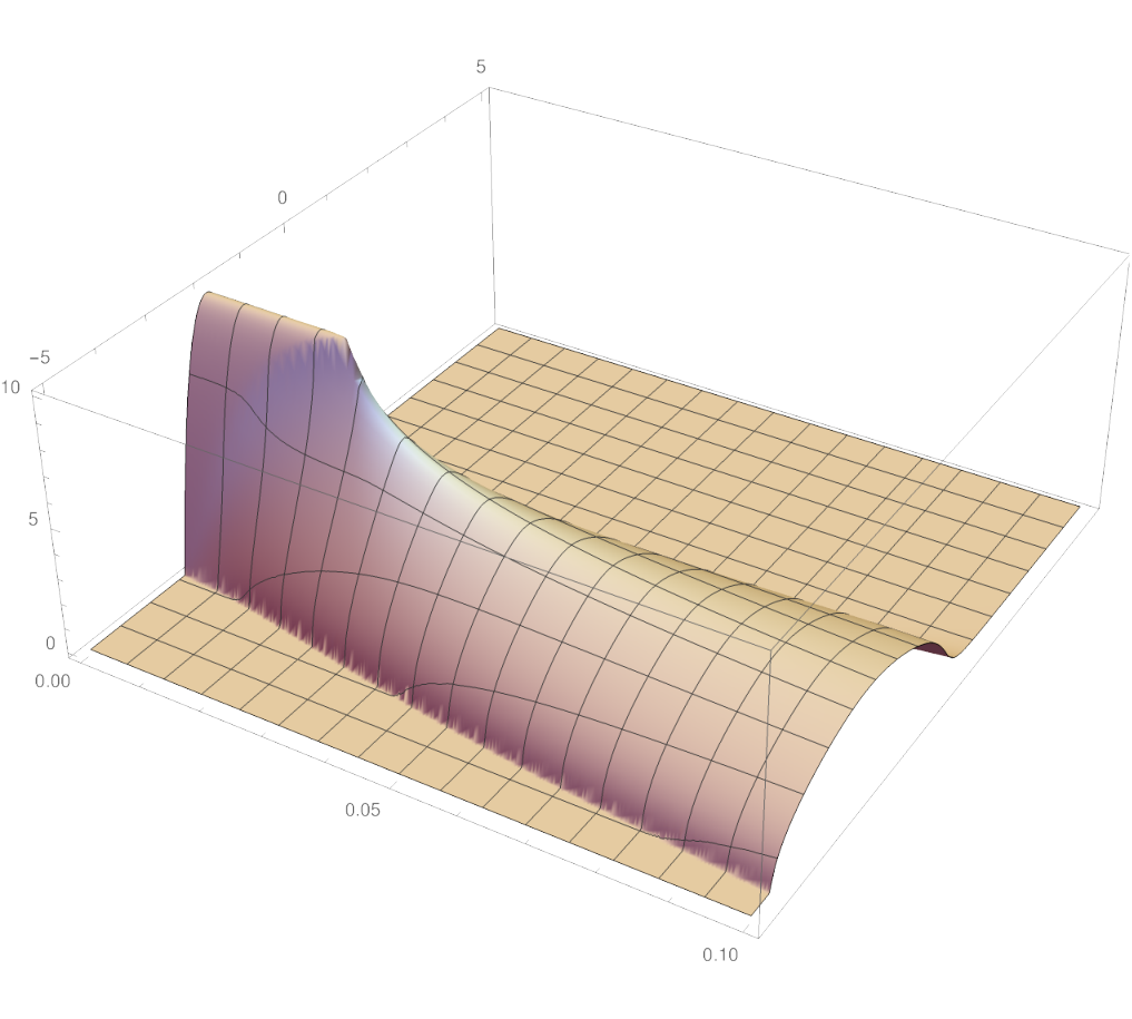
Refer to caption
Refer to caption
Figure 7.1: The solution v⁡(t,x)v(t,x) (left) and w⁡(t,x)w(t,x) (right) for t∈[0,0.1]t\in[0,0.1] and x∈[−5,5]x\in[-5,5].

In Figure 7.2 we show that (unscaled) solutions on the longer time interval t∈[0,10]t\in[0,10], where the self-similar behavior becomes visible.

Refer to caption
Refer to caption
Figure 7.2: The solution v⁡(t,x)v(t,x) (left) and w⁡(t,x)w(t,x) (right) for t∈[0,0.1]t\in[0,0.1] and x∈[−5,5]x\in[-5,5].

In Figure 7.3 we show that the rescaled solutions (t,y)↦(1+t)δ​v​(t,(1+t)δ​y)(t,y)\mapsto(1{+}t)^{\delta}v(t,(1{+}t)^{\delta}y) and (t,y)↦(1+t)δ​w​(t,(1+t)δ​y)(t,y)\mapsto(1{+}t)^{\delta}w(t,(1{+}t)^{\delta}y) for t∈[0,1.5]t\in[0,1.5] where convergence into a self-similar profile is already evident. It is clearly seen that ww develops the simple Barenblatt profile cw​max⁡{0,b−y2}c_{w}\max\{0,b{-}y^{2}\} , whereas vv develops the more singular profile cv​max⁡{0,b−y2}1/4c_{v}\max\{0,b{-}y^{2}\}^{1/4} because of κ0/η0=1/4\kappa_{0}/\eta_{0}=1/4.

Refer to caption
Refer to caption
Figure 7.3: Scaled solutions (1+t)δ​v​(t,(1+t)δ​y)(1{+}t)^{\delta}v(t,(1{+}t)^{\delta}y) (left) and (1+t)δ​w​(t,(1+t)δ​y)(1{+}t)^{\delta}w(t,(1{+}t)^{\delta}y) (right) for t∈[0,1.5]t\in[0,1.5] and y∈[−10,10]y\in[-10,10].

7.3 Conjectured longtime behavior for β≠α\beta\neq\alpha

With the transformation (7.3) with δ=1/(2+d​β)\delta=1/(2{+}d\beta) we now find the transformed system

∂τv~\displaystyle\partial_{\tau}\widetilde{v}\> =div(δv~y+eγ​τη0w~β∇v~)with γ=(β−α)dδ,\displaystyle=\mathop{\mathrm{div}}\nolimits\!\big(\delta\,\widetilde{v}\>y+\mathrm{e}^{\gamma\tau}\eta_{0}\widetilde{w}^{\beta}\nabla\widetilde{v}\big)\hskip 20.00003pt\text{with }\gamma=(\beta{-}\alpha)d\delta, (7.9a)
∂τw~\displaystyle\partial_{\tau}\widetilde{w} =div(δw~y+κ0w~β∇w~)+e(γ−d​δ)​τη0w~β|∇v~|2.\displaystyle=\mathop{\mathrm{div}}\nolimits\!\big(\delta\widetilde{w}\,y+\kappa_{0}\widetilde{w}^{\beta}\nabla\widetilde{w}\big)+\mathrm{e}^{(\gamma-d\delta)\tau}\eta_{0}\widetilde{w}^{\beta}|\nabla\widetilde{v}|^{2}. (7.9b)

We consider the cases α>β>0\alpha>\beta>0 and β>α>0\beta>\alpha>0 separately.

Case γ=(β−α)​d​δ>0\gamma=(\beta{-}\alpha)d\delta>0: The chosen scaling leads to the exponentially growing prefactor for the diffusion in (7.9a). Hence it is dominating the concentration term such that we expect for large τ\tau that ∇v​(τ)\nabla v(\tau) is small. This can also be seen by testing (7.9a) by e−d​δ​τ​v​(τ)\mathrm{e}^{-d\delta\tau}v(\tau) which leads to

∬QTe(γ−d​δ)​τ​η0​w~β​|∇v~|2​𝑑y​𝑑τ≤12​‖v~​(0)‖L2​(Rd)2.\iint_{Q_{T}}\!\!\mathrm{e}^{(\gamma-d\delta)\tau}\eta_{0}\widetilde{w}^{\beta}|\nabla\widetilde{v}|^{2}\;\!\mathrm{d}y\;\!\mathrm{d}\tau\leq\frac{1}{2}\|\widetilde{v}(0)\|_{{\mathrm{L}}^{2}(R^{d})}^{2}.

Thus, it is reasonable to expect that v~​(t)\widetilde{v}(t) converges to c​ 1B1/b​(0)​(⋅)c\,\mathbf{1}_{B_{1/b}(0)}(\cdot) while w~\widetilde{w} converges to w~st\widetilde{w}_{\mathrm{st}} as for the case α=β\alpha=\beta.

A proof of this conjecture will be even more difficult, because ∇v​(τ)\nabla v(\tau) must develop a singularity near the boundary of B1/b​(0)⊂ℝdB_{1/b}(0)\subset{\mathbb{R}}^{d} to allow for the convergence v~​(τ)→c​ 1B1/b​(0)​(⋅)\widetilde{v}(\tau)\to c\,\mathbf{1}_{B_{1/b}(0)}(\cdot) in L2​(ℝd){\mathrm{L}}^{2}({\mathbb{R}}^{d}).

Case γ=(β−α)​d​δ<0\gamma=(\beta{-}\alpha)d\delta<0: In this case we expect a different behavior because of the decaying diffusion in the equation for v~\widetilde{v}. For large τ\tau the dominating term in (7.9a) is the transport term div(δ​v~​y)\mathop{\mathrm{div}}\nolimits\big(\delta\widetilde{v}y\big) which is simply due to the similarity rescaling. Hence, for τ>τ0≫1\tau>\tau_{0}\gg 1 one expects v~​(τ,y)≈ed​δ​(t−τ0)​v~​(τ0,eδ⁡(τ−τ0)​y)\widetilde{v}(\tau,y)\approx\mathrm{e}^{d\delta(t-\tau_{0})}\widetilde{v}\big(\tau_{0},\mathrm{e}^{\delta(\tau-\tau_{0})}y\big), which in the original physical coordinates means the same as v⁡(t,x)≈v⁡(t0,x)v(t,x)\approx v(t_{0},x) for t>t0≫1t>t_{0}\gg 1. Thus, it is likely that ‖v⁡(t)‖L22=e−d​δ​τ​‖v~​(τ)‖L22\|v(t)\|_{{\mathrm{L}}^{2}}^{2}=\mathrm{e}^{-d\delta\tau}\|\widetilde{v}(\tau)\|_{{\mathrm{L}}^{2}}^{2} does not converge to 00 for τ=log⁡(t+1)→∞\tau=\log(t{+}1)\to\infty. Consequently, the nondecreasing function E~​(t):=∫ℝdw~​(τ,y)​𝑑y\widetilde{E}(t):=\int_{{\mathbb{R}}^{d}}\widetilde{w}(\tau,y)\;\!\mathrm{d}y is converging to some E~∞∈[E⁡(0),E0]\widetilde{E}_{\infty}\in{[E(0),E_{0}]} with E0=ℰ⁡(v0,w0)E_{0}={\mathcal{E}}(v^{0},w^{0}). There is still a chance that w~\widetilde{w} converges to some w~st\widetilde{w}_{\mathrm{st}} but now with mass E~∞\widetilde{E}_{\infty} instead of E0E_{0}.

8 Parabolic systems in turbulence modeling

The author’s motivation for studying the given class of coupled degenerate parabolic equation comes from turbulence modeling. However, for the sake of a concise presentation the model was simplified considerably, but still keeping the main feature of a velocity-type variable with a degenerate viscosity depending on the energy-like variable, which is now the mean turbulent kinetic energy k≥0k\geq 0 playing the role of ww. We refer to [Lew97, GL∗03, LeL07, DrN09, Nau13, ChL14] for a mathematical exposition of the ideas behind of such a turbulent modeling and to [Wil93, Ch. 4] for a fluid mechanical approach.

We first introduce Prandtl’s model for turbulence and then Kolmogorov’s two-equation model. In both cases, we introduce the full model with the macroscopically mean velocity 𝐮{\mathbf{u}} satisfying the incompressibility div𝐮=0\mathop{\mathrm{div}}{\mathbf{u}}=0, the pressure pp, and the turbulent kinetic energy k≥0k\geq 0. Then, we show that restricting to simple shear flows of the form 𝐮⁡(t,x)=(0,…,0,v⁡(t,x1,…,xd))∈ℝd+1{\mathbf{u}}(t,x)=\big(0,...,0,v(t,x_{1},...,x_{d})\big)\in{\mathbb{R}}^{d+1} we obtain a system that has the form of our coupled system (1.1) with some simple extra terms.

8.1 Kolmogorov’s one-equation model = Prandtl’s model

Prandtl’s one-equation model for turbulence was developed from 1925 to 1945, see [Pra25, Pra46] and the historical remarks about the development of the model in [Nau13, p. 20].

𝐮˙+𝐮⋅∇¯​𝐮−∇¯​p=div¯​(ℓ​k​D¯​(𝐮))+f,div¯​𝐮=0,\displaystyle\dot{\mathbf{u}}+{\mathbf{u}}\cdot\overline{\nabla}{\mathbf{u}}-\overline{\nabla}p=\overline{\mathop{\mathrm{div}}}\big(\ell\sqrt{k}\,\overline{{\mathrm{D}}}({\mathbf{u}})\big)+f,\hskip 10.00002pt\overline{\mathop{\mathrm{div}}}{\mathbf{u}}=0,
k˙+𝐮⋅∇¯​k=κ^​div¯​(ℓ​k​∇¯​k)+ℓ​k​|D¯​(𝐮)|2−a​k​kℓ,\displaystyle\dot{k}+{\mathbf{u}}\cdot\overline{\nabla}k=\widehat{\kappa}\,\overline{\mathop{\mathrm{div}}}\big(\ell\sqrt{k}\,\overline{\nabla}k\big)+\ell\sqrt{k}\,|\overline{{\mathrm{D}}}({\mathbf{u}})|^{2}-a\,\frac{k\sqrt{k}}{\ell},

where a≥0a\geq 0 is a dimensional parameter and ℓ>0\ell>0 is a constant characteristic length that may depend on position (e.g. via the distance to the wall). Moreover, ∇¯\overline{\nabla}, D¯\overline{{\mathrm{D}}}, and div¯\overline{\mathop{\mathrm{div}}} stand for the differential operators in ℝd+1{\mathbb{R}}^{d+1} with d∈{1,2}d\in\{1,2\}.

Looking for shear flows as defined above and assuming that the external force vanishes, i.e. f≡0f\equiv 0, and that kk is independent of xd+1x_{d+1} we obtain the coupled system

v˙=div(η0k1/2∇v),k˙=div(κ0k1/2∇k)+η0k1/2|∇v|2−aℓk3/2\dot{v}=\mathop{\mathrm{div}}\!\big(\eta_{0}k^{1/2}\nabla v\big),\hskip 20.00003pt\dot{k}=\mathop{\mathrm{div}}\!\big(\kappa_{0}k^{1/2}\nabla k\big)+\eta_{0}k^{1/2}|\nabla v|^{2}-\frac{a}{\ell}\,k^{3/2} (8.1)

with η0=ℓ/2\eta_{0}=\ell/2 and κ0=κ^​ℓ\kappa_{0}=\widehat{\kappa}\ell. Clearly, when neglecting the term involving aa, we arrive at our coupled system in the case α=β=1/2\alpha=\beta=1/2.

The case a>0a>0 does not pose any additional problem when constructing solutions. In particular, the term reduces the total energy in the form dd​tℰ(v,k)=−aℓ∫Ωk3/2dx≤0\frac{{\mathrm{d}}}{{\mathrm{d}}t}{\mathcal{E}}(v,k)=-\frac{a}{\ell}\int_{\Omega}k^{3/2}\;\!\mathrm{d}x\leq 0. Hence, the a priori estimates of this equation remain the same, such that existence of weak solutions with k⁡(t,x)≥k¯>0k(t,x)\geq\underline{k}>0 was shown already in [Nau13]. Our existence result for weak solutions in Theorem 6.1 works for p0=2p_{0}=2 because of α=β=1/2\alpha=\beta=1/2.

The general scaling (2.2) leading to (2.6) can still be applied, but to have the same scaling behavior for the terms k˙\dot{k} and k3/2k^{3/2} we have only one choice, namely γ=2\gamma=2 and with α=1/2\alpha=1/2 and 2​δ+α​γ=12\delta+\alpha\gamma=1 we find δ=0\delta=0. Hence, for (v^,w^)=(1t​v,1t2​w)(\widehat{v},\widehat{w})=\big(\frac{1}{t}v,\frac{1}{t^{2}}w\big) we find the rescaled equation

∂τv^−v^\displaystyle\partial_{\tau}\widehat{v}\>-\ \widehat{v} =div(η0k^1/2∇v^),\displaystyle=\mathop{\mathrm{div}}\nolimits\!\big(\eta_{0}\widehat{k}{}^{1/2}\,\nabla\widehat{v}\big), (8.2)
∂τk^−2​k^\displaystyle\partial_{\tau}\widehat{k}-2\widehat{k} =div(κ0k^1/2∇k^)+η0k^1/2|∇v^|2−aℓk^3/2.\displaystyle=\mathop{\mathrm{div}}\nolimits\!\big(\kappa_{0}\widehat{k}{}^{1/2}\nabla\widehat{k}\big)+\eta_{0}\widehat{k}{}^{1/2}\big|\nabla\widehat{v}\big|^{2}-\frac{a}{\ell}\,\widehat{k}{}^{3/2}.

We may still consider the conserved quantities and find the relations

dd​τ​∫Ωv^​𝑑y=∫Ωv^​𝑑y​ and ​dd​τ​∫Ω(12​v^2+k^)​𝑑y=2​∫Ω(12​v^2+k^)​𝑑y−∫Ωaℓ​k^3/2​𝑑y.\frac{{\mathrm{d}}}{{\mathrm{d}}\tau}\int_{\Omega}\!\widehat{v}\;\!\mathrm{d}y=\int_{\Omega}\widehat{v}\;\!\mathrm{d}y\ \text{ and }\ \frac{{\mathrm{d}}}{{\mathrm{d}}\tau}\int_{\Omega}\!\big(\frac{1}{2}\widehat{v}^{2}{+}\widehat{k}\big)\;\!\mathrm{d}y=2\int_{\Omega}\!\big(\frac{1}{2}\widehat{v}^{2}{+}\widehat{k}\big)\;\!\mathrm{d}y-\int_{\Omega}\frac{a}{\ell}\,\widehat{k}^{3/2}\;\!\mathrm{d}y.

Thus, we may expect that (8.2) has steady states (vst,kst)(v_{\mathrm{st}},k_{\mathrm{st}}) with nontrivial kst≥0k_{\mathrm{st}}\geq 0 (but necessarily with ∫Ωvst​𝑑y=0\int_{\Omega}v_{\mathrm{st}}\;\!\mathrm{d}y=0) that correspond to solutions of (8.1) that decay, namely (v⁡(t,x),k⁡(t,x))=(1t​vst​(x),1t2​kst​(x))(v(t,x),k(t,x))=(\frac{1}{t}v_{\mathrm{st}}(x),\frac{1}{t^{2}}k_{\mathrm{st}}(x)).

8.2 Kolmogorov’s kk-ω\omega model

Kolmogorov’s model [Kol42] (see [Spa91] for a translation, sometimes also called Wilcox kk-ω\omega model because of [Wil93]) consists of the Navier-Stokes equation for the velocity 𝐯∈ℝd{\mathbf{v}}\in{\mathbb{R}}^{d} and the pressure pp coupled to two scalar equations, namely for the specific dissipation rate ω>0\omega>0 (or better dissipation per unit turbulent kinetic energy) and the turbulent energy k≥0k\geq 0:

𝐮˙+𝐮⋅∇¯​𝐮+∇¯​p\displaystyle\dot{\mathbf{u}}+{\mathbf{u}}\cdot\overline{\nabla}{\mathbf{u}}+\overline{\nabla}p =μ1​div¯​(kω​D¯​(𝐮)),div¯​𝐮=0,\displaystyle=\mu_{1}\,\overline{\mathop{\mathrm{div}}}\big(\tfrac{k}{\omega}\overline{{\mathrm{D}}}({\mathbf{u}})\big),\hskip 10.00002pt\overline{\mathop{\mathrm{div}}}\,{\mathbf{u}}=0, (8.3a)
ω˙+𝐮⋅∇¯​ω\displaystyle\dot{\omega}+{\mathbf{u}}\cdot\overline{\nabla}\omega =μ2​div¯​(kω​∇¯​ω)−α1​ω2,\displaystyle=\mu_{2}\,\overline{\mathop{\mathrm{div}}}\big(\tfrac{k}{\omega}\overline{\nabla}\omega\big)-\alpha_{1}\omega^{2}, (8.3b)
k˙+𝐮⋅∇¯​k\displaystyle\dot{k}+{\mathbf{u}}\cdot\overline{\nabla}k =μ3​div¯​(kω​∇¯​k)+μ1​kω​|D¯​(𝐮)|2−α2​k​ω.\displaystyle=\mu_{3}\,\overline{\mathop{\mathrm{div}}}\big(\tfrac{k}{\omega}\overline{\nabla}k\big)+\mu_{1}\tfrac{k}{\omega}\,\big|\overline{{\mathrm{D}}}({\mathbf{u}})\big|^{2}-\alpha_{2}k\omega. (8.3c)

The main point is that all quantities are convected with the fluid velocity 𝐯{\mathbf{v}} and that all quantities diffuse with “viscosities” that are proportional to k/ωk/\omega by the dimensionless factors μj>0\mu_{j}>0. There are sink terms in the equations for ω\omega and kk, namely −α1​ω2-\alpha_{1}\omega^{2} and −α2​k​ω-\alpha_{2}k\omega with dimensionless nonnegative constants αj\alpha_{j}. The nonlinearities in system (8.3) are devised in a specific way to allow for a rich scaling group, see [MiN20, Sec. 2].

The existence of weak solutions to the above coupled system is studied in [MiN15, BuM19, MiN20]. However, in both of these papers the construction of the solutions for (8.3) strongly relies on lower bounds on k⁡(t,x)k(t,x). In [MiN15, MiN20] the assumption k0​(x)=k⁡(0,x)≥k∗>0k_{0}(x)=k(0,x)\geq k_{*}>0 a.e. in Ω\Omega was used, whereas [BuM19] shows that the weaker assumption ∫Ω|log⁡k0​(x)|​𝑑x<∞\int_{\Omega}\big|\log k_{0}(x)\big|\;\!\mathrm{d}x<\infty is sufficient.

Here we are interested in solutions that may have compact support, i.e. k⁡(t,x)=0k(t,x)=0 is allowed on a set of positive measure. In those regions the regularizing diffusion terms μjdiv(kω∇⋅)\mu_{j}\mathop{\mathrm{div}}\nolimits(\frac{k}{\omega}\nabla\,\cdot\,) disappear. Thus, we also restrict to shear flows as above:

v˙\displaystyle\dot{v} =μ12div(kω∇v),ω˙=μ2div(kω∇ω)−ω2,\displaystyle=\tfrac{\mu_{1}}{2}\mathop{\mathrm{div}}\nolimits\!\big(\tfrac{k}{\omega}\nabla v\big),\hskip 20.00003pt\dot{\omega}=\mu_{2}\mathop{\mathrm{div}}\nolimits\!\big(\tfrac{k}{\omega}\nabla\omega\big)-\omega^{2}, (8.4)
k˙\displaystyle\dot{k} =μ3div(kω∇k)+μ12kω|∇v|2−akω.\displaystyle=\mu_{3}\mathop{\mathrm{div}}\nolimits\!\big(\tfrac{k}{\omega}\nabla k\big)+\tfrac{\mu_{1}}{2}\,\tfrac{k}{\omega}|\nabla v|^{2}-ak\omega.

The special symmetry of the nonlinearities allows us for more scalings than the Prandtl equation (8.1), because (8.4) only contains dimensionless parameters μj\mu_{j} and aa whereas (8.1) contains the Prandtl length ℓ\ell. We can look for solutions in the following form (cf. (2.2)), where now ω\omega is given by an explicit solution that is independent of vv and kk:

τ=log(t+1),y=(t+1)−δx,and\displaystyle\tau=\log(t{+}1),\hskip 10.00002pty=(t{+}1)^{-\delta}x,\hskip 10.00002pt\text{and}
(v(t,x),ω(t,x),k(t,x))=((t+1)−γ/2v^(τ,y),1t+1,(t+1)−γk^(τ,y)).\displaystyle\big(v(t,x),\omega(t,x),k(t,x))=\big({(t{+}1)^{-\gamma/2}}\>\widehat{v}(\tau,y),\ \frac{1}{t{+}1},\ {(t{+}1)^{-\gamma}}\>\widehat{k}(\tau,y)\big).

If the exponents γ\gamma and δ\delta are chosen with γ+2​δ=2\gamma+2\delta=2 we are lead to the rescaled system

∂τv^−γ2​v^−δ​y⋅∇v^\displaystyle\partial_{\tau}\widehat{v}-\frac{\gamma}{2}\,\widehat{v}-\delta\,y\cdot\nabla\widehat{v} =μ12div(k^∇v^),\displaystyle=\frac{\mu_{1}}{2}\mathop{\mathrm{div}}\nolimits(\widehat{k}\nabla\widehat{v}), (8.5a)
∂τk^−γ​k^−δ​y⋅∇k^\displaystyle\partial_{\tau}\widehat{k}-\gamma\,\widehat{k}-\delta\,y\cdot\nabla\widehat{k} =μ3div(k^∇k^)+μ12k^|∇v^|2−αk^.\displaystyle=\mu_{3}\mathop{\mathrm{div}}\nolimits(\widehat{k}\nabla\widehat{k})+\frac{\mu_{1}}{2}\widehat{k}|\nabla\widehat{v}|^{2}-\alpha\,\widehat{k}. (8.5b)

The case (γ,δ)=(2,0)(\gamma,\delta)=(2,0) can be applied in bounded domains Ω\Omega and it corresponds to the the case in the Prandtl equation. Clearly, we are in the case α=β=1\alpha=\beta=1 with two additional linear terms, namely v~\widetilde{v} and (2−a)​k~(2{-}a)\widetilde{k}. Thus, the existence theory of very weak solutions in Theorem (6.3) only applies in the case μ1=2​μ2\mu_{1}=2\mu_{2}.

For the case δ>0\delta>0 we consider Ω=ℝd\Omega={\mathbb{R}}^{d}, and the rescaled momentum V⁡(v^,k^)=∫ℝdv⁡(y)​𝑑yV(\widehat{v},\widehat{k})=\int_{{\mathbb{R}}^{d}}v(y)\;\!\mathrm{d}y and the rescaled energy E⁡(v^,k^)=∫ℝd(12​v^2+k^)​𝑑yE(\widehat{v},\widehat{k})=\int_{{\mathbb{R}}^{d}}\big(\frac{1}{2}\widehat{v}^{2}{+}\widehat{k}\big)\;\!\mathrm{d}y now satisfies, along solutions (v^​(τ),k^​(τ))(\widehat{v}(\tau),\widehat{k}(\tau)), the linear relations

OPENdd​τ​V​(v^,k^)=(γ2−𝑑δ))​V​(v^,k^)anddd​τ​E​(v^,k^)=(γ−𝑑δ)​E​(v^,k^)−a​∫ℝdk^​𝑑y.\displaystyle\frac{{\mathrm{d}}}{{\mathrm{d}}\tau}V(\widehat{v},\widehat{k})=\big(\frac{\gamma}{2}-d\delta)\big)V(\widehat{v},\widehat{k})\hskip 10.00002pt\text{and}\hskip 10.00002pt\frac{{\mathrm{d}}}{{\mathrm{d}}\tau}E(\widehat{v},\widehat{k})=(\gamma{-}d\delta)E(\widehat{v},\widehat{k})-a\int_{{\mathbb{R}}^{d}}\widehat{k}\;\!\mathrm{d}y. (8.6)

Because of 2=γ+2​δ2=\gamma+2\delta the case (γ,δ)=(2​d1+d,11+d)(\gamma,\delta)=\big(\frac{2d}{1{+}d},\ \frac{1}{1{+}d}\big) is special as it leads to

(γδ)=11+d​(2​d1)⟹dd​τ​V​(v^,k^)=0​ and ​dd​τ​E​(v^,k^)=d1+d​E​(v^,k^)−a​∫ℝdk^​𝑑y.\tbinom{\gamma}{\delta}=\tfrac{1}{1{+}d}\tbinom{2d}{1}\hskip 10.00002pt\Longrightarrow\hskip 10.00002pt\frac{{\mathrm{d}}}{{\mathrm{d}}\tau}V(\widehat{v},\widehat{k})=0\ \text{ and }\ \frac{{\mathrm{d}}}{{\mathrm{d}}\tau}E(\widehat{v},\widehat{k})=\frac{d}{1{+}d}E(\widehat{v},\widehat{k})-a\int_{{\mathbb{R}}^{d}}\widehat{k}\;\!\mathrm{d}y.

For a<d1+da<\frac{d}{1{+}d} we obtain dd​τ​E​(v^,k^)>0\frac{{\mathrm{d}}}{{\mathrm{d}}\tau}E(\widehat{v},\widehat{k})>0 as long as E⁡(v^,k^)>0E(\widehat{v},\widehat{k})>0, so no steady state can exist. However, for a>d1+da>\frac{d}{1{+}d} one can expect the existence of a family of state states (vst,kst)(v_{\mathrm{st}},k_{\mathrm{st}}) such that V⁡(vst,kst)=V0∈ℝV(v_{\mathrm{st}},k_{\mathrm{st}})=V_{0}\in{\mathbb{R}}.

References

  • [Ama89] H. Amann: Dynamic theory of quasilinear parabolic systems. III: Global existence. Math. Z. 202:2 (1989) 219–250, Erratum Vol. 205, page 331.
  • [BeK90] M. Bertsch and S. Kamin: A system of degenerate parabolic equations. SIAM J. Math. Analysis 21:4 (1990) 905–916.
  • [BFM09] M. Bulíček, E. Feireisl, and J. Málek: A Navier-Stokes-Fourier system for incompressible fluids with temperature dependent material coefficients. Nonl. Analysis RWA 10:2 (2009) 992–1015.
  • [BGO97] L. Boccardo, T. Gallouët, and L. Orsina: Nonlinear eparabolic equations with measure data. J. Funct. Anal. 147:1 (1997) 237–258.
  • [BoG89] L. Boccardo and T. Gallouët: Nonlinear elliptic and parabolic equations involving measure data. J. Funct. Anal. 87:1 (1989) 149–169.
  • [BuM19] M. Bulíček and J. Málek: Large data analysis for Kolmogorov’s two-equation model of turbulence. Nonlinear Analysis: Real World Appl. 50 (2019) 104–143.
  • [CaT00] J. A. Carrillo and G. Toscani: Asymptotic L1L^{1}-decay of solutions of the prous medium equation to self-similarity. Indiana Univ. Math. J. 49:1 (2000) 113–142.
  • [ChL14] T. Chacón Rebello and R. Lewandowski, Mathematical and numerical foundations of turbulence models and applications, Springer, New-York, 2014.
  • [DaG99] R. Dal Passo and L. Giacomelli: Weak solutions of a strongly coupled degenerate parabolic system. Adv. Differ. Equ. 4:5 (1999) 617–638.
  • [DrN09] P.-É. Druet and J. Naumann: On the existence of weak solutions to a stationary one-equation RANS model with unbounded eddy viscosities. Ann. Univ. Ferrara 55 (2009) 67–87.
  • [FeM06] E. Feireisl and J. Málek: On the Navier-Stokes equations with temperature-dependent transport coefficients. Differ. Equ. Nonl. Mech. Art. ID 90616 (2006) 1–14.
  • [GaM98] T. Gallay and A. Mielke: Diffusive mixing of stable states in the Ginzburg-Landau equation. Comm. Math. Phys. 199:1 (1998) 71–97.
  • [GL∗03] T. Gallouët, J. Lederer, R. Lewandowski, F. Murat, and L. Tartar: On a turbulent system with unbounded eddy viscosities. Nonlinear Anal. 52:4 (2003) 1051–1068.
  • [HH∗18] J. Haskovec, S. Hittmeir, P. A. Markowich, and A. Mielke: Decay to equilibrium for energy-reaction-diffusion systems. SIAM J. Math. Analysis 50:1 (2018) 1037–1075.
  • [HyR86] J. M. Hyman and P. Rosenau, Analysis of nonlinear parabolic equations modeling plasma diffusion across a magnetic field, Nonlinear systems of partial differential equations in applied mathematics, Lect. Appl. Math. Vol. 23, 1986, pp. 219–245.
  • [Kol42] A. N. Kolmogorov: The equations of turbulent motion of an incompressible fluid. Izv. Akad. Nauk SSSR Ser. Fiz. 6:1-2 (1942) 56–58.
  • [LeL07] J. Lederer and R. Lewandowski: A RANS 3D model with unbounded eddy viscosities. Ann. I.H. Poincaré Ana. Nonl. 24 (2007) 413–441.
  • [Lew97] R. Lewandowski: The mathematical analysis of the coupling of a turbulent kinetic energy equation to the Navier-Stokes equation with an eddy viscosity. Nonl. Analysis TMA 28 (1997) 393–417.
  • [Lio69] J.-L. Lions, Quelques méthodes de résolution des problèmes aux limites non linéaires, Dunod, Gauthier-Villars, 1969.
  • [Lun95] A. Lunardi, Analytic semigroups and optimal regularity in parabolic problems, Birkhäuser, 1995.
  • [Mie16] A. Mielke, On evolutionary Γ\Gamma-convergence for gradient systems (Ch. 3), Macroscopic and Large Scale Phenomena: Coarse Graining, Mean Field Limits and Ergodicity (A. Muntean, J. Rademacher, and A. Zagaris, eds.), Lecture Notes in Applied Math. Mechanics Vol. 3, Springer, 2016, Proc. of Summer School in Twente University, June 2012, pp. 187–249.
  • [MiM18] A. Mielke and M. Mittnenzweig: Convergence to equilibrium in energy-reaction-diffusion systems using vector-valued functional inequalities. J. Nonlinear Sci. 28:2 (2018) 765–806.
  • [MiN15] A. Mielke and J. Naumann: Global-in-time existence of weak solutions to Kolmogorov’s two-equation model of turbulence. C.R. Acad. Sci. Paris Ser. I 353 (2015) 321–326.
  • [MiN20]   : On the existence of global-in-time weak solutions and scaling laws for Kolmogorov’s two-equation model of turbulence. Z. angew. Math. Mech. (ZAMM) (2020) , Submitted. WIAS preprint 2545, arXiv:1801.02039.
  • [MiS21] A. Mielke and S. Schindler: Existence of similarity profiles for systems of diffusion equations. In preparation (2021) .
  • [Mou16] A. Moussa: Some variants of the classical Aubin–Lions lemma. J. Evol. Eqns. 16:1 (2016) 65–93.
  • [Nau13] J. Naumann: Degenerate parabolic problems in turbulence modelling. Boll. Accad. Gioenia Sci. Nat. Catania 46:376 (2013) 18–43.
  • [Ott01] F. Otto: The geometry of dissipative evolution equations: the porous medium equation. Comm. Partial Diff. Eqns. 26 (2001) 101–174.
  • [Pel14] M. A. Peletier, Variational modelling: Energies, gradient flows, and large deviations, arXiv:1402.1990, 2014.
  • [Pra25] L. Prandtl: Bericht über Untersuchungen zur ausgebildeten Turbulenz. Z. angew. Math. Mech. (ZAMM) 5 (1925) 136–139.
  • [Pra46]   : Über ein neues Formelsystem für die ausgebildete Turbulenz. Nachr. Akad. Wiss. Göttingen, Math. Phys. 1 (1946) 6–19.
  • [Ran95] T. Ransford, Potential theory in the complex plane, London Math. Soc., 1995.
  • [RoH85] P. Rosenau and J. M. Hyman: Analysis of nonlinear mass and energy diffusion. Phys. Rev. A 32 (1985) 2370–2373.
  • [RoH86]   : Plasma diffusion across a magnetic field. Physica D 20 (1986) 444–446.
  • [Rou13] T. Roubíček, Nonlinear partial differential equations with applications (2nd edition), ISNM. International Series of Numerical Mathematics 153, Birkhäuser Verlag, Basel, 2013.
  • [Sim87] J. Simon: Compact sets in the space Lp​(0,T,B)L^{p}(0,T;B). Ann. Mat. Pura Appl. (4) 146 (1987) 65–96.
  • [Spa91] D. B. Spalding: Kolmogorov’s two-equation model of turbulence. Proc. Royal Soc. London Ser. A 434:1890 (1991) 211–216, Turbulence and stochastic processes: Kolmogorov’s ideas 50 years on.
  • [Váz07] J. L. Vázquez, The porous medium equation. mathematical theory, Oxford: Clarendon Press, 2007.
  • [Wie92] M. Wiegner: Global solutions to a class of strongly coupled parabolic systems. Math. Ann. 292:4 (1992) 711–727.
  • [Wil93] D. C. Wilcox, Turbulence modeling for CFD, DCW Industries, 1993.