Entropy stable discontinuous Galerkin methods for the shallow water equations with subcell positivity preservation
Abstract
High order schemes are known to be unstable in the presence of shock discontinuities or under-resolved solution features, and have traditionally required additional filtering, limiting, or artificial viscosity to avoid solution blow up. Entropy stable schemes address this instability by ensuring that physically relevant solutions satisfy a semi-discrete entropy inequality independently of discretization parameters. However, additional measures must be taken to ensure that solutions satisfy physical constraints such as positivity. In this work, we present a high order entropy stable discontinuous Galerkin (ESDG) method for the nonlinear shallow water equations (SWE) on two-dimensional (2D) triangular meshes which preserves the positivity of the water heights. The scheme combines a low order positivity preserving method with a high order entropy stable method using convex limiting. This method is entropy stable and well-balanced for fitted meshes with continuous bathymetry profiles.
1 Introduction
The shallow water equations (SWE) are used to model fluid flows in rivers, open channels, lakes, and coastal regions. One of the most prominent practical applications of the shallow water equations is the numerical prediction of storm surges under extreme weather conditions like hurricanes near coastal regions Abc 2000; Abc 2000; Abc 2000. All of these flows share the fact that vertical scales of the motion are much smaller than horizontal scales. Under certain assumptions Abc 2000, the incompressible Navier–Stokes equations of fluid dynamics can be simplified to the 2D shallow water equations:
| (1.1) | ||||
| (1.2) | ||||
| (1.3) |
where denotes the height of the water measured from the bottom, and denote the velocity in the and directions respectively, denotes the gravitational constant. The bathymetry height is denoted by . The subscript denotes the time derivative, while the subscripts or denote directional derivatives along the and directions, respectively.
Researches on numerical methods for the solution of the shallow water equations have achieved considerable attention in the past two decades. Common numerical methods including the finite difference, the finite volume, and the finite element method have been applied to the shallow water system. This paper focuses on the discontinuous Galerkin (DG) method. Discontinuous Galerkin methods combine advantages of both finite element and finite volume methods, and have been successfully applied to a variety of settings Abc 2000. Discontinuous Galerkin methods can achieve high order accuracy, parallel efficiency, and enjoy more straightforward hp-refinement Abc 2000; Abc 2000. However, high order discontinuous Galerkin methods also introduce issues of stability for problems with shocks or under-resolved solutions. Recent works on entropy stable high order discontinuous Galerkin methods Abc 2000; Abc 2000; Abc 2000 provide a way to address such instabilities. Entropy stable discontinuous Galerkin methods can also be extended to curved meshes, which can be necessary when dealing with complex geometries.
One of the important numerical properties for the shallow water equations is the preservation of steady state solutions, also known as the “lake at rest” condition Abc 2000:
| (1.4) |
A numerical scheme which preserves this steady state is said to be well-balanced Abc 2000; Abc 2000. Schemes that are not well-balanced can generate spurious waves in the presence of varying bottom topographies. Accomplishing this discretely can be challenging because special discretizations of the source terms are required Abc 2000; Abc 2000; Abc 2000.
Another important issue often experienced in numerical simulations of the shallow water equations is the treatment of dry areas, where the water is absent. Dry areas are common in realistic applications of the shallow water equations, such as dam breaks, flooding, and shoreline simulations. Some numerical methods can fail when encountering zero or negative water heights. Various wetting and drying treatments for the shallow water equations have been developed Abc 2000; Abc 2000; Abc 2000; Abc 2000; Abc 2000. Some use mesh adaption to track dry fronts and modify the meshes to fit the wet area. Others exclude dry elements from computation and include them when they are wet again; however, this approach may introduce oscillations and a loss of mass and momentum conservation. Positivity-preserving limiters that average the water height in partially dry elements have been also explored in Abc 2000.
In this paper, we introduce a high order entropy stable numerical method that preserves the positivity of water heights for the shallow water equations through convex limiting. The sections in this paper are organized as follows. We first present a high order entropy stable numerical scheme and entropy stable numerical fluxes for the shallow water equation in 1D and on 2D triangular meshes Abc 2000; Abc 2000; Abc 2000; Abc 2000; Abc 2000 in Sec. 2. Then, we present a low order positivity preserving method Abc 2000 which preserves the positivity of the water heights by using a graph viscosity in Sec. 3. We combine the high order scheme with the low order scheme through a technique called convex limiting Abc 2000 in Sec. 4. If the high order scheme produces negative water heights, the convex limiting procedure blends them with the low order solution to preserve positivity while maintaining high order accuracy in wet areas. Our approach is also different in the sense that we only limit in dry areas without limiting near shocks. We also prove this scheme is well-balanced for meshes which are fitted to dry-wet interfaces. We demonstrate our new method with five numerical experiments that illustrate different properties of our new method in Sec. 5. Conclusions are presented in Sec. 6.
2 High order entropy stable summation-by-parts formulations
2.1 Mathematical assumption and notations
We first introduce some underlying mathematical assumptions and notations for our DG method. For consistency, we reuse notations from Abc 2000, with slight modifications to provide a cleaner discrete formulation. We denote the triangular reference element by with boundary . In 2D, the reference element is a triangle with vertices at , and . We use to represent the th component of the outward normal vector scaled by the face Jacobian on the boundary of the reference element. The space of polynomials up to degree on the reference element is defined as
| (2.1) |
Finally, we denote the dimension of as .
2.2 SBP quadrature rules
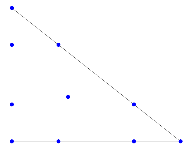
We require SBP-quadrature rules to satisfy certain properties detailed in Abc 2000; Abc 2000. In our numerical experiments, we consider two sets of SBP quadrature points. The first uses 1D Gauss-Legendre quadrature on the edges while the second uses 1D Gauss-Lobatto quadrature on edges. These are shown in the Fig. 1 and 2, respectively. The Gauss-Legendre SBP quadrature rules were introduced in Abc 2000, and the Gauss-Lobatto SBP quadrature rules were introduced in Abc 2000.




2.3 Multi-dimensional SBP operators
We now describe properties satisfied by nodal SBP operators. We assume we are given a degree quadrature rule for the polynomial space , with nodes, , and positive weights . The face quadrature rule is degree and is embedded in the volume nodes. The nodal values of the function on the quadrature points is denoted by:
| (2.2) |
The SBP mass matrix is defined as a diagonal matrix with quadrature weights on the diagonal.
| (2.3) |
We define and to be nodal differentiation matrices associated with the and derivatives Abc 2000; Abc 2000. We also define and to be diagonal surface matrices whose entries are surface quadrature weights scaled by the and components of the outward normal vector.
We have the following definition Abc 2000.
Definition 2.1.
Consider the diagonal mass matrix consisting of quadrature weights
| (2.4) |
A 2D operator is said to be high order accurate and have SBP property if for , the following properties hold:
- •
Let . Then for any .
- •
Given this equivalence, we can now construct an entropy conservative DG-SBP form:
| (2.5) |
where the matrix operations denotes the Hadamard product. denotes the flux matrix and each entry , where is an entropy conservative numerical flux that we will introduce in the next section. denotes the source term. The construction of the high order operators are presented in Abc 2000. The stability analysis of the SBP formulation follows from the results from Abc 2000, and the extension to curved elements can be found in Abc 2000.
2.4 Entropy conservative fluxes for the shallow water equations
The entropy function for the shallow water equations is the total energy of the system Abc 2000; Abc 2000:
| (2.6) |
We also define the entropy variable . The convexity of the entropy function guarantees that the mapping between and is invertible. The entropy variables for the shallow water equations are given explicitly as:
| (2.7) | ||||
| (2.8) | ||||
| (2.9) |
It can be shown as in Abc 2000 that there exists an entropy flux function and entropy potential such that
| (2.10) |
We introduce numerical fluxes for the shallow water equations and describe an entropy conservation discrete formulation Abc 2000; Abc 2000; Abc 2000; Abc 2000. To construct the entropy stable scheme in higher dimensions, we require entropy conservative fluxes as defined in Abc 2000.
Definition 2.2.
Let be a bivariate function which is symmetric and consistent with the flux function , for
| (2.11) |
The numerical flux is entropy conservative if, for entropy variables and , satisfies
| (2.12) | |||
| (2.13) |
The flux can be used to construct entropy conservative and entropy stable finite volume methods, as well as DG methods. Entropy conservative (EC) fluxes for the 2D shallow water equations Abc 2000; Abc 2000; Abc 2000; Abc 2000 are given by
| (2.14) | ||||
| (2.15) |
These fluxes also yield a well-balanced scheme for continuous bathymetry, if the source terms are discretized appropriately Abc 2000. The source terms for the shallow water equations with continuous bottom geometry in the discrete form is defined as
| (2.2) |
By adding local Lax-Friedrichs interface penalization Abc 2000, we can make our numerical scheme entropy stable.
3 Positivity preserving formulation
| In this section, we first describe the steps for constructing a low order positivity preserving DG scheme from Abc 2000 for the shallow water equations. Then, we prove that the low order method preserve the positivity of the water heights. Last, we remark on the sparsity of the low order operators. |
3.1 The low order scheme
We build a low order positivity preserving scheme based on a connectivity graph and the solution of a graph Laplacian problem constructed from the connectivity graph. We present the details of the construction in Appendix A. We assume the same reference element, quadrature points, and discrete operators. We assume the forward Euler time stepping and let denote the time at step and denote the current time step size. Let denote the th diagonal entry global mass matrix, which is diagonal. Suppose we can construct an inviscid approximation of the shallow water equations at some time as follow Abc 2000:
| (3.1) |
for any , the set of all nodes. For any , the set is the neighborhood of the node . We assume that the following property holds: iff . denotes the low order differentiation operator. is described more in details in Sec. 3.2, and its construction is presented in Appendix A. The discrete form of the source term is defined in Eq. 2.2, with replacing the high order differentiation operator with lower order differentiation operator. We also assume that the entries of the low order differentiation operator, , has the following properties:
| (3.2) |
To handle shocks and discontinuous in the solutions, we introduce artificial dissipation using the graph Laplacian associated with the connectivity graph . Let denote the scalar graph viscosity for with the following properties:
| (3.3) |
We define . Now, we can define the low order update as follows:
| (3.4) |
for all . This scheme is conservative in the following sense Abc 2000.
Lemma 3.1.
Assume that , then the scheme (3.4) is conservative, such that the following identity holds for any :
| (3.5) |
Proof.
See Abc 2000. ∎
To enforce the positivity preserving property, we define the graph viscocity coefficients as follows:
| (3.6) |
where
| (3.7) |
is the upper bound for the maximum wave speed. For the shallow water equations, we use the estimate , where and are the and velocity respectively at quadrature point and .
Theorem 3.1.
Proof.
Since we have by property (3.2), we can rewrite the update on the water height term (3.4) as follows:
| (3.8) |
where denotes the flux term that corresponds to the water height. We ignore the source term because the topography or friction terms only affect the momentum equations but not water heights. Then we can introduce the intermediate bar states defined by
| (3.9) |
Notice that we have . We first want to show that if we assume is positive for all , then is also positive. Notice that, for the shallow water equations, the entropy stable numerical fluxes (2.14) are for the water height, where is the velocity of the flow. We can substitute the flux in (3.9) and rewrite the “bar state” as follow:
| (3.10) |
By the definition of , we know that and . Since and are positive, we have
| (3.11) |
Then we can rewrite the low order update on the water height with the bar state as:
| (3.12) | ||||
| (3.13) |
Recall that . If time step satisfies that , then, the term and the terms in (3.13) form a convex combination of two positive water heights. ∎
3.2 Sparsity of the low order operators
One way to build a more accurate lower order numerical scheme is to remove excessive artificial dissipation from the method. In Abc 2000, the author constructed sparse low order operators for tensor product elements in 2D. In this paper, we construct sparse low order operators on triangular elements in 2D. Sparsification can be accomplished by using a sparse connectivity graph to construct low order operators. The sparsity of the graph adjacent matrix directly dictates the sparsity of the differentiation operators . With sparser low order operators, each quadrature node is connected to a fewer number of neighboring nodes. Sparsity reduces the amount of algebraic dissipation since the dissipation coefficient is only non-zero for connected pairs of nodes in the graph. Details on the construction of sparse connectivity graphs are presented in Appendix A.I and numerical results from the low order scheme with different connectivity graphs are presented in Appendix B.
4 Convex limiting
| In this section, we describe the application of convex limiting to combine the low order positivity preserving scheme with high order entropy stable discontinuous Galerkin and apply it to the shallow water equations. This scheme is aligned with the ideas presented in Abc 2000; Abc 2000; Abc 2000. |
In Sec. 3, we showed that the low order solution satisfies the positivity preserving property. In particular, it preserves the positivity of water heights for the shallow water equations. However, it is low order accurate. To recover a high order accurate numerical scheme that also satisfies positivity requirements, we blend the high order and low order updates using “convex limiting”. Convex limiting is only applied to elements where the high order scheme produces zero or negative water heights.
4.1 An overview of convex limiting
We use the superscript H to denote high order terms. By assuming using forward Euler time stepping, we begin by rewriting high order discontinuous Galerkin methods in the form
| (4.1) |
where contains the flux contribution between quadrature points and . We also extend the results to higher order in time with strong-stability preserving Runge-Kutta (SSP-RK). Note that is skew-symmetric, . Subtracting 3.1 from 4.1, we have the following:
| (4.2) |
Let . Then, we can rewrite (4.1) as
| (4.3) |
Note that we have , which implies that . Therefore, the high order and low order updates have the same mass. Our goal is to modify the high order update so that the modified high order update satisfies the positive water heights constraint. We introduce symmetric limiting parameters , for all . We define the limited update as
| (4.4) |
The limiting process is conservative for any choice of symmetric coefficients Abc 2000. Notice that if for all and if for all . Therefore, when all . To obtain a more accurate approximation, we want the limiting coefficients to be as close to 1 as possible while enforcing .
We can rewrite equation 4.4 as
| (4.5) |
where is any set of strictly positive convex coefficients such that , for all . We choose as in Abc 2000. To calculate , we first define for every and :
| (4.6) |
where corresponds to the update on the component of the solution. We set the node-wise limiting factor . With this definition, we can ensure that the water heights stay positive by Theorem 7.21 in Abc 2000. While most of time, finding require a line search, it remains simple for the shallow water equations since we can express explicitly, due to the fact that is a linear function, as follows:
| (4.7) |
With convex limiting, we can ensure that our solution remains positive in water heights throughout a simulation.
An alternative limiting scheme, called element-wise limiting, is also considered in this paper. In this scheme, we have a uniform limiting factor across the same element. We define the element-wise limiting factor . This scheme produces solutions that are closer to the low order positivity preserving scheme than the node-wise limiting scheme because it always has smaller local limiting factors. In practice, solutions from the element-wise limiting scheme are usually bounded further away from 0 and therefore, produce smaller maximum wave speed on the shallow water equations. This has added benefit of allowing us to take larger time steps. We can also prove that, in contrast to the node-wise limiting scheme, the element-wise limiting scheme also preserves the entropy stability of the blended scheme Abc 2000.
4.2 Local implementation
One important and efficient property of our numerical scheme is that it only requires computing limiting factors for the nodes , within the same element, which was first observed in Abc 2000. We use the same entropy stable interface numerical fluxes with a Lax-Friedrichs dissipation in both high order and low order schemes. The resulting fluxes on the boundaries of each element are the same. For example, consider the high order and low order flux matrices for a simple periodic domain in 1D with two elements shown in Fig. 3. Suppose there are three nodes in each element. The non-zero pattern of the matrix from Eq. (4.3) is shown in Fig. 4. We have non-zero entries from the off diagonal block due to the fluxes calculated on the boundaries of each element, namely the terms , , , and . However, these boundary fluxes are the same for both high order and low order updates; therefore corresponding entries in the difference matrix vanish.
As a result, we do not need to implement the convex limiting procedure for the pairs of boundary nodes on neighboring elements. Convex limiting is only required for the pairs of nodes within the same element. With this key property, the implementation of convex limiting is purely local, simplifying the resulting numerical scheme.
5 Numerical results
| In this section, we present some numerical experiments and results in both 1D and 2D to demonstrate the accuracy and stability of the convex limited entropy stable DG scheme. We also add a local Lax-Friedrichs penalization Abc 2000 to all interface fluxes. |
The first experiment is a “lake-at-rest” condition to test the well-balancedness of our scheme in 1D. The second experiment is the parabolic bowl problem in 1D, designed to investigate the convergence rate when positivity preservation is activated. The third experiment is a dam break simulation in 2D from Abc 2000. The last experiment is a wave over a bump in 2D Abc 2000.
All numerical experiments utilize a second order strong-stability preserving Runge-Kutta (SSP-RK) scheme (e.g., Heun’s method) Abc 2000 for time integration. Following the derivation of stable timestep restrictions in Abc 2000, we define the timestep for the high-order scheme to be
| (5.1) |
where is the degree dependent constant in the trace inequality space Abc 2000, and CFL is a user-defined constant. We use CFL = 0.125 for all experiments. For the low order scheme, the timestep is calculated via
| (5.2) |
where is the maximum wave speed calculated with Eq. (3.7) over the entire domain. We define the timestep . To avoid division by zero, we enforce the water height to be above a small positive tolerance in dry areas.
5.1 Lake at rest
The test problem is chosen to verify that the convex limited DG scheme indeed preserves the still water steady state with a non-flat bottom containing a wet/dry interface. The bottom topography is given by the depth function Abc 2000; Abc 2000:
| (5.3) |
The initial data is the stationary solution:
| (5.4) |
A periodic boundary condition is used in this experiment. We compute the solution until T = 1 using 128 uniform cells. The computed surface level and the bottom are plotted in Fig. 5. In order to demonstrate that the lake at rest solution is preserved up to round-off error, we compute the error of the solution. In double precision, the error is 3.56E-15.
We note that well-balancedness is not preserved if the mesh element boundary is not aligned with the wet/dry interface, and that designing a sub-cell well-balanced scheme remains challenging. For example, Abc 2000 presents two numerical schemes, and the scheme which preserves sub-cell well-balanceness is restricted to second order accuracy.

5.2 Translating vortex
We now consider the translating vortex test. We set the domain to be . The exact solution for the vortex at any time is given by Abc 2000; Abc 2000:
| (5.5) | ||||
| (5.6) | ||||
| (5.7) | ||||
| (5.8) |
where
| (5.9) | ||||
| (5.10) | ||||
| (5.11) |
In this example, we set
| (5.12) |
Initially the vortex is located at . In this setup, the vortex propagates to the right along the x-axis. The domain size is chosen to be large enough such that periodic boundary conditions can be used without affecting accuracy.
We use affine triangular meshes for this experiment. We compute the error for the SBP formulation using operators based on Gauss-Legendre quadrature nodes. Recall that the SBP-DG discretization does not correspond to a polynomial approximation space. Thus, to calculate errors for the SBP-DG discretization, we first project the final numerical solution to polynomials of degree . We then use this projection to evaluate the error using a quadrature rule which is exact for at least degree polynomials. The convergence results are presented in Fig. 8. We observe an rate of convergence for the high order method on affine triangular meshes. The method can also be extended to curved triangular meshes Abc 2000.


5.3 Parabolic bowl
The second numerical experiment is used to verify the accuracy and convergence rate of the convex limited DG scheme. For the one-dimensional shallow water equations with a parabolic bottom topography, analytic solutions have been derived by Sampson et al. Abc 2000. For this example, the parabolic bottom is given by
| (5.13) |
where we set and . The computational domain is . The analytical water height for the shallow water equations is given by
| (5.14) |
where and . The exact location of the wet/dry fronts take the form
| (5.15) |
The initial water height is then defined by (5.14). The velocity is initialized to zero. We can use either periodic or wall boundary conditions for this experiment because the water will never reach the boundary. We set the polynomial degree to and run the simulation until with various numbers of uniform elements. We plot the water surface at different times using the node-wise limiting and the element-wise limiting in Fig. 9 and Fig. 10, respectively. We also include the analytical solution to provide a comparison. We observe that the numerical solution matches well with the analytic solution. The element-wise limiting scheme produces smoother solutions than the node-wise limiting scheme. The node-wise limiting scheme produces some spurious oscillations near the dry front, though these oscillations are localized and vanish as we refine the mesh.
We plot the norm of the errors for different polynomial degrees and mesh sizes for the node-wise and element-wise limiting schemes in Fig. 11 and Fig. 12. We observe both schemes have a convergence rate of between and . The node-wise limiting produces larger errors near the dry-wet interface, where the convex limiting scheme pushes towards the low order scheme. The element-wise limiting, on the other hand, produces smaller errors throughout the entire wet domain for lower polynomial degree . Element-wise limiting errors also converge slightly faster than node-wise limiting errors.


5.4 Dam break
This experiment is taken from Abc 2000; Abc 2000. Similar dam break experiments and results can be found in Abc 2000; Abc 2000. We utilize the same physical setting but use triangular meshes instead of quadrilateral meshes. The domain is discretized using a grid of quadrilaterals, and each of them is split into two triangular elements. We set for the polynomial degree. The dam is modeled by imposing reflective boundary conditions along the y-axis with a break between and to allow water to flow through, as shown in Fig. 13.
We start with a zero velocity and constant water heights on both sides of the dam. The bathymetry is set to on both sides. We set the initial water height to be on the left side of the dam and on the right side as shown in Fig. 13.


We plot the solutions from node-wise limiting, element-wise limiting, and the low order positivity preserving method at several different times in Fig. 14 through 17. We observe that the water falling from the left side of the dam to the right produces a wavefront in the lower half of the dam. This wave is discontinuous, so we observe some mesh dependent solution oscillations, but they are localized and do not cause the solution to blow up. The water heights remain positive during the entire numerical experiment. We have also tried simulations with polynomial degrees and . Both of these simulations also remain stable throughout the experiment. The numerical solution of the parabolic dam break problem demonstrates that the entropy stable numerical method remains robust in the presence of shock discontinuities, while the use of convex limiting preserves positive water heights.
We compare the solutions from all three methods. We observe that the results from the node-wise limiting and the element-wise limiting schemes are very similar. They both become wavy near the right boundary. The results from the low order positivity preserving method are much more dissipative than the results from the convex limited schemes. The node-wise limiting scheme produces slightly larger oscillations; however, these oscillations may not be physical as they are not observed in other reference solutions in the literature Abc 2000; Abc 2000. The numerical results from the element-wise limited scheme are more consistent with reference solutions from the literature. This may be due to the fact that an element-wise constant limiting factor preserves a semi-discrete entropy inequality Abc 2000.


5.5 Wave over a bump
The last experiment we perform is a 2D simulation of a wave passing over a bump. The bottom geometry is modeled by a Gaussian bump with a height such that the bump is never entirely submerged. This experiment provides a test of how our numerical solution handles a persistent dry area. We use polynomial degree with a total of 8192 () elements. This experiment runs on the domain with periodic boundary conditions. The bottom topography is given by the following expression:
| (5.16) |
and the initial condition for this experiment is
| (5.17) | ||||
| (5.18) |


We run this experiment up to time T = 1 and plot numerical solutions from three different schemes. In Fig. 19 through Fig. 22, we present the solutions from node-wise limiting scheme, element-wise limiting scheme, and the lower order positivity preserving scheme. For all schemes, we observe that the wave propagates along the -axis, hits the bump and splits, and converges after passing it. We notice that our solution contains small oscillations at the wavefront but never blows up. The water height remains positive even in the presence of a dry area throughout the entire experiment. We observe that the results from the node-wise limiting scheme are very similar to the results from the element-wise limiting scheme for this problem.


6 Conclusions
In this paper, we have presented a high order entropy stable positivity-preserving numerical scheme based on DG methods for the shallow water equations in 1D and on 2D with triangular meshes. This numerical method can preserve the positivity of water heights under an appropriate time step restriction. We apply the convex limiting technique on a low order positivity preserving method and a high order nodal SBP method to obtain this final scheme. This method can achieve high order of accuracy away from dry areas while remaining stable at the wet-dry front. We provide both 1D and 2D numerical experiments to demonstrate our theoretical findings.
Acknowledgement
Authors Xinhui Wu and Jesse Chan gratefully acknowledge support from the National Science Foundation under awards DMS-1719818, DMS-1712639, and DMS-CAREER-1943186.
Author Nathaniel Trask acknowledges funding under the Collaboratory on Mathematics and Physics-Informed Learning Machines for Multiscale and Multiphysics Problems (PhILMs) project funded by DOE Office of Science (Grant number DE-SC001924) and the DOE Early Career program. Sandia National Laboratories is a multi-mission laboratory managed and operated by National Technology and Engineering Solutions of Sandia, LLC., a wholly owned subsidiary of Honeywell International, Inc., for the U.S. Department of Energy’s National Nuclear Security Administration under contract DE-NA0003525. This paper describes objective technical results and analysis. Any subjective views or opinions that might be expressed in the paper do not necessarily represent the views of the U.S. Department of Energy or the United States Government.
Appendix A: Construction of low order operators
In this appendix, we describe the procedures to compute lower order operators. We use a meshfree approach on the SBP nodes. We start by building a connectivity graph on the SBP nodes. Then, we solve a graph-Laplacian problem based on the connectivity graph to form the low order operators.
A.I Construction of sparse connectivity graph
To construct the low order operator , we need to introduce a connectivity graph. This connectivity defines the adjacency matrix from the previous section. We first use uniform radius to define to determine the neighbors of each node, such that node if the distance between node and is less or equal to the radius . However, this approach is less well suited to non-uniform node distributions, which is the case for the Gauss-Legendre quadrature node and Gauss-Lobatto quadrature nodes shown in Fig. 1 and 2, respectively. Then, we investigate the scaling of the radii calculated from coefficient and the quadrature weight of the node raised to some power. So now the radius for node can be written as
| (A.1) |
where is the quadrature weight of the node and is some power. With our experimental approach, we test many different combinations of and and discover that and would produce sparsest connectivity graph. For illustration, we plot the circles with radii on nodes with different quadrature weights in Fig. 23. The red circles define the neighborhoods of nodes. We observe that nodes with greater weights form neighborhoods with larger radii.
Notice that we still need the low order operator constructed from this connectivity graph to satisfy the requirements in (3.2). Therefore, can not be arbitrarily small. In Fig. 24, we notice that the smaller radius can produce a much sparser low order operator by reducing the number of connected nodes. Sparsity can increase the accuracy of the algorithm. It also improves the computing speed because of the fewer number of non-zero terms in the matrix.


A.II Meshfree construction of low order summation-by-parts matrices
This setup defines an undirected finite graph , where the vertices consist of all the quadrature points. is an edge of the graph, i.e., , iff and . We use (V, E) to refer to the connectivity graph. Let denote the radius of a ball. Then we define a adjacency matrix where , for if the distance between node and is less or equal to and otherwise. iff , We let , the number of nodes adjacent to node .
We first build a mesh-free low order differentiation operator in the th coordinate direction with the summation-by-part property. We require that
| (A.2) |
| (A.3) |
We can rewrite Eq. (A.2) as
| (A.4) |
where is skew-symmetric. We assume that for entries and of some “potential” vector . Enforcing then implies that
| (A.5) |
This is equivalent to a Neumann-type graph-Laplacian problem in Abc 2000. We can define the graph Laplacian matrix , where is the diagonal degree matrix whose entries are the degrees of each vertex. Then (A.5) can be written as , and we solve the graph Laplacian problem subject to , where . We solve the system with Lagrange multiplier and use the entries in vector to define the entries in . Last, we use Eq. (A.4) to obtain the differential operator .
Appendix B: Effect of sparsity of the low order operators on numerical dissipation
In this appendix, we demonstrate the effect of sparsity of low order operators on the quality of the low order positivity-preserving numerical solution. We test the low order scheme with low order operators constructed using different connectivity graphs. We utilize a sine wave initial condition on mesh defined on with a grid with periodic boundary conditions and a flat bottom topography. The initial conditions for this experiment are
| (B.6) |
We run each low order scheme up to with different connection radii and present the results in Fig. 25. We observe that the solutions become more dissipative as the radii increases. The larger becomes, the more connected the quadrature nodes are, resulting in graph viscosity being applied between more pairs of nodes. Choosing smaller values for results in sparser low order operators, which sharpens the numerical solution and avoids introducing extraneous artificial dissipation.


References
- Abc [2000] Clint N Dawson, Ethan J Kubatko, Joannes J Westerink, Corey Trahan, Christopher Mirabito, Craig Michoski, and Nishant Panda. Discontinuous Galerkin methods for modeling hurricane storm surge. Advances in Water Resources, 34(9):1165–1176, 2011.
- Abc [2000] Muhammad Akbar and Shahrouz Aliabadi. Hybrid numerical methods to solve shallow water equations for hurricane induced storm surge modeling. Environmental modelling & software, 46:118–128, 2013.
- Abc [2000] Niklas Wintermeyer, Andrew R Winters, Gregor J Gassner, and Timothy Warburton. An entropy stable discontinuous Galerkin method for the shallow water equations on curvilinear meshes with wet/dry fronts accelerated by GPUs. Journal of Computational Physics, 375:447–480, 2018.
- Abc [2000] Clint N Dawson and Christopher M Mirabito. The shallow water equations. University of Texas, Austin, 29, 2008.
- Abc [2000] Jan S Hesthaven and Tim Warburton. Nodal discontinuous Galerkin methods: algorithms, analysis, and applications. Springer Science & Business Media, 2007.
- Abc [2000] Clint Dawson and Jennifer Proft. Discontinuous and coupled continuous/discontinuous Galerkin methods for the shallow water equations. Computer Methods in Applied Mechanics and Engineering, 191(41-42):4721–4746, 2002.
- Abc [2000] Francis X Giraldo, Jan S Hesthaven, and Tim Warburton. Nodal high-order discontinuous Galerkin methods for the spherical shallow water equations. Journal of Computational Physics, 181(2):499–525, 2002.
- Abc [2000] Niklas Wintermeyer, Andrew R Winters, Gregor J Gassner, and David A Kopriva. An entropy stable nodal discontinuous Galerkin method for the two dimensional shallow water equations on unstructured curvilinear meshes with discontinuous bathymetry. Journal of Computational Physics, 340:200–242, 2017.
- Abc [2000] Jesse Chan. On discretely entropy conservative and entropy stable discontinuous Galerkin methods. Journal of Computational Physics, 362:346–374, 2018.
- Abc [2000] Xiao Wen, Wai Sun Don, and Yulong Xing. Entropy Stable Discontinuous Galerkin Method for Shallow Water Equations. Submitted to Journal of Scientific Computing, 2020.
- Abc [2000] Gregor J Gassner, Andrew R Winters, and David A Kopriva. A well balanced and entropy conservative discontinuous Galerkin spectral element method for the shallow water equations. Applied Mathematics and Computation, 272:291–308, 2016.
- Abc [2000] Sebastian Noelle, Yulong Xing, and Chi-Wang Shu. High-order well-balanced finite volume WENO schemes for shallow water equation with moving water. Journal of Computational Physics, 226(1):29–58, 2007.
- Abc [2000] Ulrik S Fjordholm, Siddhartha Mishra, and Eitan Tadmor. Well-balanced and energy stable schemes for the shallow water equations with discontinuous topography. Journal of Computational Physics, 230(14):5587–5609, 2011.
- Abc [2000] Yulong Xing. Exactly well-balanced discontinuous Galerkin methods for the shallow water equations with moving water equilibrium. Journal of Computational Physics, 257:536–553, 2014.
- Abc [2000] Chris Nielsen and Colin Apelt. Parameters affecting the performance of wetting and drying in a two-dimensional finite element long wave hydrodynamic model. Journal of Hydraulic Engineering, 129(8):628–636, 2003.
- Abc [2000] Yulong Xing, Xiangxiong Zhang, and Chi-Wang Shu. Positivity-preserving high order well-balanced discontinuous Galerkin methods for the shallow water equations. Advances in Water Resources, 33(12):1476–1493, 2010.
- Abc [2000] Emmanuel Audusse and Marie-Odile Bristeau. A well-balanced positivity preserving “second-order” scheme for shallow water flows on unstructured meshes. Journal of Computational Physics, 206(1):311–333, 2005.
- Abc [2000] Yulong Xing and Xiangxiong Zhang. Positivity-preserving well-balanced discontinuous Galerkin methods for the shallow water equations on unstructured triangular meshes. Journal of Scientific Computing, 57(1):19–41, 2013.
- Abc [2000] Yi Jiang and Hailiang Liu. An invariant-region-preserving (IRP) limiter to DG methods for compressible Euler equations. In XVI International Conference on Hyperbolic Problems: Theory, Numerics, Applications, pages 71–83. Springer, 2016.
- Abc [2000] Tianheng Chen and Chi-Wang Shu. Review of entropy stable discontinuous galerkin methods for systems of conservation laws on unstructured simplex meshes. CSIAM Transactions on Applied Mathematics, 1(1):1–52, 2020.
- Abc [2000] Tianheng Chen and Chi-Wang Shu. Entropy stable high order discontinuous Galerkin methods with suitable quadrature rules for hyperbolic conservation laws. Journal of Computational Physics, 345:427–461, 2017.
- Abc [2000] Xinhui Wu, Ethan J Kubatko, and Jesse Chan. High-order entropy stable discontinuous Galerkin methods for the shallow water equations: curved triangular meshes and GPU acceleration. Computers & Mathematics with Applications, 82:179–199, 2021.
- Abc [2000] Xinhui Wu and Jesse Chan. Entropy stable discontinuous Galerkin methods for nonlinear conservation laws on networks and multi-dimensional domains. Journal of Scientific Computing, 87(3):1–34, 2021.
- Abc [2000] Jean-Luc Guermond and Bojan Popov. Invariant domains and first-order continuous finite element approximation for hyperbolic systems. SIAM Journal on Numerical Analysis, 54(4):2466–2489, 2016.
- Abc [2000] Jean-Luc Guermond, Bojan Popov, and Ignacio Tomas. Invariant domain preserving discretization-independent schemes and convex limiting for hyperbolic systems. Computer Methods in Applied Mechanics and Engineering, 347:143–175, 2019.
- Abc [2000] Jared Crean, Jason E Hicken, David C Del Rey Fernández, David W Zingg, and Mark H Carpenter. Entropy-stable summation-by-parts discretization of the Euler equations on general curved elements. Journal of Computational Physics, 356:410–438, 2018.
- Abc [2000] Michael S Mock. Systems of conservation laws of mixed type. Journal of Differential equations, 37(1):70–88, 1980.
- Abc [2000] Travis C Fisher and Mark H Carpenter. High-order entropy stable finite difference schemes for nonlinear conservation laws: Finite domains. Journal of Computational Physics, 252:518–557, 2013.
- Abc [2000] Gregor J Gassner, Andrew R Winters, Florian J Hindenlang, and David A Kopriva. The BR1 scheme is stable for the compressible Navier–Stokes equations. Journal of Scientific Computing, 77(1):154–200, 2018.
- Abc [2000] Gregor J Gassner, Andrew R Winters, and David A Kopriva. Split form nodal discontinuous Galerkin schemes with summation-by-parts property for the compressible Euler equations. Journal of Computational Physics, 327:39–66, 2016.
- Abc [2000] Eitan Tadmor. The numerical viscosity of entropy stable schemes for systems of conservation laws. I. Mathematics of Computation, 49(179):91–103, 1987.
- Abc [2000] Eitan Tadmor. Entropy stability theory for difference approximations of nonlinear conservation laws and related time-dependent problems. Acta Numerica, 12:451–512, 2003.
- Abc [2000] Mark H Carpenter, Travis C Fisher, Eric J Nielsen, and Steven H Frankel. Entropy Stable Spectral Collocation Schemes for the Navier–Stokes Equations: Discontinuous Interfaces. SIAM Journal on Scientific Computing, 36(5):B835–B867, 2014.
- Abc [2000] Will Pazner. Sparse invariant domain preserving discontinuous Galerkin methods with subcell convex limiting. Computer Methods in Applied Mechanics and Engineering, 382:113876, 2021.
- Abc [2000] Benoit Perthame and Youchun Qiu. A variant of Van Leer’s method for multidimensional systems of conservation laws. Journal of Computational Physics, 112(2):370–381, 1994.
- Abc [2000] Benoit Perthame and Chi-Wang Shu. On positivity preserving finite volume schemes for Euler equations. Numerische Mathematik, 73(1):119–130, 1996.
- Abc [2000] Sebastian Hennemann, Andrés M Rueda-Ramírez, Florian J Hindenlang, and Gregor J Gassner. A provably entropy stable subcell shock capturing approach for high order split form DG for the compressible Euler equations. Journal of Computational Physics, 426:109935, 2021.
- Abc [2000] Endre Süli and David F Mayers. An Introduction to Numerical Analysis. Cambridge university press, 2003.
- Abc [2000] Jesse Chan, Zheng Wang, Axel Modave, Jean-François Remacle, and Tim Warburton. GPU-accelerated discontinuous Galerkin methods on hybrid meshes. Journal of Computational Physics, 318:142–168, 2016.
- Abc [2000] Timothy Warburton and Jan S Hesthaven. On the constants in hp-finite element trace inverse inequalities. Computer methods in applied mechanics and engineering, 192(ARTICLE):2765–2773, 2003.
- Abc [2000] Qiuhua Liang and Fabien Marche. Numerical resolution of well-balanced shallow water equations with complex source terms. Advances in water resources, 32(6):873–884, 2009.
- Abc [2000] Pascal Azerad, Jean-Luc Guermond, and Bojan Popov. Well-balanced second-order approximation of the shallow water equation with continuous finite elements. SIAM Journal on Numerical Analysis, 55(6):3203–3224, 2017.
- Abc [2000] Shinhoo Kang, Francis X Giraldo, and Tan Bui-Thanh. IMEX HDG-DG: A coupled implicit hybridized discontinuous Galerkin and explicit discontinuous Galerkin approach for shallow water systems. Journal of Computational Physics, 401:109010, 2020.
- Abc [2000] Mario Ricchiuto and Andreas Bollermann. Stabilized residual distribution for shallow water simulations. Journal of Computational Physics, 228(4):1071–1115, 2009.
- Abc [2000] Joe Sampson, Alan Easton, and Manmohan Singh. Moving boundary shallow water flow above parabolic bottom topography. Anziam Journal, 47:C373–C387, 2005.
- Abc [2000] Mária Lukácová-Medvid’ová and Eitan Tadmor. On the entropy stability of the Roe-type finite volume methods. In Proceedings of the twelfth international conference on hyperbolic problems, American Mathematical Society, eds. J.-G. Liu et al, volume 67, 2009.
- Abc [2000] Eitan Tadmor and Weigang Zhong. Energy-preserving and stable approximations for the two-dimensional shallow water equations. In Mathematics and computation, a contemporary view, pages 67–94. Springer, 2008.
- Abc [2000] Nathaniel Trask, Pavel Bochev, and Mauro Perego. A conservative, consistent, and scalable meshfree mimetic method. Journal of Computational Physics, 409:109187, 2020.