Deterministic and Stochastic in-host Tuberculosis Models for Bacterium-directed and Host-directed Therapy Combination
Abstract
Mycobacterium tuberculosis infection can involve all immune system components and can result in different disease outcomes. The antibiotic TB drugs require strict adherence to prevent both disease relapse and mutation of drug- and multidrug-resistant strains. To overcome the constraints of pathogen-directed therapy, host-directed therapy has attracted more attention in recent years as an adjunct therapy to enhance host immunity to fight against this intractable pathogen. The goal of this paper is to investigate in-host tuberculosis models to provide insights into therapy development. Focusing on therapy-targeting parameters, the parameter regions for different disease outcomes are identified from an established ODE model. Interestingly, the ODE model also demonstrates that the immune responses can both benefit and impede disease progression, depending on the number of bacteria engulfed and released by macrophages. We then develop two Itô SDE models, which consider the impact of demographic variations at the cellular level and environmental variations during therapies along with demographic variations. The SDE model with demographic variation suggests that stochastic fluctuations at the cellular level have significant influences on (1) the T-cell population in all parameter regions, (2) the bacterial population when parameters located in the region with multiple disease outcomes, and (3) the uninfected macrophage population in the parameter region representing active disease. Further, considering environmental variations from therapies, the second SDE model suggests that disease progression can slow down if therapies (1) can have fast return rates and (2) can bring parameter values into the disease clearance regions.
In-host tuberculosis model, deterministic model, stochastic model, bifurcation analysis
MSC Code: 34C23, 60H10, 92D25
1 Introduction
Tuberculosis (TB) is a major cause of death from infectious diseases globally. It infects one quarter of the world population and claims 1.4 million lives per year (Organization 2020). Even though it is an ancient disease, TB is still formidable due to the spread of drug-resistant strains, which can lead to re-emergence in the regions of the world with smaller TB burdens. The world is at a critical tipping point in the elimination of TB (Organization 2015). The primary strategies to fight against TB are rapid identification, appropriate treatment of infected cases, and continued surveillance to manage outbreaks. It is necessary to incorporate interventions at the population level with a decrease in the disease progression at the individual level.
On an individual basis, the disease outcome varies among clearance, active disease, and latent tuberculosis infection (LTBI) (Gammack et al. 2005,Meermeier & Lewinsohn 2018). In more detail, after the exposure with Mycobacterium tuberculosis (Mtb), a fraction of individuals can eradicate the infecting Mtb pathogens naturally and achieve early clearance. Evidence of early clearance in Uganda (Bark et al. 2017) ranges from to (Cobat et al. 2009). Another roughly — of infected individuals rapidly progress to active disease (fast progression) (Sud et al. 2006) after initial exposure, while the majority of infected individuals stay in latent tuberculosis infection status (Lin & Flynn 2010). The global prevalence of LTBI is estimated about (Cohen et al. 2019). Patients with LTBI status have Mtb pathogens present but show no clinical symptoms. However, endogenous reactivation (slow progression) can still induce disease progression to active TB for the rest of their life at about (Organization 2020). Moreover, even though only about one in ten LTBI cases become active, this progression contributes to approximately of active disease cases globally (Schwartz et al. 2020). One of the causes of different disease outcomes and disease progression is an impaired host immune system, particularly in the case of immune suppression by HIV and malnutrition. For HIV infected individuals, the damage to the innate immunity increases macrophage turnover (Hasegawa et al. 2009), and the impairment of adaptive immune system reduces CD4+ T cell counts and the baseline monocyte to lymphocyte ratio (Naranbhai et al. 2013). For malnourished TB patients (such as vitamin D deficiency), delayed recovery and higher mortality rates are reported (Gupta et al. 2009).
The development of the antibiotic TB medication streptomycin started in 1943 (1). Nowadays, LTBI and active TB disease can be treated. The anti-TB drug treatments include four first-line drugs, isoniazid (INH), rifampin (RIF), pyrazinamide (PZA), and ethambutol (EMB), which either act as a bactericide or a bacteriostatic agent. Even though the anti-TB regimens have an up-to- efficacy (Conde & Lapa 2011), treatment effectiveness differs according to the adherence of strict routine conditions (Mitnick et al. 2009). If patients stop using medications too soon, take incorrect medication, or use irregular medication, the Mtb bacteria may still live, which can cause disease relapse and mutation of antibiotic-resistant strains. The antibiotic-resistant Mtb strains are much more difficult to treat. Frustrated by antimicrobial resistance and strict treatment adherence, researchers have focused on host-cell factors to inhibit Mtb pathogens’ replication or persistence and promote host immune responses against the invading pathogens.
Host-directed therapies (HDTs) are emerging as adjunctive therapies lately (Zumla et al. 2020). HDTs aim at the enhancement of long-term treatment outcome and the functional cure of persistent Mtb bacteria. Examples of adjunctive HDTs include (1) nonsteroidal anti-inflammatory drugs, such as ibuprofen, to prevent host inflammatory responses, (2) vitamins and dietary supplements, such as vitamin D, to promote immune response, (3) and other drugs to reduce intracellular bacillary load of Mtb (Zumla et al. 2015). To facilitate the development of novel therapy strategies, identification of the key mechanisms of the interactions between Mtb bacteria and host immune response is crucial. This serves as the motivation of this project.
Mathematical modeling has been a fundamental research tool for studying complex dynamics and identifying the underlying causal factors. The papers (Wigginton & Kirschner 2001, Marino & Kirschner 2004, Gammack et al. 2005 and Sud et al. 2006) are starts of in-host modeling regarding immunology of Mtb infections and host-immune response. These previous works successfully combined both bacterial and immune response mechanisms and developed models of Mtb-host interactions to identify the key factors for various disease outcomes through deterministic models. The study of how stochastic variations affecting in-host dynamics has still fallen short. This may be due to the high model complexity. The previous in-host modeling work contains a large number of equations and parameters, which put a big challenge on the identification of significant model parameters driving the disease progression.
In this project, we adopt an established in-host TB infection model (Du et al. 2017), which incorporates the essential bacterial and immune response mechanisms in a four-dimensional deterministic system with eighteen parameter values and successfully generates all disease outcomes including clearance, LTBI, and active disease. In this contribution, however, Du et al. employed and analyzed only an asymptotic version of the model that neglects the effects of the CD4 T-cell population. Then, the papers (Zhang 2020, Zhang et al. 2020, and Zhang et al. 2021) present rigorous mathematical analyses on a reduced model and the original full model, respectively. In this paper, we focus on the driving factors and consider the stochastic variations on demographic variables (including Mtb pathogen and immune cells populations) and on environmental variables (including the identified driving factors) to explore their influences on disease progression.
The paper is organized as follows. In the rest of section 1, we present an established deterministic Mtb-host model and its basic mathematical properties. In section 2, we formulate two stochastic models considering demographic variations and environmental variations. In section 3, we delimit the parameter regions according to different disease outcomes through bifurcation analysis. We further demonstrate the stochastic influences on each parameter region. In section 4, we investigate the speed of the disease progression under combination therapies. The paper ends with a conclusion and discussion in section 5.
1.1 Mtb-host Dynamics
Mtb infection most frequently happens in the respiratory tract, particularly the lung (pulmonary TB), and the regional lymph nodes. When Mtb are inhaled into the lungs and taken up by resident alveolar macrophages, these bacteria start to multiply and make alveolar macrophages their main target. If receiving adequate stimulation for activation, macrophages can effectively ingest and destroy their phagocytized bacteria. Otherwise, the phagocytized bacteria reproduce inside their host macrophages. The host macrophages are eventually unable to be activated due to the increased phagocytized bacteria load, and become chronically infected. The chronically infected macrophages, which are unable to kill their intracellular bacteria, ultimately either undergo programmed cell death ( i.e., apoptosis or necrosis) due to an excessive intracellular bacterial load or are destroyed through T-cell-mediated immune responses. Both processes lead to the death of chronically infected macrophages, which release intracellular bacteria to the extracellular environment. These extracellular bacteria again are engulfed by activated macrophages and result in either bacterial elimination or chronically infected macrophages. The initiation of the T-cell-mediated immunity starts from the infected front-line innate immune cells, including macrophages and dendritic cells. These innate immune cells migrate from the lung to the draining lymph node and activate naive T cells with the present of Mtb. Activated effector and memory T cells then travel back to the lung infection site, engage in granuloma formation, and control the infection. The major elements of the host immune response against Mtb infection involve macrophages, T lymphocytes, and Mtb bacteria.
1.2 In-host Deterministic Model
Our model describes the host-pathogen dynamics for human Mtb infection in lung tissue. Since the site of infection is the human lung, we focus on the interactions among Mtb bacteria (the pathogens), macrophages (Mtb ideal target cells), and lymphocytes (especially T cells for cell-mediated, cytotoxic adaptive immunity). The measurement for all cells is taken in units per milliliter. The 4-dimensional model (1.1) describes the dynamics of the uninfected and infected macrophages, the Mtb bacteria , and the CD4+ T cells . In this model, we consider the effects from CD8+ T cells (cytotoxic T cells or CTL) and cytokines indirectly. The model was developed by Du et al. 2017, analyzed by Zhang et al. 2020 and Zhang et al. 2021. We present the model in (1.1) followed by model descriptions. Moreover, we write the parameter descriptions and values in Table 1.
| (1.1) |
| Symbol | Description (Unites) | Value |
|---|---|---|
| recruitment rate of (1/ml day) | ||
| recruitment rate of (1/ml day) | ||
| death rate of (1/day) | ||
| loss rate of (1/day) | ||
| death rate of (1/day) | ||
| infection rate by (1/day) | ||
| bacteria killing rate by rate (1/ml day) | ||
| cell-mediated immunity rate (1/day) | ||
| proliferation rate of (1/day) | ||
| expansion rate of induce by (1/day) | ||
| expansion rate of induce by (1/day) | ||
| saturating factor of expansion related to | ||
| saturating factor of expansion related to | ||
| half-saturation ratio for lysis () | ||
| carrying capacity of (1/ml) | ||
| max MOI of () | ||
| max No. of released by apoptosis (and necrosis) () | ||
| () |
Macrophages.
Uninfected macrophages arrive at the infection site at a constant recruitment rate of and have a finite lifespan with a natural death rate . With the presence of Mtb, uninfected macrophages engulf the bacteria and become chronically infected at a rate without receiving sufficient stimulation for activation. The apoptosis and necrosis of infected macrophages could occur naturally, by bursting induced by the excessive intracellular bacterium load caused by the phagocytized bacteria multiplication, or by receiving the death signal from CD8+ cells. The loss rate of infected macrophages due to natural death and bursting is denoted as .
Since the activation and proliferation of CD8+ T cells require the signal from CD4+ T cells, we consider the cytotoxic action (i.e., CD8+ T cells target intracellular bacteria) is proportional to CD4+ T cell function. Therefore, the ratio of CD4+ T cell to infected macrophage () determines the rate of CD8+ T cells killing infected macrophages (). This rate reaches to its half-maximum at the value of and its maximum at .
Bacteria.
The bacterial population in TB infection is comprised of intracellular and extracellular bacteria. Extracellular bacteria become intracellular or phagocytized through engulfment by a host macrophage. Intracellular bacteria are released and become extracellular when infected macrophages undergo programmed cell death or killed by T cells. We define extracellular bacteria as , whose division is governed by a logistic term with a constant growth rate and a maximal carrying capacity . The death of an infected macrophage releases intracellular bacteria per cell due to natural death and cell bursting, and releases intracellular bacteria per cell due to CD8+ T cell cytotoxic action. With adequate stimulation, uninfected macrophage engulfment can kill the phagocytized bacteria (, assuming the killing rate is ). Otherwise, phagocytosis turns uninfected macrophages into chronically infected (). We assume the engulfment process takes bacteria per macrophage cell.
CD4+ T lymphocytes.
CD4+ T cells play a role in signaling CD8+ T cell activation and replication to eliminate infected macrophages via cytotoxic action. CD4+ T cells also produce cytokines for granuloma formation and infection control. During the TB infection, professional antigen-presenting cells, including macrophages and dendritic cells, travel to lung-draining lymph node to present Mtb antigens to naive T cells and activate them. We assume that CD4+ T cells are activated by (1) infected macrophages with phagocytized bacteria at rate with the saturating factor , and (2) dendritic cells (assumed in proposition to the extracellular bacteria) at rate with the saturating factor . The natural recruitment and death rates of CD4+ T cells are denoted as and .
1.3 Basic Properties of the Deterministic Model
As an airborne disease, TB is transmitted from person to person through airborne particles containing Mtb (i.e. droplet nuclei). The invasion of the infecting Mtb produces immune responses in the host. Early clearance can be achieved if an effective innate immune response successfully eradicate the infecting Mtb before the development of an adaptive response. Otherwise, the infection stays and develops to either an active TB or LTBI. A delayed clearance can still be achieved thanks to adaptive immune responses.
In the previous paper (Zhang et al. 2020), we proved that the solution trajectories stay in a bounded positive quadrant for all positive time and carried out the steady state analysis. We denote the steady state as . If uninfected macrophages phagocytose all extracellular Mtb and kill all the engulfed bacteria through phagocytosis, then no chronically infected macrophages will be generated, and the early infection is eradicated. That means the infection term () is . We then have . Here, denotes the uninfected macrophage population on a quasi-steady state level, is the minimum average lifetime of an infected macrophage ( the loss rate of infected macrophages and the maximum infected macrophage elimination rate by T-cell mediated immune response). The infection then reaches a trivial steady state, . It denotes the clearance of resident bacteria by macrophages with the help of T-cell mediated immune response. If , the existence of bacteria located anywhere other than inside infected macrophages is possible. This infected steady state is , , , and
2 Two Stochastic Models
Randomness is a typical feature in immunology (Wodarz 2007). It prevents us from foreseeing the exact state at a given time during the process of immune responses. However, if the same experiment is repeated a large number of times, we can obtain a certain trend with similar outcomes. For example, the solution of a linear deterministic model represents the expectation of the corresponding stochastic model. However, the solutions of deterministic models fail to provide information about the intrinsic variability in stochastic models. These random variations in immune responses could induce various disease and treatment outcomes in a model with multiple stable equilibriums. We apply multivariate Itô SDEs to model the dynamics of Mtb bacteria and immune cells’ interaction by using the modeling algorithm based on a multivariate continuous Markov chain model (Allen 1999, Allen 2007, Allen 2017,Allen et al. 2008, and Allen et al. 2020).
Two stochastic models are formulated based on demographic variations and environmental variations, respectively. The study of population changes of pathogens and immune cells can be viewed as the study of demography in population dynamics. The dynamics between pathogens and the immune system demonstrate predator-prey interactions. The immune cells, acting as predators, capture and kill their pathogen prey. During this interaction, the sizes of immune cell populations grow. This induces a faster decline in the pathogen population. In the meantime, Mtb pathogens proliferate and evolve survival strategies to avoid the predation from immune cells. Moreover, the infection process turns healthy macrophage cells into infected cells.
We model the changes over time within the cell population processes, such as proliferation, death, immigration, and transition of both immune cells and Mtb bacteria as demographic variations. An SDE model with demographic variations captures the random nature of this cell population birth-death-immigration process. Moreover, the noise-induced demographic variations can cause species collapse/recover between high- and low-abundance equilibriums (Meng et al. 2020) in the ecology system. Analogously, demographic variations could induce the transition between a low-infection state (such as LTBI) and a high-infection state (such as active disease) in the interplay of pathogens and immune system. In addition, the inhabiting environment (such as the individual’s physical factors) also changes and very likely affects the pathogen and host immune cell populations in other random manners, such as the infected macrophage loss rate, cell-mediated immunity rate, macrophages bacteria killing rate, and bacterial proliferation rate. Instead of including additional variables in the existing ODE model, an alternative way to include these environmental variations is modeling the affected parameters as random variables following certain stochastic processes (Allen 1999). These environmental variations happen especially in drug therapy and alter the cellular environment with random manner due to the heterogeneity in individual cell response. This motivates us to develop the second SDE model with both demographic and environmental variations.
2.1 SDE Model with Demographic Variations
To formulate stochastic processes from the underling deterministic model (1.1), the first step is to identify the possible interactions resulting in population changes and their probabilities in a given small-time interval . The summary of these changes is in Table 2. Let , , and . Notice that for the SDE model, it is not necessary to convert the units of continuous random variables, , , , and , from concentration to population size (Allen 2010), since the changes do not need to be integer-valued. It is assumed that intracellular Mtb bacteria are reproduced with an infected macrophage and released only upon the lysis of the infected macrophage. If the death of one unit of the infected macrophage, denoted by , is due to the killing of the cell-mediated immunity, units of Mtb bacteria are released, . If it is caused by excessive intracellular bacterium load, units of Mtb bacteria are released, . Furthermore, a loss of extracellular Mtb bacteria can also be caused by phagocytosis of extracellular Mtb bacteria by uninfected macrophages, . All the possible changes in the small-time interval include these eleven changes in Table 2 and a case of no change, , with the possibility . Notice that the higher order of is neglected.
| State Change | Probability | Description | |
|---|---|---|---|
| 1 | recruitment | ||
| 2 | death | ||
| 3 | infected by | ||
| 4 | loss of and release bacteria | ||
| 5 | killed by cell-mediated immunity and release bacteria | ||
| 6 | Mtb bacteria proliferation | ||
| 7 | extracellular loss due to killing and phagotysis of Mtb | ||
| 8 | T-cell recruitment | ||
| 9 | T-cell activated by | ||
| 10 | T-cell activated by | ||
| 11 | T-cell death |
The stochastic processes are formed from the underling deterministic ODE model (1.1).
In the second step of formulation, omitting the higher-order terms of , we compute the first order approximation of the expectation and the covariance . The approximated expectation of can be expressed as follows
where
is the drift vector, which is the same as the right side of the deterministic ODE model (1.1). Here s are coefficients of the terms of the probabilities for the eleven events in Table 2.
The covariance matrix is a matrix, . Dropping the order term results the approximation to order as follows:
Here, the matrix takes the following form
The nonzero elements of are as follows:
Instead of computing the square root of to find the diffusion matrix, we calculate a matrix , such that . In the matrix , four rows indicate four state variables (, , , and ), eleven columns represent eleven events in Table 2. The nonzero elements in the matrix are as follows:
The Itô SDE model considering the demographic variations has the following form:
| (2.1) |
where the vector , are eleven independent Wiener processes, and , are four elements in the drift vector .
2.2 SDE Model with Demographic and Environmental Variations
Host-directed therapies can modulate host immune pathways. The therapies can also affect the corresponding parameters with random manner. We model these environmental effects by including additional random variables in the SDE model (2.1).
In previous work (Zhang et al. 2021), we identify four parameters, which significantly affect the disease progression. These four parameters are the bacterial proliferation rate , the infected macrophages’ loss rate , the cell-mediated immunity rate and macrophages’ killing rate . We then consider environmental variations on them. We adopt a mean-reverting process (Allen 2007a; Allen 2010), which was modeled to study drug administrations and was shown to fit well with real data. Let , where , , , and , , and , we assume the vector is a vector of continuous, mean-reverting, stochastic processes. Each element of satisfies an Itô stochastic differential equation as follows:
where is the return rate to the mean concentration . Here, denotes the desired therapy result, which is modulated by drug therapies. The timescale for returning to one half of its original level is . Therefore, a larger return rate value implies a shorter return time to the desired therapy outcome. Parameters and can be tuned through drug administration strategies. Moreover, denotes the variability of the corresponding process, and is a vector of four independent Wiener processes. The asymptotic mean and variance of are derived by Allen 2007a and Allen 2010 as follows:
Therefore, to avoid a large variability and maintain a steady-state rate of immunity in therapies, the return rate should be sufficiently large, such that . For the simulations in the next section, we assume , which yields . Therefore, under this assumption, the limiting mean and variance are independent of the return rate , but only associated with the mean rate . The system of Itô SDEs with both demographic and environmental variations is written as follows:
| (2.2) |
where , and , for and . Here, denotes initial conditions, and and , and denote independent Wiener processes.
In the following section, numerical methods are used to approximate the solutions of the proposed SDE models. In our simulations, we apply a straightforward Euler-Maruyama method, and set zero as an absorbing state.


3 Mtb-host Dynamics of the ODE Model and SDE Model with demographic variation
Mtb pathogens are extremely adaptive within a host. Their survival strategies involve multiple underlying mechanisms. Among these mechanisms, we focus on the bacterial proliferation rate , which is the parameter most affected by the first-line antibiotic drugs. We apply numerical bifurcation analyses to delimit the parameter space into four regions. Then we investigate disease clearance, latent infection, and active disease on the ODE model (1.1) in the four identified parameter regions. Furthermore, we study the stochastic fluctuation in cellular levels in each parameter region through approximated stationary distributions from simulations of the SDE model (2.1).
3.1 Multiple Disease Outcomes Derived from Bifurcation Analysis
Bacterial concentration reflects the local bacterial load, which is an important variable associated with Mtb virulence (Smith 2003). The relation between bacterial concentration and its proliferation rate is demonstrated through a 1-dimensional bifurcation diagram in Figure 1 (a). The trivial steady state denoting disease clearance, , exists for all positive values of . But it loses its stability when increases and crosses a branching point (BP) bifurcation (transcritical bifurcation) at /day, where
| (3.1) |
Without infection, a reference value for activated antigen-specific CD4+ T cells expressing CD25 is reported as cells/ml (Bisset et al. 2004), and a reference value for resting and activated macrophages is in the order of cells/ml (Antony et al. 1993 and Schwander et al. 1998). The branching point bifurcation generates a disease established steady state , which denotes the case that intracellular Mtb escape macrophages killing and become extracellular. The bacterial concentration can stabilize at a lower level around cells/ml, if takes a value between two saddle node (LP) bifurcations LPl and LPm. The bacterial concentration can also reach a high-level range cells/ml, if takes a value between the saddle-node bifurcation LPh and the transcritical bifurcation BP. A summary is as follows:
- •
Bistability happens between LPh and LPl. Taking for example, clearance occurs if the initial infection contains a low-level of Mtb bacteria, illustrated by the dotted curve (with , , , and ) in Figure 1 (b). Active disease happens in the case of a high-level of bacteria in the initial infection, represented by the solid curve (with , , , and ) in Figure 1 (c).
- •
- •
The infection will certainly reach to a high-level if , since . Taking for example, a simulated trajectory starting from a low Mtb level and ending at high Mtb level, which is plotted in the dash-dot curve (with , , , and ) in Figure 1 (c).
- •
Disease clearance will certainly be achieved if LPh, Taking , a simulated trajectory showing Mtb bacteria die out is the solid curve (with , , , and ) in Figure 1 (b).
The corresponding bifurcation points are LPl: , LPm: , and LPh: . Hopf bifurcation does not occur for the parameter values in Table 1. Moreover, saddle node bifurcation indicates the creation and destruction of equilibriums. Transcritical bifurcation, in this case, is the intersection of disease-free and infected equilibriums. These two bifurcations are sufficient to predict various disease outcomes, which include clearance, latent infection, and active disease. We, therefore, do not consider higher codimension bifurcations in this project. Instead, we divide the parameter range of the bacterial proliferation into four regions shown in Figure 1 (a), i.e. Region 1: , Region 2: , Region 3: , and Region 4: . In Region 1, only stable disease-free equilibrium exists. The ODE model predicts that the infection will die out eventually. In Regions 2 and 3, the ODE model contains multiple stable equilibriums. Depending on the initial invading bacterial level, multiple disease outcomes may occur. In Region 4, the ODE model has one stable infected equilibrium. It implies that the infection will grow to a high-level eventually.


3.2 Various Disease Outcomes with Demographic Variations in Different Parameter Regions
In Region 2, the disease stays only if a very high dose of bacterium is inhaled, which is shown in Figure 1 (b) and (c) for . The separatrix of different disease outcomes is the unstable equilibrium shown in the dashed blue curves in Figure 1 (a). These dashed blue curves show Mtb concentration increases with the decrease of the value. This indicates that a reduction of the bacterial proliferation rate facilitates the disease progression. For comparison, simulations for the SDE model (2.1) with demographic variations demonstrate disease clearance and active disease, as well, which are shown in Figures 2 and 3. The initial values also determine different disease outcomes. Here, we set the parameter value and fix the other parameter values as in Table 1. Based on 10,000 stochastic realizations of model 2.1, expectations and standard deviations of , , , and stabilizes by roughly days. This indicates that solutions of the SDEs (2.1) approach an approximated distribution by time days. The corresponding simulations in Figure 2(a) start from , , , . Four stochastic realizations along with one ODE solution are plotted in Figure 2(b).
At time days, histograms of approximated stationary distributions for , , , and are plotted in Figures 2(c)-2(f). The histogram of the population in Figure 2(c) fits well with the corresponding normal distribution in the black curve. Moreover, in (3.1) implies that the macrophage concentration is at the uninfected level. The histogram of and are heavily skewed to the right with a peak at zero, which indicates the disease clearance. The histogram of peaks around in (3.1) with a long tail. This indicates the T-cell concentration peaks at the uninfected level, with a large variation.
For another set of initial conditions, , , , , expectations and standard deviations of , , , and , based on 10,000 stochastic realizations, stabilize roughly by days, shown in Figure 3(a). All four stochastic realizations grow along with the ODE solution, shown in Figure 3(b). To end at time days, histograms of approximated stationary distributions for , , , and fit well with the corresponding normal distributions shown in Figures 3(c)-3(f). Moreover, , , , and . This indicates an active disease case.
In Region 3, the disease outcome depends on the inhaled dose of bacteria. The disease clearance is shown in the dash-dot curve in Figure 1 (b). The disease progression to LTBI or active TB is shown in the dashed and dotted curves in Figure 1 (c). Simulation results for SDE model (2.1) in Region 3 show similar predictions for the disease clearance and active disease cases in Region 2. We, therefore, omit these two cases in Region 3 and focus on the additional state with low bacterial level generated from the saddle-node bifurcation LP1. We take parameter value in Region 3. In the ODE model (1.1), the stable low bacterial level equilibrium denoting LTBI is . Starting at , , , , based on 10,000 stochastic realizations, expectations and standard deviations of , , , and stabilize roughly by days, as shown in Figure 4(a). Four sample paths and one corresponding ODE solution are graphed in Figure 4(b). At time days, approximated stationary distributions for , , , and have medians as Median, Median, Median, and Median. Even though the histograms for , , and have skewed shapes, the median values for , , and are close to the stable latent infected equilibrium . Notice that the Median is much larger than . This indicates that the demographic variations significantly affect T-cell population.
In Region 4, the disease will progress to active TB shown in the dash-dot curve in Figure 1 (b) by the ODE model prediction. The nontrivial equilibrium of the ODE model (1.1) at is . Starting at , , , , based on 100,000 stochastic realizations, expectations and standard deviations of , , , and stabilize roughly by days, as shown in Figure 5 (a). Four sample paths blow up along with the ODE solution shown in Figure 5 (b). At time days, the means of approximated stationary distributions for , , and are close to , , and . The mean of is far away from , but the standard deviation of the approximated stationary distribution is large as well. It implies that small exposure to Mtb bacterial is more likely to develop to active disease.
r
(a) (b)

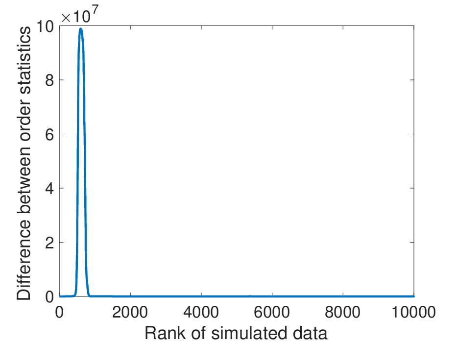
The decreasing parts of the standard deviation curves in Figure 5 (a) indicate that more cell populations converge to their corresponding mean values. Moreover, there are sharp drops at the time roughly between in the standard deviation curves of the same figure. The order statistic Figure 6 suggests that the Mtb concentration, for example, jumps sharply from a low level to a much higher level. This causes the sharp drop in the standard deviation during the time interval . In other words, there are more large values in day than in day . Therefore, the standard deviation is smaller on the later day than the earlier day. It implies that the development of active disease is more likely to happen after day and before day . Interestingly, there are some extremely short bars in the histograms in Figures 5 (c) - (f) that show that there still exists a possibility for disease clearance.
Here are some notes about the SDE simulations in Figures 2, 3, 4, and 5:
- 1.
For each figure, we simulate SDE model (2.1) times. With the obtained sample paths, we calculate their expectations and standard deviations at each time step, then demonstrate the trends of convergence in time-series plots shown in the corresponding subfigures (a). Next, we choose simulation times at which the corresponding expectations and standard deviations converge to their stabilized values, that is , , , for Figures 2, 3, 4, and 5, respectively.
- 2.
- 3.
The baseline parameter values are shown in Table 1. The parameter ranges are provided when variations of parameters are needed. Note that both the baseline values and the ranges of parameters are from existing modeling papers.
- 4.
In Region 2, the ODE model (1.1) contains two stable steady states. We demonstrate disease clearance and active disease under demographic variations in Figures 2 and 3. To generate Figures 2 and 3, we take the same set of parameter values, but different initial conditions (see the figure captions). In Region 3, the ODE model (1.1) has three stable steady states, which represent disease clearance, LTBI, and active disease. SDE simulations for disease clearance and active disease show the similar behavior as in Figures 2 and 3. We, therefore, omit the graphs for these two cases, but only demonstrate the LTBI case in Figure 4. In Region 4, the ODE model (1.1) has only one steady state, which represents active disease. Interestingly, the SDE simulation predicts a possibility for the occurrence of disease clearance (see the tiny bars in histograms in Figure 5). Moreover, the curves representing standard derivations in Figure 5 have decreasing parts with sharp drops. These drops imply that the development of active disease is more likely to happen from the end of the first year to the third year after the initial exposure.
4 Influences of Bacterial and Host Factors on Disease Progression Speed and Combination Therapy Outcomes
In this section, we consider the impact of both the bacterial factor (that is the infected macrophage proliferation rate ) and host factors (including the infected macrophage loss rate , the cell-mediated immunity rate , and macrophages’ bacteria killing rate ) in evaluating the pathogen-directed (antibiotic) therapy with adjunctive host-directed therapies. Previous work (Zhang et al. 2021) sugests that these four parameters have the most statistically significant impacts on model behaviors. We first study the disease dynamics influenced by both the bacterial proliferation rate modulated by pathogen-directed therapy and the host immune components (, , and ) altered by host-directed therapy. Our results suggest that host immune responses can both promote and hinder disease progression. Different disease outcomes depend on the relation between the numbers of Mtb engulfed by and released by macrophages. Considering the stochastic variations from both the cell populations and the adherence to therapies, we investigate the SDE model (2.2) with both demographic and environmental variations to provide insight into the pathogen- and host-directed combination therapy developments. Next, we derive a quadratic relationship between the Mtb spreading speed and the bacterial proliferation rate . Then, we further investigate the disease progression speed under the influences of both pathogen-directed therapy (such as antibiotics affecting ) and host-directed therapy (such as vitamin D affecting , , and ). Our results demonstrate the advantages of the combination therapy.


4.1 Bacterial Concentration Affected by Both the Bacterial Proliferation Rate and Acquired Defects
The analysis results from the ODE model (1.1) in Figure 1 indicate the possibility of disease clearance if the bacterial proliferation rate falls in Region 2, the potential to progress to LTBI or active TB if is in Region 3, and a progression to active TB if is in Region 4 by the ODE model prediction. There also exist values, which guarantee disease clearance. However, this value window is slim and demonstrated in yellow strips in Figure 7. We denote this parameter region for disease clearance as Region 1. The four parameter regions are delimited by saddle node (LP) and transcritical (BP) bifurcations. Two parameter bifurcation analyses were carried out via Matcont (Dhooge et al. 2003). The corresponding bifurcation diagrams are plotted in Figure 7 and illustrate the four regions associated with bacterial proliferation rate and three parameters denoting host immune responses (i.e. , , and ). It is shown that an increase in the loss rate of infected macrophages and a decrease of both the cell-mediated immunity rate and the bacteria killing rate by macrophages impede disease clearance (in Region 1 and 2) and facilitate the disease development (in Region 3 and 4). Note that parameter relations and are taken for the bifurcation analysis under the assumption that macrophages are infected with virulent Mtb and undergo necrosis (Behar et al. 2011). The bifurcation parameter ranges are provided by Du et al. 2017: , , , and . Other than the bifurcation parameters, the other parameter values are taken from Table 1.


Host-directed therapies can modulate host immunity, which in turn tune the associated parameter values. However, these parameter values are influenced by environmental variations due to the patient system’s natural regulation and the stability of adjunct drug concentrations. We then use the second SED model (2.2) that considers both demographic and environmental variations to evaluate the Mtb concentration. The mean values , , , and are taken as the values of , , and in Table 1. We take a return rate relation as for to avoid a large variability during the therapy. Fast and slow return rates are taken as and for simulations of SEDs (2.2). For the case that the pathogen-directed and host-directed therapy combination affects the loss rate of infected macrophages and the bacterial proliferation rate , disease outcomes are predicted by bifurcation analyses of the ODE model (1.1) in Figure 7 (a), and by the second SDE model (2.2) in Figure 8. In Region 2, none of the four Mtb sample paths eventually blow up for the fast return rate, but two of them develop to high Mtb level if the return rate is slow. In Region 3, all four Mtb sample paths blows up. But the sample paths take off slower for the fast return rate than the slow return rate. We do not consider Region 4. Because TB will definitely develop to active disease in this region, we expect therapies will bring parameters away from Region 4. For the therapies targeting parameters and combination and and combination, Figures 8 indicate similar results. Our results suggest that a pathogen-directed and host-directed therapy combination can bring parameter values to Region 2 with a fast return rate (i.e., drug concentration can quickly converge to the desired level). As a result, the patient can spend more time in the disease clearance or latent infection status. This indicates this therapy combination slows down disease progression.
4.2 A Positive Relationship Between the Bacterial Proliferation and the Slope of Disease Progression
Figure 9 shows that the bacterial proliferation rate has a positive relationship with the slope of disease clearance and progression after exposure. More precisely, the slope of bacterium concentration is determined by the dominant eigenvalue. Its linear approximation is a quadratic function of the bacterial proliferation rate . The following derivation is inspired by methods used by Perelson & Nelson 1999 and Yu 2005.
(a) (b)


Tuberculosis infection starts from the inhalation of droplet nuclei carrying Mtb by a healthy individual. The small amount of inhaled tubercle bacilli can be treated as a small positive perturbation of the trivial steady state, . The local stable trivial steady state represents the possible scenario of bacterial clearance, while the unstable trivial steady state means insufficient immune responses fail to clear the infecting bacteria, and thus disease starts to progress. Figure 9 shows that the rate of early clearance and disease progression depends on the bacterial proliferation rate . A higher bacterial proliferation rate results in a slower bacterial decline and a faster disease progress. It also suggests the existence of a threshold value of the bacterial proliferation rate , which separates the early clearance and disease progression in early infection.
Mathematically, the slope of bacteria decline and progression is dependent on the largest eigenvalue of the model (1.1) at the trivial steady state . Consider a general system , where , , and denote state variables, parameters, and a vector of n functions. Suppose that represents the trivial steady state , i.e., . The small amount of invading Mtb pathogens is modeled as a small positive perturbation nearby the trivial steady state, i.e., . The growth of the perturbation indicates the development of the infection, while a decay of corresponds to the disease clearance. The evolution of disease progression is governed by the perturbation of the equation as follows:
If the preceding system is hyperbolic, that is all eigenvalues of have nonzero real parts, then the system can be approximated by the linear system . Further, we assume has distinct eigenvalues with associated eigenvector , i.e., for . We form a matrix , and have . Then the general solution of the linearized system with a chosen initial condition is a linear combination of . That is . Assuming is the dominant eigenvalue (the spectral radius of the matrix ), i.e. , then is the most influential component in the solution basis set of . The evolution of the perturbation is the change of the original variable . It is determined by the dominant eigenvalue . Moreover, if , the perturbation dies out (). The infecting bacteria are eliminated by host immune responses. If , the perturbation grows and the infection develops. The threshold for the infection clearance and establishment is and for .
Taking the general system as the model (1.1) and its trivial equilibrium as . The corresponding eigenvalues are roots of the following characteristic polynomial
| (4.1) |
That is
| (4.2) |
where due to the positiveness of all parameter values. The expression of the preceding equation for and (Zhang et al. 2020) determine the local stability of the trivial equilibrium.
Here, we use the eigenvalues associated with the trivial equilibrium to further investigate the disease progression speed. Extracellular bacteria are introduced into the system by three main ways, extracellular bacterial proliferation, bacterium release by the programmed cell death of infected macrophages, and bacterium release from infected macrophages killed by T-cell mediated immune responses. In early infection, we assume the loss of extracellular Mtb pathogens is caused only by macrophage phagocytosis. We omit the loss of infected macrophages by T-cell mediated immune responses. The per capita rate of macrophage phagocytosis is per uninfected macrophage per bacterium. Considering the (asymptotic) upper bound of the uninfected macrophage , the maximum bacterial loss rate is per bacterium, which is assumed to be greater than the bacterium proliferation rate . Further, assuming that all invading pathogens are phagocytized, that is . This implies , which is equivalent to . Therefore, if , the square root is greater than one, then and are real numbers and have opposite signs. If , then the real parts of and are all negative.
If , a zero-eigenvalue bifurcation occurs at , at which
| (4.3) |
The number of “next generation” infectious Mtb bacteria produced by a single infectious bacterium introduced near the trivial equilibrium is (1) at most by cell proliferation, or (2) and by the death of infected macrophages and T-cell mediated immune response with the probability of and , respectively. In the meantime, phagocytosis can kill at most engulfed bacteria. We assume the uninfected macrophages is at the maximum available level . Therefore, the infection dies out if (i.e., ), but stays if (i.e. , , ). The threshold is . Considering the parameter values in Table 1, the bifurcation analysis shown in Figure 1 (a) shows that the parameter range for latent infected TB (roughly of the total TB infected individuals) is , which is very close to . That is for , (then ), we thus expand the square root in in Equation (4.2) at . This yields
| (4.4) |
(a) (b)


Base on the feasible parameter ranges, holds. We approximate the dominant eigenvalue as a quadratic function of the bacterial proliferation rate . We notice that the dominant eigenvalues determines the changing slope of the bacteria concentration. This implies that if (or ), the Mtb bacterial concentration declines (or grows) in a speed with a quadratic relationship of the bacterial proliferation rate . This speed is slowing down if is approaching to its critical value from both sides, but is speeding up if is moving away from . This is demonstrated by numerical simulations in Figure 9.
4.3 Using Vitamin D as an Adjunctive Therapy
Vitamin D has been shown to promote macrophage maturation, which in turn inhibits the intracellular Mtb growth and enhance antimicrobial immune response (Martino et al. 2019; Arranz-Trullén et al. 2017; Gombart 2009; Rosenberger et al. 2004). A dose-dependent vitamin D induced reduction in Mtb growth can reach (Martineau et al. 2007). The strengthened antimicrobial immune response can be described as an enhanced bacteria killing rate by macrophages, . Equations (4.1) and (4.4) indicate that the dominant eigenvalue has a negative quadratic relationship with . We experiment with different parameter values for and to demonstrate the effect of vitamin D therapy and the combination therapy of antibiotic and vitamin D. We adopt the parameter ranges for and (Du et al. 2017). The simulation in Figure 10 (a) shows that the bacterial decrease slope is much steeper for the solid curve than the dashed one. This supports the idea of using vitamin D as an adjunct therapy for enhanced immune response and obtaining a favorable disease outcome. Figure 10 (b) demonstrates that the dotted curve with a reduced value of shows a faster decay rate. This confirms the promising therapy outcomes of adding vitamin D to modulate the host immune response alongside the antibiotic therapy (Tobin 2015).


Moreover, vitamin D has been suggested to play a pivotal role on interferon- (IFN-)-induced antimicrobial pathway in macrophages against Mtb infection (Fabri et al. 2011). In vitamin D-sufficient sera, IFN- promotes the production of antimicrobial peptides such as Cathelicidin by macrophages (Liu et al. 2006). It in turn enhances the antimicrobial activity by lowing the intracellular survival (Wheelwright et al. 2014). Reducing intracellular Mtb survival induces a reduced level of bacterial release in T-cell mediated cell death. That means a decrease on the values of , which denotes average numbers of bacteria released by T-cell-induced death of infected macrophage. It is also reported that vitamin D promotes infected cell apoptosis (Chakraborti 2011), which induces a decrease on the values of both and . Note that denotes the average number of bacteria phagocytized by an uninfected macrophage. The parameter ranges for , , and from Du et al. 2017 are , , and . The loss of infected macrophages caused by cell death and cell-mediated killing are at the rates of and . The same paper also provides the parameter ranges for and . If and , the simulation in Figure 11 (a) shows a positive relation of between the dominant eigenvalue and the parameters and . The positive value of represents the positive slope of the disease progression. In this case, a large number of intracellular Mtb are released from the death of infected macrophages. It results that an increase in cell death and cell-mediated killing benefits Mtb invasion. In the case that a small number of intracellular Mtb are released from the death of infected macrophages, we assume that and .
The simulation in Figure 11 (b) shows that is negatively related with the parameters and . The negative slope indicates disease clearance. In this case, most of the intracellular Mtb are killed, and thus the disease is then under control. Moreover, the magnitude of is positively related to the infected macrophage loss/bursting rate and cell-mediated immunity rate . This indicates that the stronger the immune responses, the faster the infection is eliminated. Therefore, immune responses hinder the progression of the infection and benefit the host in this case. To reduce the intracellular Mtb load, vitamin D supplementation has been suggested as a host-directed adjunctive therapy (Tobin 2015). Vitamin D can help to inhibit intracellular bacterial growth through antimicrobial mechanisms (Martineau et al. 2007), which modulates the immune response to benefit the host defense against the Mtb infection.
5 Conclusion and Discussion
Despite the recent advancement of antibiotic TB drugs, antimicrobial resistance and strict medication adherence are still important issues for achieving effective therapeutic outcomes. As a result, host-directed therapy is proposed as an adjunctive therapy to modulate the host immune response against the Mtb pathogen. As an emerging and promising approach for attaching the intractable TB disease, a comprehensive understanding of the Mtb-host dynamics is needed to develop treatments that combine pathogen- and host-directed therapies.
In this paper, we focused on the factors that can be modulated by pathogen- and host-directed therapies to explore the various disease outcomes. Being the mainly affected parameter of pathogen-directed therapy, bacterial proliferation rate is shown to have a positive relationship with the disease progression. However, the infected macrophage death rate and cell-mediated immunity rate can both benefit and impede the infection, which depends on the relation between the number of bacteria engulfed and released by macrophages, see Figure 11. If macrophages engulf more Mtb bacteria than they release, host immune responses benefit the disease control. Otherwise, host immune responses benefit the pathogen development.
There is another example that immune responses lead to both unfavorable and favorable consequences. Increasing the loss of the infected macrophages can cause active disease, which is shown in Figure 7 (d). However, increasing the macrophage- and T-cell- mediated immune responses benefit the clearance of disease, which is shown in Figure 7 (e) and (f).
The different disease outcomes can be represented as trivial, multiple, and non-trivial steady states in a deterministic ODE model. The disease progression between latent TB infection to active disease is a transition between co-existing multiple steady states and single non-trivial steady state. The transition critical point is a saddle-node bifurcation. Analogously, the fate of the disease after initial exposure is determined by a transcritical bifurcation. Therefore, transcritical and saddle-node bifurcations serve as separatrices in the parameter space. Focusing on the therapy targeting parameters, including the bacterial proliferation rate , the infected macrophage loss rate , the cell-mediated immunity rate , and the macrophage killing rate , 1- and 2-dimensional bifurcation analyses delimit the parameter range for different disease outcomes. We then use the identified parameter regions and consider the demographic variations in Mtb pathogen and host immune cell populations and the environmental variations on host immunity under therapies to study the disease dynamics.
We developed two Itô stochastic models with only demographic variations and with both demographic and environmental variations were developed based on the deterministic in-host Tuberculosis model. In Region 2, the ODE model (1.1) predicts that the TB infection can be eliminated if the initial condition is a low infection level or can progress to active disease if the initial condition is a high infection level. With a low initial infection level, indicating initial exposure to Mtb pathogens, the SDE model (2.1) with demographic variations predicts that the expectation of the uninfected macrophages’ population is close to the uninfected macrophage population from the deterministic model. The histogram of the approximate stationary distribution of the uninfected macrophage population is close to a normal distribution. Even though infected macrophages and bacterial populations have non-zero but small expectations, their peaks are close to zero. Therefore, after initial exposure, the SDE model (2.1) predicts that uninfected and infected macrophage and Mtb bacterial populations have a low level of variation due to demographic variations in cellular level. Interestingly, the stationary distribution of the T-cell population peaks at the uninfected level from the deterministic model prediction, but its mean is relatively large and has a large standard deviation. This large variation implies large stochastic variations applied on T-cell population, see Figure 2.
If initial conditions take high-level infection values, the histograms of approximate stationary distribution for immune cell and bacterial populations are close to normal distribution shapes. Moreover, their means are close to the deterministic model prediction. However, the Mtb bacterial and T-cell populations have large standard deviations, which implies that the stochastic demographic fluctuations have large influences on those two populations, as seen in Figure 3. In Region 3, with low initial infection level, the SDE model prediction shows similar patterns as the prediction in Region 2, as seen in Figure 4. In Region 4, where the disease will eventually develop to active disease according to the deterministic model prediction, the expectations of the SDE model prediction agree with the deterministic model prediction. However, the standard deviation of uninfected macrophage, Mtb bacterial, and T-cell populations are large. This implies large stochastic fluctuations in the cellular level, as shown in Figure 8. Interestingly, there exist small bars in Figure 8 (c)-(f) that are close to the uninfected equilibrium of the deterministic model prediction. These small bars imply a small possibility of disease clearance.
In addition to demographic variations, the SDE model (2.2) considers environmental variations from therapies. The pathogen-directed therapy mostly influence the pathogen proliferation rate . The host-directed therapy mainly affects the host-immunity parameters (, , and ). The simulation results imply that a fast return rate along with host-immunity parameters taken in clearance region of Region 2, are most likely to control the disease progression. Note that the return rate indicates the speed of returning to the desirable therapy outcome by drug administration, see Section 2.2.
The basic reproduction number in the parameter Region 4 is greater than one, but the approximated stationary distribution results in Figure 8 (c)-(f) show the possibility of disease clearance. This probability can be studied through continuous-time Markov chain model. This will be the topic for a future project.
Note that the coarse-graining model (1.1), which we used in this study, is based on the computational models constructed by Wigginton & Kirschner 2001. A feature of the model (1.1) is that it only includes the essential cell populations and biological mechanisms for the Mtb infection, but demonstrates various disease outcomes. This implies that the model (1.1) with a smaller number of variables and parameters can still predict the complex disease dynamics. This feature allows for a rigorous mathematical analysis, which leads to robust qualitative results over large parameter ranges. The simple structure of this model also reveals the underlying causal mechanisms for model behaviors (Zhang et al. 2014). The baseline parameter values in Table 1 are inherited from the computational model by Wigginton & Kirschner 2001. The parameters, which can be varied by therapies, are provided with their ranges from multiple studies. The absence of parameter estimation from experimental data does not weaken the theoretical insights obtained from such models (Alexander & Wahl 2011). Our models have smaller numbers of variables and parameters with equally predicting capability compared to complex computational models. This feature allows advance mathematical analysis to reveal robust dynamical behaviors for the underlying mechanisms in theoretical biology.
Finally, we recognize the limitations of this work. It is unknown whether the levels of noise present in the simulation results reflect the levels of demographic and environmental noise in the lung. Future studies may be needed to examine this and, if the levels are considerably different, then alterations to the model may be necessary. Moreover, in future work, we will consider altering the ODE model, such as adjusting the rates of the infected-induced T cell proliferation to saturate with the concentration of infected macrophages and Mtb bacteria.
6 Acknowledgment
The author would like to express her appreciation to Dr. Linda Allen from Texas Tech University for her comments and suggestions on the stochastic formulation and simulation. Special thanks are also extended to Dr. Leif Ellingson from Texas Tech University for his help with carefully editing the paper. The author also thanks both referees for their comments and suggestions, which are very helpful for improving the manuscript. The author acknowledges the generous support from Simons Foundation Collaboration Grants for Mathematicians, award No: A21-0013-001.
References
- Alexander & Wahl (2011) HK Alexander and Lindi Wahl “Self-tolerance and autoimmunity in a regulatory T cell model” In Bulletin of mathematical biology 73.1 Springer, 2011, pp. 33–71
- Allen (1999) Edward Allen “Stochastic differential equations and persistence time for two interacting populations” In Dynamics of Continuous Discrete and Impulsive systems 5.1-4 Watam Press C/O DCDIS JOURNAL, UNIV WATERLOO, DEPT APPLIED MATHEMATICS …, 1999, pp. 271–281
- Allen (2007) Edward Allen “Modeling with Itô stochastic differential equations” Springer Science & Business Media, 2007
- Allen et al. (2008) Edward Allen, Linda Allen, Armando Arciniega and Priscilla Greenwood “Construction of equivalent stochastic differential equation models” In Stochastic analysis and applications 26.2 Taylor & Francis, 2008, pp. 274–297
- Allen et al. (2020) EJ Allen, LJS Allen and HL Smith “On real-valued SDE and nonnegative-valued SDE population models with demographic variability” In Journal of Mathematical Biology 81.2 Springer, 2020, pp. 487–515
- Allen (2007a) Linda Allen “An Introduction to Mathematical Biology” Pearson/Prentice Hall, 2007
- Allen (2010) Linda Allen “An introduction to stochastic processes with applications to biology” Boca Raton, Fl.: CRC Press, 2010
- Allen (2017) Linda Allen “A primer on stochastic epidemic models: Formulation, numerical simulation, and analysis” In Infectious Disease Modelling 2.2 Elsevier, 2017, pp. 128–142
- Antony et al. (1993) Veena Antony et al. “Recruitment of inflammatory cells to the pleural space. Chemotactic cytokines, IL-8, and monocyte chemotactic peptide-1 in human pleural fluids.” In The Journal of Immunology 151.12 Am Assoc Immnol, 1993, pp. 7216–7223
- Arranz-Trullén et al. (2017) Javier Arranz-Trullén et al. “Host antimicrobial peptides: the promise of new treatment strategies against tuberculosis” In Frontiers in immunology 8 Frontiers, 2017, pp. 1499
- Bark et al. (2017) Charles Bark et al. “Identification of host proteins predictive of early stage Mycobacterium tuberculosis infection” In EBioMedicine 21 Elsevier, 2017, pp. 150–157
- Behar et al. (2011) SM Behar et al. “Apoptosis is an innate defense function of macrophages against Mycobacterium tuberculosis” In Mucosal immunology 4.3 Nature Publishing Group, 2011, pp. 279–287
- Bisset et al. (2004) Leslie Bisset et al. “Reference values for peripheral blood lymphocyte phenotypes applicable to the healthy adult population in Switzerland” In European journal of haematology 72.3 Wiley Online Library, 2004, pp. 203–212
- [1] T. Britannica “Streptomycin” URL: https://www.britannica.com/science/streptomycin
- Chakraborti (2011) Chandra Chakraborti “Vitamin D as a promising anticancer agent” In Indian journal of pharmacology 43.2 Wolters Kluwer–Medknow Publications, 2011, pp. 113
- Cobat et al. (2009) Aurelie Cobat et al. “Two loci control tuberculin skin test reactivity in an area hyperendemic for tuberculosis” In Journal of Experimental Medicine 206.12 The Rockefeller University Press, 2009, pp. 2583–2591
- Cohen et al. (2019) Adam Cohen, Victor Mathiasen, Thomas Schön and Christian Wejse “The global prevalence of latent tuberculosis: a systematic review and meta-analysis” In European Respiratory Journal 54.3 Eur Respiratory Soc, 2019
- Conde & Lapa (2011) Marcus Conde and José Lapa “New regimens for reducing the duration of treatment of drug-susceptible pulmonary tuberculosis” In Drug development research 72.6 Wiley Online Library, 2011, pp. 501–508
- Dhooge et al. (2003) Annick Dhooge, Willy Govaerts and Yu Kuznetsov “MATCONT: a MATLAB package for numerical bifurcation analysis of ODEs” In ACM Transactions on Mathematical Software (TOMS) 29.2 ACM, 2003, pp. 141–164
- Du et al. (2017) Yimin Du, Jianhong Wu and Jane Heffernan “A simple in-host model for Mycobacterium tuberculosis that captures all infection outcomes” In Mathematical Population Studies 24.1 Taylor & Francis, 2017, pp. 37–63
- Fabri et al. (2011) Mario Fabri et al. “Vitamin D is required for IFN-–mediated antimicrobial activity of human macrophages” In Science translational medicine 3.104 American Association for the Advancement of Science, 2011, pp. 104ra102–104ra102
- Gammack et al. (2005) David Gammack et al. “Understanding the immune response in tuberculosis using different mathematical models and biological scales” In Multiscale Modeling & Simulation 3.2 SIAM, 2005, pp. 312–345
- Gombart (2009) Adrian Gombart “The vitamin D–antimicrobial peptide pathway and its role in protection against infection” In Future microbiology 4.9 Future Medicine, 2009, pp. 1151–1165
- Gupta et al. (2009) Krishna Gupta et al. “Tuberculosis and nutrition” In Lung India: official organ of Indian Chest Society 26.1 Wolters Kluwer–Medknow Publications, 2009, pp. 9
- Hasegawa et al. (2009) Atsuhiko Hasegawa et al. “The level of monocyte turnover predicts disease progression in the macaque model of AIDS” In Blood, The Journal of the American Society of Hematology 114.14 American Society of Hematology Washington, DC, 2009, pp. 2917–2925
- Lin & Flynn (2010) Philana Lin and JoAnne Flynn “Understanding latent tuberculosis: a moving target” In The Journal of Immunology 185.1 Am Assoc Immnol, 2010, pp. 15–22
- Liu et al. (2006) Philip Liu et al. “Toll-like receptor triggering of a vitamin D-mediated human antimicrobial response” In Science 311.5768 American Association for the Advancement of Science, 2006, pp. 1770–1773
- Marino & Kirschner (2004) Simeone Marino and Denise Kirschner “The human immune response to Mycobacterium tuberculosis in lung and lymph node” In Journal of theoretical biology 227.4 Elsevier, 2004, pp. 463–486
- Martineau et al. (2007) Adrian Martineau et al. “IFN--and TNF-independent vitamin D-inducible human suppression of mycobacteria: the role of cathelicidin LL-37” In The Journal of Immunology 178.11 Am Assoc Immnol, 2007, pp. 7190–7198
- Martino et al. (2019) Maurizio de Martino, Lorenzo Lodi, Luisa Galli and Elena Chiappini “Immune response to Mycobacterium tuberculosis: a narrative review” In Frontiers in Pediatrics 7 Frontiers, 2019, pp. 350
- Meermeier & Lewinsohn (2018) Erin Meermeier and David Lewinsohn “Early clearance versus control: what is the meaning of a negative tuberculin skin test or interferon-gamma release assay following exposure to Mycobacterium tuberculosis?” In F1000Research 7 Faculty of 1000 Ltd, 2018
- Meng et al. (2020) Yu Meng, Ying-Cheng Lai and Celso Grebogi “Tipping point and noise-induced transients in ecological networks” In Journal of the Royal Society Interface 17.171 The Royal Society, 2020, pp. 20200645
- Mitnick et al. (2009) Carole Mitnick, Bryan McGee and Charles Peloquin “Tuberculosis pharmacotherapy: strategies to optimize patient care” In Expert opinion on pharmacotherapy 10.3 Taylor & Francis, 2009, pp. 381–401
- Naranbhai et al. (2013) Vivek Naranbhai et al. “Blood monocyte-lymphocyte ratios identify adults at risk of incident tuberculosis amongst patients initiating antiretroviral therapy.” In The Journal of infectious diseases Oxford University Press (OUP), 2013
- Organization (2015) World Organization “The end TB strategy”, 2015
- Organization (2020) World Organization “Global tuberculosis report 2020: executive summary” World Health Organization, 2020
- Perelson & Nelson (1999) Alan Perelson and Patrick Nelson “Mathematical analysis of HIV-1 dynamics in vivo” In SIAM review 41.1 SIAM, 1999, pp. 3–44
- Rosenberger et al. (2004) Carrie Rosenberger, Richard Gallo and B Finlay “Interplay between antibacterial effectors: a macrophage antimicrobial peptide impairs intracellular Salmonella replication” In Proceedings of The National Academy of Sciences 101.8 National Acad Sciences, 2004, pp. 2422–2427
- Schwander et al. (1998) Stephan Schwander et al. “Enhanced responses to Mycobacterium tuberculosis antigens by human alveolar lymphocytes during active pulmonary tuberculosis” In The Journal of infectious diseases 178.5 The University of Chicago Press, 1998, pp. 1434–1445
- Schwartz et al. (2020) Noah Schwartz, Sandy Price, Robert Pratt and Adam Langer “Tuberculosis—United States, 2019” In Morbidity and Mortality Weekly Report 69.11 Centers for Disease ControlPrevention, 2020, pp. 286
- Smith (2003) Issar Smith “Mycobacterium tuberculosis pathogenesis and molecular determinants of virulence” In Clinical microbiology reviews 16.3 Am Soc Microbiol, 2003, pp. 463–496
- Sud et al. (2006) Dhruv Sud, Carolyn Bigbee, JoAnne Flynn and Denise Kirschner “Contribution of CD8+ T cells to control of Mycobacterium tuberculosis infection” In The Journal of Immunology 176.7 Am Assoc Immnol, 2006, pp. 4296–4314
- Tobin (2015) David Tobin “Host-directed therapies for tuberculosis” In Cold Spring Harbor perspectives in medicine 5.10 Cold Spring Harbor Laboratory Press, 2015, pp. a021196
- Wheelwright et al. (2014) Matthew Wheelwright et al. “All-trans retinoic acid–triggered antimicrobial activity against Mycobacterium tuberculosis Is Dependent on NPC2” In The Journal of Immunology 192.5 Am Assoc Immnol, 2014, pp. 2280–2290
- Wigginton & Kirschner (2001) Janis Wigginton and Denise Kirschner “A model to predict cell-mediated immune regulatory mechanisms during human infection with Mycobacterium tuberculosis” In The Journal of Immunology 166.3 Am Assoc Immnol, 2001, pp. 1951–1967
- Wodarz (2007) Dominik Wodarz “Killer cell dynamics mathematical and computational approaches to immunology” Springer, 2007
- Yu (2005) Pei Yu “Closed-form conditions of bifurcation points for general differential equations” In International Journal of Bifurcation and Chaos 15.04 World Scientific, 2005, pp. 1467–1483
- Zhang (2020) Wenjing Zhang “Analysis of an in-host tuberculosis model for disease control” In Applied Mathematics Letters 99 Elsevier, 2020, pp. 105983
- Zhang et al. (2021) Wenjing Zhang, Leif Ellingson, Federico Frascoli and Jane Heffernan “An investigation of tuberculosis progression revealing the role of macrophages apoptosis via sensitivity and bifurcation analysis” In Journal of mathematical biology 83.3 Springer, 2021, pp. 1–32
- Zhang et al. (2020) Wenjing Zhang, Federico Frascoli and Jane Heffernan “Analysis of solutions and disease progressions for a within-host Tuberculosis model” In Math. Appl. Sci. Eng. 1.1 Western Libraries, 2020, pp. 39–49
- Zhang et al. (2014) Wenjing Zhang, Lindi Wahl and Pei Yu “Viral blips may not need a trigger: How transient viremia can arise in deterministic in-host models” In SIAM Review 56.1 SIAM, 2014, pp. 127–155
- Zumla et al. (2015) Alimuddin Zumla et al. “Towards host-directed therapies for tuberculosis” In Nature reviews Drug discovery 14.8 Nature Publishing Group, 2015, pp. 511–512
- Zumla et al. (2020) Alimuddin Zumla et al. “Host-directed therapies and holistic care for tuberculosis” In Lancet Respiratory Medicine 8.4 ELSEVIER SCI LTD, 2020, pp. 337–340