Progressive Feature Transmission for Split Inference
at the Wireless Edge
Abstract
In edge inference, an edge server provides remote-inference services to edge devices. This requires the edge devices to upload high-dimensional features of data samples over resource-constrained wireless channels, which creates a communication bottleneck. The conventional solution of feature pruning requires that the device has access to the inference model, which is unavailable in the current scenario of split inference. To address this issue, we propose the progressive feature transmission (ProgressFTX) protocol, which minimizes the overhead by progressively transmitting features until a target confidence level is reached. The optimal control policy of the protocol to accelerate inference is derived and it comprises two key operations. The first is importance-aware feature selection at the server, for which it is shown to be optimal to select the most important features, characterized by the largest discriminant gains of the corresponding feature dimensions. The second is transmission-termination control by the server for which the optimal policy is shown to exhibit a threshold structure. Specifically, the transmission is stopped when the incremental uncertainty reduction by further feature transmission is outweighed by its communication cost. The indices of the selected features and transmission decision are fed back to the device in each slot. The optimal policy is first derived for the tractable case of linear classification and then extended to the more complex case of classification using a convolutional neural network. Both Gaussian and fading channels are considered. Experimental results are obtained for both a statistical data model and a real dataset. It is seen that ProgressFTX can substantially reduce the communication latency compared to conventional feature pruning and random feature transmission.
I Introduction
Recent years have witnessed the extensive deployment of artificial intelligence (AI) technologies at the network edge to gain fast access to and processing of mobile data. This gives rise to two active research challenges: (1) edge learning [1, 2], where data are used to train large-scale AI models via distributed machine learning; and (2) edge inference [1, 3], which is the theme of this work and deals with operating of such models at edge servers to provide remote-inference services that enable emerging mobile applications, such as e-commerce or smart cities. For instance, a large-scale remote classifier (e.g., Google or Tencent Cloud) can power a device to discriminate hundreds of object classes. To reduce communication overhead and protect data privacy, a typical edge-inference algorithm involves a device extracting features from raw data and transmitting them to an edge server for inference. To improve the communication efficiency, we propose and optimize a simple protocol, termed progressive feature transmission (ProgressFTX).
The state-of-the-art edge learning algorithms build upon an architecture termed split inference [4, 5, 6, 7, 8, 9, 10], in which the model is partitioned into device and server sub-models [5, 7]. Using the device sub-model, an edge device extracts features from a raw data sample and uploads them to a server, which then uses these features to compute an inference result and sends it back to the device. The device-server splitting of the computation load can be adjusted by shifting the splitting point of the model. It is proposed in [6] to adapt the splitting point to the communication rate so as to meet a latency requirement. Split inference can support adaptive model selection via compression of a full-size deep neural network (DNN) model into numerous reduced versions [5]. The hostility of the wireless link between the device and server introduces a communication bottleneck for the split inference. This issue is addressed by the framework of joint source-and-channel coding developed over a series of works [7, 8, 9, 10], featuring the use of an autoencoder pair of encoder and decoder as device and server sub-models, jointly trained to simultaneously perform inference and efficient transmission. In view of prior works, there is a lack of a communication-efficient solution that can adapt to a practical time-varying channel. Particularly, with the exception of [9, 10], the aforementioned joint source-and-channel coding approaches assume a static channel and require model retraining whenever the propagation environment changes significantly. On the other hand, the joint source-and-channel coding schemes addressing fading channels are applicable to analog transmission only [9, 10]. While feature transmission, as opposed to raw data uploading, leads to substantial overhead reduction, the communication bottleneck still exists due to the high dimensionality of features required for satisfactory inference performance [11]. For instance, GoogLeNet, a celebrated convolutional neural network (CNN) model, generates 256 feature maps at the output of a convolutional layer, resulting in a total of real coefficients [12]. One solution for overcoming the communication bottleneck is to prune features according to their heterogeneous importance levels [7, 9, 13]. There are several representative approaches for importance-aware feature pruning in DNN models. The first approach is to evaluate the importance of a feature by observing the effect of its removal on the inference performance [13, 14, 15]. The second approach devises explicit importance measures, including the sum of cross-entropy loss and reconstruction error [14], Taylor expansion of the error induced by pruning [15], and symmetric divergence [16]. These algorithms outperform the naïve approach that assigns a higher importance to a larger parametric magnitude. The last approach, known as learning-driven coding, relies on an auto-encoder to intelligently identify and encode discriminant features to improve the communication efficiency [7, 10]. The proposed ProgressFTX protocol targets split inference and aims at achieving a higher efficiency than the existing one-shot feature selection/pruning by exploiting, besides importance awareness, the stochastic control according to the channel state.
Here we consider the scenario in which split inference is to be deployed for classification tasks. For a given data sample, its classification accuracy improves as more features are sent to the server. This fact naturally motivates ProgressFTX to reduce the communication overhead. Specifically, based on the protocol, a device progressively transmits selected subsets of features until a target classification accuracy is reached, as informed by the server, or the expected communication cost becomes too high. The principle of progressive transmission also underpins automatic repeat request (ARQ), a basic mechanism for reliability in wireless networks. The reliability is achieved by repeating the transmission of a data packet until it is successfully received. Among the established communication protocols, ProgressFTX is most similar to hybrid ARQ (HARQ) with incremental redundancy [17]. Integrated with forward error correction, HARQ sequentially transmits multiple punctured versions of the encoder output for the same input data packet. Upon retransmission, the reliability of the received packet is checked by combining all received versions and performing error detection on the combined result, thereby progressively improving the reliability. Despite the similarity, ProgressFTX differs from HARQ in two main aspects. First, ProgressFTX is a cross-disciplinary design aiming at achieving both a high classification accuracy and low communication overhead, while HARQ targets communication reliability. Second, the incremental redundancy in ProgressFTX differs from that for HARQ and refers to the use of an increasing number of features to improve classification accuracy. For example, using feature maps from the MNIST dataset leads to an accuracy of and additional feature maps boost the accuracy to . As a result, the HARQ operations of punctured error control coding, combining, and error detection are replaced with feature extraction, feature cascading, and classification, respectively, in the context of ProgressFTX.
The contribution of this work is the proposal of the ProgressFTX protocol and its optimal control. While a transmitted feature reduces the uncertainty in classification, its transmission incurs communication cost. This motivates the optimization of ProgressFTX, which is formulated as a problem of optimal stochastic control with dual objectives of minimizing both the uncertainty and communication cost. The problem is solved analytically for the case of linear classifier and the results are extended to a general model (e.g., CNN).
- •
Optimal ProgressFTX for linear classifiers: The optimization problem is decomposed into two sub-problems that reflect the two main operations at the server: optimal feature selection and optimal stopping. The key idea to get tractable solutions is to approximate the commonly used entropy of posteriors by constructing a sufficiently tight upper bound as a convex function of the differential Mahalanoibis distance from a feature vector to each pair of class centroids of the data distribution. With this approximation, the provably optimal strategy of the server is to follow the order of decreasing feature importance as measured by its entropy. The optimal stopping problem is solved for two channel types, Gaussian and fading. The optimal policies for both are derived in closed form and are observed to exhibit a simple threshold based structure. The threshold based polices specify criteria for stopping ProgressFTX when the incremental reward (i.e., uncertainty reduction) by further feature transmission is too small, or the expected communication cost outweighs the reward.
- •
Optimal ProgressFTX for CNN classifiers: The operations of importance-aware feature selection and optimal stopping for CNN classifiers are more complex than the case of linear classification due to the complexity of CNNs, rendering an analytical approach intractable. We tackle the challenge by designing and numerically evaluating two practical algorithms. First, we evaluate the importance of a feature map using the gradients of associated model parameters generated in the process of training the inference model. Second, we advocate the use of a low-complexity regression model trained to predict the incremental inference uncertainty. The model with close-to-optimal performance allows finding the optimal stopping time of ProgressFTX by a simple linear search.
Experiments using both statistical and real datasets have been conducted. The results demonstrate that ProgressFTX with importance-aware feature selection and optimal stopping can substantially reduce the number of channel uses when benchmarked against the schemes of conventional one-shot feature compression or ProgressFTX with random feature selection.
II Models and Metrics
We consider the edge inference system from Fig. 1, where local data at an edge device are compressed into features and sent to a server to do a remote inference on a trained model.
II-A Data Distribution Model
While CNN-based classification targets a generic distribution, in the case of linear classification, for tractability, we assume the following data distribution. Each -dimensional data sample is assumed to follow a Gaussian mixture (GM) [18] and is associated with one of classes. We assume that the classes have uniform priors. Given the data distribution, the server computes the -dimensional feature space with using principal components analysis (PCA) [18]. At the beginning of the edge-inference process from Fig. 1, the server sends the feature space to the device for the purpose of feature extraction: a feature vector is extracted from each sample by projection onto this feature space. This results in an arbitrary feature vector, denoted as , distributed as a GM in the feature space. Each class is a multivariate Gaussian distribution with a centroid and a covariance matrix . For tractability, the covariance matrices are assumed identical: , where is diagonalized by PCA and known to the server. Then the probability density function (PDF) of can be written as
| (1) |
where denotes the Gaussian PDF with mean and covariance .

II-B Communication Model
Consider uplink transmission of feature vectors for remote inference at the server. Each feature is quantized with a sufficiently high resolution of bits such that quantization errors are negligible. We consider both the cases of linear and CNN classification that are elaborated in the next sub-section. In the former, the number of features that can be transmitted in one slot is given by for slot . We refer to as the transmission rate in features/slot. In the case of CNN classification, the basic unit of transmitted data is a feature map, which is a matrix. Correspondingly, the transmission rate (in feature-maps/slot) for a slot can be written as . The rounding effect is negligible by assuming a sufficiently high communication rate such that a relatively large number of features or feature maps can be transmitted within each slot (e.g. ). For both linear and CNN classification, the number of transmitted features (or feature maps) is communication-rate dependent and thus varies from slot to slot.
The time of the communication channel is divided into slots, each spanning seconds. The device is allocated a narrow-band channel with the bandwidth denoted as and the gain in slot as . Two types of channels are considered. The first is Gaussian channel with a static channel gain, where for all and is known to both the transmitter and the receiver. The transmit signal-to-noise ratio (SNR) is fixed as and the rate is matched to the channel to be . The second one is fading channel with outage where is an random variable and independent and identically distributed (i.i.d.) over slots. Now the transmitter does not know the channel gains , uses a fixed rate and an outage occurs if the channel gain falls below [19]. Let the outage probability be denoted and defined as . As a final remark, note that the number of features that are available to the server is predictable with the Gaussian model, while it is unpredictable with the fading model.
II-C Two Classification Models
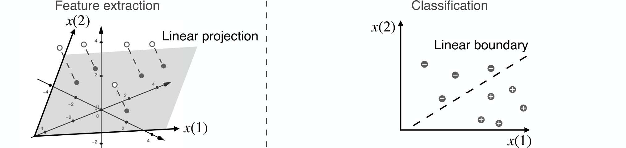

II-C1 Linear Classification Model
Consider the progressive transmission of an arbitrary feature vector and let denote the -th feature (coefficient). Let denote the cumulative index set of features received by the server by the end of slot , where . The corresponding partial feature vector, denoted as , can be defined by setting its coefficients as
| (2) |
In each slot, the server estimates the label of the object by inputting the partial vector into a classifier. We consider two classification models as described in the sequel.
The maximum likelihood (ML) classifier for the distribution (1) is a linear one [18], and relies on a classification boundary between a class pair being a hyper-plane in the feature space (see Fig. 2(a)). Due to uniform prior on the object classes, the ML classifier is equivalent to a maximum a posterior (MAP) classifier and the estimated label is obtained as
| (3) |
where denotes the -th diagonal entry of the covariance matrix . The Mahalanobis distance refers to the distance from the sample to the centroid of class- in the -dimensional feature subspace. Given the ground-truth label for being , let denote the half squared Mahalanobis distance: . Then the problem of linear classification reduces to one of Mahalanobis distance minimization: .
II-C2 CNN Classification Model
A CNN model comprises multiple convolutional (CONV) layers followed by multiple fully-connected (FC) layers. To implement split inference, the model is divided into device and server sub-models as shown in Fig. 2 (b), which are represented by functions and , respectively. Following existing designs in [14, 13], the splitting point is chosen right after a CONV layer. Let denote the number of CONV filters in the last layer of , each of which outputs a feature map with height and width . The tensor of all extracted feature maps from an arbitrary input sample is denoted as , and the -th map as . Let denote the tensor of cumulative feature maps received by the server by slot , and the corresponding index set of feature maps. Then can be related to as
| (4) |
We define the system state for this generic model as . In slot , the server sub-model can compute the posteriors for the input using the forward-propagation algorithm [3]. Then, the label is estimated by posterior maximization: .
II-D Classification Metrics
For the tractable case of linear classification, relevant metrics are characterized as follows.
II-D1 Inference Uncertainty
II-D2 Discriminant Gain
Pairwise discriminant gain measures the discernibility between two classes in a subspace of the feature space. We adopt the well known metric of symmetric Kullback-Leibler (KL) divergence defined as follows [16]. To this end, consider a class pair, say class and , and a feature subspace spanning the dimensions indexed by the set . Let denote the corresponding pairwise discriminant gain. Based on the discussed data distribution model, the feature vector in this subspace is a uniform mixture of Gaussian components with mean and covariance matrix (), where and
| (6) |
Based on the metric of symmetric KL divergence, pairwise discriminant gain is evaluated as,
| (7) |
where . The term is named the pairwise discriminant gain in dimension-. We define the average discriminant gain over all class pairs as
| (8) |
where is the average discriminant gain of dimension-. We refer to (8) as the additivity of discriminant gains. For binary classification, the subscripts of and are omitted for simplicity, yielding and .
III ProgressFTX Protocol and Control Problem
III-A ProgressFTX Protocol

The ProgressFTX protocol implements a time window of continuous progressive feature transmission of a single data sample. If the remote inference fails to achieve the target accuracy, the task is declared a failure for a latency sensitive application (e.g., autonomous driving) or otherwise another instance of progressive transmission may be attempted after some random delay. The steps in the ProgressFTX protocol are illustrated in Fig. 3 and described as follows.
- 1.
Feature selection: At the beginning of a slot intended for feature transmission, the server selects the feature dimensions and informs the device to transmit corresponding features. For the case of linear classification, feature selection uses the importance metric of discriminant gain (see Section II-D); for the other case of CNN classification, the selection of feature maps depend on their importance levels (i.e., descent gradients as elaborated in Section VI-A) which are available from the training phase and to be used in the ensuing phase of edge inference. Two facts should be emphasized: 1) both methods are data-sample independent, which facilitates efficient implementation at the server since it has no access to samples; and 2) feature importance is evaluated using a trained model, but not during the training. Specifically, the server records received features in and their indices in . The indices of selected features are stored in , where . A subset satisfying this constraint is termed an admissible subset. Moreover, the number of features to be transmitted, , is limited by the number of untransmitted features and the transmission rate: .
- 2.
Stopping control: The number of features of a particular sample needed for remote classification to meet the accuracy requirement is sample dependent (for both linear and CNN classifications). Neither the device nor the server has prior knowledge of this number since each has access to either the sample or the model but not both. Online stopping control aims at minimizing the number of transmitted features under the said requirement. Its procedure is described as follows while its optimization problem is formulated in Section III-B and solved in Section V. Let indicate the server’s decision on whether the device should transmit features in slot (i.e., ), or stop the progressive transmission (i.e., ). The decision is made using a derived policy for the case of linear classification (see Section V) or a regression model for uncertainty prediction (see Section VI-B). If the decision is to transmit, proceed to the next step; otherwise, go to Step .
- 3.
Feedback: The decisions on feature selection and stopping control are communicated to the device by feedback of one of three available control signals described as follows: (a) If the channel is not in outage in the preceding slot, the feedback contains a transmit-new-features signal and indices of features in that instructs the device to transmit the features selected by the server in the current slot. (b) Otherwise, the feedback is a retransmission signal instructing the device to retransmit the features transmitted in the preceding slot. In this case, a link-layer HARQ protocol is employed to enable retransmission. (c) If the server decides to stop the transmission (i.e., ), a stop signal is fed back to instruct the device to terminate feature transmission.
- 4.
Feature transmission: Upon receiving a transmit-new-features signal with indices , the device transmits the incremental feature vector, , that comprises the selected features:
(9) where are indices in . At the end of slot-, the server updates the set of received features and the partial feature vector , where the entry in the -th row and -th column of the placement matrix is
(10) - 5.
Server inference: The server infers an estimated label and its uncertainty level using the partial feature vector and a trained model as discussed in Section II-C. Then we go to Step 1 and restart ProgressFTX for another data sample.
- 6.
Termination: Upon receiving a stop signal, the device terminates the process of progressive transmission. The latest estimated label is downloaded to the device.
In summary, feature selection, stopping control, feature transmission and uncertainty evaluation are executed sequentially in each slot. The transmission is terminated at the time when the uncertainty is evaluated to fall below the target or uncertainty reduction is outweighed by the corresponding communication cost.
III-B Control Problem Formulation
ProgressFTX has two objectives: 1) maximize the uncertainty reduction (or equivalently, improvement in inference accuracy), and 2) minimize the communication cost. The optimal stochastic control is formulated as a dynamic programming problem as follows. We define the system state observed by the server at the beginning of slot as the following tuple
| (11) |
Recall that represents the transmission rate in slot , the received partial feature vector, and the indices of received features. The control policy, denoted as , maps to the feature-selection action, , and stopping-control action, , . The net reward of transitioning from to is the decrease in inference uncertainty minus the communication cost, which can be written as
| (12) |
where denotes the transmission cost of one slot. For sanity check, if . The net reward for slot requires server’s evaluation based on transmitted features if the control decision is proceeding transmission or retransmisson; and thus, is unknown before making the decision for the slot. Hence, the expected net reward should be considered as the utility function. Without loss of generality, consider slots with the current slot set as slot . Then the system utility is defined as the expectation of the sum rewards over slots conditioned on the system state and control policy:
| (13) |
The ProgressFTX control problem can be readily formulated as the following dynamic program:
The complexity of solving the problem using a conventional iterative algorithm (e.g., value iteration) is prohibitive due to the curse of dimensionality as the state space in (13) is not only high dimensional but also partially continuous. The difficulty is overcome in the sequel via analyzing the structure of the optimal policy.
IV ProgressFTX Control – Optimal Feature Selection
In this section, targeting linear classification, the optimal policy for feature selection in the ProgressFTX protocol is derived in closed form by first approximating the objective function in Problem (P1), and then solving the problem.
IV-A Approximation of Expected Uncertainty
IV-A1 Binary Classification
For ease of exposition, we first consider the simplest case of binary classification (i.e., ) before extending the results to the general case. The goal of the subsequent analysis is to approximate the expected uncertainty function of unknown features to be transmitted in the following slots, given the features already received by the server, which is the objective of Problem (P1) in (13). To begin with, the objective can be rewritten as
Based on the fact that feature distributions in different dimensions are independent (as the covariance matrix is diagonal), telescoping gives
| (14) |
In the remainder of the sub-section, we show that the expected uncertainty term in can be reasonably approximated by a monotone decreasing function of the average discriminant gain of selected features, which facilitates the subsequent feature-selection optimization.
Consider first the feature-selection decisions for transmission over slots specified by . Upon receiving the selected features , the partial feature vector is updated as , where the placement matrix , defined similarly as in (10), places all the features transmitted over slots as recorded in . For an arbitrary feature vector , define the differential-distance as , where and represent the half squared Mahalanobis distances from to the centroids of classes and , respectively. For ease of notation, let and be denoted as and , respectively. In particular,
| (15) |
Note that is a random variable from the server’s perspective before receiving the selected features. Given the GM model (1), the distribution of is characterized next.
Lemma 1.
Given the partial feature vector and feature-selection decision , the differential distance is a mixture of two Gaussian components with the following conditional PDF:
| (16) |
where is the total discriminant gain of features selected in given in (7).
Given a differential distance , the inference uncertainty in (5) can be simplified as:
| (17) |
Then the expected uncertainty resulting from the feature-selection decision can be written as
| (18) |
In view of the difficulty in deriving the above integral in closed form, we resort to its approximation using an upper bound as shown in the following lemmas.
Lemma 2.
Given , the inference uncertainty can be upper bounded by
| (19) |
Proof.
The result follows from the fact that the ratio has the maximum value of , which is smaller than one, at . ∎
For large , the bound is tight since . Using Lemma 2, we can bound the expected uncertainty as with
| (20) |
where is given in Lemma 2. The above analysis allows approximating by a simple exponential upper bound as shown in Lemma 3, proven in Appendix A. This approximation is also validated numerically in Fig. 4.
Lemma 3.
The expected uncertainty can be upper bounded by an exponential function as
| (21) |
where and are positive constants depending on .
IV-A2 Extension to Multi-class Classification
The above analysis for binary classification can be generalized for multi-class classification (i.e., ) as follows. The inference uncertainty in the case of multi-class classification can be upper bounded in terms of pairwise uncertainties,
where and the equality is approached in the asymptotic case that there exists an infinitely small compared with other pairwise differential distances. Moreover, the distribution of conditioned on a partial feature vector and a feature-selection decision is a mixture of scalar Gaussian components, similar to its counterpart in binary classification (16). As a result, an upper bound on the conditional expected inference uncertainty can be obtained following the approach for binary classification, i.e., substituting with as that in (20). Given the above straightforward procedure, the remainder of the paper assumes binary classification to simplify notation and exposition.
IV-B Optimal Feature Selection
First, Problem (P1) reduces to the problem of optimal feature selection by conditioning on subsequent transmissions, i.e., transmission is stopped at slot . The decision can be captured by defining a sequence of virtual transmission rates such that for and , while otherwise. Moreover, approximate the function in the objective in Problem (P1) by its upper bound in Lemma 3. Given the stopping decision and approximate objective, Problem (P1) reduces to the following problem.
It follows from the monotonicity of the objective that the optimal policy for feature selection in each slot is to choose from not yet received features whose indices correspond to the maximum discriminant gains. Let the importance of each feature be associated with its discriminant gain. Then the optimal policy, termed importance-aware feature selection, is as presented in Algorithm 1.
1: Feature selection for one slot.
for do
Select the most important feature from the admissible set , and add the selected feature index to , i.e., ;
end for 2: Update. Update the set of virtually received features’ indices as ;
Output: .
V ProgressFTX Control – Optimal Stopping
Given the importance-aware feature selection process in the preceding section, we describe the remaining design of ProgressFTX to solve the problem of optimal stopping control. Following the notation used in Section IV-B, transmission is assumed to stop in slot , resulting in transmitted incremental feature vectors. The stopping-control indicators and can be related as
| (22) |
As before, for tractability, we approximate the objective in Problem (P1) (see (14)) using the upper bound in Lemma 3. Then given the optimally selected and transmitted features , Problem (P1) can be approximated as
Note the dependence of the equivalent optimal feature selection on the random channel gain . Problem (P3) belongs to the class of optimal-stopping problems [22]. In operation, the server makes a binary decision (i.e., or ) on whether to transmit in the current slot. The solution for Problem (P3) can be converted into the control decision, , by
| (23) |
The optimal control policy (also known as optimal stopping-rules) are derived for both the Gaussian and fading channels in the following subsections.
V-A Optimal Stopping with Gaussian Channels
In this subsection, we address the optimal stopping for Gaussian channels, where . In this case, the optimal feature subsets for all current and future slots can be determined by the importance aware feature selection (i.e., Algorithm 1) at the beginning of the current slot. Given the total throughput in proceeding transmissions, , the total number of features selected for transmission is where specifies the number of untransmitted features in the current slot. Let denote the discriminant gain of optimally selected features subject to a number of transmissions and conditioned on . Then the cumulative discriminant gain over transmissions is obtained as . Problem (P3) can be rewritten for a Gaussian channel as
This problem is convex. To prove this, we first rewrite the cumulative discriminant gain as
| (24) |
Using the fact that for all , one can infer from the last equation that
| (25) |
and thereby conclude that is concave with respect to (w.r.t.) . Combining this fact and that is a convex and monotone decreasing function of shows that Problem (P4) is also convex. Based on a standard approach in discrete convex optimization [23], the optimal solution for Problem (P4) can be derived as
| (26) |
where is given by
| (27) |
Combining (23), (26), and (27) leads to the following main result of the section.
Theorem 1 (Optimal Stopping for Gaussian Channels).
The stopping rule for Gaussian channels, which solves Problem (P4), is that the transmission in ProgressFTX should be terminated if . In other words, the optimal stopping policy is given as
| (28) |
where the incremental reward (i.e., reduction in classification uncertainty) from transmission in the current slot is denoted as .
The optimal stopping policy in Theorem 1 is interpreted as follows. As grows, the transmission cost accumulates at a constant speed , while the incremental reward from transmission in slot monotonically decreases due to the convexity of the function (see Lemma 3 and (25)). For this reason, is exactly the maximum number of subsequent transmissions such that the incremental reward from transmitting in slot is no larger than the per-slot transmission cost, yielding the stopping threshold. In the special case of , transmissions should be terminated in the current slot.
The server algorithm for controlling ProgressFTX, including both feature selection and optimal stopping, is summarized in Algorithm 2, where the index refers to the -th slot in an edge inference task instead of that for slot from a current slot in control problems.
1: Feature selection. Determine optimal feature subset by Algorithm 1; 2: Stopping control. Evaluate the optimal stopping control indicator by (28); 3: if then:
1) Feature transmission. Receive the incremental feature vector ; 2) Partial feature vector update. Update the partial feature vector by the rule , with the placement matrix given by (10); 3) System state evolution. Evolve to state ;
V-B Optimal Stopping with Fading Channels
In this sub-section, the optimal stopping policy for Gaussian channels is extended to the case of fading channels with outage. This requires that two issues be addressed. The first is the optimal retransmission strategy upon the occurrence of an outage event. Given importance-aware feature selection, the features that fail to be received due to channel outage are most important ones among the undelivered features. This leads to the following strategy.
Lemma 4 (Optimality of Feature Retransmission).
To minimize classification uncertainty, it is optimal to retransmit an incremental feature vector, whose transmission fails due to channel outage, in the next slot.
The second issue is whether the optimal stopping problem in the current case retains the convexity of its Gaussian-channel counterpart. The answer is positive as shown in the sequel. Given the fixed communication rate and channel outage probability , the transmitted features can be successfully received with probability . The number of successful transmissions out of trials, denoted by , follows a Binomial distribution, . The conditional probability mass function (PMF) of is given by
| (29) |
Based on the retransmission strategy in Lemma 4, the total discriminant gain of features in successfully received incremental feature vectors is given by defined in (24). Combining and (29), the expectation of the upper bound of uncertainty after times of transmission is denoted as and given by
| (30) |
Then Problem (P3) can be rewritten for a fading channel with outage as
Lemma 5.
The problem of optimal stopping for a fading channel with outage, namely Problem (P5), is convex.
Proof.
See Appendix -B. ∎
Given the convexity and following the arguments used to solve Problem (P4), the optimal solution for Problem (P5) is derived to be
| (31) |
where in this case is given by
| (32) |
The optimal stopping rule follows from (23), (31), and (32), leading to the following:
Theorem 2 (Optimal Stopping for Fading Channels).
The stopping rule for a fading channel with outage, which solves Problem (P5), is that the transmission in ProgressFTX should be terminated if . The corresponding optimal stopping policy is given as
| (33) |
where the incremental reward follows that in Theorem 1.
Comparing Theorems 1 and 2, the optimal stopping policy in the case of fading channel retains the threshold based structure of its Gaussian-channel counterpart. Nevertheless, the transmission threshold is higher in the former than that in the latter (by a factor of ) due to the additional communication cost caused by channel outage. To be specific, given the same level of uncertainty reduction, the needed number of transmission, say , in the case of Gaussian channel is expected to increase to when fading is present. As a result, a requirement on inference accuracy achievable in the Gaussian channel case may not be affordable in the fading channel case.
ProgressFTX control in Algorithm 2 can be easily modified to account for outage in fading channels as follows. First, the optimal stopping control indicator shall be evaluated by (33) instead. Next, Step 3 should be modified as follows. If the transmission in sub-step 1) is successful, then sub-step 2) is partial feature vector update as presented in Algorithm 2; otherwise, sub-step 2) involves the server sending a retransmission signal to the device for retransmission.
VI ProgressFTX for CNN Classifiers
Given the complex architecture of a CNN model, ProgressFTX for a CNN classifier cannot be directly designed using an optimization approach as in the preceding sections for its linear counterpart. To overcome the difficulty, we leverage the principles underpinning the optimized ProgressFTX policies, namely importance-aware feature selection and optimal stopping, for the linear model to design their counterparts under the CNN model as follows.
VI-A Importance-aware Feature Selection
Consider the step of feature selection in the ProgressFTX protocol in Section III-A. The discriminant gain defined in (7) for a linear classifier, which underpins the associated metric of feature importance, is not applicable to a CNN model. In this case, we propose the use of another suitable metric proposed in [15], which is introduced next. Consider the parameters of the last CONV layer of the device sub-model. Let denote the -th entry of the gradient, i.e., the partial derivative of the learning loss function w.r.t. the parameter , which is available from the last round of model training as computed using the back-propagation algorithm. Then its importance can be measured using the associated reduction of learning loss from retaining , approximated by the following first-order Taylor expansion of the squared loss of prediction errors [15]: . The importance of the -th feature map is defined to be the summed importance of parameters in the -th filter outputting the map: . Since are readily available in training, the server is able to obtain the value of after training and form a lookup table for reference during ProgressFTX control. Given , the importance-aware feature selection for each slot is performed by selecting a given number of most important filters, whose feature maps will be transmitted in the slot. It should be reiterated that the number of selected feature maps is communication-rate dependent and may varies over slots. Algorithm 1 for the linear classifier can be modified accordingly. The details are straightforward, and thus omitted.
VI-B Stopping Control Based on Uncertainty Prediction
Consider the step of stopping control in the ProgressFTX protocol in Section III-A. The optimal stopping control in the current case is stymied by the difficulty in finding a tractable and accurate approximation of the expected classification uncertainty as a function of input features similarly to Lemma 3 for linear classification. To tackle the challenge, we resort to an algorithmic approach in which a regression model is trained to predict the uncertainty function of feature maps to be transmitted in the following slots given the feature maps already received by the server. One particular popular architecture of regression models in the literature is adopted [24, 25]. To be able to predict the uncertainty for a future partial feature-map tensor, both the current partial feature-map tensor and the selected index subset are needed as the input. Since the underpinning prediction is based on the current partial feature maps, ProgressFTX control for CNN models is also sample-dependent. The architecture contains concatenation of two streams of regression features extracted from the feature-map tensor, , and the index subset , into one intermediate feature map, fed into the deeper layers of the regression model (see Fig. 5).
To train the regression model, a training dataset and a prediction loss function need to be properly designed. The training dataset on the server, denoted as , comprises labeled samples , each with the a tuple of and a scalar label , . Consider a tensor of all feature maps extracted by the server sub-model from an arbitrary sample and denoted by . The first entry in , , is a tensor of arbitrary partial feature maps drawn from , which represent the feature maps already received by the server. The second entry is an admissible subset of indexes representing feature maps to be transmitted (hence not in ). Then the label is the exact inference uncertainty generated by the server sub-model for the input of a tensor comprising both feature maps in and the feature maps indexed in drawn from , i.e., . Next, to train the prediction model, the loss function is designed to be the mean-square error between the predicted result and the ground-truth. A stochastic gradient descent (SGD) optimizer is adopted to train the model, denoted as with parameters , by minimizing the loss function:
| (34) |
Given the current state and the trained inference uncertainty predictor , the online stopping control problem is written as
| (35) |
The optimal stopping time from the current slot, namely , can be determined by linear search. Then the stopping decision in the current slot is . Even for a Gaussian channel, the number of transmission slots for different samples differ due to their requirements of feeding different numbers of features into classifier to reach the same target confidence level if it is possible.

VII Experimental Results
VII-A Experimental Settings
The experimental setups are designed as follows, unless specified otherwise. Each feature is quantized at a high resolution, bits/feature, for digital transmission. The horizon in online scheduling is set as slots. A statistical (GM) dataset is used for training and testing the linear model and the popular MNIST dataset of handwritten digits for the CNN model. The settings in the two cases are described as follows. Consider the case of linear classification. For the GM dataset, there are classes with features in total for each sample. Due to the small number of features, only a narrow-band channel is needed whose bandwidth is set as kHz. The slot duration is milliseconds. For the case of Gaussian channel, the channel SNR is set as dB such that the transmission rate is features/slot. For the case of fading channel, the transmit rate is fixed at features/slot while the outage probability is . For the case of CNN, we use the well-known LeNet [15]. The Gaussian channel in this case has a bandwidth of MHz, the slot duration of milliseconds, and the channel SNR dB. The corresponding transmission rate is feature-maps/slot.
The optimal control of ProgressFTX in the case of CNN classification requires an uncertainty predictor as designed in Section VI. Its architecture comprises two input layers, as illustrated in Fig. 5. The first one reshapes an input tensor for partial feature maps into a vector. The second one reshapes the feature selection input into a vector, where the coefficient is if the corresponding feature map index is selected or otherwise. These two vectors are concatenated and then fed into three fully-connected layers with , , and neurons, respectively. There is one neuron in the last output layer providing a prediction of uncertainty. The test mean-square error of the uncertainty predictor trained for epochs is low to .
Two benchmarking schemes are considered. The first scheme, termed one-shot compression, uses the classic approach of model compression: given importance-aware feature selection, the number of features to transmit, , is determined prior to transmission such that it meets an uncertainty requirement The value of is solved from for linear classifiers or for CNN classifiers, respectively. The drawback of this scheme is that its lack of ACK/NACK feedback as for ProgressFTX makes the device inept in minimizing the number of features to achieve an exact uncertainty level. In the current experiments, the device has to instead target the expected uncertainty approximated in (21) for the case of linear classification or predict the uncertainty in the case of CNN classification. The second scheme, termed random-feature optimal stopping, modifies the optimal ProgressFTX by removing feature importance awareness and instead selecting features randomly.
VII-B Linear Classification Case
First, we evaluate the effect of importance-aware feature selection on inference performance. To this end, discriminant gains of different feature dimensions, which are arranged in a decreasing order, are plotted in Fig. 6(a). In Fig. 6(b), the levels of inference accuracy and uncertainty are plotted against the number of received features arranged in the same order. One can observe the monotonic reduction of accuracy and growth of uncertainty as the number of features increases. The result confirms the usefulness of importance awareness in feature selection for shortening the communication duration given target inference accuracy (or expected uncertainty).
Define the average communication latency of a transmission scheme for edge inference as the average number of transmission slots required for meeting a requirement on inference accuracy or expected uncertainty. Considering a Gaussian channel, the average communication latency of ProgressFTX and two benchmarking schemes are compared for varying target accuracy and expected uncertainty in Fig. 7. As observed from the figures, the proposed ProgressFTX technique achieves the lowest latency based on both the criteria of achieving targeted uncertainty and accuracy. For instance, two benchmarking schemes require in average slots to achieve an accuracy of while ProgressFTX only requires . In terms of uncertainty, in average slots are used to achieve uncertainty of for ProgressFTX. In comparison, the average latency for one-shot compression and random-feature optimal stopping are about and higher, respectively. Moreover, ProgressFTX achieves the lowest average inference uncertainty of and the highest accuracy of . The average communication latency of the three schemes are also compared in the case of a fading channel in Fig. 8. In the presence of fading, ProgressFTX continues to outperform benchmarking schemes. The above comparisons demonstrate the gains of importance awareness in feature selection and optimal stochastic control of transmission.
Define the transmission probability of a feature dimension as the fraction of samples whose inference requires the transmission of the feature in this dimension. To further compare ProgressFTX with benchmarking schemes, the curves of transmission probability of each feature dimension versus its importance level (i.e., discriminant gain) are plotted in Fig. 9 for the case of linear classification and Gaussian channel. One can observe that the transmission probability is almost uniform over unpruned feature dimensions for the scheme of one-shot compression and all dimensions for the scheme of random-feature optimal stopping. This indicates their lack of feature importance awareness. In contrast, the probabilities for ProgressFTX are highly skew with higher probabilities for more important feature dimensions and vice versa. The skewness arises from the importance-aware feature selection as well as the stochastic control of transmissions which are the key reasons for the performance gain of ProgressFTX over the benchmark schemes.
VII-C CNN Classification Case
We consider the case of CNN classification where ProgressFTX is controlled using the algorithms developed in Section VI. To implement split inference, the split point of LeNet is chosen to be right after the second CONV layer in the model. As a result, the device can choose from feature maps for transmission to the server. To rein in the complexity of model architecture and training, we consider a Gaussian channel as commonly assumed in the literature (see e.g., [5, 9]). Given these settings, one sample per inference task and feature maps transmitted in one slot, at most slots are required to transmit all maps.
First, the curves of inference performance (i.e., inference accuracy and uncertainty) versus the number of transmitted feature maps, selected with importance awareness, are plotted in Fig. 10. The tradeo-ffs are similar to those in the linear-classification case in Fig. 6(b). Particularly, due to importance-aware feature selection, the accuracy is observed to rapidly grow and the uncertainty quickly reduces as the number of received feature maps increases.
The comparisons in Fig. 7 is repeated in Fig. 11 for the CNN classifier. The same observation can be made that ProgressFTX outperforms the benchmark schemes over the considered ranges of inference uncertainty and accuracy. For instance, given transmission slots in average, ProgressFTX achieves the uncertainty of and accuracy of which are at least lower and higher than the benchmarking schemes. As another example, for the target accuracy of , one can observe from Fig. 11(b) that ProgressFTX requires in average slots while one-shot compression requires , corresponding to latency reduction for the former. Last, the transmission probabilities of different feature maps are plotted against their importance levels in Fig. 12. The observations are similar to those for the linear model in Fig. 9.
VIII Concluding Remarks
In this paper, a novel feature transmission technique termed ProgressFTX has been proposed for communication-efficient edge inference. ProgressFTX progressively selects and transmits important features until the desired inference performance level is reached, or terminates the transmission judiciously to improve the inference performance while reducing the transmission cost. Comprehensive experimental results demonstrate its benefits in reducing the communication latency under given inference performance targets. This first study of ProgressFTX opens a new direction to edge inference. A series of interesting topics for further study are warranted, such as power control and device scheduling for multi-device ProgressFTX.
-A Proof of Lemma 3
Substituting (16) and (19) into (20), one can observe that the targeted integral consists of a group of integrals of Gaussian and exponential functions. This kind of integral is well-known in the literature that not to tend itself for a closed-form expression but can be expressed in terms of multiple complementary error functions [26, 27]. Due to limited space, we do not present the expression of but directly report a fact derived from the expression, . This results in , where is the Bachmann–Landau notation establishing equivalence between shrinking rates of two functions. Consequently, given any , monotonically decays to zero at a super-exponential rate in the asymptotic regime of . This scaling law proofs Lemma 3.
-B Proof of Convexity of Problem (P5)
To show the convexity of Problem (P5), it is equivalent to prove the following inequality holds for , that is where is the second-order difference of w.r.t. its second argument. To begin with, we construct a function defined as where is an arbitrary linear function with constants and . The closed-form expression of is evaluated to be . Consequently, the second-order difference of w.r.t. always equals to zero, i.e.,
| (36) |
The analytical form of the second-order difference of PMF w.r.t. , which is denoted as , is given by
| (37) | |||||
Observes from (37) that the sign of is determined by , a convex quadrature function of . Specifically, and hold. We conclude that given , is non-positive only in one closed integral of consecutive integers , where the left and right end-points are denoted by and , respectively.
We expand and as and respectively. Choose and such that if and if . Due to , one can conclude that
| (38) |
Next, we note that is strictly convex and monotonically decreasing w.r.t. while is linear. It is always able to find an with sufficiently small such that
| (39) |
Combining (36), (38) and (39) leads to the desired results, which completes the proof.
| (40) |
References
- [1] M. Chen, D. Gündüz, K. Huang, W. Saad, M. Bennis, A. V. Feljan, and H. V. Poor, “Distributed learning in wireless networks: Recent progress and future challenges,” [Online] https://arxiv.org/pdf/2104.02151.pdf, 2021.
- [2] G. Zhu, D. Liu, Y. Du, C. You, J. Zhang, and K. Huang, “Toward an intelligent edge: Wireless communication meets machine learning,” IEEE Commun. Mag., vol. 58, no. 1, pp. 19–25, 2020.
- [3] X. Wang, Y. Han, V. C. M. Leung, D. Niyato, X. Yan, and X. Chen, “Convergence of edge computing and deep learning: A comprehensive survey,” IEEE Commun. Surv. Tut., vol. 22, no. 2, pp. 869–904, 2020.
- [4] X. Huang and S. Zhou, “Dynamic compression ratio selection for edge inference systems with hard deadlines,” IEEE Internet Things J., vol. 7, no. 9, pp. 8800–8810, 2020.
- [5] W. Shi, Y. Hou, S. Zhou, Z. Niu, Y. Zhang, and L. Geng, “Improving device-edge cooperative inference of deep learning via 2-step pruning,” in Proc. IEEE INFOCOM Workshops, Paris, France, Apr. 29 - May 2, 2019.
- [6] E. Li, L. Zeng, Z. Zhou, and X. Chen, “Edge AI: On-demand accelerating deep neural network inference via edge computing,” IEEE Trans. Wireless Commun., vol. 19, no. 1, pp. 447–457, 2020.
- [7] J. Shao and J. Zhang, “Communication-computation trade-off in resource-constrained edge inference,” IEEE Commun. Mag., vol. 58, no. 12, pp. 20–26, 2020.
- [8] J. Shao and J. Zhang, “Bottlenet++: An end-to-end approach for feature compression in device-edge co-inference systems,” in Proc. IEEE Int. Conf. Commun. Workshops (ICC WKSHPS), Dublin, Ireland, Jun. 7-11, 2020.
- [9] M. Jankowski, D. Gündüz, and K. Mikolajczyk, “Joint device-edge inference over wireless links with pruning,” in Proc. IEEE Int. Workshop Signal Process. Adv. Wireless Commun. (SPAWC), Atlanta, GA, USA, May 26-29, 2020.
- [10] M. Jankowski, D. Gündüz, and K. Mikolajczyk, “Wireless image retrieval at the edge,” IEEE J. Sel. Areas Commun., vol. 39, no. 1, pp. 89–100, 2021.
- [11] X. Xu, Y. Ding, S. X. Hu, M. Niemier, J. Cong, Y. Hu, and Y. Shi, “Scaling for edge inference of deep neural networks,” Nature Electron., vol. 1, no. 4, pp. 216–222, 2018.
- [12] C. Szegedy, W. Liu, Y. Jia, P. Sermanet, S. Reed, D. Anguelov, D. Erhan, V. Vanhoucke, and A. Rabinovich, “Going deeper with convolutions,” in Proc. IEEE Conf. Comput. Vision Pattern Recog. (CVPR), Boston, MA, USA, Jun. 7-12, 2015.
- [13] J. Guo, W. Ouyang, and D. Xu, “Channel pruning guided by classification loss and feature importance,” in Proc. AAAI Conf. Artificial Intell. (AAAI), New York, NY, USA, Feb. 7-11, 2020.
- [14] Z. Zhuang, M. Tan, B. Zhuang, J. Liu, Y. Guo, Q. Wu, J. Huang, and J. Zhu, “Discrimination-aware channel pruning for deep neural networks,” in Proc. Adv. Neural Inf. Process. Syst. (NeurIPS), Montreal, Canada, Dec. 3-8, 2018.
- [15] P. Molchanov, A. Mallya, S. Tyree, I. Frosio, and J. Kautz, “Importance estimation for neural network pruning,” in Proc. IEEE/CVF Conf. Comput. Vision Pattern Recogn. (CVPR), Long Beach, CA, USA, Jun. 16-20, 2019.
- [16] G. Saon and M. Padmanabhan, “Minimum bayes error feature selection for continuous speech recognition,” in Proc. Adv. Neural Inf. Process. Syst. (NeurIPS), Denver, CO, USA, Jan. 1, 2000.
- [17] S. Lin and P. Yu, “A hybrid ARQ scheme with parity retransmission for error control of satellite channels,” IEEE Trans. Commun., vol. 30, no. 7, pp. 1701–1719, 1982.
- [18] T. Hastie, R. Tibshirani, and J. Friedman, The Elements of Statistical Learning: Data mining, Inference, and Prediction. New York, NY, USA: Springer Science & Business Media, 2009.
- [19] S. Weber, X. Yang, J. Andrews, and G. de Veciana, “Transmission capacity of wireless ad hoc networks with outage constraints,” IEEE Trans. Inf. Theory, vol. 51, no. 12, pp. 4091–4102, 2005.
- [20] D. Liu, G. Zhu, Q. Zeng, J. Zhang, and K. Huang, “Wireless data acquisition for edge learning: Data-importance aware retransmission,” IEEE Trans. Wireless Commun., vol. 20, no. 1, pp. 406–420, 2021.
- [21] D. Liu, G. Zhu, J. Zhang, and K. Huang, “Data-importance aware user scheduling for communication-efficient edge machine learning,” IEEE Trans. Cogn. Commun. Netw., vol. 7, no. 1, pp. 265–278, 2021.
- [22] Y. Chow, H. Robbins, and D. Siegmund, Great expectations: The theory of optimal stopping. Boston, MA, USA: Houghton Mifflin, 1971.
- [23] K. Murota, “Discrete convex analysis,” Math. Program., vol. 83, no. 1, pp. 313–371, 1998.
- [24] D. F. Specht, “A general regression neural network,” IEEE Trans. Neural Netw., vol. 2, no. 6, pp. 568–576, 1991.
- [25] J. Gao, Q. Wang, and Y. Yuan, “SCAR: Spatial-/channel-wise attention regression networks for crowd counting,” Neurocomputing, vol. 363, pp. 1–8, 2019.
- [26] O. Olabiyi and A. Annamalai, “Invertible exponential-type approximations for the Gaussian probability integral Q(x) with applications,” IEEE Wireless Commun. Lett., vol. 1, no. 5, pp. 544–547, 2012.
- [27] M. Chiani, D. Dardari, and M. Simon, “New exponential bounds and approximations for the computation of error probability in fading channels,” IEEE Tran. Wireless Commun., vol. 2, no. 4, pp. 840–845, 2003.