Simple Coding Techniques
for Many-Hop Relaying

We consider a chain of $m+1$ nodes indexed by $\{0,1,\dotsc,m\}$; node $0$ is the encoder, node $m$ is the decoder, and the remaining nodes are relays. Node $0$ is given a binary random variable $\Theta$ that takes a value in $\{0,1\}$, each with probability $\frac{1}{2}$. At each time step $i\in\{1,2,\ldots,n\}$, node $j$ ($0\leq j\leq m-1$) sends one bit $X_{i,j}$ to node $j+1$ through a binary symmetric channel (BSC) with crossover probability $p\in\big(0,\frac{1}{2}\big)$; we denote the output of this transmission by $Y_{i,j}$. The channels are assumed to be memoryless and independent across nodes. Importantly, $X_{i,j}$ can only depend on what was previously received, i.e., $Y_{1,j-1},Y_{2,j-1},\ldots,Y_{i-1,j-1}$. After $n$ time steps, node $m$ outputs an estimate $\hat{\Theta}$ of $\Theta$.

For a given number of nodes $m$ and BSC crossover probability $p$, let $n^{*}(m,p)$ be the minimum block length $n$ for which there exists a protocol (encoding, relaying, and decoding) such that $\mathbb{P}(\hat{\Theta}\neq\Theta)\leq\frac{1}{3}$.¹¹ 1 Any other fixed constant in $\big(0,\frac{1}{2}\big)$ could also be used, or one could require that $\mathbb{P}(\hat{\Theta}\neq\Theta)\to 0$ as $m\to\infty$; our results will handle all of these variants. The information velocity is defined as follows:²² 2 We are not aware of a formal proof that this limit always exists. However, all of our results will remain valid regardless of whether the $\liminf$ or $\limsup$ is used in place of the regular limit.

We note that $v(0)=1$, and $v(p)\in[0,1]$ for all $p$. Analogously, we say that a protocol (or more precisely, a sequence of protocols indexed by $m$) attains positive information velocity if³³ 3 Throughout the paper, we use the standard asymptotic notation $\mathcal{O}(\cdot)$, $\Omega(\cdot)$, $\Theta(\cdot)$, $o(\cdot)$, and $\omega(\cdot)$. The distinction between asymptotic $\Theta(\cdot)$ notation and the unknown bit $\Theta\in\{0,1\}$ will be clear from the context, as well as the presence/absence of brackets. $n=\mathcal{O}(m)$ and the error probability is at most $\frac{1}{3}$ for all sufficiently large $m$. We will also be interested in the possible decay rate of the error probability towards zero.

Contributions. In this paper, we present a simple, efficient, and deterministic protocol attaining positive information velocity (see Theorem 1 and Corollary 1 below), based on the idea of having different nodes estimate $\Theta$ by processing bit sequences of different lengths (e.g., most nodes process 1 or 3 bits at a time, but a small minority of nodes consider blocks of size $\omega(1)$ or even $\mathcal{O}(m)$) and using a recursive decoding technique. In addition, we characterize the asymptotic behavior of $v(p)$ in the limits $p\to 0$ and $p\to\frac{1}{2}$, showing that $v(p)=1-\Theta(p)$ as $p\to 0$, and $v\big(\frac{1-\delta}{2}\big)=\Theta(\delta^{2})$ as $\delta\to 0$. Finally, we provide a multi-bit generalization of our protocol that can reliably transmit $\mathcal{O}(k)$ bits in $\mathcal{O}(m+k)$ transmissions.

Related work. As noted in [1], the preceding problem was posed at the 2015 Simons Institute program on information theory by Yury Polyanskiy, who also coined the term “information velocity”. At the same workshop, Leonard J. Schulman pointed out an existing solution based on tree codes [2].

In more detail, Rajagopalan and Schulman [2] (building on earlier work by Schulman [3, 4]) studied general techniques for relating noiseless vs. noisy computation in distributed systems using tree codes. An important implication of their main result is that $v(p)>0$, which is obtained by specializing to a chain-structured network. However, the associated computational complexity is exponential, requiring the use of recursive maximum-likelihood decoding. A closed-form upper bound (i.e., converse) on the information velocity can also be inferred directly from [2], which we will strengthen as part of our analysis of the high-noise asymptotics. In the low-noise limit, we find that the converse of [2] already provides tight asymptotic scaling.

A simple and efficient protocol for the setting we consider (and its multi-bit extension) was also proposed in [2], but it falls very narrowly short of attaining positive information velocity, due to requiring $n=\omega(m)$ transmissions; the $\omega(m)$ scaling is extremely mildly super-linear according to the iterated logarithm. This $\omega(m)$ behavior arises from each node waiting to receive $\omega(1)$ useful bits from the previous node before forwarding (see Appendix -A for more details), which our protocol avoids.

A more recent work of Gelles et al. [5] introduces a variant of tree codes that can be decoded in polynomial time. The focus in [5] is on two-way communication channels, but based on [2], it seems feasible that their techniques could be adapted to one-way settings such as the one we consider. On the other hand, such an adaptation would still leave the following relative limitations compared to our approach:

• •

  According to [5, Thm. V.I], when $n=\mathcal{O}(m)$, the error probability can (only) be controlled to be a constant such as $\frac{1}{3}$, whereas our protocol will give stronger $e^{-\Theta(\sqrt{n})}$ decay, and simple variations will further boost this to $e^{-\Theta(n^{1-\epsilon})}$ for any $\epsilon>0$. On the other hand, we still fall short of the $e^{-\Theta(n)}$ decay shown using the inefficient approach of [2].

• •

  The computational complexity in [5] in ${\rm poly}(n)$ with an unspecified power, whereas in our protocol the nodes each incur a computational complexity of $\mathcal{O}(n)$.

• •

  The approach in [5] is randomized, and assumes the availability of common randomness across the nodes, whereas our protocol is deterministic.

Perhaps more important than any of these factors is the fact that that the tree codes of [2, 5] were designed for much more general distributed computation settings, and are accordingly highly versatile but unnecessarily complex for the simpler information velocity problem. In our judgment, the main advantage of our protocol is its simplicity.

A recent work (concurrent with ours) established the exact information velocity of the binary erasure channel (BEC) and other erasure-type channels [6], and also studied the exponential decay rate of the error probability. The protocols therein appear to rely heavily on the property $\Pr[x~{\rm sent}\,|\,x~{\rm received}]=1$ for every non-zero input $x$ (e.g., this holds for the BEC and the Z-channel), which allows information to be propagated with certainty. As a result, handling the BSC with their approach does not appear to be feasible.

Another related line of works studies the optimal error exponent for transmitting one bit over a 2-hop relay network [1, 7, 8]. To our knowledge, none of the coding techniques in these works are suited to attaining positive information velocity. However, we note that the work of Huleihel, Polyanskiy, and Shayevitz [1] highlighted interesting connections between the information velocity problem and the 2-hop setting. In particular, based on the observation that positive information velocity is possible, they conjectured that the 1-hop and 2-hop error exponents should coincide in the high-noise limit so that “information propagation does not slow down”. This conjecture was resolved in the affirmative in our subsequent work [8], where we showed that the 1-hop and 2-hop exponents in fact coincide at any noise level.

Finally, we briefly mention that there exists extensive work on relay channels studying the capacity [9, Ch. 16], error exponent [10], hypothesis testing protocols [11], and so on. We also briefly mention that related many-hop transmission problems were studied for (continuous) channels with input constraints in [12].

We will first describe the protocol assuming $p$ to be sufficiently small (namely, below $\frac{1}{48}$), and then turn to arbitrary $p\in\big(0,\frac{1}{2}\big)$.

The protocol is illustrated in Figure 1, and described in detail as follows. We arrange the nodes into levels. A (relay) node indexed by $i\in\{1,\dotsc,m-1\}$ has level $l\in\{0,1,2,\dotsc\}$ if $4^{l}$ divides $i$ but $4^{l+1}$ does not. The nodes at various levels operate as follows:

• •

  Node 0 (the encoder) repeatedly transmits $\Theta$ throughout the course of the protocol.

• •

  A level-$0$ node reads one bit, “estimates” $\Theta$ to be equal to that bit, and forwards its estimate in one channel use. This is done repeatedly throughout the course of the protocol.

• •

  A level-$1$ node reads 3 bits, estimates $\Theta$ according to a majority vote, and forwards its estimate in 3 channel uses (i.e., repeating 3 times). Again, this is done repeatedly.

• •

  Continuing recursively, a level-$l$ node reads in $3^{l}$ bits, breaks them up into 3 blocks of $3^{l-1}$ bits each, performs level-($l-1$) decoding on each block, and then estimates $\Theta$ according to a majority of 3. It then forwards its estimate by repeating $3^{l}$ times.

• •

  Node $m$ (i.e., the decoder) applies level-$L$ decoding with $L=\lfloor\log_{4}m\rfloor$, regardless of whether or not $m$ is a power of $4^{l}$ for any $l$. Accordingly, the encoder sends out $3^{L}$ bits.

The intuition behind this protocol is that while some coding is needed to ensure that the information is not lost, not every node needs to code over a long length (which would cause significant delays). Instead, reliability can be maintained with most nodes doing little or no coding, but a small fraction of nodes doing more. We note that the constants $3$ and $4$ can be replaced by other values (subject to the latter being larger), as we discuss in Appendix -B.

We observe that the propagation of information is delayed in the protocol (e.g., even in a simpler setting where every node adopts the level-0 strategy, node $i$ would not receive meaningful information until time $i$). To account for this, each node ignores all initial bits whose values are unspecified above,⁴⁴ 4 This is possible because the protocol is assumed to be known to all nodes. and a level-$l$ relay node only starts transmitting after receiving $3^{l}$ (non-ignored) bits.

We are now ready to state our first main result, which will be proved in the following subsection.

In Corollary 1 below, we state a variant of this result that holds for all $p\in\big(0,\frac{1}{2}\big)$ and gives decaying error probability. Moreover, in Section II-C below, we discuss explicit bounds on $v(p)$, as opposed to the fact that $v(p)>0$ alone (i.e., $n=\mathcal{O}(m)$ with an unspecified constant).

Here we prove Theorem 1. Let $\epsilon_{l}$ be the error probability associated with sending a single level-$l$ block over a chain of length $4^{l}$ between two consecutive level-$l$ nodes (or from the encoder to the first one).

Since $\epsilon_{0}=p$, it follows by induction that if $p\leq\frac{1}{48}$, then the failure rate for any single block at any level is at most $\frac{1}{48}$.

In the case that $m$ is a power of 4, the overall error probability is precisely $\epsilon_{L}$ with $L=\log_{4}m$, so is at most $\frac{1}{48}$. On the other hand, if $m$ is not a power of $4$, we first consider a decoder that differs from the one we described, and then show how the analysis transfers from the former to the latter. Specifically, we imagine a decoder that internally simulates extra hops (including artificial noise) with the protocol’s level structure up to the next multiple of $4^{L}$, where $L=\lfloor\log_{4}m\rfloor$ (e.g., increasing to $3\times 4^{2}$ hops in Figure 1), concluding with level-$L$ decoding. In this case, the number of invocations of level-$L$ decoding is $\lceil\frac{m}{4^{L}}\rceil\leq 4$ (including at the final node), so by the union bound, the error probability is at most $4\cdot\frac{1}{48}=\frac{1}{12}$.

The decoder that we consider has no such internal simulation, and instead directly applies level-$L$ decoding. To see that the same result applies in this scenario, we first note that our analysis (in particular, Lemma 1) still applies whenever each BSC has crossover probability at most $p$, rather than exactly $p$. Hence, in the above-mentioned internal simulation of extra hops, the noise can be removed without affecting the result. Once this is done, due to the recursive nature of our decoder, running level-$L$ decoding directly is no different from running it following the lower-level simulated nodes with noiseless links (note that applying a level-$l$ decoder twice in succession is mathematically the same as applying it once). Hence, the above-established bound of $\frac{1}{12}$ again applies.

To attain positive information velocity, we need to check that the total transmission time $n$ is at most linear in the number of hops. We can break down the total transmission time into two parts:

• •

  Transmission delay, which is the number of bits that our protocol specifies the encoder to send out.

• •

  Propagation delay, which is the time lapse between the encoder transmitting its first bit and the last node receiving that bit (or ‘first’ could be replaced by any other bit).

We already showed that the transmission delay is $3^{L}$ with $L=\lfloor\log_{4}m\rfloor$, and is thus sub-linear with respect to $m$. It remains to consider the propagation delay.

A level-$l$ relay node waits for $3^{l}$ bits to be received before it starts transmitting. Hence, the total wait time summed over the $m-1$ relay nodes is at most

since by construction there are at most $\frac{m}{4^{l}}$ relay nodes at level $l$. This is linear in $m$, as desired, completing the proof of Theorem 1.

Two notable limitations of Theorem 1 are the assumption $p\leq\frac{1}{48}$ and the fact that the error probability is only upper bounded by $\frac{1}{12}$. We proceed by showing that minor variations of the protocol and analysis can overcome these limitations. We then discuss the computational complexity and explicit bounds on $v(p)$.

General noise levels. If the noise level $p$ is larger than $\frac{1}{48}$, we can use a constant-length repetition code to reduce the effective crossover probability below $\frac{1}{48}$, which amounts to a constant factor blowup in the number of channel uses. That is, every node always waits for $r\geq 1$ bits, treats the majority vote over these $r$ bits as a single bit, and applies the above protocol. As long as $p<\frac{1}{2}$, a large enough choice of $r$ will bring the effective crossover probability below $\frac{1}{48}$. Hence, we immediately deduce positive information velocity for all $p\in\big(0,\frac{1}{2}\big)$. A refined variant of this idea is explored in Section III.

Improved error probability. Suppose that we assume $p\leq\frac{1}{96}$ instead of $p\leq\frac{1}{48}$ (again noting that we can generalize using the idea of repetition). The proof of Lemma 1 reveals that $\epsilon_{l+1}\leq 48\epsilon_{l}^{2}$, so with $\epsilon_{0}\leq\frac{1}{96}$, we get $\epsilon_{1}\leq\frac{1}{2}\cdot\frac{1}{96}$, followed by the error probability being squared (up to a constant factor) with each level increase. To understand the behavior after $L$ levels, we momentarily ignore the factor of $48$ in the recursion $\epsilon_{l+1}\leq 48\epsilon_{l}^{2}$ (which will not impact the final result), and accordingly consider the quantity $p_{L}={\rm sq}({\rm sq}(\dotsc{\rm sq}(p)))$, where the square function ${\rm sq}(\cdot)$ is applied $L$ times. Taking the log gives $\log p_{L}=2^{L}\log p$, and since $L=\log_{4}m+\mathcal{O}(1)=\frac{1}{2}\log_{2}m+\mathcal{O}(1)$, it follows that $p_{L}=e^{-\Theta(\sqrt{m})}$ for fixed $p$. A simple generalization of this argument (accounting for the factor of 48) reveals that the error probability of our protocol decays as $e^{-\Theta(\sqrt{m})}$, or equivalently $e^{-\Theta(\sqrt{n})}$.

The above discussion is summarized in the following corollary.

In Appendix -B, we show that the error probability can be improved to $e^{-\Theta(n^{1-\epsilon})}$ (for any $\epsilon>0$) by adjusting the constants in our protocol and/or chaining multiple instances of the protocol one after the other.

Computational complexity. Naively, when a node processes a block of $B$ bits (namely, $B=3^{l}$ at level $l$), it spends $\mathcal{O}(B)$ computation time forming its estimate of $\Theta$ at the final time step of that block, e.g., by forming a ternary tree with the received bits as the leaves, and propagating up to the root. However, this computation can be reduced by starting the processing before the whole block arrives: The first 3 bits are combined using a majority vote (and then the original 3 are discarded), the first 3 blocks-of-3 are combined when available, and so on. In this manner, a level-$l$ node requires at most $\mathcal{O}(l)\leq\mathcal{O}(\log m)$ computation in any given time step (i.e., the depth of the above-mentioned ternary tree), while still maintaining $\mathcal{O}(B)$ total computation across the whole block of length $B$. In particular, each node incurs $\mathcal{O}(n)$ computation time in total (i.e., linear time).

Explicit bounds on $v(p)$. Throughout the paper, we provide results stating that $n=\mathcal{O}(m)$, thus establishing that $v(p)>0$, but without specifying the precise constants. Nevertheless, the implied constants can be inferred from the proofs, with varying degrees of technical difficulty. For example, we have the following:

• •

  The analysis of Theorem 1 demonstrates that $v\big(\frac{1}{48}\big)\geq\frac{1}{4}$.

• •

  Using Hoeffding’s inequality (stated in (4) below) in our handling of general noise levels above, it is straightforward to verify that for $p>\frac{1}{48}$, it holds that $v(p)\geq\big(4\big\lceil\frac{2\log 48}{(1-2p)^{2}}\big\rceil\big)^{-1}$. When the ceiling function equals (or is sufficiently close to) its argument, the right-hand side can further be lower bounded by $\frac{1}{31}(1-2p)^{2}$.

• •

  In Proposition 1 below, we will see that $v(p)\leq(1-2p)^{2}$ for all $p$.

• •

  In Section III, we will show that $v(p)\to 1$ as $p\to 0$, but we do not attempt to establish how close we get for any fixed $p$; the required $p$ to establish $v(p)\geq 0.9$ (say) appears to be very small using our methods.

From the second and third dot points above, we see that the achievability and converse bounds can differ by a large constant factor. A refined analysis of our protocol (or variants thereof) may reduce this constant, e.g., replacing the values 3 and 4 in our protocol by other choices (see Appendix -B), or using a tighter concentration bound than Hoeffding’s inequality. However, overall, attaining near-matching bounds for all $p$ remains an open challenge.

Here we prove the following.

This scaling can be contrasted with the channel capacity of the BSC, which scales as $1-\Theta\big(p\log\frac{1}{p}\big)$ as $p\to 0$. Hence, at least in some cases, the information velocity can be strictly higher than the capacity.

The converse part of Theorem 2 follows immediately from [2, Thm. 7.1] (see also Proposition 1 below), so it remains to prove the achievability part. In the form given, Theorem 1 gives a bound on $v(p)$ that fails to decrease as we decrease $p$ below $\frac{1}{48}$. However, we can capture the dependence on $p$ by simply letting a higher fraction of nodes (depending on $p$) have level $0$. More specifically, we fix $c\geq 1$ and re-assign the levels as follows:

• •

  A node has level $l$ if its index is a multiple of $c\cdot 4^{l}$ but not a multiple of $c\cdot 4^{l+1}$. If there is no such $l$, we set the level to 0.

• •

  Apart from changing the levels, the rest of the protocol remains unchanged.

We proceed to bound the level-$1$ error probability $\epsilon_{1}$. The distance between consecutive level-1 nodes is $4c$, so each bit sent from a level-1 node to the next one is flipped with probability at most $4pc$. Since the level-1 nodes take a majority of 3, the error rate satisfies $\epsilon_{1}\leq 3(4pc)^{2}$, and by choosing $c=\big\lfloor\frac{1}{48p}\big\rfloor$, we obtain $\epsilon_{1}\leq\frac{1}{48}$. Since the inequality $\epsilon_{l+1}\leq 3\cdot(4\epsilon_{l})^{2}$ still holds (with the same proof as before), we can again obtain Lemma 1, and recursively apply it for all of the higher levels.

To calculate the total transmission time $n(m,p)$, observe that for each $l\geq 1$, there are at most $\frac{m}{c4^{l}}$ nodes of level $l$. Therefore,

where we used the fact that $c=\Theta\big(\frac{1}{p}\big)$. It then follows from the definition of $v(p)$ in (1) that $v(p)\geq 1-\Theta(p)$ as $p\to 0$, completing the proof of Theorem 2.

To study the high-noise asymptotics, we consider $p=\frac{1-\delta}{2}$ (i.e., $\delta=1-2p$) for small $\delta>0$.

We observe that in this case, the information velocity and the channel capacity exhibit the same high-noise asymptotics; the latter is also easily shown to be $\Theta(\delta^{2})$.

As noted in Section II-C, we can use a repetition code to bring down the effective crossover probability below $\frac{1}{48}$. To make this more precise, we consider Hoeffding’s inequality [13, Ch. 2], which gives that for i.i.d. random variables $Z_{1},\dotsc,Z_{N}$ distributed as ${\rm Bernoulli}(p)$, we have

In our setting, the relevant choice is $\epsilon=\frac{1}{2}-p=\frac{\delta}{2}$, since we are interested in whether $\sum_{i=1}^{N}Z_{i}$ exceeds $\frac{N}{2}$. We find that to make the right-hand side of (4) at most $\frac{1}{48}$, we can set the number of repetitions to $N=\Theta(\epsilon^{-2})=\Theta(\delta^{-2})$. Thus, the block length is blown up by a factor of $\Theta(\delta^{-2})$, and the achievability part of Theorem 3 follows.

While the converse in [2, Thm. 7.1] can also be applied to the high-noise setting, it only gives a suboptimal converse with $\Theta(\delta)$ dependence. We proceed by giving a tighter analysis attaining the desired $\Theta(\delta^{2})$ dependence, which we formally state as follows.

To prove this proposition, we make use of the strong data processing inequality, which is now well-known (e.g., see [14, 15]) and is stated as follows.

Fix a time index $i\geq 1$ and node index $j\geq 1$, and let $\vec{Y}=(Y_{1,j-1},Y_{2,j-1},\ldots,Y_{i-1,j-1})\in\{0,1\}^{i-1}$ be the information received by node $j$ before time $i$. Since $Y_{i,j-1}$ is the output of $X_{i,j-1}$ through ${\rm BSC}(\frac{1-\delta}{2})$, Lemma 2 gives

Note that the Markov chain assumption in Lemma 2 holds because conditioned on $\vec{Y}$, we have $\Theta\to X_{i,j-1}\to Y_{i,j-1}$ (due to the nodes’ transmissions only depending on past received symbols).

Define the function

which represents the amount of information node $j$ has received about $\Theta$ up to time $i$; the second and third cases hold because only node $0$ is given $\Theta$ before transmission starts. We follow the high-level idea from [2] of setting up a recursion relation for $f$, but with rather different details.

Considering the indices $i,j\geq 1$ that we used to define $\vec{Y}$, the chain rule for mutual information gives

where the first term follows from the definition of $f$, and the second term follows from (6).

To bound the second term in (8) in terms of $f$, we use another application of the chain rule:

where the term $f(i-1,j-1)$ arises differently depending on the value of $j$:

• •

  If $j=1$, then $f(i-1,j-1)=1$, which trivially upper bounds $I(\Theta;\vec{Y},X_{i,j-1})$ as desired.

• •

  If $j\geq 2$, then $f(i-1,j-1)=I(\Theta;(Y_{1,j-2},Y_{2,j-2},\ldots,Y_{i-1,j-2}))$; in this case, we use the data processing inequality, observing that we have the Markov chain relation $\Theta\rightarrow(Y_{1,j-2},Y_{2,j-2},\ldots,Y_{i-1,j-2})\rightarrow(\vec{Y},X_{i,j-1})$.

Substituting (9) back into (8) gives

Intuitively, this means that the propagation of information through time (represented by $f(i,j)-f(i-1,j)$) is only $\delta^{2}$ times as fast as the propagation of information through space (represented by $f(i-1,j-1)-f(i-1,j)$). To formalize this intuition, we use the following technical lemma.

Observe that (11) is equivalent to

and since $\lim_{c\rightarrow 0}\frac{e^{c\gamma}-1}{e^{c}-1}=\gamma$, there always exists some $c>0$ satisfying this requirement when $\gamma>\delta^{2}$. Fix any constant $v_{0}>\delta^{2}$, and choose $\gamma\in(\delta^{2},v_{0})$, and a corresponding value of $c$ satisfying (11). We observe that

where the inequality follows from Lemma 3, and the the limit of zero holds since $c>0$ and $v_{0}>\gamma$.

We can now complete the proof of Proposition 1. The quantity $f(i,\lfloor v_{0}\cdot i\rfloor)$ represents the mutual information between $\Theta$ and the information received by node $\lfloor v_{0}\cdot i\rfloor$ up to time $i$. By the data processing inequality, this means that any estimate $\hat{\Theta}\in\{0,1\}$ formed using this information also has $I(\Theta;\hat{\Theta})\to 0$, which implies that $\Pr(\Theta\neq\hat{\Theta})\to\frac{1}{2}$. Since $v_{0}$ is arbitrarily close to $\delta^{2}$ and represents the ratio of the node index to the time index in (16), it follows that $v(\frac{1-\delta}{2})\leq\delta^{2}$ as claimed.

In this subsection, we momentarily disregard the multi-hop nature of our problem, and describe a general recursive encoding-decoding strategy for a message of arbitrary length $k$. This strategy provides a constant-rate code for reliable communication over the BSC relying only on elementary operations and the Hamming code subroutine (Lemma 4), and may be of independent interest.

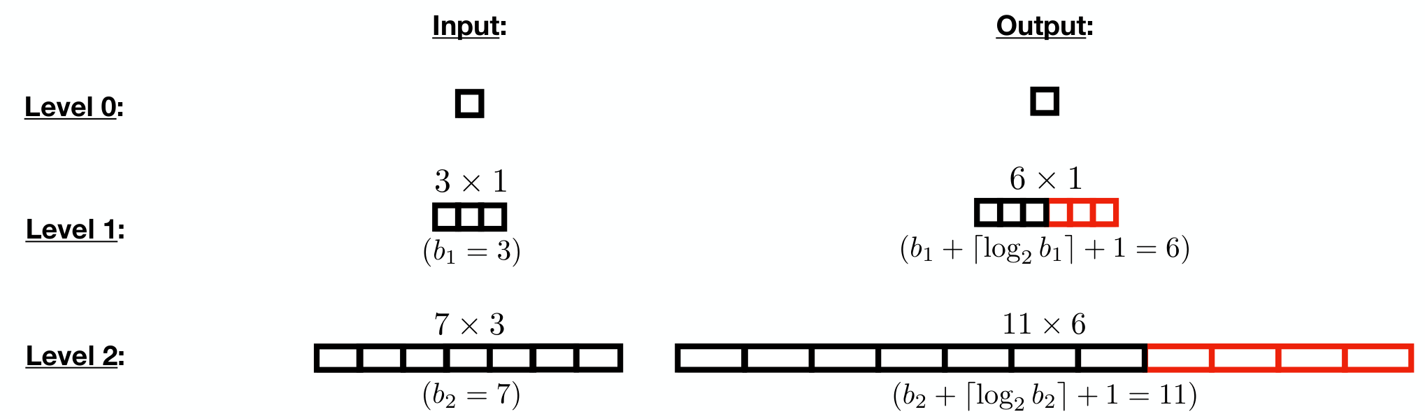
Our strategy depends on a sequence $(b_{1},b_{2},\dotsc)$; this sequence is kept fully general for now. The encoder is defined recursively according to levels indexed by $l=0,1,\dotsc,L$. The maximum level $L$ will be a function of $k$, and the levels $l=0,1,\dotsc,L-1$ will work with a smaller number of bits, denoted by $k_{l}<k$. The encoders will also add redundancy, thus outputting some number $n_{l}$ of bits with $n_{l}\geq b_{l}$. Specifically, we will have $k_{0}=n_{0}=1$, and $k_{l}=\prod_{i=1}^{l}b_{i}$ and $n_{l}=\prod_{i=1}^{l}(b_{i}+\lceil\log_{2}b_{i}\rceil+1)$ for $l\geq 1$.

The encoders are recursively defined as follows (see Figure 2 for an illustration):

• •

  A level-$0$ encoder takes in 1 bit, and simply outputs that bit. Hence, $k_{0}=n_{0}=1$.

• •

  For $l\geq 1$, a level-$l$ encoder takes in a block of $k_{l}=\prod_{i=1}^{l}b_{i}$ bits, breaks them up into $b_{l}$ blocks of length $k_{l-1}=\prod_{i=1}^{l-1}b_{i}$ each, and applies the level-$(l-1)$ encoding strategy to each block. In addition, a further $\lceil\log_{2}b_{l}\rceil+1$ redundancy blocks are generated according to Lemma 4, and they are also encoded using level-$(l-1)$ encoding. The final output is a sequence of $n_{l}=\prod_{i=1}^{l}(b_{i}+\lceil\log_{2}b_{i}\rceil+1)$ bits.

The overall encoder of $k$ bits is not precisely any of those above, but makes use of the level-$L$ encoder, where $L$ is defined to be the value such that $k_{L}\leq k<k_{L+1}$. Specifically, the message of $k$ bits is divided into $\lceil k/k_{L}\rceil\leq b_{L+1}$ blocks of $k_{L}$ bits each, padding the final block with zeros if necessary. The level-$L$ encoding strategy is then applied to each block. Note that padding the message at most doubles the message length.

We similarly recursively define a sequence of decoders:

• •

  A level-$0$ decoder simply reads the 1-bit input, and outputs it.

• •

  For $l\geq 1$, a level-$l$ decoder reads $n_{l}=\prod_{i=1}^{l}(b_{i}+\lceil\log_{2}b_{i}\rceil+1)$ bits, and breaks them into $b_{l}+\lceil\log_{2}b_{l}\rceil+1$ blocks of size $n_{l-1}=\prod_{i=1}^{l-1}(b_{i}+\lceil\log_{2}b_{i}\rceil+1)$ each. The level-($l-1$) decoding strategy is applied to each of these blocks (including the redundancy blocks). Then, the resulting (decoded) blocks are further decoded according to Lemma 4, on the assumption that at most one of the $b_{l}+\lceil\log_{2}b_{l}\rceil+1$ blocks has been corrupted.

The overall decoding strategy is to divide the $n$ received bits into $n_{L}$ blocks of size $n/n_{L}$ (divisibility holds by construction), and apply level-$L$ decoding on each one.

Our protocol depends not only on the sequence $(b_{1},b_{2},\dotsc)$ introduced above, but also on an additional sequence $(t_{1},t_{2},\dotsc)$. It is useful to think of the 1-bit protocol from Section II as having $b_{l}=3$ and $t_{l}=4$ for all $l$ (though it does not append redundancy blocks).

We first assign every node a level. Given $(t_{1},t_{2},\dotsc)$, the level of a node $j\in\{1,\dotsc,m-1\}$ is the largest integer $l$ such that $j$ is a multiple of $\prod_{i=1}^{l}t_{i}$ (we set $l=0$ if $j$ is not a multiple of $t_{1}$). As a result, between consecutive pairs of level-$l$ nodes, there are $t_{l}-1$ level-$(l-1)$ nodes. A level-$l$ node operates as follows:

• •

  Read $n_{l}=\prod_{i=1}^{l}(b_{i}+\lceil\log_{2}b_{i}\rceil+1)$ bits;

• •

  Decode these bits using the level-$l$ decoding strategy described above;

• •

  Encode the result back using the level-$l$ encoding strategy;

• •

  Transmit the resulting $n_{l}=\prod_{i=1}^{l}(b_{i}+\lceil\log_{2}b_{i}\rceil+1)$ bits to the next node.

This allocation produces some maximum level $L^{\prime}$, which may differ from the maximum level $L$ in Section IV-A. In view of this difference, if $k<k_{L^{\prime}}$, the encoder zero-pads the message to increase its length to $k_{L^{\prime}}$; our analysis in Section IV-C will be split according to whether this zero-padding is done or not. Moreover, the decoder operates at level $\max\{L,L^{\prime}\}$ regardless of divisibility by $\prod_{i=1}^{l}t_{i}$.

As with our 1-bit protocol, the propagation of information is delayed, and each node ignores any “non-specified” bits before the first “meaningful” bit is received.

We now state our main result for the multi-bit setting, which will be proved in Section IV-C.

We state this result with respect to $m\to\infty$ for convenience, but one can easily adapt the protocol and its analysis to fix $m$ and only take $k\to\infty$; intuitively, adding more hops only makes the problem more difficult. Moreover, in Corollary 2 below, we remove the condition $p<3^{-8}/4$ and give the precise scaling of the error probability.

Here we prove Theorem 4. Let $\epsilon_{l}$ denote the probability of failure associated with transmitting a length-$n_{l}$ block between two consecutive level-$l$ nodes (or from node 0 to the first one). Each associated level-$(l-1)$ block of length $n_{l-1}$ has a failure probability of at most $t_{l}\cdot\epsilon_{l-1}$, by a union bound over the $t_{l}$ level-$(l-1)$ nodes the block passes through. Hence, the probability of having two or more failures among the $b_{l}+\lceil\log_{2}b_{l}\rceil+1$ level-($l-1$) blocks is at most $\binom{b_{l}+\lceil\log_{2}b_{l}\rceil+1}{2}(t_{l}\epsilon_{l-1})^{2}$. Since the redundancy added guarantees resilience to any single corrupted block, it follows that

It is convenient to note that $b_{l}+\lceil\log_{2}b_{l}\rceil+1\leq 2b_{l}$, and accordingly simply this recursion to

We proceed with the proof of this proposition, referring to conditions (i)–(iii) throughout.

We need to show that the total transmission time associated with a message of length $k$ over $m$ hops scales as $\mathcal{O}(m+k)$. Recall the notions of transmission delay and propagation delay from Section II-B. We will show that the transmission delay scales as $\mathcal{O}(m+k)$ and the propagation delay scales as $\mathcal{O}(m)$, starting with the latter.

A level-$l$ relay node waits to receive $\prod_{i=1}^{l}(b_{i}+\lceil\log_{2}b_{i}\rceil+1)$ bits before transmitting. Hence, since there are at most $\frac{m}{\prod_{i=1}^{l}t_{i}}$ relay nodes at level $l$, the total propagation delay is at most

where $c$ is a constant such that $\prod_{i=1}^{l}(1+\frac{3\log_{2}b_{i}}{b_{i}})\leq c$ for all $l$; the existence of such a constant is guaranteed because $\sum_{l=1}^{\infty}\frac{\log b_{l}}{b_{l}}$ is finite (condition (iii)).⁶⁶ 6 This is most easily seen by applying the bound $1+z\leq e^{z}$ to the term $1+\frac{3\log_{2}b_{i}}{b_{i}}$. Since $\frac{b_{i}}{t_{i}}\leq 1/2$ (condition (ii)), we also have that $\sum_{l=1}^{\infty}\prod_{i=1}^{l}\frac{b_{i}}{t_{i}}$ is finite, and hence, the propagation delay is linear in $m$.

To analyze the transmission delay, we consider two cases.

• •

  Case 1 ($k\leq k_{L^{\prime}}$). Recall that in this case, the message is zero-padded to increase the length to $k_{L^{\prime}}$. Hence, a total of $\prod_{i=1}^{L^{\prime}}(b_{i}+\lceil\log_{2}b_{i}\rceil+1)$ bits are sent by the encoder. Observe that this is equal to the propagation delay incurred by a level-$L^{\prime}$ node, and we have already shown that this is at most $\mathcal{O}(m)$.

• •

  Case 2 ($k>k_{L^{\prime}}$). In this case, the message length is not increased, and $L$ (from Section IV-A) is the level at which the message is encoded (in $\lceil k/k_{L}\rceil\leq b_{L+1}$ blocks). The multiplicative increase in length (of the message size) due to level-$L$ encoding takes the form

  $$\prod_{l=1}^{L}\Big(1+\frac{\lceil\log_{2}b_{l}\rceil+1}{b_{l}}\Big),$$

  (20)

  which is bounded independently of $L$ since $\sum_{l=1}^{\infty}\frac{\log b_{l}}{b_{l}}$ is finite (analogous to the last step in (19)). Hence, the transmission delay is $\mathcal{O}(k)$ in this case.

References

- [1] W. Huleihel, Y. Polyanskiy, and O. Shayevitz, “Relaying one bit across a tandem of binary-symmetric channels,” IEEE International Symposium on Information Theory (ISIT), 2019.
- [2] S. Rajagopalan and L. Schulman, “A coding theorem for distributed computation,” ACM Symposium on Theory of Computing, 1994.
- [3] L. J. Schulman, “Communication on noisy channels: A coding theorem for computation,” in Proc. 33rd Annu. Symp. on Foundations of Comp. Sci. (FOCS), 1992, pp. 724–733.
- [4] ——, “Deterministic coding for interactive communication,” in ACM Symposium on Theory of Computing, 1993.
- [5] R. Gelles, A. Moitra, and A. Sahai, “Efficient and explicit coding for interactive communication,” in IEEE Annual Symposium on Foundations of Computer Science. IEEE, 2011, pp. 768–777.
- [6] E. Domanovitz, T. Philosof, and A. Khina, “The information velocity of packet-erasure links,” 2022, https://arxiv.org/abs/2201.04257.
- [7] V. Jog and P. L. Loh, “Teaching and learning in uncertainty,” IEEE Transactions on Information Theory, vol. 67, no. 1, pp. 598–615, 2021.
- [8] Y. H. Ling and J. Scarlett, “Optimal rates of teaching and learning under uncertainty,” IEEE Transactions on Information Theory, vol. 61, no. 11, pp. 7067–7080, 2021.
- [9] A. El Gamal and Y.-H. Kim, Network information theory. Cambridge University Press, 2011.
- [10] V. Y. F. Tan, “On the reliability function of the discrete memoryless relay channel,” IEEE Transactions on Information Theory, vol. 61, no. 4, pp. 1550–1573, 2015.
- [11] S. Salehkalaibar, M. Wigger, and L. Wang, “Hypothesis testing over the two-hop relay network,” IEEE Transactions on Information Theory, vol. 65, no. 7, pp. 4411–4433, 2019.
- [12] Y. Polyanskiy and Y. Wu, “Dissipation of information in channels with input constraints,” IEEE Transactions on Information Theory, vol. 62, no. 1, pp. 35–55, 2015.
- [13] S. Boucheron, G. Lugosi, and P. Massart, Concentration Inequalities: A Nonasymptotic Theory of Independence. OUP Oxford, 2013.
- [14] R. Ahlswede and P. Gacs, “Spreading of sets in product spaces and hypercontraction of the Markov operator,” The Annals of Probability, vol. 4, no. 6, pp. 925 – 939, 1976.
- [15] Y. Polyanskiy and Y. Wu, “Strong data-processing inequalities for channels and Bayesian networks,” in Convexity and Concentration. Springer, 2017, pp. 211–249.
- [16] D. J. C. MacKay, Information theory, inference and learning algorithms. Cambridge University Press, 2003.