Cooperative Multi-Agent Reinforcement Learning with Hypergraph Convolution

Various researches contribute to overcoming the multi-agent cooperation challenge. Indepent Q leanring (IQL) [8] extends the architecture of Deep Q-Learning Network (DQN) [1] to MAS. In mean field MARL, considering that each agent’s effect on the overall population can become infinitesimal [21]. Although mean filed MARL has demonstrated excellent performance in mean field games (MFGs), MFGs require homogeneous agents [22]. Recently, based on the centralized training with decentralized execution (CTDE) paradigm, some remarkable approaches such as value function decomposition [11], and multi-agent policy gradient methods [23] have been proposed. Compared with value-based methods, policy gradient methods can be easily applied to the environment with continuous actions space. In Multi-agent deep deterministic policy gradient (MADDPG) [12], the critic network takes overall individual observations and actions as inputs. As mentioned in [24], although policy gradient (PG) methods significantly outperform the QMIX in some continuous environments (multi-agent particle world environment (MPE) [12]), value-based methods achieve more sample-efficient than PG approaches in some discrete environments (SMAC).

Value decomposition methods decompose the joint state-action value function into a single global reward. On the basis of CTDE, plenty of MARL algorithms are proposed, e.g., Value-Decomposition Networks (VDN) [11], QMIX  [13], QPLEX [17]. VDN denotes the joint action value as the sum of individual action values. QMIX approximates the joint state-action value function monotonously. MMD-MIX [25] applies MMD-DQN [26] to collect randomness information in situations. Qtran [27] relaxes the constraints of joint action-value functions, but has a poor performance in some complex tasks. The most related to our work is GraphMIX [28], which combines graph neural networks (GNNs) [29] and value decomposition. However, GraphMIX only succeeds in several particular scenarios (i.e., $6h\_vs\_8z$).

GCN is proposed in [16] for classification tasks. GCN aims to capture neighborhood information for the irregular or non-euclidean nature of graph-structured data. GraphSAGE leverages the node feature information [30]. Only sampled neighbor nodes features are used for leveraging through aggregating functions. ChebNET [31] performs Fourier transform and converts spatial graph data into Fourier domain. Although GCN has been widely used in many areas, such as event detection [32] and knowledge graph [33], we select HGCN to aggregate instead of GCN. Replacing graphs with hypergraphs, Bai et al. deviate the two forms of convolution in HGCN [19]. [34] performs k-means clustering method to construct hypergraphs. The hypergraph attention mechanism has also been proposed in [19]. Hypergraphs in the hypergraph attention mechanism are also dynamic and non-binary. Reasons about our selection are elaborated in Section IV-A.

Dec-POMDP [35] describes the fully cooperative multi-agent tasks. A Dec-POMDP can be defined by a tuple $G=\langle\mathcal{S},\mathcal{U},\mathcal{P},\mathcal{Z},r,\mathcal{O},n,\gamma\rangle$. $s\in\mathcal{S}$ denotes the global state of the environment. Each agent $a\in\mathcal{A}:=\{1,\dots,n\}$ takes an individual action $u_{a}\in\mathcal{U}$ at each timestep. $\mathcal{U}$ is the action set. All the individual actions in the same timestep form a joint action $\mathbf{u}\in\bm{\mathcal{U}}\equiv\mathcal{U}^{n}$. $\mathcal{P}(s^{\prime}|s,\mathbf{u}):\mathcal{S}\times\bm{\mathcal{U}}\to\Delta(\mathcal{S})$ denotes the transition probability for any joint actions of both agents, where $\Delta(\cdot)$ is the simplex. All the agents share the same reward function $r(s,\mathbf{u}):\mathcal{S}\times\bm{\mathcal{U}}\xrightarrow{}\mathbb{R}$.

Each agent gets its own local individual partial observation $z\in\mathcal{Z}$ according to the observation function $\mathcal{O}(s,a):\mathcal{S}\times\mathcal{A}\xrightarrow{}\mathcal{Z}$. The previous of actions and observations for a agent makes up its own action-observation history $\tau_{a}\in T\equiv(\mathcal{Z}\times\mathcal{U})$. Policy of agent $a$ is represented as: $\pi_{a}(u_{a}|\tau_{a}):T\times\mathcal{U}\xrightarrow{}\left[0,1\right]$. The cumulative discounted reward in timestep $t$ is defined as $R^{t}=\sum_{l=t}^{\infty}\gamma^{l-t}r_{l}$ [36], and we aim to maximize the expected reward $\mathbb{E}_{\tau\sim\pi}[R^{0}|s_{0}]$, where $\tau$ is a trajectory and $\gamma\in[0,1)$ is the discount factor.

In Dec-PODMP, agents share the same joint reward, leading to the design of a unique reward function to train independent agents difficultly. As we have discussed in Section I, directly applying DQN for each agent without any coordination may lead to “lazy agents” [13].

Based on the CTDE paradigm, value decomposition methods learn the decomposition of the joint value function. The core of CTDE is that a centralized critic (named “mixing network” in Figure 2) guides the agents during training. This critic only exists in the training phase and has the ability to access global states, individual observations, individual action values, and actions. Besides, during the training phase, each agent can acquire neighborhood information, including individual observation, actions from other agents. During the execution phase, the centralized critic is deleted from the structure, and agents are not allowed to access neighborhood information. There are several meaningful works proposed based on value decomposition, such as VDN, and QMIX. One of the most important equation in value decomposition is Individual-Global-Max (IGM) equation [27]:

IGM assumes that the optimality of each agent is consistent with the global optimality. Almost all algorithms based on value decomposition satisfy the IGM condition and finally achieve convergence. QMIX approximates the joint state-action value function monotonously:

where $\tau_{a}$ denotes action-observation history of agent $a$, and $u_{a}$ denotes individual action of agent $a$. The joint value functions in Qtran is formulated as:

where $\phi$ varies in each method. In some complex tasks, Qtran has a poor performance. These methods (e.g., VDN, QMIX, etc.) pay more attention on decomposing the joint value function, but ignore the coordination between agents.

A hypergraph [37] $\mathcal{G}$ is consisted of a vertex set $\mathbf{V}=\{v_{1},v_{2},\dots,v_{N}\}$ ($N$ represents the number of vertices) and the edge set $\mathbf{E}$ with $M$ hyperedges. The adjacency matrix of the hypergraph $H\subseteq\mathbb{R}^{N\times M}$ indicates the connection between a vertice and hyperedge. For a vertex $v_{i}\in\mathbf{V}$ and a hyperedge $\epsilon\in\mathbf{E}$, when $v_{i}$ is connected by $\epsilon$, $H_{i\epsilon}=1$ exists, otherwise we have $H_{i\epsilon}=0$. Besides, each hyperedge $\epsilon$ has a non-negative weight $w_{\epsilon\epsilon}$. All the $w_{\epsilon\epsilon}$ is form a diagonal matrix $\mathbf{W}\in\mathbb{R}^{M\times M}$. In a hypergraph, the vertex degree $\textbf{D}\in\mathbb{R}^{N\times N}$ and the hyperedge degree $\textbf{B}\in\mathbb{R}^{M\times M}$ are defined as $D_{ii}=\sum_{\epsilon=1}^{M}w_{\epsilon\epsilon}H_{i\epsilon},\;B_{\epsilon\epsilon}=\sum_{i=1}^{N}H_{i\epsilon}$. It is noticed that D and B are diagonal matrices.

In an indirect graph, the degree of an edge is 2, presenting that each edge only connects 2 vertices. However, in a hypergraph, an edge may connect more than 2 vertices. Thus, the property of the hypergraph allows more information about the nodes included in the hyperedge. Furthermore, it is easy to incorporate prior knowledge of connections between agents by selecting various hyperedges.

Given a hypergraph $\mathcal{G}=(\bm{V},\bm{E},\bm{\Delta})$ with $N$ vertices and $M$ hyperedges, $\bm{\Delta}\in\mathbb{R}^{N\times N}$ is the hypergraph Laplacian positive semi-definite matrix [18]. Then, $\bm{\Delta}$ is factorized as $\bm{\Delta}=\bm{\Phi}\bm{\Lambda}\bm{\Phi}^{T}$, where $\bm{\Phi}=\text{diag}(\phi_{1},\dots,\phi_{n})$ is an orthonormal eigen vectors and $\bm{\Lambda}=\text{diag}(\lambda_{1},\dots,\lambda_{n})$ is an diagonal matrix whose diagonal elements are the corresponding eigenvalues. The Fourier transform [38, 16] for a signal $\bm{x}=(x_{1},\dots,x_{n})$ is defined as $\hat{\bm{x}}=\bm{\Phi}^{T}\bm{x}$. Then, the spectral convolution of signal $\bm{x}$ and filiter $\bm{g}$ is defined as:

where $g(\bm{\Lambda})=\text{diag}(\bm{g}(\lambda_{1}),\dots,\bm{(}\lambda_{n})$ is a function of the Fourier coefficients. However, the computing of our method incurs $\mathcal{O}(n^{2})$ computational complexity. To solve this problem, Feng et al. [18, 31, 16] derive spectral convolution as

where $\theta_{0}$ and $\theta_{1}$ are the parameters of filtering over all nodes. Further, with the utilization of a single parameter $\theta$ is defined as:

Then, the hypergraph convolution (HGCN) is derived as:

where P denotes the weight matrix between the $(l)-$th and $(l+1)-$th layer [19]. For each node in HGCN, more information can be accessed between those nodes connected by a common hyperedge. The greater the weights, the more information about observations, histories and actions is provided.

In Section III-C, we elaborate the definition of hypergraphs. Traditional hypergraphs usually have three drawbacks: (1) prior knowledge is required to build hypergraph, but the prior knowledge is usually hard to construct; and (2) the hypergraph is fixed when it is established, which leads to fixed connections between agents; and 3) the hypegraph only include two value (i.e., 1 or 0), indicating whether the node is connected by the hyperedge. Based on the analysis mentioned above, we rethink that agents need different levels of collaboration in different situations, e.g., in $MMM2$ agents need a high-level collaboration, but only low-level collaboration is needed for agent in $2s3z$. Surely, the traditional hypergraph can not solve these problems we mentioned.

Instead of building a fixed binary hypergraph beyond prior knowledge, we generate a dynamic hypergraph via neural networks which adjusts automatically according to the agents’ individual observations. We use real-value hypergraph to describe the connections between agents, where different values of hyperedges represent different levels of collaboration.

To describe the degrees of collaboration appropriately, we replace the original binary hypergraph with a real-value hypergraph. As mentioned in [19], non-binary hypergraphs also follow Eq. (5).

In HGCN-MIX, a linear function is utilized, which takes individual observation $z_{i}\in\mathcal{Z},i\in\{1,\dots,n\}$ as input, and generates a real values vector $\mathrm{A_{i}}\in\mathbb{R}^{m}$, where $m$ denotes the number of hyperedges. Then, under the ReLU operation, the negative weights are modified to 0. On the one hand, negative weights break the IGM equation (Eq. (1)). On the other hand, negative weights make the hypergraph irreversible. Each value in $\mathrm{A_{i}}$, denoted as $\omega_{i,j},j\in\{1,\dots,m\}$, presents the weights for hyperedge $\epsilon_{j}$. The entirety of $\omega_{i,j}$ consists of the first part $H_{1}$ of our hypergraph $H$:

The above equation lead agents to collaborate with others in different observations.

Inspired by GCN, we add an $n$-dimensional identity matrix, which is denoted as $H_{2}\subseteq\mathbb{R}^{n\times n}$, and $n$ is the number of agents. $H_{2}$ makes agents concentrate on themselves and maintain track of their own information. It is noticed that compared with $H_{1}$, a fixed value is impossibly fitness for all the environments, e.g. in $3m$, $1$ is too large but too small for $MMM2$. Therefore, we multiply $H_{2}$ by the average of $H_{1}$ to make the $H_{2}$ having the same orders as the $H_{1}$’s. Thus, we formulate $H_{2}$ as:

In some environments with weak cooperation or few account of agents, $H_{2}$ matrix paves the path for keeping their own information.

We denote the average of $H_{1}$ as $\mu$. Then, joining the two $H_{1}$ and $H_{2}$ matrices together, we reformulate the final hypergraph $H\subseteq\mathbb{R}^{n\times(m+n)}$ as:

where $\omega_{i,k},i\in[1,n],\text{and}\ k\in[1,m]$ is the weight of learned connection between agents, and $n$ denotes the number of agents and $m$ denotes the number of hyperedges, $\mu$ is the average value of $H_{1}$.

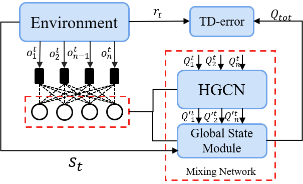
The structure of HGCN-MIX is presented in Figure 2. As shown in Figure 3(a), each agent applies a DRQN  [39] to learn individual action value $Q_{a}\in\bm{Q}$, where $a\in\{1,\dots,n\}$. Then, the hypergraph convolution performs on $\bm{Q}$. In convolution, we set P to $\mathbb{I}_{n}$, and $\mathbf{W}$ to the learned parameters. To keep Eq. (1), we use the absolute value of $\bm{W}$ for HCGN,

where $\mathbf{W}_{i},i\in\mathbb{R}$ represents the weight matrix in the $i$-th layer and $\bm{Q}^{\prime}\in\mathbb{R}^{n}$ denotes the modified action values. Each action value $Q_{a}$ appends the information contained in all the $Q_{a}$ by our method, so that agents can strengthen their collaboration. Then, a QMIX module attempts to add global state information to $\mathbf{Q}^{\prime}$ with $\mathbf{Q}^{\prime}$ as an input. As shown in Figure 3(b), $Q_{tot}$ represents the joint action value, which can be formulated as:

Our loss function follows the TD-error:

where the joint action-value function is parameterized by $\theta$, and $y_{tot}=r+\gamma\max_{\bm{u^{\prime}}}Q_{tot}(\bm{\tau^{\prime}},\bm{u^{\prime}}|\theta^{-})$. The target network is parameterized by $\theta$.

We conduct the experiments on SMAC [20] platform, which are commonly adopted to evaluate MARL algorithms. Our implementation is based on the framework for deep MARL algorithms, i.e., Pymarl [20]. Pymarl uses SMAC as the game environment and includes the implementations of QMIX, QTRAN, and VDN. The version of the Starcraft II is 4.6.2 (B69232) in our experiments¹¹ 1 Performance is NOT usually comparable between versions [20].. We select several well-known baseline algorithms include RODE [40], ROMA [41], QMIX, QTRAN [27], and VDN, as our baseline methods. Our experiments are carried out on Nvidia GeForce RTX 3090 graphics cards and Intel (R) Xeon (R) Platinum 8280 CPU. The policies are trained for 2 million timesteps.In HGCN-MIX, the number of learning hyperedge is set to 32. Other hyperparameters and the code of HGCN-MIX follow this link²² 2 https://github.com/cugbbaiyun/HGCN-MIX. We record the maximum median wining rates during the 2 million timesteps, as we shown in Table I.

In Figure 4, the solid line is the median winning rates of the 5 random seeds, and the shadow denotes the $25-75\%$ percentiles of the winning rates. The experimental results illustrate that HGCN-MIX outperforms the QMIX approach significantly. In $27m\_vs\_30m$, and $MMM2$, HGCN-MIX achieves the $20\%$ higher winning rate than baseline (i.e., QMIX). In $2s3z,5m\_vs\_6m$, and $8m\_vs\_9m$, the winning rates trend of HGCN-MIX has plateaued faster than baseline, however, in $25m,3s5z$, and $MMM$, we observe the opposite results. The learning of hypergraphs in HGCN-MIX leads to extra computational cost. In the rest 3 out 7 easy scenarios, e.g., $1c3s5z$, $3s5z$, etc., HGCN-MIX reaches a similar performance as baseline methods.

It is noticed that in the hard scenario $2c\_vs\_64zg$, the curve of winning rate in HGCN-MIX convergent unstably. There are two reasons for this phenomenon: 1) The number of ally units is 2, due to the mechanism of the game, and the two cikissis usually take the contrast actions in most scenarios. For example, a cikissi goes down and the other one always goes up. It is difficult for HGCN to learn the coordination between these two cikissis. 2) The count of enemy units is 64. A number of enemy units lead to a large action space, so that we can hardly use the 1-dimensional $Q$ value to represent individual observations and actions.

It can not be ignored that matrix multiplication and matrix inversion in HGCN-MIX bring the extra computational cost compared with QMIX. Considering the significant improvement in winning rates, we believe that this amount of extra cost is acceptable.

We perform this additional study to examine how the number of hyperedges influencing the performance of joint policies. We set the counts of hyperedges to 2, 4, 8, 16, and 32, respectively. All the hypergraphs learn without one-hot matrices. We test them on the two representative super hard scenarios: $27m\_vs\_30m$ and $MMM2$, and collect the average winning rates as we shown in Figure 5.

The result in $27m\_vs\_30m$ shows that, with the counts of hyperedges increasing, HGCN-MIX can train a stronger policy. Rather than improving the winning rates, the few hyperedges limit the cooperation between different agents. However, in $MMM2$, HGCN-MIX with few hyperedges also works well. With greater than 4 hyperedges, HGCN-MIX has reached the similar performance as baseline methods. To explore the reason that why HGCN-MIX works well in $MMM2$ with few hyperedges, we record two hypergraphs in different timesteps and the same episode in $MMM2$. We visualize the hypergraphs and present in Figure 6.

How to read Figure 6. The same lines, such as 0, 1, 2, and 8 in Figure 6(b), represent these agents that have been slain, where the health of the agent is set to 0. Individual observations in dead agents are set to the same fixed mask values (i.e., -1). Therefore, the weights generated by neural networks have the same weights. The rows include many zeros introducing the hyperedges equipped with less cooperation. Besides, we can pay attention to the weights in the same hyperedges rather than different hyperedges. The diagonal matrix $W$ (defined in Section III-C) balances the relative relationships between different hyperedges.

From Figure 6, we find that there are only 4 or 5 hyperedges learned different connections in $MMM2$. This result illustrates that only 4 or 5 essential connections exist between agents in $MMM2$. When the number of hyperedges is greater than 4, HGCN-MIX achieves a similar level of performance with the different number of hyperedges.

In ablation, we conduct two algorithms (i.e., HGCN-MIX and HGCN-MIX-OH) on $MMM2$ and $2s3z$ to emphasize the influence of the learning part in Eq. (7). Hypergraph in HGCN-MIX keeps both one-hot part and learning part, and HGCN-MIX-OH only keeps the one-hot part in Eq. (7). In HGCN-MIX-OH, weights in one-hot part are set to 1. Following Eq. (5), we can derivate that when hypergraph is set as an identity matrix, no matter what $\mathbf{W}$ is, the result of HGCN satisfies: $\bm{x}^{(l+1)}=\bm{x}^{l}$. In this way, HGCN has no effectiveness. In other words, only the global state module works in the mixing network. We conduct HGCN-MIX and HGCN-MIX-OH on the super hard scenario $MMM2$ and easy scenario $2s3z$, and record the average winning rate of the policy. It is noticed that the hyperparameters of training are the same as that of in HGCN-MIX approach.

As shown in Figure 7, in $2s3z$, both HGCN-MIX and HGCN-MIX-OH reach almost 100% winning rates, but in $MMM2$ only HGCN-MIX achieves a high winning rate. HGCN-MIX-OH only works well in some easy scenarios and fails in super hard scenarios. This demonstrates that the global state module is not the most important point for the improvement of performance. The key to enhancing the coordination lies in the learning part.

References

- [1] V. Mnih, K. Kavukcuoglu, D. Silver et al., “Human-level control through deep reinforcement learning,” nature, vol. 518, no. 7540, pp. 529–533, 2015.
- [2] D. Silver, A. Huang, C. J. Maddison et al., “Mastering the game of go with deep neural networks and tree search,” nature, vol. 529, no. 7587, pp. 484–489, 2016.
- [3] C. Gong, Y. Bai, X. Hou, and X. Ji, “Stable training of bellman error in reinforcement learning,” in International Conference on Neural Information Processing. Springer, 2020, pp. 439–448.
- [4] C. Gong, Q. He, Y. Bai, X. Hou, G. Fan, and Y. Liu, “Wide-sense stationary policy optimization with bellman residual on video games,” in 2021 IEEE International Conference on Multimedia and Expo, ICME 2021, Shenzhen, China, July 5-9, 2021. IEEE, 2021, pp. 1–6.
- [5] S. Levine, C. Finn, T. Darrell et al., “End-to-end training of deep visuomotor policies,” The Journal of Machine Learning Research, vol. 17, no. 1, pp. 1334–1373, 2016.
- [6] M. Rahmati, M. Nadeem, V. Sadhu et al., “Uw-marl: Multi-agent reinforcement learning for underwater adaptive sampling using autonomous vehicles,” in Proceedings of the International Conference on Underwater Networks & Systems, 2019, pp. 1–5.
- [7] J. Cui, Y. Liu, and A. Nallanathan, “Multi-agent reinforcement learning-based resource allocation for uav networks,” IEEE Transactions on Wireless Communications, vol. 19, no. 2, pp. 729–743, 2019.
- [8] A. Tampuu, T. Matiisen, D. Kodelja et al., “Multiagent cooperation and competition with deep reinforcement learning,” PloS one, vol. 12, no. 4, p. e0172395, 2017.
- [9] T. Zhang, Y. Li, C. Wang et al., “Fop: Factorizing optimal joint policy of maximum-entropy multi-agent reinforcement learning,” in International Conference on Machine Learning. PMLR, 2021, pp. 12 491–12 500.
- [10] G. Papoudakis, F. Christianos, A. Rahman et al., “Dealing with non-stationarity in multi-agent deep reinforcement learning,” arXiv preprint arXiv:1906.04737, 2019.
- [11] P. Sunehag, G. Lever, A. Gruslys et al., “Value-decomposition networks for cooperative multi-agent learning,” ArXiv, vol. abs/1706.05296, 2018.
- [12] R. Lowe, Y. Wu, A. Tamar et al., “Multi-agent actor-critic for mixed cooperative-competitive environments,” arXiv preprint arXiv:1706.02275, 2017.
- [13] T. Rashid, M. Samvelyan, C. Schroeder et al., “Qmix: Monotonic value function factorisation for deep multi-agent reinforcement learning,” in International Conference on Machine Learning. PMLR, 2018, pp. 4295–4304.
- [14] S. Sukhbaatar, R. Fergus et al., “Learning multiagent communication with backpropagation,” Advances in neural information processing systems, vol. 29, pp. 2244–2252, 2016.
- [15] J. Jiang, C. Dun, T. Huang et al., “Graph convolutional reinforcement learning,” arXiv preprint arXiv:1810.09202, 2018.
- [16] T. N. Kipf and M. Welling, “Semi-supervised classification with graph convolutional networks,” arXiv preprint arXiv:1609.02907, 2016.
- [17] J. Wang, Z. Ren, T. Liu et al., “Qplex: Duplex dueling multi-agent q-learning,” arXiv preprint arXiv:2008.01062, 2020.
- [18] Y. Feng, H. You, Z. Zhang et al., “Hypergraph neural networks,” in Proceedings of the AAAI Conference on Artificial Intelligence, vol. 33, no. 01, 2019, pp. 3558–3565.
- [19] S. Bai, F. Zhang, and P. H. Torr, “Hypergraph convolution and hypergraph attention,” Pattern Recognition, vol. 110, p. 107637, 2021.
- [20] M. Samvelyan, T. Rashid, C. S. De Witt et al., “The starcraft multi-agent challenge,” arXiv preprint arXiv:1902.04043, 2019.
- [21] Y. Yang, R. Luo, M. Li et al., “Mean field multi-agent reinforcement learning,” in International Conference on Machine Learning. PMLR, 2018, pp. 5571–5580.
- [22] J.-M. Lasry and P.-L. Lions, “Mean field games,” Japanese journal of mathematics, vol. 2, no. 1, pp. 229–260, 2007.
- [23] C. Yu, A. Velu, E. Vinitsky et al., “The surprising effectiveness of mappo in cooperative, multi-agent games,” arXiv preprint arXiv:2103.01955, 2021.
- [24] G. Papoudakis, F. Christianos, L. Schäfer et al., “Benchmarking multi-agent deep reinforcement learning algorithms in cooperative tasks,” in Proceedings of the Neural Information Processing Systems Track on Datasets and Benchmarks (NeurIPS), 2021. [Online]. Available: http://arxiv.org/abs/2006.07869
- [25] Z. Xu, D. Li, Y. Bai et al., “Mmd-mix: Value function factorisation with maximum mean discrepancy for cooperative multi-agent reinforcement learning,” arXiv preprint arXiv:2106.11652, 2021.
- [26] T. Tang Nguyen, S. Gupta, and S. Venkatesh, “Distributional reinforcement learning with maximum mean discrepancy,” arXiv e-prints, pp. arXiv–2007, 2020.
- [27] K. Son, D. Kim, W. J. Kang et al., “Qtran: Learning to factorize with transformation for cooperative multi-agent reinforcement learning,” in International Conference on Machine Learning. PMLR, 2019, pp. 5887–5896.
- [28] N. Naderializadeh, F. H. Hung, S. Soleyman et al., “Graph convolutional value decomposition in multi-agent reinforcement learning,” arXiv preprint arXiv:2010.04740, 2020.
- [29] F. Scarselli, M. Gori, A. C. Tsoi et al., “The graph neural network model,” IEEE transactions on neural networks, vol. 20, no. 1, pp. 61–80, 2008.
- [30] W. L. Hamilton, R. Ying et al., “Inductive representation learning on large graphs,” in Proceedings of the 31st International Conference on Neural Information Processing Systems, 2017, pp. 1025–1035.
- [31] M. Defferrard, X. Bresson, and P. Vandergheynst, “Convolutional neural networks on graphs with fast localized spectral filtering,” Advances in neural information processing systems, vol. 29, pp. 3844–3852, 2016.
- [32] T. H. Nguyen and R. Grishman, “Graph convolutional networks with argument-aware pooling for event detection,” in Thirty-second AAAI conference on artificial intelligence, 2018.
- [33] Z. Wang, Q. Lv, X. Lan et al., “Cross-lingual knowledge graph alignment via graph convolutional networks,” in Proceedings of the 2018 Conference on Empirical Methods in Natural Language Processing, 2018, pp. 349–357.
- [34] J. Jiang, Y. Wei, Y. Feng et al., “Dynamic hypergraph neural networks.” in IJCAI, 2019, pp. 2635–2641.
- [35] F. A. Oliehoek and C. Amato, A concise introduction to decentralized POMDPs. Springer, 2016.
- [36] R. S. Sutton and A. G. Barto, Reinforcement learning: An introduction. MIT press, 2018.
- [37] C. Berge, Hypergraphs: combinatorics of finite sets. Elsevier, 1984, vol. 45.
- [38] R. N. Bracewell and R. N. Bracewell, The Fourier transform and its applications. McGraw-Hill New York, 1986, vol. 31999.
- [39] M. Hausknecht and P. Stone, “Deep recurrent q-learning for partially observable mdps,” in 2015 aaai fall symposium series, 2015.
- [40] T. Wang, T. Gupta, A. Mahajan et al., “Rode: Learning roles to decompose multi-agent tasks,” arXiv preprint arXiv:2010.01523, 2020.
- [41] T. Wang, H. Dong, V. Lesser et al., “Roma: Multi-agent reinforcement learning with emergent roles,” arXiv preprint arXiv:2003.08039, 2020.