The effects of lensing by local structures on the dipole of radio source counts2021The effects of lensing by local structures on the dipole of radio source counts–References
Abstract
Our peculiar motion in a homogeneous and isotropic universe imprints a dipole in the cosmic microwave background (CMB) temperature field and similarly imprints a dipole in the distribution of extragalactic radio sources on the sky. Each of these effects have been measured, however each of these measurements give different results for the velocity of our motion through the Universe: the radio dipole measurements finds the speed of our motion to be around three times larger than that of the CMB. Here we show the effects of the previously unconstrained lensing dipole, whereby necessarily local structures (required for large angular lensing scales) will distort the distribution of radio sources on the sky. We find that the inclusion of these effects does not reduce the tension between the CMB and radio source dipole measurements however without their inclusion future extragalactic number counts could lead to incorrect inferences of our peculiar motion. In addition we can constrain the size of the lensing dipole to be at the level.
Keywords:
Large-scale structure of Universe – Weak lensing – Cosmology1 Introduction
The isotropy of the universe is an essential part of the cosmological principle; it is important that such an assumption is underpinned via careful observation. The measurement of our velocity relative to two different cosmological frames, the cosmic microwave background (CMB) and distant radio sources, find different values for the speed but are consistent for the direction of the velocity. Future extragalactic observations (SKA (Bacon et al. 2020), Rubin (Ivezić et al. 2019), Euclid (Laureijs et al. 2011)) should answer the question as to whether such a discrepancy is due to physical phenomena or a systematic observational issue.
Physical implications of a discrepancy between our relative motion to the CMB and our relative motion towards radio source counts are complex. In general it would bring into question the assumption of a homogeneous universe. However given the many successes of the CDM model it is interesting to consider other possibilities for the discrepancy. For example super-Hubble isocurvature modes could contribute significantly to the intrinsic CMB dipole (Langlois & Piran 1995). This super-Hubble mode contribution would have to be larger than the CDM intrinsic dipole, it is unclear if such a large contribution is feasible.
With the assumption that the dipole anisotropy observed in the CMB is purely kinematic, a reasonable assumption as an intrinsic dipole should have an amplitude on the order of opposed to the measured amplitude of , the CMB place by far the strongest constraints on the kinematic dipole and our motion relative to the CMB rest frame finding the speed to be [km/s] in the direction , (I 2020). This constraint is made by measuring the Doppler shift of the CMB monopole due to the observer motion.
The kinematic dipole may also be constrained through the aberration and modulation of the primordial CMB temperature fluctuations (Challinor & van Leeuwen 2002, Burles & Rappaport 2006). Also using Planck weaker constraints have placed the CMB kinematic dipole using the primordial anisotropies with (stat.) (syst.) [km/s] (Planck Collaboration XXVII 2014).
Distant radio sources are affected by our relative motion towards in a similar manner (Ellis & Baldwin 1984). The observer motion induces a dipolar pattern into the assumed isotropic distribution of radio sources on the sky via Doppler boosting which induces a frequency shift to incoming photons and a modulation of their intensity and aberration in which incoming photons are deflected towards the direction of our motion. Many constraints have been made on the kinematic dipole using this method and each of them find a consistent direction with the CMB dipole but a larger amplitude (Blake & Wall 2002,Crawford 2009, Singal 2011, Gibelyou & Huterer 2012, Rubart & Schwarz 2013,Tiwari et al. 2015,Colin et al. 2017 ). In more detail, Tiwari et al. 2015 find [km/s] using the NVSS catalog (Condon et al. 1998) and Colin et al. 2017 find the much larger [km/s] by combining the NVSS and SUMSS catalog (Mauch et al. 2003). Bengaly et al. 2019 note that linear estimators, used in many but not all radio dipole estimations, may lead to biased estimation of the amplitude and direction. Siewert et al. 2021 using a quadratic estimator performed a reanalysis of four radio catalogs (TGSS-ADR1 (Intema et al. 2017), WENSS (de Bruyn et al. 2000), SUMSS, and NVSS), and found consistent results with previous analyses, a direction in agreement with the CMB dipole but a larger amplitude.
In addition to the CMB and radio source counts there are numerous other manner to constrain the kinematic dipole such as the thermal Sunyaev-Zel’dovich (Planck Collaboration LVI 2020), the X-ray background (Plionis & Georgantopoulos 1999), galaxy cluster scaling relations (Migkas et al. 2021) and supernovae observations (Colin et al. 2019). The latter two methods also find tensions with the CMB kinematic dipole measurement.
It is also interesting to consider how local structures will magnify and shift angular positions of distant radio sources in a non-isotropic manner such that this signal could be confused with the kinematic dipole. The effects of kinematic aberration may be confused with the effects of lensing such that in many analyses (Tiwari et al. 2015, Planck Collaboration LVI 2020, Planck Collaboration XXVII 2014, Ferreira & Quartin 2020) the local lensing dipole has to be assumed to be small, by constraining the dipole in this work and constraining the dipole to be small, this is no longer an assumption.
In Section 2 we show how the motion of an observer and lensing changes the observed radio source counts on the sky. In Section 3 we discuss constraints on the lensing dipole using the density field reconstructed from low-redshift galaxy surveys. In Section 4 we present the data used in our analysis and measurements of the lensing and kinematic dipoles in radio source counts before concluding in Section 5.
2 Radio source count dipole
The lensing dipole increases the flux of incoming radiation through lensing magnification, therefore introducing faint sources into a magnitude limited sample and deflects the path of photons away from the position of the dipole, therefore reducing the number of sources such that these two effects act against one another. The lensing deflection is at some level degenerate with the aberration due to our motion.
Here we consider the combined effects of kinematic and lensing dipole. Doppler boosting will shift the observed frequency of radiation in comparison to an observer in the rest frame of the source such that the observer frequency, , can be related to the rest frame frequency, ,
| (1) |
to first order in , where for an observer moving at speed at an angle with respect to the source rest frame.
As the flux density of radio sources follows a power-law in frequency, , with (Tiwari 2019), the frequency shift will change the measured flux density at a given observed frequency.
The combined flux density change from Doppler boosting and lensing magnification is,
| (2) |
where is the observed source flux density, is the intrinsic source flux density in the absence of lensing and Doppler boosting and is the lensing convergence. The observed flux is increased by lensing due to the increase of the solid angle of the source, see for example Schmidt et al. 2009, Broadhurst et al. 1994. Additionally the solid angle on the sky is changed by aberration from the observer motion and the lensing magnification as,
| (3) |
Note that a positive lensing dipole increases the angle on the sky, whereas a positive kinematic dipole will reduce it. Combining these two effects we can consider the change in number counts at a position for a flux limited survey,
| (4) |
where is related to the slope of source flux function at the flux limit,
| (5) |
this quantity can be measured on the data. Strictly we should use the intrinsic source population instead of osberved source population after the effects of Doppler boosting and lensing, fortunately the difference between the two will be small provided varies slowly with flux.
We see that in Equation 4 there is a term proportional to the lensing convergence, , this is the term which is normally neglected in radio source count dipole analyses.
3 Local lensing dipole with Cosmic Flows
The anticipated local lensing dipole may be estimated using low-redshift galaxy surveys. We use the local luminosity-weighted galaxy density field, , provided by (Carrick et al. 2015) 11 1 https://cosmicflows.iap.fr/ which extends out to [Mpc/h] we can attempt to estimate the lensing contribution of such structures. This luminosity-weighted galaxy density field was reconstructed using the 2M++ full sky galaxy redhsift catalog (Lavaux & Hudson 2011).
In order to convert the galaxy density into a matter density we assume the bias which we obtain from Carrick et al. 2015 and taking . Taking a linear biasing relation the galaxy density is related to dark matter density as where the density contrast with the mean matter density of the universe. Subsequently we reconstruct the lensing convergence, , along the line of sight using the born-approximation and ray-tracing through the provided cosmic-flows density box with the following equation,
| (6) |
where is the comoving distance, is the Hubble constant, is the matter density and is the scale factor. These measurements are very noisy and we are unable to detect any dipolar structure in the resultant projected convergence map. This is also unsurprising in that Carrick et al. 2015 do not find evidence of a local void found elsewhere, unlike more recent cosmic-flows results (Tully et al. 2019). As these are not yet public we have used the older results.
4 Joint constraints on kinetic and lensing dipoles from radio source counts
In this section we constrain the kinematic and lensing dipole using radio source count dipole measurements. The two effects are separated by using a series of different flux density cuts.
4.1 Data
We are able to place constraints on the lensing dipole and the kinematic dipole using the results of Tiwari et al. 2015. They have measured the dipole anisotropy of radio source counts using the NRAO VLA Sky Survey (NVSS) (Condon et al. 1998). The NVSS is a radio continuum survey operating at the frequency GHz and covering the entire northern sky. The median redshift of the radio sources is at which point the effects of local structures should be negligible although they also include additional cuts which eliminates the supergalactic plane. They find consistent results for the dipole amplitude regardless of which cuts are made, indicating the contamination from local structures is negligible.
They find a much larger peculiar velocity than the CMB with [km/s]. Using the measured dipole for each flux density cut we break the degeneracy between the lensing and kinematic dipole. These measurement are summarised in Table 1, which with addition of the measurement of , is all that is needed to estimate both the lensing and kinematic dipole.
| [mJy] | ||||
|---|---|---|---|---|
| 10 | 0.902 | 0.0096 | 0.0026 | |
| 20 | 1.006 | 0.0125 | 0.0040 | |
| 30 | 1.072 | 0.0143 | 0.0048 | |
| 40 | 1.123 | 0.0136 | 0.0049 | |
| 50 | 1.168 | 0.0157 | 0.0059 |
4.2 Model
In contrast to previous work we estimate the magnitude of the lensing dipole at the same time as the kinematic dipole using the equation,
| (7) |
as the value of changes for different flux density cuts these two quantities may be constrained at the same time. We further make the simplification that the lensing dipole and kinematic dipole are aligned, such an approximation is justified as the same structures inducing the kinematic dipole should dominate the lensing dipole.
4.3 Results
Firstly we constrain the lensing and kinematic dipoles separately for each individual flux density cut with the prior that . Using a Gaussian likelihood and an MCMC analysis using the python package emcee (Foreman-Mackey et al. 2013) 22 2 https://emcee.readthedocs.io/. These constraints are shown in Figure 4. Unsurprisingly and are degenerate such that the constraint only arises due to the prior. We also see that the orientation of the degeneracy changes with the flux density limit such that the combination of these measurement can constrain both of the dipoles. It is worth noting that for the flux density cut at [mJy], the red contour in Figure 4, the source count dipole is not very sensitive to the lensing dipole, this is because at which point the effects of lensing magnification and the change in solid angle on the sky due to lensing cancel one another.

Secondly we perform a combined analysis which allows us to break the degeneracy between and , in this case we no longer require a prior on . The measurements of the dipole at each flux density cut are not independent, as the sources overlap. In order to account for this overlap we use a multivariate Gaussian likelihood and calculate the error for each component of the covariance matrix as, , where the correlation coefficent is simply the ratio of the overlap in the number of radio sources used in each measurement. In practice the errors do not significantly change when each measurement is considered to be independent. This should be considered a cautious approach given that the constraining power of each sample happens for sources at the flux density limit, naturally this is information not shared between any of flux density cuts.
We take into account errors on and by including them as nuisance parameters with Gaussian priors in our MCMC analysis. For we take its mean to be, as stated earlier with the conservative error (Tiwari 2019). For we use the values in Table 1 with errors . The inclusion of the errors on and leads to less than a 5 % increase in the errors on and . Additionally Tiwari 2019 find a slight increase of with flux density, with the large uncertainty used on in our analysis we will not be sensitive to these effects.
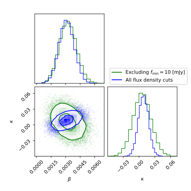
The results of the MCMC analysis, are shown in Figure 2. We obtain [km/s] and , a slightly lower speed than the results of Tiwari et al. 2015. We are able to place constraints on the lensing dipole finding that at the level. The inclusion of a lensing dipole does not help to ease the tension between the radio counts and CMB results.
We also performed an analysis excluding the 10 [mJy] flux density threshold. The motivation is that (Blake & Wall 2002) found that the NVSS survey may suffer from systematic issue below 15 [mJy]. Excluding this flux cut notably reduces the constraints on the lensing dipole, this is to be expected as seen in Figure 4 the posterior for the 10 [mJy] is orientated against the other flux density thresholds. We obtain [km/s] and .
5 Discussion and Conclusions
We have seen that we can constrain at the same time the lensing dipole and the kinematic dipole without degradation of the kinematic dipole constraints. Future surveys such as SKA (Bacon et al. 2020) in the radio and Rubin (Ivezić et al. 2019) and Euclid (Laureijs et al. 2011) in the optical will deliver large scale extragalactic catalogs with more than a billion sources at high redshifts. An improvement of four orders of magnitudes over the extragalactic catalogs used in this study. We can make a simple prediction on lensing dipole constrains with such surveys by considering the sky fraction, , covered and the number of sources, .
Considering only Poisson noise, the dominant source of noise, the variance on the measurement of the dipole is given by (Nadolny et al. 2021),
| (8) |
For SKA there should be on the order of sources and a sky fraction which gives a dipole measurement uncertainty of . Therefore assuming the lensing effects and kinematic can be completely separated, the lensing contribution is , which would imply . Therefore for SKA at the level. Similar but independent constraints will be possible with Rubin and Euclid. Detailed forecasts for the kinematic and the intrinsic clustering dipole for future surveys are provided in Nadolny et al. 2021.
To conclude, the number counts of sources on the sky will be affected by a lensing dipole induced by local structures. Such a dipole contribution is not normally considered or assumed to be small. In this work we are able to place constraints on the size of the dipole and indeed we have shown that it is small.
Acknowledgements
Calum Murray would like to thank Céline Combet for reading the manuscript and for suggestions which improved the quality of the article. Calum Murray also acknowledges support from the Labex Enigmass.
Data Availability
The data needed to reproduce the main results of this article are found in Table 1 which have been obtained by Tiwari et al. 2015 using the NVSS catalog. The data used in Section 3 can be found at https://cosmicflows.iap.fr/.
References
- Bacon et al. (2020) Bacon D. J., et al., 2020, Publications of the Astronomical Society of Australia, 37
- Bengaly et al. (2019) Bengaly C. A., Siewert T. M., Schwarz D. J., Maartens R., 2019, Monthly Notices of the Royal Astronomical Society, 486, 1350
- Blake & Wall (2002) Blake C., Wall J., 2002, arXiv preprint astro-ph/0203385
- Broadhurst et al. (1994) Broadhurst T. J., Taylor A., Peacock J., 1994, arXiv preprint astro-ph/9406052
- Burles & Rappaport (2006) Burles S., Rappaport S., 2006, The Astrophysical Journal Letters, 641, L1
- Carrick et al. (2015) Carrick J., Turnbull S. J., Lavaux G., Hudson M. J., 2015, Monthly Notices of the Royal Astronomical Society, 450, 317
- Challinor & van Leeuwen (2002) Challinor A., van Leeuwen F., 2002, Physical Review D, 65, 103001
- Colin et al. (2017) Colin J., Mohayaee R., Rameez M., Sarkar S., 2017, Monthly Notices of the Royal Astronomical Society, 471, 1045
- Colin et al. (2019) Colin J., Mohayaee R., Rameez M., Sarkar S., 2019, Astronomy & Astrophysics, 631, L13
- Condon et al. (1998) Condon J. J., Cotton W., Greisen E., Yin Q., Perley R. A., Taylor G., Broderick J., 1998, The Astronomical Journal, 115, 1693
- Crawford (2009) Crawford F., 2009, The Astrophysical Journal, 692, 887
- Ellis & Baldwin (1984) Ellis G., Baldwin J., 1984, Monthly Notices of the Royal Astronomical Society, 206, 377
- Ferreira & Quartin (2020) Ferreira P. d. S., Quartin M., 2020, arXiv preprint arXiv:2011.08385
- Foreman-Mackey (2016) Foreman-Mackey D., 2016, The Journal of Open Source Software, 1, 24
- Foreman-Mackey et al. (2013) Foreman-Mackey D., Hogg D. W., Lang D., Goodman J., 2013, PASP, 125, 306
- Gibelyou & Huterer (2012) Gibelyou C., Huterer D., 2012, Monthly Notices of the Royal Astronomical Society, 427, 1994
- I (2020) I P. C., 2020, Astronomy & Astrophysics, 641, A1
- Intema et al. (2017) Intema H., Jagannathan P., Mooley K., Frail D., 2017, Astronomy & Astrophysics, 598, A78
- Ivezić et al. (2019) Ivezić Ž., et al., 2019, The Astrophysical Journal, 873, 111
- Langlois & Piran (1995) Langlois D., Piran T., 1995, arXiv preprint astro-ph/9507094
- Laureijs et al. (2011) Laureijs R., et al., 2011, arXiv preprint arXiv:1110.3193
- Lavaux & Hudson (2011) Lavaux G., Hudson M. J., 2011, Monthly Notices of the Royal Astronomical Society, 416, 2840
- Mauch et al. (2003) Mauch T., Murphy T., Buttery H., Curran J., Hunstead R., Piestrzynski B., Robertson J., Sadler E., 2003, Monthly Notices of the Royal Astronomical Society, 342, 1117
- Migkas et al. (2021) Migkas K., Pacaud F., Schellenberger G., Erler J., Nguyen-Dang N., Reiprich T., Ramos-Ceja M., Lovisari L., 2021, Astronomy & Astrophysics, 649, A151
- Nadolny et al. (2021) Nadolny T., Durrer R., Kunz M., Padmanabhan H., 2021, arXiv preprint arXiv:2106.05284
- Planck Collaboration LVI (2020) Planck Collaboration LVI 2020, Astronomy and Astrophysics (A & A), 644
- Planck Collaboration XXVII (2014) Planck Collaboration XXVII 2014, Astronomy & Astrophysics, 571, A27
- Plionis & Georgantopoulos (1999) Plionis M., Georgantopoulos I., 1999, Monthly Notices of the Royal Astronomical Society, 306, 112
- Rubart & Schwarz (2013) Rubart M., Schwarz D. J., 2013, Astronomy & Astrophysics, 555, A117
- Schmidt et al. (2009) Schmidt F., Rozo E., Dodelson S., Hui L., Sheldon E., 2009, Physical Review Letters, 103, 051301
- Siewert et al. (2021) Siewert T. M., Schmidt-Rubart M., Schwarz D. J., 2021, Astronomy & Astrophysics, 653, A9
- Singal (2011) Singal A. K., 2011, The Astrophysical Journal letters, 742, L23
- Tiwari (2019) Tiwari P., 2019, Research in Astronomy and Astrophysics, 19, 096
- Tiwari et al. (2015) Tiwari P., Kothari R., Naskar A., Nadkarni-Ghosh S., Jain P., 2015, Astroparticle Physics, 61, 1
- Tully et al. (2019) Tully R. B., Pomarède D., Graziani R., Courtois H. M., Hoffman Y., Shaya E. J., 2019, The Astrophysical Journal, 880, 24
- de Bruyn et al. (2000) de Bruyn G., et al., 2000, VizieR Online Data Catalog, pp VIII–62