ViQUF: de novo Viral Quasispecies reconstruction using Unitig-based Flow networks
Abstract
During viral infection, intrahost mutation and recombination can lead to significant evolution, resulting in a population of viruses that harbor multiple haplotypes. The task of reconstructing these haplotypes from short-read sequencing data is called viral quasispecies assembly, and it can be categorized as a multiassembly problem. We consider the de novo version of the problem, where no reference is available.
We present ViQUF, a de novo viral quasispecies assembler that addresses haplotype assembly and quantification. ViQUF obtains a first draft of the assembly graph from a de Bruijn graph. Then, solving a min-cost flow over a flow network built for each pair of adjacent vertices based on their paired-end information creates an approximate paired assembly graph with suggested frequency values as edge labels, which is the first frequency estimation. Then, original haplotypes are obtained through a greedy path reconstruction guided by a min-cost flow solution in the approximate paired assembly graph. ViQUF outputs the contigs with their frequency estimations. Results on real and simulated data show that ViQUF is at least four times faster using at most half of the memory than previous methods,
while maintaining, and in some cases outperforming, the high quality of assembly and frequency estimation of overlap graph-based methodologies, which are known to be more accurate but slower than the de Bruijn graph-based approaches.
Availability: ViQUF is freely available at: https://github.com/borjaf696/ViQUF
1 Introduction
A host organism infected by an RNA virus, such as human immunodeficiency virus (HIV-1), typically carries a population of related but distinct viral haplotypes, i.e., viral quasispecies [1, 2], due to their high mutation rate [3]. However, it is possible to use short-read sequencing data to reconstruct the set of viral haplotypes in a sample with their relative abundance. In this work, we focus on de novo viral quasispecies assembly, which does not require a reference sequence. There are reference-based methods for viral quasispecies reconstruction [4, 5, 6]; however, this approach is constrained to well-known viruses [7] or can be biased for certain studies [8, 9].
De novo viral quasispecies assembly from shotgun reads has been tackled either using overlap graphs [8, 10] or de Bruijn graphs (DBGs) [11, 12]. Overlap graph-based approaches have traditionally been considered accurate but require many resources, whereas DBG-based approaches are usually efficient but less accurate. Recently, we showed that when properly taking advantage of paired-end reads using a paired DBG [13], a DBG-based approach can be as accurate as an overlap graph-based method [12].
Network flows have been used to solve many assembly problems in computational biology [14, 15, 16, 17, 18, 19]. These approaches first construct an assembly graph (e.g., an overlap graph, DBG, or string graph), where each vertex and edge is assigned a coverage based on the number of reads mapping to it. Then, a network flow that explains the coverage of each vertex and edge is found. Finally, the flow is split into paths, which are the contigs reported by the methods. Pevzner et al. [14] and Myers [15] first suggested using network flows to solve genome assembly. Later, Westbrooks et al. [17] used network flows in the quasispecies assembly problem. Recently, several other works have also used network flows to address the same problem [18, 20, 21, 19].
In this work, we present ViQUF, an efficient method for assembly and abundance quantification of viral quasispecies. ViQUF builds an assembly graph using the DBG paradigm and uses network flows to formulate the problem of using paired-end reads to split the assembly graph into an approximate paired assembly graph. We obtain the contigs and their frequencies from the approximate paired assembly graph by solving a network flow problem. Furthermore, we present a mathematically rigorous formulation based on kernel density estimation to determine the threshold for solid -mer abundance when building the DBG. The experimental results show that ViQUF is faster and more memory efficient than previous methods while maintaining the good quality of the resulting assembly and frequency estimation.
2 Preliminaries
Given an individual carrying a virus with reference genome and a set of haplotypes , each one with a relative frequency (or abundance), a shotgun sequencing process produces a set of reads , each read of length .
The genome is a sequence of base pairs . Each is but with three types of changes with respect to the reference genome: substitutions, insertions, and deletions.
Reads are of paired-end type; thus, each read has two parts: is the left-hand read and is the right-hand read. covers the base pairs and covers the base pairs of a haplotype . The average number of base pairs between and is called the insert size.
Due to sequencing errors, reads might include false changes of base pairs, insertions, and deletions. Given a base pair of the reference genome , there are on average reads covering it; this value is the coverage of the sequencing.
From the set of reads , our goal is to reconstruct the haplotypes in as complete as possible and estimate the relative frequency of each haplotype in the sample.
Our method is based on a DBG . The vertices are -mers, i.e., all subsequences of length of the reads in , and there is an edge between two vertices and if the last bases of match the first bases of . is a parameter of the assembly.
3 Our method: ViQUF
Figure 1 shows an overview of the steps of ViQUF. The method selects the -mers found in the reads in whose frequency is above a threshold to build a DBG. In that graph, the nonbranching paths are compacted into single nodes, unitigs, producing an assembly graph (AG). For each unitig, we associate a set of unitigs linked to it by paired-end reads. Then, AG is processed by taking every pair of adjacent nodes. For each pair, a new directed acyclic graph (DAG) is built including all unitigs linked to those two nodes by paired-end reads. We then determine a minimum path cover of DAG, where each path represents a haplotype. Therefore, the two nodes for which we computed DAG are divided as many times as paths were found.
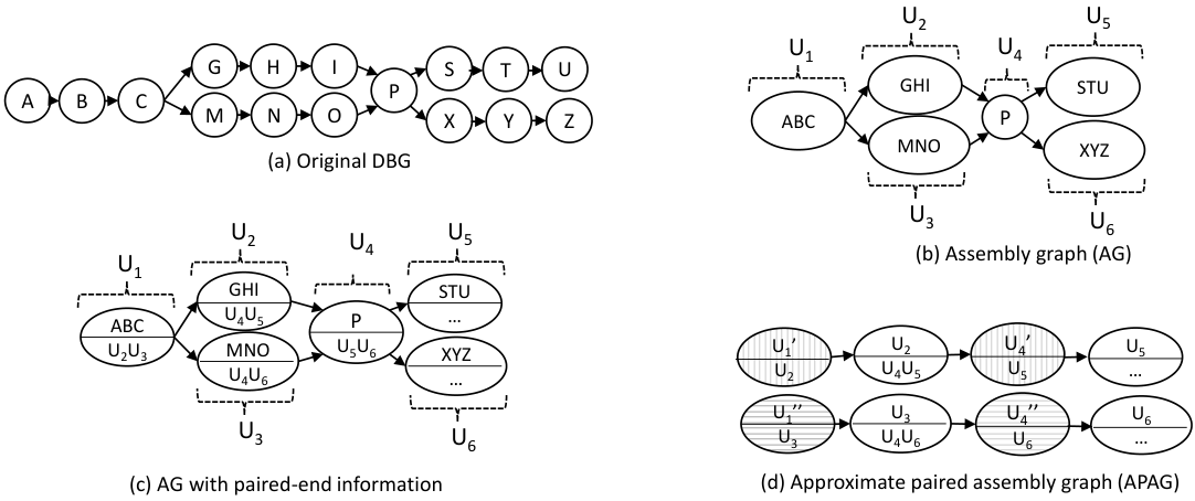
For this to work properly, each DAG must be carefully processed to achieve a more reliable graph. This includes transforming each DAG into an offset flow network and solving a min-cost flow problem. With the detected flows, the DAG is corrected, yielding a more reliable graph. Finally, the nodes of the AG are divided based on the path covers of its DAGs, and this results in a new AG, called approximate paired AG (APAG). Once this graph is polished, it is used to derive the contigs and their abundances. Figure 2 shows a running example of this process, which will be used in this section to illustrate how to build the final APAG from the original DBG.
3.1 Obtaining the AG
First we will explain in detail how AG is produced.
The nodes of AG are unitigs, i.e., compacted nonbranching paths of a DBG. Two unitigs are connected with an edge if the corresponding edge also exists in the DBG. AG is augmented with paired-end information by associating a set of paired unitigs to each unitig . The paired unitigs are inferred based on the paired-end reads.
3.1.1 Obtaining solid -mers
We denote a -mer as genomic if it appears in a haplotype of the sample and nongenomic if it does not. Recall that, in , reads contain erroneous changes of base pairs, insertions, and deletions; thus, there can be nongenomic -mers. Therefore, we use the notion of solid -mer, which denotes a -mer that occurs at least times in the reads in , where is an abundance threshold. The selection of solid -mers based on the frequency of appearance [14] works well due to the high coverage used in viral quasispecies assembly. Therefore, it is possible to establish a threshold to separate correct and erroneous information with high level of accuracy. The process is simple; the entire read set is traversed, and those -mers whose frequency is above the threshold are classified as solid, whereas the rest are considered nongenomic.
There are several methods for selecting the threshold for solid -mers. Chaisson and Pevzner [22] approximated the number of reads covering a -mer using a Poisson distribution. They selected a threshold such that few -mers are expected to be covered by several reads below that threshold. Chaisson et al. [23] applied a Poisson and Gaussian mixture model to the -mer frequency distribution, and the first local minimum is selected as the threshold. Zhao et al. [24] used a clustering method based on the variable-bandwidth mean-shift algorithm. In our recent study [12], we used a window over the -mer frequency histogram to detect the threshold value where no frequency reduction is detected.
We propose a new approach based on estimating the -mer frequency density function through kernel density estimation using the Gaussian kernel. A brief introduction of kernel density estimation can be found in the supplementary material. The frequency is expected to decrease systematically, corresponding to nongenomic -mers, up to a certain point where it stabilizes. Then, it subsequently begins to increase again, corresponding to genomic -mers. Therefore, a good threshold would be the middle point between the minimum point and the previous maximum value of the function. The problem of possible local minima can be mitigated by increasing the suggested bandwidth; thus, producing an intended over-smoothing effect in the density function, as shown in Figure 3(b).


3.1.2 Building and polishing the AG
The solid -mers obtained in the previous step are used to build a DBG. We join all the nodes of the unitigs in just one node, as shown in Figure 2(b), to reduce the number of nodes of the graph. The resulting graph is called AG. We use BCALM2 [25] to construct AG.
First, the graph is polished by removing isolated unitigs and tips shorter than a given threshold. Then, we remove filigree edges, an approach previously employed in metagenomics [26]. Filigree edges are the connections between unitigs that are not strongly supported. The idea is not to remove edges based on an overall threshold, which may remove edges corresponding to low-frequent haplotypes. Instead, edges in the graph are tagged as weak or strong based on the connection they support. For instance, the abundance of an edge , , denotes the number of reads that support the edge. Then, the abundance of a node , , is defined as the maximum over all edges incident to . Then, every edge is tagged as weak if and strong otherwise. We set the to a default value of 5, lower than the typical value used in metagenomics, where abundances are lower.
3.1.3 Adding paired-end information to the unitigs
Paired-end information is usually employed in a post-assembly step to join contigs into scaffolds such that the assembly can be extended or repetitive sections can be solved. However, this information has also been used in the previous stages of the assembly process. For instance, the approximate paired DBG (APDB) [13] is a modification of the DBG to use paired-end information directly in contig assembly. The same ideas were also employed for assembling viral quasispecies [12]. The aim is to use the paired-end information before building the contigs to untangle AG. Thus, the paired-end information is included during the graph-building step. This addition requires time and increases space consumption. However, it does not represent a problem for viral datasets in practice.
More precisely, given a -mer , its paired -mers are and a position such that .
Let be a set of -mers, denotes the unitigs where the -mers in appear. Then, given a unitig formed by -mers , its paired-end information is }. Therefore, to each vertex of the AG, we attach its .
An example of paired unitigs is shown in the supplementary material. Figure 2(c) shows our AG with paired-end information.
3.2 Building the APAG
Next, we will transform AG augmented with paired-end information to APAG. Similar to AG, the nodes of APAG are unitigs augmented with paired unitigs. However, in APAG, unitigs that occur in more than one haplotype will be replicated. Each instance of the unitig ideally corresponds to one haplotype and the paired unitigs in the same haplotype. The edges of APAG will connect the unitigs belonging to the same haplotype.
To construct APAG, we take each pair of adjacent nodes in AG and build a DAG, where its nodes are those two nodes and their paired unitigs. The DAG captures the connectivity between the unitigs in AG, by adding edges in DAG between the unitigs linked in AG through short paths. Therefore, each edge of DAG indicates that the connected nodes probably form part of the same haplotype. Then, we detect the haplotypes in that group of unitigs by finding paths in the DAG. We use that information to split the edge and the two adjacent nodes of AG according to the haplotypes found in DAG.
Therefore, DAGs are the core elements of the proposed method. This implies that they must be built with care to obtain reliable paths, including a correction based on a min-cost problem built on DAG.
3.2.1 Processing adjacent nodes: building the DAGs
Observe that if all occurrences of a unitig are due to a unique haplotype, then all paired unitigs of occur along a path in AG. Thus, they are all reachable from each other. This occurs in our example of Figure 2(c) with, e.g., , with paired unitigs and . We employ this information to detect haplotypes. For example, the pairing between and / highlights one of the two haplotypes in Figure 2: . The other haplotype is .
However, if the unitig occurs in several haplotypes, the paired -mers will span some site containing a mutation. In our example, appears in two haplotypes; thus, its paired information contains and , which are not reachable from each other. However, the paired unitigs originating from the same haplotype are reachable from each other. We will use this reachability information to split the nodes of AG into different nodes. Each node corresponds to a different haplotype; thus, producing the new APAG. The new APAG will be used to obtain the contigs.
Let be the AG. Our target is to divide the nodes in into as many nodes as the number of haplotypes they belong to. Thus, we follow the next steps:
- 1.
For each pair of adjacent nodes of , say and , a directed acyclic graph is built, where
- •
.
- •
There is an edge from to , if and only if there is a path in from to that does not include any other node in and has a length shorter than , where is the maximum error in the insert size. When searching for a path, we also limit the number of traversed branches by a threshold to ensure that the path search remains tractable. By default, we set to 10.
Observe that the nodes of DAG are the two adjacent (in AG) unitigs and , and their paired unitigs. and overlap by bp11 1 Recall that AG is a compaction of the DBG, so edges between unitigs are actually edges of the DBG, and thus the end of the source unitig overlaps bp with the beginning of the target unitig.; thus, their paired unitigs (separated from and , on average, by the insert size) should also be close by in because their distance in should not exceed , twice the insert size error if they belong to the same haplotype.
- •
- 2.
Next, we will find the source to sink paths in DAG such that the paths correspond to the haplotypes. However, not all paths correspond to haplotypes. To identify the correct paths, we will use the coverage of the DAG nodes and edges along with the paired-end information of the reads.
The coverage of the DAG edges is computed based on the coverage of the unitigs on the path in AG that the edge represents, where the coverage of a unitig is the average abundance of the -mers of the unitig. When computing the coverage of an edge of DAG, the process analyzes the paths in AG connecting them. It means that if there is only one path , the edges that reach nodes of from nodes that are not in and those coming from nodes in and reaching nodes that are not in correspond to haplotypes different from that containing and . Thus, we analyze the paths connecting and . We traverse those paths. At each node, we add to a bag the coverages of edges coming from nodes that do not belong to . Then, we distribute those excess coverages in the bag among the nodes forming a fork when we find one. Therefore, we combine the coverage and paired-end information of the reads.
The final coverage is that of the last edge of minus the incoming coverages that were not assigned to nodes leaving . The exact method for computing the coverages is described in more detail in the supplementary material.
Once the edge and node coverages are computed, we want to find a set of paths in DAG and associated abundances to explain the coverage of edges and nodes.
Figure 4 shows the process of building a reliable DAG for detecting the haplotypes that pass through the adjacent nodes and . Figure 4(a) shows AG of our running example with the coverages of nodes and edges, i.e., the number of reads supporting those nodes and edges. Figure 4(b) shows the first version of DAG . Observe that there could be two paths , and , and , , and ; thus, we must check if they are correct using the coverages of edges in AG and the paired information. Figure 4(b) shows that, even after applying the previous method for computing the coverage of the edges of DAG, the coverages may not be consistent. Observe that has two exits, adding a total output coverage of 12. This is not possible since only receives an input coverage of 10.
Figure 4: Example of the construction and coverage adjustment of DAG corresponding to the adjacent nodes and . We show the original AG, , , and
Therefore, the coverages of the graph are inconsistent. Moreover, there can be false edges due to false paths in . Their origin is due to the shared -mers between different but similar haplotypes. Additionally, there can be several real edges and thus paths, but the observed coverages may not be consistent with each other.
To solve these problems, we employ the coverage of the unitigs (nodes of DAG), i.e., the number of reads supporting them and their connections.
We need to assign a flow to the graph to satisfy the conservation property of the flow.
It means that the amount of flow reaching each node must be the same as those leaving the node. A simple heuristic, such as taking first the heaviest paths, will work accurately with a graph in that form. However, conservation is not enough; the flow assigned to each node/edge must be as close as possible to the observed coverage.
Our example, , is simple, but in a very complex graph, a decision on the flow distribution must be taken at each fork; however, the flow that reaches the fork might depend on several previous decisions. Therefore, the optimal solution is very complex. We will use a min-cost flow that will solve the two problems using a cost function, i.e., it will modify DAG such that i) satisfies the conservation law, ii) the new flow assigned to the edges is close to the observed coverage.
To assign a flow minimizing the difference from the observed coverage of the unitigs in DAG, the min-cost flow uses a cost function that increases when the difference grows. Therefore, we obtain our solution by minimizing that cost. The main advantage of this method is that it decides at all forks using a polynomial-time algorithm, minimizing the difference between the assigned flow and observed coverage globally. It means that it does not compute the best cost in the fork but computes the cost as the sum of costs at all edges of the graph to decide the flow in each edge of a fork.
With the corrected graph, the next step is to decompose the flow into paths in the graph in the most parsimonious way. Finally, the corrected flow and its decomposition into paths will give us the relative abundance of the haplotypes.
Consider the following: let be the coverage of the nodes , be the coverage of the edges , and a cost function that can be applied to nodes or edges . Following the approach proposed by [16], we use, for our problem, the same cost function for nodes and edges . Here, is the error in the frequency estimation for nodes and edges.
The objective is to find the set of paths from the sources of to the sinks of that minimizes:
where , for each path , is the estimate abundance level of the path obtained by the solution of the min-cost flow problem and the decomposition of the flow into paths.
3.2.2 Translating DAGs into offset flow networks
In this section, we explain how we use the min-cost network flows to first determine an optimal flow in DAG and then split the flow into paths. A brief introduction to network flows can be found in the supplementary material.
To determine such an optimal flow, we translate DAGs into offset flow networks and solve the min-cost problem in those offset flow networks. The min-cost flow in the offset flow network models how the coverages in DAG need to be modified to create an optimal feasible flow.
For each , we build the offset flow network as follows:
- •
Replace every node by two nodes and and two arcs: , with capacity and cost function , and with infinite capacity and the same cost function. The flow on the arc will be nonzero if the coverage of in DAG needs to be decreased in the optimal solution. However, the flow on the arc will be nonzero if the coverage of needs to be increased.
- •
Replace the arc between each pair of original nodes by two edges: with capacity , and cost function , and with infinite capacity, and the same cost function. Similarly, a nonzero flow on the forward arcs indicates that the coverage of the arc should be increased. In contrast, a nonzero flow on the backward arcs indicates that the coverage should be decreased.
- •
Add start () and target () nodes. For each source node in , add an arc from to with cost and infinite capacity. Similarly, for each target node in , add an arc from to with and infinite capacity. Source nodes are the nodes with no incoming arcs, and target nodes are the nodes with no outgoing arcs.
- •
Add an artificial source () and sink () to manage the exogenous flow and initialize the exogenous flow of each node of to . These will be used to balance the flow on nodes where the total coverage of the incoming arcs and the total coverage of the outgoing arcs do not match.
- •
For any node with
add an arc from to the node with capacity set to and cost . Update the exogenous flow of : .
- •
For any node with
add an arc from to with capacity set to and cost . Update the exogenous flow of : .
- •
Add an edge from to to close the offset network with cost and infinite capacity.
Figure 4(c) shows the resulting network flow for the offset network of of Figure 4(b). On the edges, the label means that is the node’s capacity, and is the flow that passes through it when solving the min-cost problem. Edges with only a value means that the edge has capacity, and the flow passing through it is .
3.2.3 Adjusting DAGs according to the flow in the offset flow network
Once the min-cost problem in the offset flow network is solved, the original DAG is modified as follows.
Let us consider and its . Let be the coverage of the edge , be the flow through the edge in , and be the flow through the edge in . Then, the new coverage of the edge in the modified is: .
Observe in Figure 4(d) the new , the output flows of match the input flows.
3.2.4 Obtaining paths in the new DAGs
For each adjusted , we build a set of paths from the sources to the sinks of with weights satisfying:
for all edges of .
Analogously to prior research to solve RNA-seq problems [16], we are interested in parsimoniously explaining the abundance distribution over the sample. We are interested in finding the set of paths with the lowest number of paths. A well-known result is that decomposing a flow into a minimum number of paths is an NP-hard problem in a strong sense. Therefore, only heuristic methods can be run in a reasonable time. In this work, we use a mixture of two heuristics to build the final set of paths.
We iteratively find the source to sink paths in the graph until the paths are a decomposition of the flow. We resolve branches primarily using paired-end information and secondarily choosing the heaviest path when the paired-end information is unavailable or does not point to a unique solution. To achieve this, we proceed in two steps as follows:
- •
For each node , we store the list of nodes in such that is part of their paired-end information, i.e., iff .
- •
When traversing the graph to find a path, we remember the parent of the last node on the path with an indegree greater than one. We call this saved node haplotype reference node. When we find a node with an outdegree greater than one, we must decide which branch to follow. Then, we take the haplotype reference node and employ the map built in the previous step. There are three possibilities: none of the branches of the fork is pointed by any node in the paired-end information of the haplotype reference node, then we use the heaviest path heuristic; only one branch of the fork is pointed, then we follow that path; more than one branch is pointed, then we follow the heaviest path of the pointed branches.
In the example of Figure 4(d), the only resulting path is , with weight 10. We have discarded the path , with weight 0, which, if not removed, would be responsible for mixing haplotypes.
Additionally, in DAGs, we have information about the relative abundance of the haplotypes.
3.2.5 Polishing the paths
It is necessary to solve one min-cost flow problem for each pair of adjacent nodes in AG. Ideally, the number of paths reported for each pair coincides with the number of haplotypes to which the pair belongs. However, this does not happen in practice due to, for instance, shared regions or coverage inconsistencies; thus, a wrong number of paths might be reported. Therefore, a soft polishing is performed to overcome this problem. This polishing involves tasks, such as removing paths that do not contain both nodes under study, paths with suggested flow below the -mer solid threshold, and paths with low simultaneously support from the given nodes.
The expected output once the polishing has been completed is to have for each pair of nodes both the haplotypes it belongs to and the estimation of the abundance of each haplotype given by the suggested flow.
3.2.6 Building the APAG
For each pair of adjacent nodes and in , we take the set of paths , and for each path , unless they are already in APAG, we create the nodes:
- •
, which is the node with label with paired information .
- •
, which is the node with label with paired information .
In our example, produced only one path , and . Then, we create two nodes:
As shown in Figure 2(d), APAG of our running example and our nodes and are in the upper haplotype; the remaining nodes of the haplotype are computed from DAGs and .
The nodes and correspond to the same unitig, but those nodes have different paired information, meaning that they correspond to different haplotypes.
3.3 Extracting the haplotypes and their abundances
Finally, we polish APAG by removing isolated nodes, which can be wrongly built when splitting one node more than necessary. We also remove short tips and paths with lengths below 500 bp, which are not expected to be correct contigs. After polishing APAG, the only remaining step is to traverse it and report the correct paths.
For this, we solve a min-cost flow problem on APAG. APAG is transformed into an offset network using the same method used previously for DAGs. Once the offset network is built, a min-cost flow is solved on it using cost function . Therefore, the first paths to be flooded will be the ones with more flow capacity. Then, we obtain the haplotypes and their abundances by decomposing the flow into weighted paths using a greedy algorithm to extract the heaviest path.
A similar approach has been previously introduced by VG-Flow, which solves a min-cost flow problem over a variation graph, using the number of paired-end reads mapping a particular edge as edge labels. Then, it performs a greedy path extraction to obtain the set of paths and solves a linear programming problem to polish the results. In contrast, ViQUF skips the variation graph using APAG. It also avoids mapping the reads using the suggested flows as labels for the edges. Although ViQUF could obtain the haplotype abundance estimation based on the estimated flows in APAG, the estimation for some haplotypes may not be accurate due to the lack of precision on the abundances for heads/tails plus some wrong estimations that can appear on the split computation. Therefore, like VG-Flow, ViQUF performs a flow polishing based on a simple linear programming problem. Given a graph, a set of paths on , and a flow over the paths, we define
| (1) | ||||
where and are the length and abundance of the unitig, respectively; is the -mer size, and is the flow of the path after polishing. Equation 1 minimizes the accumulated difference for each vertex and the assigned flow for each path it belongs to. The second term of the expression is a correction factor that gives a higher weight to the longest; thus, the most reliable, unitigs. The aim is to obtain, for each path, a weight that minimizes the difference between the abundance of each unitig and the given flow. Although simple, it is quite effective in practice and, even for complex cases, the frequency estimation improves significantly compared to the previous estimation.
3.4 Theoretical complexity analysis
To build the initial AG, we must build and traverse a DBG from the reads. We use GATB library [27] for this step, which takes time, where denotes the total length of all reads.
To build APAG, we need to associate each unitig with the unitigs through the paired-end information. To do so, we traverse the read set and, for each pair of -mers in the left and right reads, we locate the corresponding unitigs and add the right unitig to the set of paired unitigs of the left unitig. Assuming constant time access to the unitigs using a hash function, this takes time.
To build for two nodes and of , we traverse from the first node until we reach a specific distance (we use by default) without finding any node from . In the worst case, the number of iterations of this step is , where is the number of haplotypes. This leaves us a complexity of .
After building DAG, it is polished. For this, DAG is traversed. This costs , where and are the number of edges and vertices of , respectively. Furthermore, in the worst case , indicating that the insert size is maximum and every -mer within the insert size belongs to . In DAGs, the is bounded to . However, even in the worst case scenario, this is impossible, and the upper limit is , meaning that each node is at most connected to four other nodes. Again, the complexity of this step is also .
The third and hardest step is solving the min-cost flow problem. There are two possibilities: if the cost function is concave or convex. If it is concave, the problem is NP-hard; however, the problem can be solved in polynomial time if the cost function is convex [28]. Given a circulation problem on a network , where is a directed graph, and are non-negative functions for demand and capacity for every arc, respectively, and is a convex cost function, the minimum-cost circulation, flow, problem can be solved through cycle-canceling algorithm in , where , , is the maximum value of the costs, and is the maximum capacity in an edge. As described earlier, and ; thus, the algorithm runs in .
Finally, building and polishing DAG and solving the min-cost flow problem is repeated for each edge or pair of adjacent nodes in AG, which is four times the number of -mers in the sample in the worst case scenario. Thus, the theoretical complexity of these steps is .
The final step is to solve a minimum-cost flow over APAG, which in the worst case is the same as AG, which in the same scenario is DBG. Therefore, we can use the same previous complexity , but in this case and , resulting in a complexity of .
As summary, the entire algorithm takes . If we assume and are constants, we obtain . According to the theoretical analysis, building APAG and solving the min-cost flow in APAG are the most time-consuming steps. However, building APAG takes the longest in practice.
4 Experimental evaluation
We compare ViQUF with the most recent solutions for de novo haplotype-aware full-length viral quasispecies assembly: Virus-VG [19] and VG-Flow [29]. We also include in this comparison viaDBG [12], a related solution for de novo assembly of viral quasispecies, and PEHaplo [10] (which do not provide haplotype abundance estimations). Additionally, we compare ViQUF with two reference-based viral quasispecies construction methods: CliqueSNV [6] and PredictHaplo [5]. About parameters selections, we followed the recommendations given for all the authors in their papers. For ViQUF, we set the -mer size to 121.
4.1 Benchmarking data
In our experimental evaluation, we used simulated and real MiSeq sequencing data. We employed the methodology and datasets used by related work [8, 19, 29], which are described as follows.
Real data with ground truth. We used a gold standard benchmark for viral assembly [30]. The reads were produced from five HIV haplotypes using Illumina MiSeq (2250 bp with an error of about 0.3%) with 20000x coverage. Since the five haplotypes in the sample are known, it is possible to validate the achieved results. Table 1 presents the main characteristics of this dataset (HIV-real).
Synthetic benchmarks. Four simulated datasets were used, consisting of 2250 bp Illumina reads from different viruses: Human immunodeficiency virus (HIV), Poliovirus (POLIO), Hepatitis C virus (HCV), and Zika virus (ZIKV). These datasets correspond to those employed by [29] in their experiments. We denote these datasets by HIV-5, POLIO-6, HCV-10, and ZIKV-15, respectively. Table 1 also shows the main characteristics of these datasets.
| Virus | Genome | Average | # Haplo- | Abun- | Diver- | |
| Type | Length (bp) | Coverage | types | dance | gence | |
| HIV-real | HIV-1 | 9487–9719 | 20000 | 5 | 10%–30% | 1%–6% |
| HIV-5 | HIV-1 | 9487–9719 | 20000 | 5 | 5%–28% | 1%–6% |
| ZIKV-15 | ZIKV | 10251–10269 | 20000 | 15 | 1%–13% | 1%–12% |
| HCV-10 | HCV-1a | 9273–9311 | 20000 | 10 | 5%–19% | 6%–9% |
| POLIO-6 | Poliovirus | 7428–7460 | 20000 | 6 | 1.6%–51% | 1.2%–7% |
4.2 Evaluation metrics
For all datasets, there are ground truth sequences. Thus, we evaluate the assemblies by comparing the obtained contigs against these. We used MetaQUAST [31] for this evaluation. MetaQUAST gives multiple alignment statistics and an overall assembly evaluation. We used MetaQUAST with the option “–unique-mapping” meaning that each contig can map to only one haplotype. For each dataset, we report genome fraction retrieved, N50, and errors (misassemblies and percentage of mismatches/indels/Ns). The genome fraction is defined as the percentage of the target haplotypes contained in the set of the obtained contigs (all contigs with lengths larger than 500 bp). We used N50 to measure the fragmentation level of the assembly. The N50 is defined as the length of the shortest contigs in the assembly of at least the length of half of the total assembly. We show misassemblies to measure the behavior on repetitive sections, and error rate, which is calculated as the sum of mismatch rate, indel rate, and N-rate, measures the correctness of the assembly, showing if a set of contigs is correct or just a random graph extension. The supplementary material includes the results for the measures of precision and recall, following the extension proposed by [32] for de novo methods.
4.3 Performance analysis
| % Genome | N50 | misass- | % error | elap time | memory | MEE | |||
| dataset | method | emblies | rate | (min) | (GB) | (%) | |||
| HCV-10 | Virus-VG | 99.30% | 9231 | 0 | 0.002 | 913.48 + 1009.08 | 26.13 — 8.35 | 0.05 | 0.04 |
| VG-Flow | 99.79% | 9293 | 0 | 0.001 | 913.48 + 559.56 | 26.13 — 8.29 | 0.05 | 0.04 | |
| viaDBG | 97.72% | 8934 | 0 | 0.005 | 69.10 | 2.81 | - | - | |
| PEHaplo | 94.78% | 8661 | 0 | 0.013 | 68.45 | 8.94 | - | - | |
| PredictHaplo | 89.79% | 9273 | 0 | 0.044 | 4.11+175.73 | 0.08 — 1.14 | 6.74 | 6.44 | |
| CliqueSNV | 9.97% | 9273 | 0 | 2.100 | 4.11+3494.09 | 0.08 — 17.24 | 17.6 | 25.10 | |
| ViQUF | 97.37% | 8911 | 0 | 0.008 | 3.51 | 1.09 | 0.15 | 0.13 | |
| HIV-5 | Virus-VG | 96.85% | 9632 | 2 | 0.332 | 1619.34 + 312.68 | 26.83 — 0.64 | 6.12 | 5.57 |
| VG-Flow | 96.87% | 9625 | 2 | 0.331 | 1619.34 + 312.20 | 26.83 — 0.65 | 5.25 | 4.79 | |
| viaDBG | 97.50% | 8046 | 2 | 0.151 | 62.34 | 2.89 | - | - | |
| PEHaplo | 78.59% | 9328 | 2 | 0.690 | 73.33 | 4.84 | - | - | |
| PredictHaplo | 99.90% | 9663 | 0 | 0.591 | 4.00+120.13 | 0.09 — 1.05 | 6.26 | 5.59 | |
| CliqueSNV | 99.86% | 9649 | 0 | 1.152 | 4.00+93.67 | 0.09 — 8.51 | 7.02 | 4.06 | |
| ViQUF | 99.71% | 9237 | 2 | 0.321 | 3.26 | 1.07 | 3.09 | 1.88 | |
| POLIO-6 | Virus-VG | 89.96% | 7436 | 0 | 0.141 | 3455 + 201.23 | 17.30 — 0.73 | 1.56 | 1.18 |
| VG-Flow | 99.49% | 7388 | 2 | 0.137 | 3455 + 532.33 | 17.30 — 0.30 | 2.18 | 2.48 | |
| viaDBG | 73.81% | 1760 | 0 | 0.018 | 49.21 | 2.52 | - | - | |
| PEHaplo | 98.15% | 7428 | 0 | 0.125 | 107.96 | 3.63 | - | - | |
| PredictHaplo | 49.81% | 7428 | 0 | 0.646 | 3.80 + 82.35 | 0.10 — 0.92 | 11.08 | 11.65 | |
| CliqueSNV | 83.07% | 7428 | 0 | 1.844 | 3.8 + 27.95 | 0.10 — 8.45 | 4.74 | 5.27 | |
| ViQUF | 97.40% | 7428 | 0 | 0.247 | 2.61 | 1.06 | 3.05 | 1.79 | |
| ZIKV-15 | Virus-VG | 99.56% | 10212 | 0 | 0.077 | 706 + 407.51 | 13.45 — 1.37 | 0.94 | 0.70 |
| VG-Flow | 83.05% | 10210 | 0 | 0.144 | 706 + 406.22 | 13.45 — 0.62 | 2.00 | 1.85 | |
| viaDBG | 89.85% | 1398 | 0 | 0.110 | 65.48 | 3.25 | - | - | |
| PEHaplo | 98.32% | 10247 | 0 | 2.05 | 321.53 | 8.80 | - | - | |
| PredictHaplo | 46.65% | 10251 | 0 | 0.133 | 4.06+149.68 | 0.08 — 1.11 | 6.33 | 7.68 | |
| CliqueSNV | 66.66% | 10251 | 0 | 0.036 | 4.06 + 126.28 | 0.08 — 8.38 | 1.18 | 1.34 | |
| ViQUF | 99.08% | 10140 | 0 | 0.142 | 4.05 | 1.11 | 0.25 | 0.29 | |
| HIV-real | Virus-VG | 83.36% | 8637 | 0 | 3.384 | 3550 + 440.71 | 26.85 — 0.80 | - | - |
| VG-Flow | 89.99% | 5950 | 0 | 1.100 | 3550 + 1499.61 | 26.85 — 1.47 | - | - | |
| viaDBG | 87.25% | 1813 | 0 | 0.197 | 17.24 | 3.74 | - | - | |
| PEHaplo | 91.43% | 1262 | 0 | 0.074 | 68.34 | 3.48 | - | - | |
| PredictHaplo | 90.21% | 8702 | 0 | 0.287 | 4.71 + 100.75 | 0.09 — 0.87 | - | - | |
| CliqueSNV | 72.17% | 8676 | 0 | 1.125 | 4.71 + 136.68 | 0.09 — 9.03 | - | - | |
| ViQUF | 90.85% | 2267 | 0 | 0.292 | 3.73 | 1.07 | - | - |
In this section, we present several evaluations to verify the quality of the obtained contigs.
The de novo reconstruction methods, Virus-VG, VG-Flow, viaDBG, and PEHaplo, and the reference-based methods, PredictHaplo and CliqueSNV, were configured with the settings given by their authors [19, 29, 12, 10, 5, 6]. We use the optimal values to determine the solid -mers for viaDBG and ViQUF. A discussion on the impact of these values can be found in the supplementary material.
The results of the reference-based methods show high variability in terms of genome fraction and error rate; however, N50 is almost the length of the entire haplotype for all datasets. For example, on HCV-10, using the same alignment file, CliqueSNV only retrieves one genome, obtaining 9.97% of genome fraction, whereas PredictHaplo retrieves nine out of 10 genomes. The opposite situation occurs in POLIO-6 and ZIKV-15. On HIV-real, PredictHaplo performs well in all metrics, whereas CliqueSNV retrieves less than four of five genomes, 72.17% with a higher error rate.
The results of the de novo approaches show that although all tools have an overall good performance in terms of genome fraction, on average ViQUF achieved the highest level of genome fraction retrieved. However, there are some cases where large differences appear. The first case is POLIO-6, where viaDBG with the optimal configuration retrieves only 73% of the genome fraction, whereas the remaining methods range from 89% to 99%. In ZIKV-15, VG-Flow achieves a genome fraction of 83%, whereas the rest cover more than 89% of the genome. This difference may seem small, but the loss of one complete haplotype causes a 6% loss in genome fraction for 15 haplotypes. Finally, for HIV-5, PEHaplo achieves only 78% of the genome fraction with twice the error rate compared to the remaining de novo tools.
Analyzing the length of the obtained contigs, N50 shows that viaDBG loses by far against the rest of the tools. However, ViQUF and PEHaplo are slightly below Virus-VG and VG-Flow, but they can obtain competitive results. We note that DBG methods usually produce more fragmented assemblies than overlap methods because of using -mers instead of full-length reads.
We also evaluated the number of misassemblies and the error rate. All tools perform well in these aspects. There are only a few examples where VG-Flow, Virus-VG, and PEHaplo have quite high error rates. Virus-VG and VG-Flow have an extremely good performance on N50 but with many errors in HIV-real. Therefore, we assume that the large N50 is due to the mixing of multiple haplotypes. A similar situation occurs for PEHaplo in ZIKV-15 where the error level is very high, but N50 and genome fraction are almost perfect.
The previously published values [19, 29] did not show this anomaly. The reason is probably that Virus-VG and VG-Flow were evaluated with QUAST version 4.3, whereas we used MetaQUAST from QUAST version 5.0. Furthermore, in previous evaluations of Virus-VG and VG-Flow, contigs were allowed to align to several haplotypes, whereas we only allowed one contig to align at one place. Although one can think that this evaluation method may impact the genome fraction level, making it smaller, this is not the case since our experiment shows similar values.
Another interesting result is the misassemblies for HIV-5, where all de novo tools have at least two misassemblies. The reason for these strange results is the terminal repeats of the HIV genome. Therefore, no matter the graph methodology, if the shared region between the start and end of the genome is longer than the -mer, for DBG methods, or the average read, for overlap-based methods, they will probably extend longer than the actual genome.
The overall comparison between reference-based and de novo methods supports de novo approaches as the most reliable ones. However, the divergence levels in these datasets range from 1% to 12%, which might be high for a short-term virus infection. We have performed two extra experiments in Section 4.6 by simulating two new datasets with a divergence between 0.1% to 2%.
4.4 Haplotype abundance estimation
This section evaluates the precision of the haplotype relative frequency estimations. PEHaplo and viaDBG are excluded since they do not provide this information, as stated before. Again, we used the last version of MetaQUAST with the “–unique-mapping” set. If it is not set, one contig might be aligned to several haplotypes; thus, misplacing it and making frequency estimation harder or even impossible.
To evaluate the haplotype relative frequency estimation error, we use two different measures. More specifically, the Mean Estimation Error (MEE), which is the average error per haplotype, and the estimation error standard quasideviation (), which measures the amount of dispersion in the frequency error estimations.
We will only consider the set of contigs with N50 larger than 75% of the genome length; thus, the contigs assigned to each haplotype should be long enough to estimate the haplotype frequency. Additionally, more than one contig could cover a particular haplotype. This can happen in complex or simple datasets at the beginning and end of the haplotype, where frequencies are expected to be less reliable. For a fair comparison, the estimated frequency for one haplotype belongs to the longest contig in these situations. Besides, some short contigs sometimes appear in assemblies because of repetitive sections or failures in the assembly. These contigs are expected to have lower or inaccurate frequencies; thus, they will not be considered in the evaluation.
Table 2 presents the overall results of the five tools on the different datasets. In this experiment, from the de novo perspective, there is no clear winner. Virus-VG and VG-Flow perform better than ViQUF for HCV-10 and POLIO-6. However, ViQUF outperforms these techniques for ZIKV-15 and HIV-5, obtaining lower estimation errors and less variability. Overall, the three tools can properly estimate the haplotype frequencies for the datasets. These estimations are accurate for HCV-10 and ZIKV-15, with estimation errors per haplotype below 2% on average. However, the three techniques obtain lower levels of accuracy for POLIO-6 and HIV-5. One possible explanation is the high level of similarity between haplotypes. This high level of similarity (Table 1) means that the paired-end information of unitigs shared between two or more haplotypes point to other sets of unitigs that are also shared. Therefore, this complicates the estimation of the abundance frequencies. Nevertheless, all tools can assemble haplotypes with high levels of accuracy. However, for POLIO-6, the differences in abundance create even more problems on low abundance haplotypes with lower levels of paired-end information and a lower level of reliability on their frequencies. Finally, the reference-based methods achieve worse results, especially when they do not retrieve all haplotypes. The supplementary material contains individual estimations per haplotype and dataset for further details about which haplotypes have been retrieved and the error in each estimation.
4.5 Time performance and memory consumption
We measured the running time and peak memory usage required by the seven tools. For evaluation, we used only one core to execute the different techniques. For VG-Flow, Virus-VG, PredictHaplo and CliqueSNV, elapsed time and memory consumption are split into two terms separated by “+” and “—” symbols, respectively. For VG-Flow and Virus-VG, the first time term refers to the time required to build the preassembled contigs that the tools need, while the second term is the actual time for running the tool. The reference-based methods, PredictHaplo and CliqueSNV, require an alignment file; thus, the first term refers to the time employed to perform the alignment process. We used SAVAGE [8] to obtain the preassembled contigs as suggested by the authors of VG-Flow and Virus-VG. Additionally, we used BWA [33] to obtain the alignment files for reference-based methods. For running time, we used the symbol “+” to report the results since the entire running time is the sum of the time required by SAVAGE or BWA and the one required by a specific assembly tool. We use the symbol “—” for memory consumption, since peak memory consumption of the entire process is the maximum of both results. We decided to show the information separately because one could use another multiassembly, such as viaDBG or ViQUF, or alignment tool, such as Bowtie or Bowtie2, for this first step, which might be beneficial in terms of running times or memory consumption.
First, running times for de novo in Table 2 show that ViQUF is the fastest approach, faster than viaDBG, which is also a DBG-based method, and PEHaplo, which (although it is an overlap-based method) can correctly reduce the input data several orders of magnitude. Finally, it is significantly faster than Virus-VG and VG-Flow, based on overlap graphs. ViQUF is between 275 and 1070 times faster than SAVAGE, followed by Virus-VG, and between 275 and 1354 times than SAVAGE, followed by VG-Flow.
These results were expected since the DBG-based methods skip reads alignment, which takes quadratic time. Furthermore, ViQUF and viaDBG are faster because VG-Flow and Virus-VG require aligning reads to contigs (which takes , where is the number of contigs and is the number of reads) even without considering SAVAGE execution time, thus removing reads alignment. Compared with viaDBG and PEHaplo, ViQUF is between 5 and 80 times faster. The current implementation of ViQUF is not parallelized. The most time-consuming part of ViQUF is building APAG, which could, in principle, be computed in parallel for each pair of adjacent nodes. However, the practical impact of parallelization would be negligible since even without parallelization, ViQUF finishes in less than 5 minutes on all datasets.
For the reference-based methods, running times include the time required for alignment, even though it is negligible compared with the actual assembly time. Running times for reference-based methods are larger than those for the DBG-based methods; specifically two to four times slower than viaDBG and 10 to 40 times slower than ViQUF. These are significantly smaller than the times of Virus-VG and VG-Flow, and they are comparable with those of PEHaplo.
Finally, our entire approach is more efficient in terms of memory consumption since SAVAGE+Virus-VG and SAVAGE+Virus-Flow require 12 to 25 times the space required by ViQUF, and ViQUF requires less than half of the memory required by viaDBG and PEHaplo. However, the two reference-based methods show different behavior. While PredictHaplo is comparable to ViQUF, even outperforming its results for HIV-real, CliqueSNV requires from eight to 10 times more memory than PredictHaplo and ViQUF.
4.6 Testing de novo approaches boundaries
The experiments shown so far reveal an advantage of de novo methods against the reference-based ones. However, all datasets used in those experiments have relatively high divergence ratio between the haplotypes. Therefore, the previous sections do not include a scenario where the viruses have not evolved a lot from the common ancestor.
To test this scenario and, at the same time, test the de novo algorithms boundaries, we used FAVITES [34] and DWGSIM to simulate two different datasets with five haplotypes with low divergence ratios, from 0.1% to 2.0%. Furthermore, we have established two different abundance levels to test two different situations. In the first case we have the same abundance, 20%, for each simulated haplotype and a coverage of 20000. In the second case, we have a more realistic situation with different abundances, 33.3%, 27.6%, 20%, 12.5%,5%, and 2.5% but with a very high coverage of around 40000. Through these experiments, our goal is to test the limits of de novo and reference-based approaches in terms of sensitivity and scalability.
Table 3 summarizes the results of these experiments. In the first dataset, where abundance for each strain is the same, the reference-based methods, PredictHaplo and CliqueSNV, slightly outperform the de novo approaches. The percentage of genome retrieved is almost the same, except for CliqueSNV, which is able to obtain the five entire haplotypes with almost no error. However, mismatches here are really important, for example, PEHaplo’s 0.8 might be really problematic when maximum difference between strains is around 2%, in the case of ViQUF this number is smaller, 0.314, but it is still higher than that of the reference-based methods. In the second dataset, both reference and de novo based methods retrieve the entire set of haplotypes with a N50 as long as the actual genomes. However, in this case, there is no advantage of using reference-based methods because ViQUF retrieves the same percentage of the genome with no errors, as PredictHaplo. For the second dataset, we were not able to get results for SAVAGE+VG-Flow and CliqueSNV. SAVAGE could not produce long enough contigs in any of the experiments, whereas CliqueSNV requires more than 64Gb and thus, we could not run it on the same machine we used for the rest of the experiments. Table 3 also shows the time needed to run all the experiments. While the first dataset has the same coverage as the ones used in previous sections, the second has twice the coverage. This second dataset was simulated in this way to be able to measure the scalability of the approaches. As the results show, with the exception of CliqueSNV, the methods are scalable. PredictHaplo has the best scalability ratio, whereas ViQUF is the one with the lowest absolute runtimes.
Overall, the results exposed in Table 3 show that reference-based methods are slightly more reliable than de novo approaches when the divergence between the strains is very low, specially CliqueSNV, which has an astonishing performance. However, de novo approaches are on average faster and use less memory than the reference-based methods, even if we do not take into consideration the required time for the alignment.
| % Genome | N50 | Misassemblies | Mismatches | Time elapsed (mins) | ||
| Same abundance | ViQUF | 83.97% | 9975 | 0 | 0.314 | 4.53 |
| SAVAGE+VG-Flow | * | * | * | * | * | |
| PEHaplo | 80.00% | 10000 | 0 | 0.807 | 227.96 | |
| - 20000 coverage | PredictHaplo | 80.00% | 10000 | 0 | 0.205 | 10.53 + 442.78 |
| CliqueSNV | 100.00% | 10000 | 0 | 0.100 | 10.53 + 34.93 | |
| Different abundances | ViQUF | 99.94% | 9995 | 0 | 0.000 | 25.56 |
| SAVAGE+VG-Flow | * | * | * | * | * | |
| PEHaplo | 100.00% | 10000 | 0 | 0.604 | 1051.56 | |
| - 50000 coverage | PredictHaplo | 100.00% | 10000 | 0 | 0.100 | 23.73 + 1475.23 |
| CliqueSNV | * | * | * | * | * |
5 Conclusions
In this work, we proposed ViQUF to de novo assemble viral quasispecies. The methodology of ViQUF bears some similarity to our previous work, viaDBG [12], which also uses paired-end information to split nodes of a DBG into haplotypes. However, ViQUF includes several important improvements. First, we present a mathematically rigorous way of determining solid -mers using kernel density estimation, resulting in better estimates for the abundance threshold of solid -mers as shown by our experiments. Second, we use path cover to split the adjacent nodes into haplotypes, whereas viaDBG finds cliques in the reachability graph of paired-end nodes. Third, ViQUF uses path cover to find haplotypes and their abundances; thus, considering the coverage in this stage. However, viaDBG only reports nonbranching paths as contigs. Our experiments show that these improvements allow us to build longer contigs with comparable accuracy fast.
In the overall results, all methods show remarkable performance. In comparison, Virus-VG, VG-Flow,and the two reference-based methods (PredictHaplo and CliqueSNV) perform slightly better in average contig length than their counterparts. However, the error rate is higher than expected for some cases, and the reference-based methods lose some haplotypes. This is probably because of the high divergence between the haplotypes in each sample. However, viaDBG and ViQUF exhibit a more robust behavior without an unexpectedly high error rate for any dataset. Furthermore, ViQUF shows high levels of sensitivity, retrieving more than 90% of the genome fraction. ViQUF outperforms all methods when comparing memory consumption and runtime, especially VG-Flow and Virus-VG. It is also remarkable that PredictHaplo exhibits a great performance in running time and memory usage, especially in memory usage, where it is comparable with ViQUF and even better for real data. For this dataset, PEHaplo achieves the best performance in terms of genome fraction and error rate. ViQUF is also faster than viaDBG, using noticeably less memory. Moreover, ViQUF can provide haplotype abundance, whereas viaDBG cannot.
In summary, ViQUF obtains long accurate contigs consuming fewer resources than other methods. Furthermore, ViQUF can produce competitive haplotype frequency estimations compared with current state-of-the-art tools like Virus-VG and VG-Flow. However, our experiments were mostly conducted on synthetic data. Therefore, it is highly desirable to obtain new real datasets to conduct more thorough experimental evaluations in our future studies.
As a comparative conclusion, the viral quasispecies assembly and quantification have several good but different solutions. Some solutions are better than others depending on constraints, such as runtime, memory resources, accuracy required, and properties of a specific dataset. For example, when the sequencing depth is sufficiently high and uniform over each haplotype, and all haplotypes are completely present in the sample, ViQUF or viaDBG can be the best solution when running time and memory consumption are severe constraints. However, under the same conditions but without constraints on running time and memory, using a smart grid of parameters with SAVAGE+VG-Flow could lead to the most accurate results. Furthermore, if the average similarity between haplotypes is below 1%, the most accurate and consistent results are provided by reference-based methods.
Acknowledgments
This work has received funding from the EU H2020 under the Marie Sklodowska-Curie [GA 690941]. We wish to acknowledge the support received from the Centro de Investigación de Galicia “CITIC”, funded by Xunta de Galicia and the European Union (European Regional Development Fund- Galicia 2014-2020 Program), by grant ED431G 2019/01. This work was also supported by Xunta de Galicia/FEDER-UE under Grants [ED431C 2021/53; IG240.2020.1.185; IN852A 2018/14]; Ministerio de Ciencia e Innovación under Grants [TIN2016-78011-C4-1-R; FPU17/02742; PID2019-105221RB-C41; PID2020-114635RB-I00]; and the Academy of Finland [grants 308030 and 323233 (LS)]. The authors also thank David Posada for his advice on viral evolution.
References
- [1] E. Domingo, J. Sheldon, and C. Perales, “Viral quasispecies evolution,” Microbiology and Molecular Biology Reviews, vol. 76, no. 2, pp. 159–216, 2012.
- [2] E. C. Holmes, The Evolution and Emergence of RNA Viruses. Oxford University Press, 2009.
- [3] S. Duffy, L. A. Shackelton, and E. C. Holmes, “Rates of evolutionary change in viruses: patterns and determinants,” Nature Reviews Genetics, vol. 9, pp. 267–276, 2008.
- [4] O. Zagordi, A. Bhattacharya, N. Eriksson, and N. Beerenwinkel, “ShoRAH: estimating the genetic diversity of a mixed sample from next-generation sequencing data,” BMC Bioinformatics, vol. 12, p. 119, 2011.
- [5] S. Prabhakaran, M. Rey, O. Zagordi, N. Beerenwinkel, and V. Roth, “HIV haplotype inference using a propagating Dirichlet process mixture model,” IEEE/ACM Transactions on Computational Biology and Bioinformatics, vol. 11, no. 1, pp. 182–191, 2014.
- [6] S. Knyazev, V. Tsyvina, A. Melnyk, A. Artyomenko, T. Malygina, Y. B. Porozov, E. Campbell, W. M. Switzer, P. Skums, and A. Zelikovsky, “CliqueSNV: scalable reconstruction of intra-host viral populations from ngs reads,” bioRxiv, 2019. [Online]. Available: https://www.biorxiv.org/content/early/2019/04/22/264242
- [7] R. Malhotra, S. Prabhakara, M. Poss, and R. Acharya, “Estimating viral haplotypes in a population using k-mer counting,” in Pattern Recognition in Bioinformatics, A. Ngom, E. Formenti, J.-K. Hao, X.-M. Zhao, and T. van Laarhoven, Eds. Berlin, Heidelberg: Springer Berlin Heidelberg, 2013, pp. 265–276.
- [8] J. A. Baaijens, A. Z. E. Aabidine, E. Rivals, and A. Schönhuth, “De novo assembly of viral quasispecies using overlap graphs,” Genome Research, vol. 27, pp. 835–848, 2017.
- [9] N.-C. Chen, B. Solomon, T. Mun, S. Iyer, and B. Langmead, “Reference flow: reducing reference bias using multiple population genomes,” Genome biology, vol. 22, no. 1, pp. 1–17, 2021.
- [10] J. Chen, Y. Zhao, and Y. Sun, “De novo haplotype reconstruction in viral quasispecies using paired-end read guided path finding,” Bioinformatics, vol. 34, no. 17, pp. 2927–2935, 2018.
- [11] R. Malhotra, M. M. S. Wu, A. Rodrigo, M. Poss, and R. Acharya, “Maximum likelihood de novo reconstruction of viral populations using paired end sequencing data,” arXiv e-prints, p. arXiv:1502.04239, 2015.
- [12] B. Freire, S. Ladra, J. Paramá, and L. Salmela, “Inference of viral quasispecies with a paired de Bruijn graph,” Bioinformatics, vol. 37, no. 4, pp. 473–481, 2021. [Online]. Available: https://doi.org/10.1093/bioinformatics/btaa782
- [13] P. Medvedev, S. Pham, M. Chaisson, G. Tesler, and P. Pevzner, “Paired de Bruijn graphs: a novel approach for incorporating mate pair information into genome assemblers,” Journal of Computational Biology, vol. 18, no. 11, pp. 1625–1634, 2011.
- [14] P. A. Pevzner, H. Tang, and M. S. Waterman, “An eulerian path approach to dna fragment assembly,” Proceedings of the National Academy of Sciences, vol. 98, no. 17, pp. 9748–9753, 2001. [Online]. Available: https://www.pnas.org/content/98/17/9748
- [15] E. W. Myers, “The fragment assembly string graph,” Bioinformatics, vol. 21, no. suppl_2, pp. ii79–ii85, 09 2005. [Online]. Available: https://doi.org/10.1093/bioinformatics/bti1114
- [16] A. I. Tomescu, A. Kuosmanen, R. Rizzi, and V. Mäkinen, “A novel min-cost flow method for estimating transcript expression with RNA-Seq,” BMC Bioinformatics, vol. 14, p. S15, 2013.
- [17] K. Westbrooks, I. Astrovskaya, D. Campo, Y. Khudyakov, P. Berman, and A. Zelikovsky, “Hcv quasispecies assembly using network flows,” in Bioinformatics Research and Applications. Berlin, Heidelberg: Springer Berlin Heidelberg, 2008, pp. 159–170.
- [18] P. Skums, N. Mancuso, A. Artyomenko, B. Tork, I. Mandoiu, Y. Khudyakov, and A. Zelikovsky, “Reconstruction of viral population structure from next-generation sequencing data using multicommodity flows,” BMC Bioinformatics, vol. 14, no. 9, pp. 1–13, 2013.
- [19] J. A. Baaijens, B. Van der Roest, J. Köster, L. Stougie, and A. Schönhuth, “Full-length de novo viral quasispecies assembly through variation graph construction,” Bioinformatics, 05 2019, btz443. [Online]. Available: https://doi.org/10.1093/bioinformatics/btz443
- [20] N. Mancuso, “Algorithms for viral population analysis.” Ph.D. dissertation, Georgia State University, 2014.
- [21] I. Astrovskaya, N. Mancuso, B. Tork, S. Mangul, A. Artyomenko, P. Skums, L. Ganova-Raeva, I. Mandoiu, A. Zelikovsky, and M. Park, “Inferring viral quasispecies spectra from shortgun and aplicon next-generation sequencing reads,” in Genome analysis: current procedures and applications, M. S. Poptsova, Ed. Caister Academic Pres, 2014.
- [22] M. J. Chaisson and P. A. Pevzner, “Short read fragment assembly of bacterial genomes,” Genome Research, vol. 18, no. 2, pp. 324–330, 2008.
- [23] M. J. Chaisson, D. Brinza, and P. A. Pevzner, “De novo fragment assembly with short mate-paired reads: Does the read length matter?” Genome Research, vol. 19, no. 2, pp. 336–346, 2009.
- [24] X. Zhao, L. E. Palmer, R. Bolanos, C. Mircean, D. Fasulo, and G. M. Wittenberg, “Edar: an efficient error detection and removal algorithm for next generation sequencing data,” Journal of computational biology, vol. 17, no. 11, pp. 1549–1560, 2010.
- [25] R. Chikhi, A. Limasset, and P. Medvedev, “Compacting de Bruijn graphs from sequencing data quickly and in low memory,” Bioinformatics, vol. 32, no. 12, pp. i201–i208, 06 2016.
- [26] S. Nurk, D. Meleshko, A. Korobeynikov, and P. Pevzner, “metaSPAdes: a new versatile metagenomic assembler,” Genome Research, vol. 27, pp. 824–834, 2017.
- [27] E. Drezen, G. Rizk, R. Chikhi, C. Deltel, C. Lemaitre, P. Peterlongo, and D. Lavenier, “GATB: genome assembly & analysis tool box,” Bioinformatics, vol. 30, no. 20, pp. 2959–2961, 2014.
- [28] A. Tomescu, V. Mäkinen, F. Cunial, and D. Belazzougui, “Genome‑scale algorithm design,” 2015.
- [29] J. A. Baaijens, L. Stougie, and A. Schönhuth, “Strain-aware assembly of genomes from mixed samples using flow variation graphs,” bioRxiv, 2020. [Online]. Available: https://www.biorxiv.org/content/early/2020/02/11/645721
- [30] F. D. Giallonardo, A. Töpfer, M. Rey, S. Prabhakaran, Y. Duport, C. Leemann, S. Schmutz, N. K. Campbell, B. Joos, M. R. Lecca, A. Patrignani, M. Däumler, C. Beisel, P. Rusert, A. Trkola, H. F. Günthard, V. Roth, N. Beerenwinkel, and K. J. Metzner, “Full-length haplotype reconstruction to infer the structure of heterogeneous virus populations,” Nucleic Acids Research, vol. 42, no. 14, p. e115, 2014.
- [31] A. Mikheenko, V. Saveliev, and A. Gurevich, “MetaQUAST: evaluation of metagenome assemblies,” Bioinformatics, vol. 32, no. 7, pp. 1088–1090, 2016.
- [32] A. Eliseev, K. M. Gibson, P. Avdeyev, D. Novik, M. L. Bendall, M. Pérez-Losada, N. Alexeev, and K. A. Crandall, “Evaluation of haplotype callers for next-generation sequencing of viruses,” Infection, genetics and evolution: journal of molecular epidemiology and evolutionary genetics in infectious diseases, vol. 82, p. 104277, August 2020. [Online]. Available: https://europepmc.org/articles/PMC7293574
- [33] H. Li and R. Durbin, “Fast and accurate long-read alignment with Burrows-Wheeler transform.” Bioinformatics, vol. 26, no. 5, pp. 589–595, 2010.
- [34] N. Moshiri, M. Ragonnet-Cronin, J. O. Wertheim, and S. Mirarab, “FAVITES: simultaneous simulation of transmission networks, phylogenetic trees and sequences,” Bioinformatics, vol. 35, no. 11, pp. 1852–1861, 11 2018. [Online]. Available: https://doi.org/10.1093/bioinformatics/bty921