On the Physical Layer Security Performance over RIS-aided Dual-hop RF-UOWC Mixed Network
Abstract
Abstract
Since security has been one of the crucial issues for high-yield communications such as G and G, the researchers continuously come up with newer techniques to enhance the security and performance of these progressive wireless communications. Reconfigurable intelligent surface (RIS) is one of those techniques that artificially rearrange and optimize the propagation environment of electromagnetic waves to improve both spectrum and energy efficiency of wireless networks. Besides, in underwater communication, underwater optical wireless communication (UOWC) is a better alternative/replacement for conventional acoustic and radio frequency (RF) technologies. Hence, mixed RIS-aided RF-UOWC can be treated as a promising technology for future wireless networks. This work focuses on the secrecy performance of mixed dual-hop RIS-aided RF-UOWC networks under the intercepting effort of a probable eavesdropper. The RF link operates under generalized Gamma fading distribution; likewise, the UOWC link experiences the mixture exponential generalized Gamma distribution. The secrecy analysis subsumes the derivations of closed-form expressions for average secrecy capacity, exact and lower bound of secrecy outage probability, and strictly positive secrecy capacity, all in terms of Meijer’s functions. Capitalizing on these derivations, the effects of heterodyne and intensity modulation/direct detection systems, underwater turbulence resulting from air bubble levels, temperature gradients, and salinity gradients, are measured. Unlike conventional models that merely deal with thermally uniform scenarios, this proposed model is likely to be unique in terms of dealing with secrecy analysis of a temperature gradient RIS-aided RF-UOWC network. Lastly, the derivations are validated via Monte-Carlo simulations.
Keywords
Mixture exponential generalized Gamma, physical layer security, reconfigurable intelligent surface, underwater optical wireless communications.
1 Introduction
1.1 Background and Literature Study
The fifth generation (G) wireless communications, performing with inflated data rates, highly capable base stations, and low latency, plays a pivotal role to provide robust development of billions of devices [1]. This technological blessing helps to fulfil the essential need, complying with larger data traffic of mobile communications in every sphere. To adapt with the current situation, researchers offered and installed different solutions such as mmWaves, massive multiple-input and multiple-output (m-MIMO), small cells technique, reconfigurable intelligence surface (RIS), non-orthogonal multiple access (NOMA), ultra-dense heterogeneous networks, etc., incorporating both free space and underwater optical wireless communication (UOWC) networks that ensure expected performance according to the global traffic demand [1, 2].
Reconfigurable intelligent surfaces (RIS) are drawing enormous attention of the research community as an efficient mechanism for future secure wireless communication systems. This technology has significantly enhanced the communication quality by making the propagation environment programmable [3]. A good number of outstanding features of RIS such as passive beamforming, and customization of propagation medium by means of adjustable phase and amplitude, have created a new era in wireless communications [4]. In fact, the RIS is made of low cost and energy efficient reflecting reconfigurable elements that can reflect the incoming signals inducing modifiable phase shifts, which are further adjusted and then aligned towards the desired destination. Some promising applications are installed using RIS techniques, e.g., enhancing the m-MIMO systems, maximizing signal-to-noise ratio (SNR), promoting the signal coverage, optimising the beamforming of multi-user channels [3], etc.
In [5], a realistic RIS-based system was presented where the authors obtained higher energy efficiency in comparison with the simple amplify-and-forward (AF) multi-antenna systems. An RIS-assisted multiple-input single-output (MISO) network was studied in [6] where the author found that RIS with small number of passive elements outperforms half-duplex relaying but RIS with large number of passive elements is needed to outperform the full-duplex relaying. In [7], RIS-aided NOMA network was developed that showed superior performance relative to other orthogonal networks regarding spectral efficiency (SE), energy efficiency (EE), outage probability, and ergodic capacity. RIS-assisted optical wireless communication networks were also gaining popularity where the RIS is utilized along with the optical networks in order to promote the system performance with an improved coverage [8, 3]. RIS was used as a promising solution for free-space optical (FSO) communications to overcome atmospheric turbulence problem and pointing error issues in [9, 10, 11]. The performance of RIS-empowered FSO system was demonstrated unifying Fisher–Snedecor (), Gamma-Gamma (GG), and Málaga () distributions in [12]. RIS-assisted decode-and-forward (DF) relaying UOWC system was investigated in [13] where the authors showed the RIS element numbers, detection techniques, and UOWC optical turbulence, all affect overall system outage probability and average bit error rate (ABER). The effect of interference in a FSO-radio frequency (RF) system assisted by RIS is observed in [14] where the authors showed that the performance of this scenario can be improved by increasing FSO apertures.
UOWC is playing a leading key role in real-time sub-sea disciplines such as oceanography, offshore communications, sea climate observations, military, industry, and various sea-related engineering research activities [15]. In modern times, four types of major communications are included in UOWC: Acoustic wave (AW) communications, FSO communications, RF communications, and magnetic induction (MI) communications [16]. The transmitting signal of UOWC is generated from conical beams of laser or LED lights and - nm spectrum band at blue or green portion of seawater [17]. This technology might be a promising solution of high data-rate, bandwidth, transmission security, seawater attenuation, and it also hugely impacts low cost LEDs, digital signal processing, digital multiplexing, and digital communications [15]. The widely used UOWC model is the mixture exponential generalized Gamma (mEGG) model since this model provides a good fit for all the experimental data and at the same time it possesses good analytical properties. The expressions of ABER and outage probability of RF-UOWC system were analyzed both in closed-forms and asymptotically in [18]. The RF link was further generalized in [19]. In [20], a dual-hop FSO-UOWC system was shown where authors noticed significant impacts of the pointing errors, water bubbles, and temperature gradients on the system performance.
Since the people are relying heavily on the wireless networks for exchanging private information, the capability of sharing secret information in the presence of eavesdroppers is extremely important. In this respect, physical layer security (PLS) approach proposed by [21] is growing popularity that eliminates the pitfalls of secret key management in the classical cryptographic methods [22]. RIS can be a promising solution for PLS because of two reasons: (a) RIS makes the main channels stronger relative to the eavesdropper channels as a result of co-phasing all the reflected signals with the received transmitted signal via the direct link, and (b) RIS suppresses the eavesdroppers’ channel if the eavesdropper receives the reflected signal with opposite phase with respect to that of the transmitter. In [23], a beamforming and jamming technique were presented jointly to analyze the secrecy performance without any eavesdropper’s channel state information (CSI). The impacts of colluding and non-colluding eavesdroppers assuming a discrete phase shift at the RIS was shown in [24] in terms of ergodic secrecy rate. The PLS in vehicular network was described in [4], where the transmission is dependent on RIS, source power, eavesdroppers’ position, and distance. Relative to the RF links that can easily be wiretapped, the optical link exhibits more secure characteristics [25, 26, 27]. A DF related RF-UOWC network was shown in [27], where the secrecy outage performance was exhibited using EGG model for the UOWC link, which is further generalized using mEGG model in [19]. The same UOWC model was also utilized by [2], where the authors demonstrated that transmit antenna selection / maximal ratio combining (TAS / MRC) diversity can reduce the detrimental impacts of underwater turbulence (UWT). An innovative approach was used in the case of a highly secure underwater communication scenario considering cross layering and context-centric networking with state-of-the-art counter measurement in [28]. In [29], the average secrecy capacity (ASC) and secrecy intercept probability (SIP) performances of RF-UOWC system were shown. SIP was also analyzed in [30] with amplify-and-forward (AF) relaying making use of the MRC technique at the relay.
1.2 Motivation and Contributions
Over the recent times, researchers have proposed a few number of security models over UOWC channels and most of the proposed models are related to the relay assisted RF-UOWC mixed systems. Specifically, there exists no analysis in the literature on the security domain of RIS-assisted UOWC model. Hence, secrecy performance analysis over RIS-aided RF-UOWC system, to the very best of authors’ knowledge based on the open literature, can be seen as a novel application scenario. In this regard, we propose a RIS-aided RF-UOWC mixed network wherein the RF link follows GG distribution and the UOWC link undergoes mEGG distribution. A relay node, which exists in between the system source and the user as the destination, performs three tasks accordingly: Receiving RF signals from the source, transforming the signal to an optical structure, and passing the signal to the targeted user through the UOWC link. when the relay accepts the RF signal, an eavesdropper simultaneously receives the transmitted data from the same RF link. As compared to the Rician fading channel in [31], the offered Nakagami- model offers a more versatile scenario and several classical RIS models (e.g. Rayleigh in [32]) can be shown as a special case of this model for various values of its shape parameter. On the other hand, the considered mEGG model has the capability to adopt all of the pragmatically occurred physical transformations such as UWT, air bubbles, temperature gradient, and water salinity [17], [29]. Besides, this model also serves as one of the best models facilitating a lot of analytical tractability in deriving expressions of secrecy performance metrics. For instance, the widely used EGG model can be obtained as a special case of mEGG model [33]. The major contributions of this research are mentioned as follows:
- 1.
At first, we drive the cumulative density function (CDF) of the dual-hop SNR for the RIS-aided RF-UOWC network. Note that the proposed RIS-aided network over (Nakagami-)-mEGG model represents a unique application scenario, and hence the derived CDF is also unique. As compared to [3], we consider both RIS-aided RF links i.e. both source-to-RIS and RIS-to-relay follow Nakagami- distribution whereas [3] assumed RIS-to-relay link only to follow the Rayleigh model that is a mere special case of the proposed model.
- 2.
The secrecy performance of the proposed network is demonstrated with respect to the average secrecy capacity (ASC), exact and lower bound of secrecy outage probability (SOP), and strictly positive secrecy capacity (SPSC), etc., expressions in closed-form and further corroborated via Monte-Carlo (MC) simulations. To the best of authors’ knowledge based on the open literature, these expressions are novel and generalized, and can be utilized to unify versatile classical existing models.
- 3.
Capitalizing on the derived expressions, noticeable impacts of air bubbles and temperature gradients based UWTs for both salty and fresh waters along with the RIS-aided RF channel parameters are also demonstrated. At last, we analyse effects of two types of detection techniques i.e. intensity modulation/direct detection (IM/DD), and heterodyne detection (HD) techniques wherein the HD technique seems more efficient in secrecy improvement relative to the IM/DD technique.
1.3 Organization
The paper’s subsequent parts are categorized as follows. The proposed system, a mixed RIS-aided RF-UOWC model, and the PDFs and CDFs for each individual links are represented in Section II. Section III mathematically demonstrates the derivation of the expressions for ASC, exact SOP, lower bound of SOP, and SPSC. Numerical and simulation results are explained in Section IV. Finally, Section V summarizes the output of our works.
2 System Model and Problem Formulation
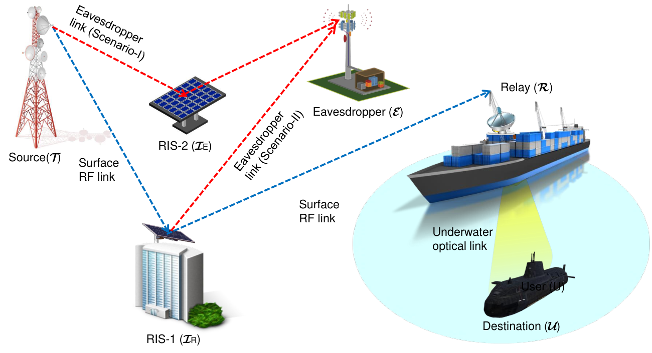
As demonstrated in Fig. 1, we present the system model of a generic dual hop RIS-aided RF-UOWC system consisting of a source , an intermediate relay (), two RISs, and , and a destination user that is stationed underneath the water surface. The distance between and is assumed very large, and due to the environmental structures between these two nodes, and are not connected via any direct link. Hence, the transmitted signal from is first sent to that in turn reflects it to . The RIS is assumed to be capable of obtaining the CSI of the link and this CSI is further utilized to maximize the received SNR at . Mainly, we can adjust the RIS induced phases to maximise the received SNR at by means of necessary phase cancellations and appropriate alignment of reflected signals from RIS [34]. The private RIS-aided communication between and through is overheard by a fortuitous eavesdropper that attempts to wiretap using similar RIS aided link. We consider following two eavesdropping scenarios.
- •
In Scenario-I, and utilize two different RISs, i.e., and , respectively. Hence, the received incoming reflected signals at and are also different.
- •
The Scenario-II assumes there exists only one RIS and both and receive the same reflected signal from . It is noteworthy that Scenario-II can be achieved as special case of Scenario-I.
Similar to [35], the RIS is assumed unaware of the eavesdropper’s CSI and hence, the considered model represents a passive eavesdropping scenario. Recently, this particular framework is more appreciable because of performing better than conventional schemes and also satisfying all the requirements demanded by several emerging applications such as unmanned aerial vehicles (UAVs) [36], large intelligent surfaces/antennas (LISA) technology [37], undersea vehicles [15], industrial IoT [38], etc. Herein, and are provided with a single antenna while is furnished with a single transmit aperture along with a single receive antenna. To receive the optical wave, has a single photo detector while and have and number of reflecting elements, respectively. As is not directly connected to , we consider overall transmission to occur in two hops. In the first hop, the system model considers to transmit signals aided with a RIS via the link to reach in the presence of that uses the same () / another () RIS-aided RF link () to conduct surveillance. The surface RF networks using , , and links follow the Nakagami- fading distribution. The relay is utilized to transform the received RF signal into respective optical form and then redirects it to the underwater user . This underwater network utilizing UOWC link experiences mEGG distribution.
2.1 SNRs of Individual Links
For Scenario-I, let us denote () and () as the first hop channel gains of the and links, respectively. Similarly, the second hop channel gains of the and links are denoted by and , respectively. Hence, the received signals at and are, respectively, given by
| (1) | ||||
| (2) |
For these concerned channels, we have , , , and , where , , , and are the Nakagami- distributed random variables (RVs), , , , and are the phases of the channel gains, , denote the adjustable phases produced by the -th and -th reflecting element of the RISs, symbolises the transmitted data symbol from with power , and , are the additive white Gaussian noise (AWGN) samples with , representing the noise power of the corresponding channels. In matrix form, (1) and (2) are written as
| (3) | ||||
| (4) |
where , , and denote the channel coefficient vectors, and and are the diagonal matrices that incorporates the phase shifts applied by the RIS elements. We can now represent the instantaneous SNRs at and as
| (5) | ||||
| (6) |
It is noteworthy the optimal choice of and that maximizes the instantaneous SNR is and , respectively. Hence, the maximized SNRs at and are expressed as
| (7) | ||||
| (8) |
where denotes the average SNR of the link and indicates the average SNR of link.
Special Case:
The received signals corresponding to Scenario-II are expressed similar to (1) and (2) while considering and with adjustable phase induced by . The corresponding maximised SNRs are obtained by letting RVs as
| (9) | ||||
| (10) |
where and are Nakagami- distributed RVs. Note that the SNRs and are referred to as and in the remaining manuscript, respectively.
Denoting the direct channel gain between and as , the expression for received signals at is expressed as
| (11) |
where exemplifies optical noises imposed at and is noise power at the destination. The corresponding SNR is given as
| (12) |
Note that the gain related to electrical-to-optical conversion while relaying is incorporated altogether in the link gain. The received SNR of the combined RIS-aided RF-UOWC system while utilizing AF variable gain relaying scheme is given as [39, Eq. (28)]
| (13) |
2.2 PDF and CDF of
The PDF of (Scenario-I) is expressed as [40, Eq. (2)]
| (14) |
where , , , , and . For the first hop of link, and denote the fading parameter and scale parameter or mean power (second moment), respectively, and for the second hop they are denoted by and , respectively, where designates the Gamma operator. The CDF of is defined as
| (15) |
Substituting (14) in (15) and exploiting [41, Eq. (3.381.8)], is followed as
| (16) |
where is the lower incomplete Gamma function [41, Eq. (8.350.1)]. Exploiting identity [41, Eq. (8.354.1)], (16) becomes
| (17) |
where and .
2.3 PDF and CDF of
The UOWC link follows mEGG distribution. The PDF of considering both HD and IM/DD techniques is as [17]
where , , , , , , , , signifies the mixture weight, designates the exponential distribution parameter, and denotes the electrical SNR of UOWC link. Here, , , and indicate the GG distribution parameters and is the Meijer’s function [41]. Detection technique is indicated by that formulates HD technique for and IM/DD technique for conditions. Electrical SNR for HD technique and IM/DD technique are specified as and , respectively.
To speculate the effects of several bubble levels and temperature gradients on turbulence scenarios and water salinity, values of , , , , and went under trial run in [17]. Table of [19] shows the increase in air bubble levels denoted by with temperature gradient denoted by that produces weak, average, and strong turbulence conditions, respectively. On the other hand, water salinity considering thermally uniform UOWC network is observed in Table of [19] to present different turbulence scenarios due to several air bubble levels for both fresh and salty waters. Hence, mEGG model helps to carry performance analysis under different turbulence scenarios in both thermal gradient and thermally uniform UOWC systems that makes this model more acceptable in the research field. Following the similar process as in (15), the CDF for the SNR of UOWC link is expressed as [17]
where and .
2.4 PDF and CDF of
Presuming link (Scenario-I) also considers Nakagami- distribution, the PDF and CDF of are expressed as [42, Eq. (2) and (3)]
| (22) |
and
| (23) |
where =, =, , , , and . For the first hop of link, and denote the fading parameter and scale parameter (second moment or mean power), respectively, whereas for the second hop, they are denoted by and , respectively. Note that for , , and , Scenario-I reduces to Scenario-II.
2.5 CDF of SNR for Dual-hop RIS-UOWC Link
The CDF of is expressed as [43, Eq. (15)]
| (24) |
Substituting (17) and (2.3) in (2.5) and performing mathematical manipulations, the simplified CDF of is obtained as
| (27) |
As per the comprehension discussed in the literature review section, it is noticeable that the combination of RIS-aided RF-UOWC framework considering Nakagami- and mEGG distribution is not delineated in any existing research literature yet. Hence, the expression in (2.5) is attested to be a novel expression. Also, generalized characterisation of both Nakagami- and mEGG distribution leads this work to unify the existing models as special cases.
3 Performance Analysis
In this section, we derive the expressions of the performance measures i.e. ASC, exact and lower bound of SOP, and SPSC of the proposed RIS-aided RF-UOWC network utilizing (22), (23), and (2.5).
3.1 Average Secrecy Capacity Analysis
ASC is the average value of the instantaneous secrecy capacity that is mathematically interpreted as [44, Eq. (15)]
| (28) |
On substituting (23) and (2.5) into (28), ASC is derived as
| (29) |
where , , , and are the integral parts that are derived as follows.
3.1.1 Derivation of
where represents the well known Beta function [41, Eq. (8.39)].
3.1.2 Derivation of
is expressed as
| (32) |
Following the same identity utilized to derive , is closed in as
| (33) |
3.1.3 Derivation of
3.1.4 Derivation of
Lastly, is setup as
Employing similar process as in deriving is carried out and is integrated as
where .
3.2 Secrecy Outage Probability Analysis
A perfect secrecy is achieved only if the value of instantaneous secrecy capacity, , is greater than a predecided target secrecy rate, i.e. . An outage occurs when falls below . The exact SOP of a mixed RIS-aided UOWC network in the appearance of an eavesdropper can be defined as [47, Eq. (20)]
| (46) |
where . Substituting (22) and (2.5) into (3.2), exact SOP is derived as
| (47) |
where , , and are three integral parts that are derived as follows.
3.2.1 Derivation of
3.2.2 Derivation of
Likewise, is illustrated as
Utilizing the identities [45, Eq. (2.24.1.1)] and applying binomial theorem [49, Eq. (1.111)], is expressed in an alternative form and derived as
where and .
3.2.3 Derivation of
Now, is illustrated as
Utilizing similar identities as utilized for , is expressed in an alternative notion and integrated as
where .
Lower Bound of Secrecy Outage Probability Analysis:
As per [19], the lower bound of SOP can be setup as
| (70) |
By substituting (22) and (2.5) into (70), lower bound SOP is derived as
| (71) |
where and derivations of the three integral terms , , and are expressed as follows.
3.2.4 Derivation of
3.2.5 Derivation of
is expressed as
where Now, , with the help of some mathematical manipulations in [45, Eq. (8.4.3.1) and (2.24.1.1)], is derived as
where , , and .
3.2.6 Derivation of
is expressed as
With the help of similar process followed while deriving , is finally derived as
where .
3.3 Strictly Positive Secrecy Capacity Analysis
To ensure seamless communication in a wiretapped paradigm, SPSC is a widely used performance measure that is achieved only if the secrecy capacity holds a positive quantity. According to [44, Eq. (25)], SPSC is defined as
| (88) |
On substituting in (47), the expression of SPSC in analytical form is obtained as expressed in (3.3).
3.4 Generality of ASC, Exact and Lower bound of SOP, and SPSC Expressions
With the aim of ensuring a secured RIS-aided UOWC system, we derive the expressions of ASC, exact SOP, lower bound of SOP, and SPSC as performance measures. Based on aforementioned research literature and authors’ knowledge, our derived expressions in (3.1), (47), (71), and (3.3), respectively, are attested as novel. This work is the first research work in the literature that investigates a dual-hop RIS-aided UOWC network in the presence of eavesdropping surveillance. For a special case with , the PDF of mEGG distribution in (2.3) leads to the PDF of exponential Gamma (EG) model [33, Eq. (14)]. In addition, the PDF of Nakagami- distribution can be transformed into the PDFs of Rayleigh and Gaussian distributions for the cases when and , respectively, as mentioned in [50].
4 Numerical Results
This section represents insights for the effects of system parameters (i.e. fading, number of reflecting elements, scale parameter, thermal gradients, detection techniques, underwater turbulence, etc.) on the secrecy performance of the offered RIS-aided UOWC system via presenting some numerical examples with figures utilizing the derived expressions in (3.1), (47), (71), and (3.3). To validate the novel expressions, Monte-Carlo simulations are performed by initiating random samples in MATLAB that is marked by ”Sim” in each figure. To generate GG distribution randomly, MATLAB function gamrnd(.) is utilized [51]. To illustrate the impact of UWT, values of mEGG distribution parameters corresponding to temperature gradient and thermal uniform UOWC link presented in Tables and are also utilized [19].
The ASC and lower bound of SOP are plotted against in Figs. 2 and 3 considering Scenario-I to observe and demonstrate the impact of fading severity on both the RF and eavesdropper links (assuming and ) under weak turbulence condition. It is obvious from the figures that increased values of the fading parameters of link results total fading of the corresponding link to become weaker that in turn gives rise to ASC. In contrast, increase in values of the fading parameters of link results in deteriorated system security that is represented by poor outage performance in Fig. 3. This result is also expected since increase in and makes link better compared to the link. To demonstrate the impact of fading in Scenario-II, ASC is plotted against in Fig. 4 and it is observed as expected that increase in and decrease in is beneficial for the secrecy capacity.
Fig. 5 depicts ASC versus considering HD technique in Scenario-I. It is noted, as testified in Fig. 5, that in the presence of RIS, system performance improves with increase in and decays with as the impact of fading severity of the respective links is negligible when and are very large. Similar impacts of the reflecting elements of a RIS is also observed in Fig. 6 assuming Scenario-II wherein exact SOP is demonstrated as a function of . A closer look on Fig. 6 apprises that for a lower value of ( dB to dB), system performance degrades with increasing value of whereas after crossing a certain value of ( dB), system regains it’s desired mannerism and makes the model intractable for an eavesdropper to hack information from it. System security enhancement is also not possible as long as minimum number of reflecting elements of RIS for both the user and eavesdropper is ensured.
Besides the scale parameters, shape parameters also contributes equally in secrecy analysis that is demonstrated in Fig. 7 via plotting ASC versus with Scenario-I.

It is clearly noted that equal increase in and , and equal decrease in and enhances the ASC performance. The Scenario-II (Fig. 8) also draws the same conclusion on the impacts of shape parameters as Scenario-I, which reveals that the secrecy performance can be improved by increasing and decreasing while is kept constant.
The impact of varying UWT cases under a thermal gradient system are investigated via plotting SOP against in Fig. 9. Note that with the increase in level of the air bubbles and/or temperature gradient, the scintillation index becomes higher causing a stronger UWT and hence the SOP performance is deteriorated. For example, at dB, the SOP is for L/min and the SOP increases to for L/min with a fixed temperature gradient of C.. Likewise, for a fixed air bubbles level of L/min, the SOP at dB is for C. whereas the SOP increases to for C.. It is also observed that the impact of the temperature gradient is more significant than the air bubbles level since the temperature gradient can induce stronger irradiance fluctuations leading to a severe UWT. Same conclusions are also drawn in [19] that proves the accuracy of our results.
The impact of UWT under a thermally uniform UOWC system is presented in Fig. 10 for both fresh and salty waters. Note that, similar to Fig. 9, similar effects of air bubbles level are observed for both types of waters. It is also observed that additional salinity increases the UWT but here the impact of air bubbles in inducing UWT is more significant. Hence, the secure outage performance of fresh water is better than that of salty water environment as testified in [19].
Figs. 11 and 12 depict a comparison between HD and IM/DD techniques in terms of SOP performance. It is noteworthy that HD technique overcomes UWTs more remarkably relative to IM/DD technique leading to a significant improvement in the secrecy performance. This is because the HD technique includes implementation of coherent receivers that may arise some complexity in the structures but definitely a better SNR is obtained at the destination relative to the IM/DD technique [19].
In Fig. 13, SOP is investigated against to observe the impact of . It is clearly observed similar to [52] that outage performance degrades with . When is considered to be a high value, starts to fall below that in turn results in the degradation of system outage performance. Thus, to ensure a secure communication over RIS-aided UOWC link, must be higher than .
Fig. 14 illustrates SPSC performance under the effect of considering HD technique (i.e. ). Higher values of improves the link quality, as a result, the SPSC performance is also enhanced with the increase in but the system performance reorients at lower values of and stays steady in the SPSC ceiling of each curve.
To evaluate the effects of , Fig. 15 demonstrates that SPSC performance deteriorates as soon as changes from weaker ( dB)-to-stronger ( dB) conditions. Clearly, a higher guarantees stronger eavesdropper channel causing the SPSC to degrade. It further indicates that at higher values of the electrical SNR of the UOWC channel, the SPSC remains almost unchanged and a ceiling is observed with a little difference among the plotted five curves for dB, dB, dB, dB, and dB. This is because the secrecy performance of the proposed RIS-aided model is always dominated by the weaker hop [40].
5 Conclusions
In this research, we inspect the secrecy behavior of a combined dual-hop RIS-assisted RF-UOWC framework. To understand the insights of this scheme, mathematical expressions of performance measures (i.e. ASC, SOP, and SPSC) are derived appraising the generalized system properties of the RF and UOWC channels. Our derived expressions are also validated by the emulation of the MC simulations. The outcomes demonstrate that the number of reflecting elements facilitates better secrecy performance by increasing SNR gain and HD technique outperforms the IM/DD technique to ensure the perfect secrecy level. Secure communication is assured only if the minimum number of reflecting elements of RIS for both user and eavesdropper is ensured. Furthermore, the influence of fading parameters, scale parameters, air bubbles levels, temperature gradients, and water salinity are inspected. The expansion of this work can be stretched considering multiple colluding and non-colluding eavesdroppers in both surface RF and underwater scenarios.
References
- [1] M. H. Alsharif and R. Nordin, “Evolution towards fifth generation (5G) wireless networks: Current trends and challenges in the deployment of millimetre wave, massive MIMO, and small cells,” Telecommunication Systems, vol. 64, no. 4, pp. 617–637, 2017.
- [2] M. Ibrahim, A. Badrudduza, M. Hossen, M. K. Kundu, I. S. A. Ansari et al., “Enhancing security of TAS/MRC based mixed RF-UOWC system with induced underwater turbulence effect,” IEEE System Journal, 2021, in press.
- [3] S. Li, L. Yang, D. B. da Costa, M. Di Renzo, and M.-S. Alouini, “On the performance of RIS-assisted dual-hop mixed RF-UWOC systems,” IEEE Transactions on Cognitive Communications and Networking, vol. 7, no. 2, pp. 340–353, 2021.
- [4] A. U. Makarfi, K. M. Rabie, O. Kaiwartya, X. Li, and R. Kharel, “Physical layer security in vehicular networks with reconfigurable intelligent surfaces,” in 2020 IEEE 91st Vehicular Technology Conference (VTC2020-Spring). IEEE, 2020, pp. 1–6.
- [5] C. Huang, A. Zappone, G. C. Alexandropoulos, M. Debbah, and C. Yuen, “Reconfigurable intelligent surfaces for energy efficiency in wireless communication,” IEEE Transactions on Wireless Communications, vol. 18, no. 8, pp. 4157–4170, 2019.
- [6] A. Kammoun, A. Chaaban, M. Debbah, M.-S. Alouini et al., “Asymptotic max-min SINR analysis of reconfigurable intelligent surface assisted MISO systems,” IEEE Transactions on Wireless Communications, vol. 19, no. 12, pp. 7748–7764, 2020.
- [7] T. Hou, Y. Liu, Z. Song, X. Sun, Y. Chen, and L. Hanzo, “Reconfigurable intelligent surface aided NOMA networks,” IEEE Journal on Selected Areas in Communications, vol. 38, no. 11, pp. 2575–2588, 2020.
- [8] L. Yang, W. Guo, and I. S. Ansari, “Mixed dual-hop FSO-RF communication systems through reconfigurable intelligent surface,” IEEE Communications Letters, vol. 24, no. 7, pp. 1558–1562, 2020.
- [9] I. S. Ansari, M. M. Abdallah, M. Alouini, and K. A. Qaraqe, “A performance study of two hop transmission in mixed underlay RF and FSO fading channels,” in 2014 IEEE Wireless Communications and Networking Conference (WCNC), 2014, pp. 388–393.
- [10] I. S. Ansari, F. Yilmaz, and M.-S. Alouini, “On the performance of hybrid RF and RF/FSO dual-hop transmission systems,” in 2013 2nd International Workshop on Optical Wireless Communications (IWOW), 2013, pp. 45–49.
- [11] L. Yang, W. Guo, D. B. da Costa, and M.-S. Alouini, “Free-space optical communication with reconfigurable intelligent surfaces,” arXiv preprint arXiv:2012.00547, 2020.
- [12] V. K. Chapala and S. Zafaruddin, “Unified performance analysis of reconfigurable intelligent surface empowered free space optical communications,” arXiv preprint arXiv:2106.02000, 2021.
- [13] K. O. Odeyemi, P. A. Owolawi, and O. O. Olakanmi, “Performance analysis of reconfigurable intelligent surface assisted underwater optical communication system,” Progress In Electromagnetics Research M, vol. 98, pp. 101–111, 2020.
- [14] A. Sikri, A. Mathur, P. Saxena, M. R. Bhatnagar, and G. Kaddoum, “Reconfigurable intelligent surface for mixed FSO-RF systems with co-channel interference,” IEEE Communications Letters, vol. 25, no. 5, pp. 1605–1609, 2021.
- [15] Z. Zeng, S. Fu, H. Zhang, Y. Dong, and J. Cheng, “A survey of underwater optical wireless communications,” IEEE communications surveys & tutorials, vol. 19, no. 1, pp. 204–238, 2016.
- [16] S. K. Singh and N. K. Tagore, “Underwater based adhoc networks: A brief survey to its challenges, feasibility and issues,” in 2019 2nd International Conference on Signal Processing and Communication (ICSPC). IEEE, 2019, pp. 20–25.
- [17] E. Zedini, H. M. Oubei, A. Kammoun, M. Hamdi, B. S. Ooi, and M.-S. Alouini, “Unified statistical channel model for turbulence-induced fading in underwater wireless optical communication systems,” IEEE Transactions on Communications, vol. 67, no. 4, pp. 2893–2907, 2019.
- [18] H. Lei, Y. Zhang, K.-H. Park, I. S. Ansari, G. Pan, and M.-S. Alouini, “On the performance of dual-hop RF-UWOC system,” in 2020 IEEE International Conference on Communications Workshops (ICC Workshops). IEEE, 2020, pp. 1–6.
- [19] A. Badrudduza, M. Ibrahim, S. R. Islam, M. S. Hossen, M. K. Kundu, I. S. Ansari, and H. Yu, “Security at the physical layer over GG fading and mEGG turbulence induced RF-UOWC mixed system,” IEEE Access, vol. 9, pp. 18 123–18 136, 2021.
- [20] L. Yang, Q. Zhu, S. Li, I. S. Ansari, and S. Yu, “On the performance of mixed FSO-UWOC dual-hop transmission systems,” IEEE Wireless Communications Letters, 2021.
- [21] A. D. Wyner, “The wire-tap channel,” Bell system technical journal, vol. 54, no. 8, pp. 1355–1387, 1975.
- [22] A. Badrudduza, M. Sarkar, and M. K. Kundu, “Enhancing security in multicasting through correlated Nakagami- fading channels with opportunistic relaying,” Physical Communication, vol. 43, p. 101177, 2020.
- [23] H.-M. Wang, J. Bai, and L. Dong, “Intelligent reflecting surfaces assisted secure transmission without eavesdropper’s CSI,” IEEE Signal Processing Letters, vol. 27, pp. 1300–1304, 2020.
- [24] P. Xu, G. Chen, G. Pan, and M. Di Renzo, “Ergodic secrecy rate of RIS-assisted communication systems in the presence of discrete phase shifts and multiple eavesdroppers,” IEEE Wireless Communications Letters, vol. 10, no. 3, pp. 629–633, 2020.
- [25] N. A. Sarker, A. Badrudduza, M. K. Kundu, and I. S. Ansari, “Effects of eavesdropper on the performance of mixed and DGG cooperative relaying system,” arXiv preprint arXiv:2106.06951, 2021.
- [26] S. H. Islam, A. Badrudduza, S. R. Islam, F. I. Shahid, I. S. Ansari, M. K. Kundu, and H. Yu, “Impact of correlation and pointing error on secure outage performance over arbitrary correlated Nakagami- and -turbulent fading mixed RF-FSO channel,” IEEE Photonics Journal, vol. 13, no. 2, pp. 1–17, 2021.
- [27] Y. Lou, R. Sun, J. Cheng, D. Nie, and G. Qiao, “Secrecy outage analysis of two-hop decode-and-forward mixed RF/UWOC systems,” IEEE Communications Letters, 2021.
- [28] C. Lal, R. Petroccia, M. Conti, and J. Alves, “Secure underwater acoustic networks: Current and future research directions,” in 2016 IEEE third underwater communications and networking conference (UComms). IEEE, 2016, pp. 1–5.
- [29] E. Illi, F. El Bouanani, D. B. Da Costa, F. Ayoub, and U. S. Dias, “Dual-hop mixed RF-UOW communication system: A PHY security analysis,” IEEE Access, vol. 6, pp. 55 345–55 360, 2018.
- [30] E. Illi, F. El Bouanani, D. B. da Costa, F. Ayoub, and U. S. Dias, “On the secrecy performance of mixed RF/UOW communication system,” in 2018 IEEE Globecom Workshops (GC Wkshps). IEEE, 2018, pp. 1–6.
- [31] A. M. Salhab and M. H. Samuh, “Accurate performance analysis of reconfigurable intelligent surfaces over Rician fading channels,” IEEE Wireless Communications Letters, vol. 10, no. 5, pp. 1051–1055, 2021.
- [32] L. Yang, F. Meng, Q. Wu, D. B. da Costa, and M.-S. Alouini, “Accurate closed-form approximations to channel distributions of RIS-aided wireless systems,” IEEE Wireless Communications Letters, vol. 9, no. 11, pp. 1985–1989, 2020.
- [33] E. Illi, F. El Bouanani, and F. Ayoub, “Physical layer security of an amplify-and-forward energy harvesting-based mixed RF/UOW system,” in 2019 International Conference on Advanced Communication Technologies and Networking (CommNet). IEEE, 2019, pp. 1–8.
- [34] E. Basar, M. Di Renzo, J. De Rosny, M. Debbah, M.-S. Alouini, and R. Zhang, “Wireless communications through reconfigurable intelligent surfaces,” IEEE access, vol. 7, pp. 116 753–116 773, 2019.
- [35] L. Yang, J. Yang, W. Xie, M. O. Hasna, T. Tsiftsis, and M. Di Renzo, “Secrecy performance analysis of RIS-aided wireless communication systems,” IEEE Transactions on Vehicular Technology, vol. 69, no. 10, pp. 12 296–12 300, 2020.
- [36] S. Li, B. Duo, X. Yuan, Y.-C. Liang, and M. Di Renzo, “Reconfigurable intelligent surface assisted UAV communication: Joint trajectory design and passive beamforming,” IEEE Wireless Communications Letters, vol. 9, no. 5, pp. 716–720, 2020.
- [37] Y.-C. Liang, R. Long, Q. Zhang, J. Chen, H. V. Cheng, and H. Guo, “Large intelligent surface/antennas (LISA): Making reflective radios smart,” Journal of Communications and Information Networks, vol. 4, no. 2, pp. 40–50, 2019.
- [38] S. Vitturi, C. Zunino, and T. Sauter, “Industrial communication systems and their future challenges: Next-generation ethernet, IIoT, and 5G,” Proceedings of the IEEE, vol. 107, no. 6, pp. 944 – 961, 2019.
- [39] N. H. Juel, A. Badrudduza, S. R. Islam, S. H. Islam, M. K. Kundu, I. S. Ansari, M. M. Mowla, and K.-S. Kwak, “Secrecy performance analysis of mixed and exponentiated Weibull RF-FSO cooperative relaying system,” IEEE Access, vol. 9, pp. 72 342–72 356, 2021.
- [40] M. H. Samuh and A. M. Salhab, “Performance analysis of reconfigurable intelligent surfaces over Nakagami- fading channels,” arXiv preprint arXiv:2010.07841, 2020.
- [41] I. S. Gradshteyn and I. M. Ryzhik, Table of integrals, series, and products. Academic press, 2014.
- [42] H. Lei, C. Gao, Y. Guo, and G. Pan, “On physical layer security over generalized Gamma fading channels,” IEEE Communications Letters, vol. 19, no. 7, pp. 1257–1260, 2015.
- [43] K. O. Odeyemi and P. A. Owolawi, “Impact of non-zero boresight pointing errors on multiuser mixed RF/FSO system under best user selection scheme,” Int. J. Microw. Opt. Technol., vol. 14, no. 3, pp. 210–222, 2019.
- [44] S. H. Islam, A. S. M. Badrudduza, S. M. R. Islam, F. I. Shahid, I. S. Ansari, M. K. Kundu, S. K. Ghosh, M. B. Hossain, A. S. Hosen, and G. H. Cho, “On secrecy performance of mixed generalized Gamma and málaga RF-FSO variable gain relaying channel,” IEEE Access, vol. 8, pp. 104 127–104 138, 2020.
- [45] A. P. Prudnikov, Y. A. Brychkov, O. I. Marichev, and R. H. Romer, Integrals and series. American Association of Physics Teachers, 1988.
- [46] V. Adamchik and O. Marichev, “The algorithm for calculating integrals of hypergeometric type functions and its realization in REDUCE system,” in Proceedings of the international symposium on Symbolic and algebraic computation, 1990, pp. 212–224.
- [47] N. A. Sarker, A. Badrudduza, S. R. Islam, S. H. Islam, I. S. Ansari, M. K. Kundu, M. F. Samad, M. B. Hossain, and H. Yu, “Secrecy performance analysis of mixed hyper-Gamma and Gamma-Gamma cooperative relaying system,” IEEE Access, vol. 8, pp. 131 273–131 285, 2020.
- [48] J. M. Moualeu, D. da Costa, W. Hamouda, U. Dias, and R. A. de Souza, “Physical layer security over and fading channels,” 2019.
- [49] D. Zwillinger and A. Jeffrey, Table of integrals, series, and products. Elsevier, 2007.
- [50] W. Wongtrairat and P. Supnithi, “Performance of digital modulation in double Nakagami- fading channels with MRC diversity,” IEICE transactions on communications, vol. 92, no. 2, pp. 559–566, 2009.
- [51] H. Lei, I. S. Ansari, G. Pan, B. Alomair, and M.-S. Alouini, “Secrecy capacity analysis over fading channels,” IEEE Communications Letters, vol. 21, no. 6, pp. 1445–1448, 2017.
- [52] N. S. Mandira, M. K. Kundu, S. H. Islam, A. Badrudduza, and I. S. Ansari, “On secrecy performance of mixed and Málaga RF-FSO variable gain relaying channel,” arXiv preprint arXiv:2105.12265, 2021.