Hyperuniform electron distributions controlled by electron interactions in quasicrystal

The Penrose tiling is a prototypical two-dimensional structure of a quasicrystal. It covers a plane with only two types of rhombuses [Fig. 1(a)]. The structure is constructed deterministically by applying the inflation-deflation rule Levine and Steinhardt 1984 iteratively to an initially small cluster. We regard each vertex of a rhombus as a site and consider an electron hopping through the edges of the rhombus. We set the length of the edge as the unit of length. As shown in Fig. 1(b), each site (indexed by $i$) has different coordination numbers $Z_{i}$, ranging from 3 to 7 ¹¹ 1 Although some sites at the boundary have $Z_{i}=2$, we do not incorporate these sites in any plots below.. Figure 1(c) shows the ratio of the sites with $Z_{i}$ neighbors: We see that the $Z_{i}=3$ sites are dominant while the $Z_{i}=6$ and 7 sites are much less. The geometry beyond the nearest neighbors also differs between sites. This geometrical inhomogeneity leads to the inhomogeneity in the local electron properties like the electron density and the local density of states.

We consider the extended Hubbard model on the Penrose tiling. The Hamiltonian reads

where $\hat{c}_{i\sigma}$ ($\hat{c}_{i\sigma}^{\dagger}$) annihilates (creates) an electron of spin $\sigma(=\uparrow,\downarrow)$ at site $i$ and $\hat{n}_{i\sigma}\equiv\hat{c}_{i\sigma}^{\dagger}\hat{c}_{i\sigma}$. The electron hopping $t=1$ is defined between the neighboring two sites (denoted by $\langle ij\rangle$) connected by the edge of the rhombuses. We note that the bare ”bandwidth” of the site-averaged density of states is about $8.5t$. $U$ and $V$ represent the strength of the onsite and nearest-neighbor Coulomb repulsions, respectively. The chemical potential $\mu$ is determined self-consistently to fix the average electron density, $\bar{n}\equiv\frac{1}{N}\sum_{i}n_{i}$ with $n_{i}\equiv\sum_{\sigma}\langle\hat{n}_{i\sigma}\rangle$, at a given value. Here, $N$ is the number of sites. Note that a peculiar electronic structure, called confined state Kohmoto and Sutherland 1986; Arai et al. 1988; Day-Roberts et al. 2020, is present at half filling ($\bar{n}=1$) in the non-interacting system. To make a general statement, we avoid these states, focusing the fillings away from the half filling. Note also that the Penrose lattice is bipartite so that the hole doping and electron doping to $\bar{n}=1$ are equivalent as far as $V=0$.

Within the Hartree-Fock approximation, the interaction part of the Hamiltonian (1) is reduced to

We see that, while the $U$ term depends on site only through the local electron density $\langle\hat{n}_{i\bar{\sigma}}\rangle$, the effect of $V$ explicitly depends on the geometry around the site: The Hartree term of $V$ gives a strongly site-dependent potential through the charge distribution at neighboring sites while the Fock term effectively alters the electron hopping in a site-dependent way.

Moreover, we can deduce that the effect of $V$ can be different between the hole-doped ($\bar{n}<1$) and electron-doped ($\bar{n}>1$) sides Sakai and Koga 2021: Under the electron-hole transformation, $\hat{c}_{i\sigma}^{\dagger}\to(-1)^{i}\hat{h}_{i\sigma}$ and $\hat{c}_{i\sigma}\to(-1)^{i}\hat{h}_{i\sigma}^{\dagger}$ (where the factor $(-1)^{i}$ changes sign when the sublattice changes), the nearest-neighbor interaction is transformed as

with $\hat{n}_{i\sigma}^{h}\equiv\hat{h}_{i\sigma}^{\dagger}\hat{h}_{i\sigma}$. The first term on the right-hand side gives a site-dependent potential, which cannot be absorbed into the chemical potential, unlike the case of periodic systems. This term induces an asymmetry between the hole and electron sides Sakai and Koga 2021. Note that, in quasiperiodic systems, a similar electron-hole asymmetry would occur for other types of intersite interactions, too.

We solve the mean-field Hamiltonian self-consistently at zero temperature through the kernel polynomial method Weiße et al. 2006, where we expand the local density of states $\rho_{i}(\omega)$ in terms of the Chebyshev polynomials. The charge density is then obtained as $n_{i}=\int_{-\infty}^{\mu}\rho_{i}(\omega)d\omega$.

Using the idea of the localized Krylov subspace Furukawa and Motome 2004; Nagai 2020, we can calculate the coefficients of the Chebyshev-polynomial expansion efficiently. This enables us to deal with large-size clusters (up to 1 364 431 sites in this study). We have checked how the results depend on the order $K$ of the Chebyshev-polynomial expansion and confirmed that $K=500$ gives sufficiently accurate results for $n_{i}$.

The main results presented in this paper were obtained with open-boundary clusters while we examined several different boundary conditions, open boundary, periodic boundary (with periodic approximants) Tsunetsugu et al. 1986; Entin-Wohlman, O. et al. 1988, and the local mirror boundary Kalugin and Katz 2014, and confirmed that the difference is negligible in the results we present in this paper. Then, the open-boundary cluster is advantageous to the other two because we can use the $C_{5v}$ symmetry of the cluster to reduce the computational cost of the Hartree-Fock calculation. To plot $n_{i}$, we use only the inner sites away from the boundary of a sufficiently large open-boundary cluster ($N>10^{4}$). Note that, unlike the wave functions, the distribution of $n_{i}$ is insensitive to the boundary conditions as far as we concentrate on the inner sites.

When the Penrose tiling is constructed by projecting a five-dimensional hypercubic lattice onto a two-dimensional plane (physical space), the dimensions perpendicular to the physical space is called the perpendicular space. The position in the perpendicular space reflects the local geometry of the site in the physical space. Namely, sites in a similar ambient geometry in the physical space are assembled into the same area in the perpendicular space. Thereby, the perpendicular-space map has often been used to analyze the real-space patterns on quasiperiodic lattices Jagannathan et al. 2007; Koga and Tsunetsugu 2017; Inayoshi et al. 2020; Takemori et al. 2020; Koga 2020; Ghadimi et al. 2020; Mirzhalilov and Oktel 2020.

Suppose $\{\mathbf{d}_{i}\}_{i=1,\cdots,5}$ are the primitive lattice vectors of the hypercubic lattice in five dimensions so that a lattice point is expressed as $\mathbf{m}^{5D}=\sum_{i=1}^{5}m_{i}\mathbf{d}_{i}$ with integers $\{m_{i}\}$. When a lattice point on the Penrose lattice is represented as $\mathbf{m}^{2D}=(x,y)=(\mathbf{m}^{5D}\cdot\mathbf{e}_{x},\mathbf{m}^{5D}\cdot\mathbf{e}_{y})$ by the projection, its coordinate in the perpendicular space is given by $\mathbf{m}^{\perp}=(\tilde{x},\tilde{y},\tilde{z})=(\mathbf{m}^{5D}\cdot\tilde{\mathbf{e}}_{x},\mathbf{m}^{5D}\cdot\tilde{\mathbf{e}}_{y},\mathbf{m}^{5D}\cdot\tilde{\mathbf{e}}_{z})$. Here, $\mathbf{e}_{x}$, $\mathbf{e}_{y}$, $\tilde{\mathbf{e}}_{x}$, $\tilde{\mathbf{e}}_{y}$, and $\tilde{\mathbf{e}}_{z}$ are the orthonormal basis of the five-dimensinal space and the first two vectors span the physical space while the latter three span the perpendicular space.

The relation between the above vectors is given by

with $c_{l}\equiv\cos(\frac{2\pi l}{5})$ and $s_{l}\equiv\sin(\frac{2\pi l}{5})$. Since the physical space has an irrational gradient in the five-dimensional space, there is a one-to-one correspondence between the physical-space and perpendicular-space coordinates. We can therefore calculate the perpendicular-space coordinate from a given physical-space coordinate straightforwardly.

Thanks to the translational symmetry of the hypercubic lattice, $\tilde{z}=\sum_{i=1}^{5}m_{i}$ takes only four essentially inequivalent values $\{0,1,2,3\}$. Because that odd and even numbers of $\tilde{z}$ correspond to different sublattices of the Penrose tiling, it is sufficient to look into only the planes of $\tilde{z}=0$ and $2$ unless the sublattice symmetry is broken.

One possible way to characterize an inhomogeneous spatial pattern is a multifractal analysis Halsey et al. 1986, which has indeed been used for the wave functions on the Penrose lattice Sutherland 1987; Tokihiro et al. 1988; Macé et al. 2017.

For a system with a linear size $L$, we define a quantity

This quantity scales as $L^{-\tau(q)}$ for a sufficiently large $L$. The exponent $\tau(q)$ is related to the multifractal dimension $D_{q}$ as $\tau(q)=(q-1)D_{q}$, i.e.,

with

When $D_{q}$ deviates from the spatial dimension $d$ ($=2$ in the present case), the system is called multifractal. $D_{q}$ is generally a non-increasing function with respect to $q$ and $D_{0}=d$. Therefore, to judge if the system is multifractal or not, it is sufficient to examine if $D_{q}$ deviates from $d$ at a large $|q|$.

As we will see in Sec. III.6, the calculated multifractal dimension of the charge distribution shows the trivial value (i.e., $D_{q}=d$). We therefore need another quantity to characterize the charge distribution. To this end, we apply the idea of the hyperuniformity introduced by Torquato and his coworkers Torquato and Stillinger 2003; Torquato 2016; Torquato 2018. The hyperuniformity was originally defined for a point patterns distributed in a space, but was recently generalized to a distribution of a scalar field, too Torquato 2016; Torquato 2018; Ma and Torquato 2017.

Considering a circular window of the radius $R$, we measure the variance of the electron density inside the window. Namely, for each center position $\mathbf{r}_{c}$ of the window, we calculate the quantity $N(R)=\sum_{i=1}^{N}n_{i}\Theta(R-|\mathbf{r}_{i}-\mathbf{r}_{c}|)$ with the Heaviside step function $\Theta(r)$. Then, its variance is given by

where $\overline{A}\equiv\frac{1}{v}\int_{v}Ad\mathbf{r}_{c}$ represents the average with respect to the center position $\mathbf{r}_{c}$ over the space of the volume $v$. While $\sigma^{2}(R)$ is proportional to $R^{d}$ for a random distribution of $n_{i}$, the system with $\sigma^{2}(R)\propto R^{d-1}$ is called hyperuniform. $\sigma^{2}(R)\propto R^{d-1}$ means that the variance is contributed only from the surface area of the window, not from the volume. Point distributions (i.e., $n_{i}\equiv 1$) on periodic and quasiperiodic lattices are known to be hyperuniform Torquato and Stillinger 2003; Torquato 2018.

When we expand $\sigma^{2}(R)$ as

for a large $R$, $A$ goes to zero as $R$ goes to infinity in a hyperuniform system while $A$ remains finite in a nonhyperuniform system. In a hyperuniform system, $B$ is called the order metric, which represents the regularity of the hyperuniform distribution: $B$ tends to be smaller for a simpler lattice Torquato 2018.

To evaluate $A$ and $B$ numerically, we rewrite Eq. (8) as

where we have used $\overline{N(R)}=\frac{\pi R^{2}}{v}\sum_{i=1}^{N}n_{i}$ and $\overline{\Theta(R-|\mathbf{r}_{i}-\mathbf{r}_{c}|)}=\frac{\pi R^{2}}{v}$, and defined the scaled intersection volume,

with $r=|\mathbf{r}_{i}-\mathbf{r}_{j}|$ after Refs. Torquato and Stillinger 2003; Torquato 2018. From Eq. (10), the coefficient $A$ in Eq. (9) is given by

When $A=0$, the distribution is called hyperuniform and the coefficient $B$ in Eq. (9) is given by

In practice, in a finite-size system, we evaluate

and

with $R_{\mathrm{min}}<R_{\mathrm{max}}$. In the second equation, we have taken the average over $R\in[R_{\mathrm{min}},R_{\mathrm{max}}]$ because in a hyperuniform system $B(R)$ for $R>R_{\mathrm{min}}\sim 1$ typically shows a fluctuation with $R$ around $B$.

A care must be taken to implement the summation over $i$ and $j$ in Eqs. (14) and (16) for a finite-size system because, for given $i$ and $j$, $\alpha(|\mathbf{r}_{i}-\mathbf{r}_{j}|;R)$ may count a contribution from the outside of the system. To avoid this problem, we take a sum of $i$ over sites inside a circle of radius $L_{1}$ and $j$ over sites inside a circle of radius $L_{2}=L_{1}+2R_{\mathrm{max}}$,

Already in the non-interacting limit $U=V=0$, the electron density distributes nonuniformly [Fig. 2(a), left panel] due to the effect of $t$. For $\bar{n}<1$, a site with a larger coordination number $Z_{i}$ tends to have more electrons [Fig. 2(b)]. This is because of a larger benefit of the kinetic energy at the sites with a larger $Z_{i}$.

As $U$ increases with $V=0$ fixed, this charge modulation is suppressed [Fig. 2(a)]. This is because $U>0$ prefers a more uniform distribution to reduce the onsite-interaction energy. Note that for $V=0$, $\bar{n}>1$ and $\bar{n}<1$ are related through the electron-hole transformation, so that a site with a larger $Z_{i}$ tends to have a smaller electron density for $\bar{n}>1$.

In the presence of the intersite interaction $V$, the situation changes. As shown in Fig. 3(a) for $\bar{n}=0.7$, while $V=U/5$ suppresses the charge modulation, $V=U/3$ induces a prominent charge modulation. For $\bar{n}=1.3$ [Fig. 3(b)], on the other hand, $V$ monotonically enhances the modulation. Figures 3(c) and 3(d) show that, in these $V$-induced charge distributions, electrons tend to populate the sites with smaller $Z_{i}$ to suppress the energy increase due to the $V$ term in Eq. (2). For $\bar{n}<1$, this population tendency is opposite to that due to $t$ seen for $V=0$. This is why the modulation is suppressed for $V=U/5$ and $\bar{n}=0.7$; there is a competition of two opposite tendencies. For $V=U/3$, the effect of $V$ prevails, inducing a different type of modulation. For $\bar{n}>1$, on the other hand, the population tendency due to $V$ matches that of $t$, so that they work cooperatively to result in the large charge modulation.

The effect of $V$ discussed so far can be interpreted as the contribution from the Hartree term in Eq. (2). In fact, in Appendix A, we will see that the Fock term does not play a significant role in these charge distributions.

Figure 4 shows a real-space map of $n_{i}$. It presents interesting spatial patterns already for $U=V=0$ [panels (a) and (c)] due to the effect of $t$. A similar but weaker modulation occurs for $U>0$ and $V=0$ (not shown), in accordance with the behavior seen in Fig. 2. The introduction of $V$, on the other hand, changes the spatial patterns drastically [panels (b) and (d)]. This is because the population at each site changes differently according to its local geometry, as we have seen above. For instance, in the lower panels of Figs. 4(a) and 4(b), the site at the center loses a population (red $\to$ light blue) while the sites surrounding it gain a population (blue $\to$ light green).

In a more global view, these real-space maps exhibit a self-similarity, as seen in Fig. 5: We can see a pentagonal area (denoted by black lines) successively enlarged by $\tau^{2}\simeq 2.618$ times, where $\tau\equiv\frac{1+\sqrt{5}}{2}$ is the golden ratio. This self-similar structure reflects that of the underlying lattice and is analogous to that seen in the wave functions in the noninteracting system Sutherland 1987; Tokihiro et al. 1988. Nevertheless, unlike the wave functions, the charge distribution does not show the multifractality: Although we have computed the multifractal dimension for $n_{i}$, it always approaches a trivial number (i.e., equal to the spatial dimension) in the thermodynamic limit (see Sec. III.6). The difference would be attributed to the different variable ranges: Namely, $n_{i}$ is limited to $[0,2]$ at each site, so that its fluctuation cannot be so large compared to its mean value while such a limitation is absent for the wave-function amplitude. We also note that by summing the occupied states, the multifractal nature of the eigenfunction is smeared out.

The various charge distribution patterns presented above would be attributed to the different effects of $t$, $U$, and $V$ at sites with different local geometries, as indicated by the results in Secs. III.1 and III.2. Such a dependence on the local geometry can be more explicitly seen in the perpendicular space (Sec. II.3), where the sites with a similar local geometry are arranged in the same area.

Figure 6 presents the perpendicular-space profile calculated for $N=520851$. Here, we have shown the results only for $\tilde{z}=0$ and $2$ since $\tilde{z}=1$ and $3$ are equivalent to these: Although it is an intriguing possibility that the effect of $V$ may break the sublattice symmetry, we have not found such a symmetry breaking. It is known that each section [separated by black lines in panel (a)] corresponds to the sites in a specific nearest-neighbor geometry in the physical space De Bruijn 1981a; De Bruijn 1981b. Fine structures within each section correspond to the geometry beyond the nearest neighbors. In panel (a), we have denoted the coordination number $Z_{i}$ of each section.

For $\bar{n}=0.7$ and $U=V=0$ [Fig. 6(a)], the sites with $Z_{i}=3$ ($Z_{i}=7$) has a relatively small (large) $n_{i}$, in consistency with Fig. 2(b). Although some fine structures are discernible in each section, the overall trend is that the sections with $Z_{i}=3$ have a smaller density while those with $Z_{i}\geq 4$ have a larger density. The opposite trend is seen for $\bar{n}=1.3$ and $U=V=0$ [Fig. 6(c)].

The interaction effect considerably changes the profile. The change is more clearly seen in Fig. 7, which plots the density difference $\Delta n_{i}$ between $U=4V=2$ and $U=V=0$. For $\bar{n}=0.7$, the sites with $Z_{i}\geq 4$ lose the population while the $Z_{i}=3$ sites gain the population. For $\bar{n}=1.3$, the $Z_{i}=3$ sites and a part of the $Z_{i}=4$ and $Z_{i}=5$ sites gain a population while the other sites lose it. Here, the $Z_{i}=5$ section at the center of the $\tilde{z}=2$ plane corresponds to the sites of the S5 vertex (see Fig. 9 below).

Interestingly, the perpendicular-space profile also shows a structure reflecting the self-similarity of the Penrose lattice. Looking into the $Z_{i}=5$ sections at the center of the $\tilde{z}=0,2$ planes, we find a fine structure that resembles the original perpendicular-space profile: As Fig. 8 shows, there appear a star and a pentagon inside the $Z_{i}=5$ sections although the modulation is rather weak. Such a self-similar structure in the perpendicular space has been seen in the magnetization profile in the antiferromagnetic state on the Ammann-Beenker tiling Wessel and Milat 2005; Jagannathan 2012; Koga 2020, where the symmetric $Z_{i}=8$ vertices constitute a ”superlattice” of larger tiles in a self-similar manner.

Here, on the Penrose tiling, the symmetric $Z_{i}=5$ vertices (S and S5 vertices) constitute the ”superlattice” as shown in Fig. 9. Each large rhomboidal tile consists of one S5 vertex and three S vertices of the original tiling. The length scale of this new tile is $\tau^{3}$ times larger than that of the original tiles. Because the effective hopping, as well as the effective intersite interaction, between the neighboring sites on this superlattice will be nonuniform, the charge-distribution pattern does not show a complete self-similarity. In addition, differently from the Ammann-Beenker tiling, where the the symmetric vertices have the largest coordination number $Z_{i}=8$, the symmetric vertices in the Penrose tiling have an intermediate coordination number $Z_{i}=5$, likely making the hierarchical structure more ambiguous. Nevertheless, it is interesting that we can still discern a fine structure reflecting the self-similarity of the underlying lattice.

Figure 10 shows how the histgram of $n_{i}$ changes with the interactions. For $\bar{n}=0.7$ and $U=V=0$ [panel (a)], we see that $n_{i}$’s are classified into roughly two groups, around 0.5-0.6 and around 0.8-0.9, with a gap around 0.7. The interaction $U=4V=2$ moves most of the points to the range 0.6-0.8, suppressing the spread [panel (b)]. On the other hand, for $\bar{n}=1.3$, $n_{i}$ gets more distributed as the interaction is introduced. According to Fig. 3(d), the large peak around $n_{i}=1.7$ consists of the sites with $Z_{i}=3$ while the small peak around $n_{i}=0.4$ consists of the $Z_{i}=7$ sites. The former large peak reflects the fact that more than half of the lattice points have $Z_{i}=3$ [Fig. 1(c)].

In order to quantify this spread, we define the local density variance by

Figure 11 plots this quantity against $U=4V$ (upper panels) and against $V$ with $U=2$ fixed (lower panels). First of all, we notice that the variance is one order of magnitude larger for $\bar{n}>1$ than for $\bar{n}<1$, breaking the electron-hole symmetry. This is simply because the $V$ term in the Hamiltonian (1) is quadratic in density.

In more detail, for $\bar{n}<1$, the curves are convex down and nonmonotonic, reflecting the competition between the effects of $t$ and $V$. The minimum, where the system is closest to the uniform distribution, shifts to a smaller value of $V$ as $\bar{n}$ increases. This is because the effect of $V$ gets stronger as $\bar{n}$ increases. The minimum reaches $V=0$ at $\bar{n}=1$. For $\bar{n}\geq 1$, the curves monotonically increase with $V$ and show an inflection point. Interestingly, it is not always monotonic as a function of $\bar{n}$: In Fig. 11(b), the variance at $\bar{n}=1.3$ is the largest. This will be ascribed to another competition between the increasing effect of the $V$ term and the decrease of the vacant sites as $\bar{n}$ increases.

Thus, the local density variance captures several interesting features of the distribution while it does not reflect the spatially ordered feature of the charge distribution, as it is a spatially averaged local fluctuation and does not directly reflect the underlying lattice structure: The same value of the variance may be realized by a random distribution, too: For example, if we consider a random but statistically homogeneous distribution of $n_{i}$, we can tune the local density variance with keeping the average electron density.

We have calculated the multifractal dimension for the obtained charge distributions. However, we do not find any meaningful deviation of $D_{q}$ from the spatial dimension $d=2$ in the thermodynamic limit.

Figure 12 plots $D_{q}^{(L)}$ against $1/\log(L)$, calculated for two different parameter sets. Because $D_{q}$ is generally a non-increasing function with respect to $q$, it is bounded by the values at $q=\pm\infty$. In addition, $D_{q}$ is nearly flat for a large $|q|$, where a site with maximum or minimum $n_{i}$ dominates its value. In the figure, we therefore plot $D_{q}^{(L)}$ at $q=\pm 10$, which are considered to be sufficiently large.

In both cases, $D_{q}^{(L)}$ approaches $d=2$ in the large $L$ limit with a logarithmically slow convergence against $L$. We have obtained similar results for other values of $q$ and model parameters. We therefore conclude that the charge distribution on the Penrose lattice is not multifractal.

This result may be understood as follows. As we have seen in Sec. III.4, $n_{i}$ is mostly determined by a short-range geometry. Therefore, if we denote by $r_{g}$ the ratio of the sites in each short-range geometry $g$, the sums in Eq. (5) can be approximated as

where $n_{g}$ denotes $n_{i}$ of the site $i$ in the geometry $g$. Then, Eq. (5) is approximated as

Because $r_{g}$ is independent of $N\propto L^{2}$ and the sum $\sum_{g}$ is over a finite number of short-range geometries, we obtain

Putting this into Eq. (7), we obtain $D_{q}^{L}$ logarithmically approaching to $d=2$.

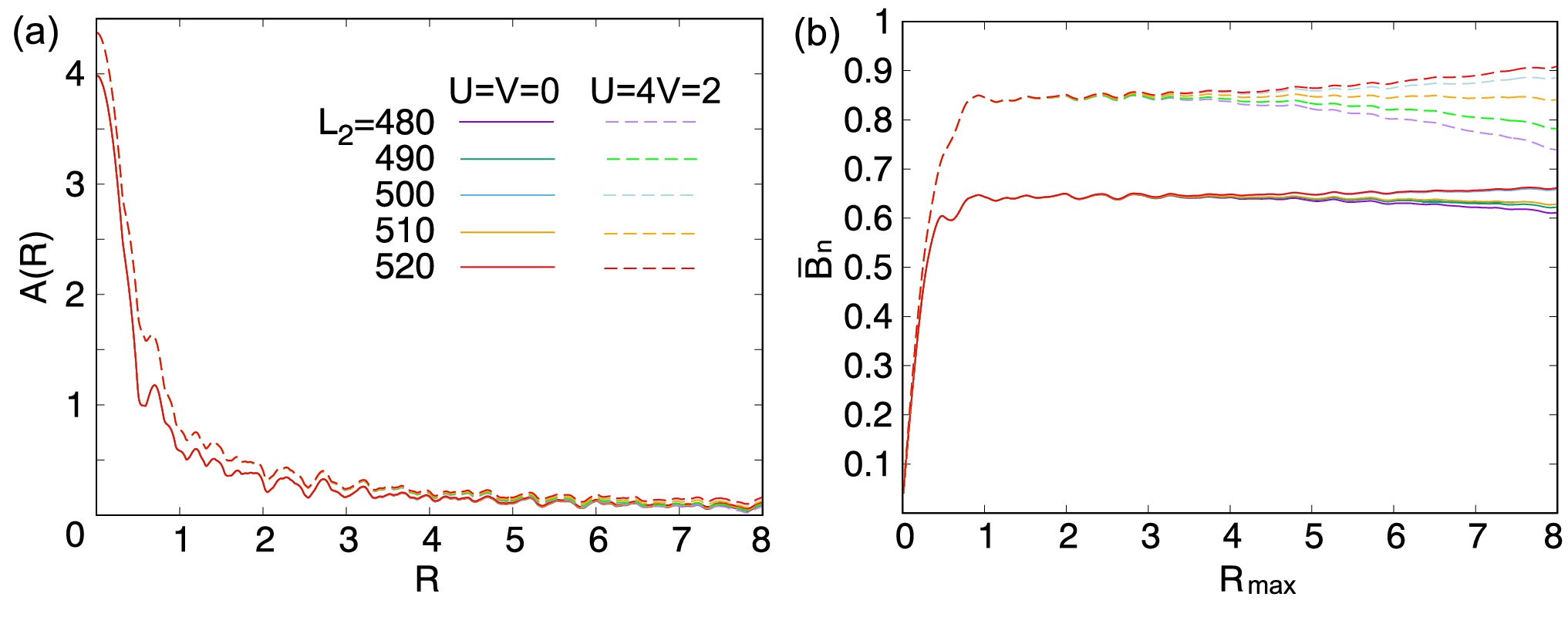
Here, we apply the idea of the hyperuniformity (Sec.II.5) Torquato and Stillinger 2003; Torquato 2016; Torquato 2018, which captures the underlying lattice structure, distinguishing it from a random distribution, and would give a measure of the regularity of the density distribution. This idea will be particularly useful when a distribution is neither characterized by symmetry breaking nor multifractality, as is the present case.

To see if a distribution is hyperuniform or not, we examine whether $A(R)$ [Eq. (14)] disappears at a large $R$. When it disappears, the hyperuniformity order metric $\bar{B}$ [Eq. (15)] gives a measure of the regularity. As is clear from Eqs. (14) and (15), these quantities reflect a nonlocal feature of the distribution beyond the local fluctuation taken into account by Eq. (17).

Figure 13 shows the $R$ ($R_{\mathrm{max}}$) dependence of $A(R)$ ($\bar{B}$) for $U=V=0$ and $U=4V=2$ at $\bar{n}=1.3$. Here, we have performed the Hartree-Fock calculation for a 1 364 431-site cluster and used a region inside a circle of the radius $L_{2}$ ($480\leq L_{2}\leq 520$) around the center for calculating $A(R)$ and $\bar{B}$. For $\bar{B}$, we have plotted a normalized quantity, $\bar{B}_{\mathrm{n}}\equiv\bar{B}/(\phi^{1/2}\bar{n}^{2})$ with $\phi\equiv\frac{\pi N}{4v}$²² 2 This $\phi$ factor is introduced to make the definition consistent with Ref. Torquato 2016, where the order metrics of various lattices are compared to eliminate the trivial factor scaling with $\bar{n}^{2}$.

The decrease of $A(R)$ to zero with increasing $R$ shows that the density distribution is hyperuniform for both $U=V=0$ and $U=4V=2$. $\bar{B}_{\mathrm{n}}$ is nearly flat with a small fluctuation for $1\lesssim R_{\mathrm{max}}\lesssim 5$. However, for $R_{\mathrm{max}}\gtrsim 5$, $\bar{B}_{\mathrm{n}}$ shows an upward or downward shift depending on $L_{2}$, and this shift becomes large as $R_{\mathrm{max}}$ increases. This will be attributed to the finite system size.

We therefore take $R_{\mathrm{max}}=5$ to evaluate $\bar{B}_{\mathrm{n}}$, where we take the average over 50 samples of $L_{2}$ ($=471,472,...,520$ for $N=1364431$ and $=271,472,...,320$ for $N=520851$) and evaluate the error bar. The results are presented in Fig. 14 for $\bar{n}=1.3$. We see that the two averages of different ranges of $L_{2}$ give almost the same result except that the error bar is smaller for the larger $L_{2}$ range. Note that the order metric of the point set (i.e., $n_{i}\equiv 1$) is about $\bar{B}_{\mathrm{n}p}\equiv 0.60052$ Zachary and Torquato 2009; Torquato 2018, which is well reproduced by the present calculation and shown by the horizontal line.

For $U=V=0$ [see Fig. 14(a)], $\bar{B}_{\mathrm{n}}$ is about 0.644, which is substantially larger than $\bar{B}_{\mathrm{n}p}$ due to the modulation induced by $t$. As $U$ increases, $\bar{B}_{\mathrm{n}}$ decreases monotonically in accord with the intuition that the density fluctuation is suppressed: It will approach $\bar{B}_{\mathrm{n}p}$ in the large $U$ limit. When $V$ is introduced with $U=2$ fixed [Fig. 14(b)], $\bar{B}_{\mathrm{n}}$ increases significantly. Thus, the $V$-induced distribution pattern seen in Fig. 4(d) is characterized by the order metric much larger than that of the $t$-induced patterns at $V=0$ [Fig. 4(c)].

In Fig. 15, we explore the interaction effects on the hyperuniformity for various electron fillings. For $\bar{n}\leq 0.7$, $\bar{B}_{\mathrm{n}}$ does not change much with $t$, $U$, and $V$: The change is mostly within the error bar. For $\bar{n}\geq 0.9$, we see that $t$ substantially enhances $\bar{B}_{\mathrm{n}}$ while $U$ suppresses it. The effect of $V$ is nonmonotonic for $\bar{n}=0.9$ while a pronounced and monotonic increase of $\bar{B}_{\mathrm{n}}$ is seen for $\bar{n}\geq 1$. Interestingly, as a function of $\bar{n}$, $\bar{B}_{\mathrm{n}}$ takes a maximum around $\bar{n}=1$ for a large $V$. This will be because $n_{i}$ can fluctuate most strongly around $\bar{n}=1$ in the present mean-field approach. These behaviors are consistent with the results obtained in the previous sections, as well as with our intuition, demonstrating that the hyperuniformity order metric is a reasonable measure to quantify the inhomogeneous density distributions in quasiperiodic systems.